Application Analysis of the Curved Elements to a Two ... · Two-Dimensional Laplace Problem Using...

Application Analysis of the Curved Elements to a Two-Dimensional Laplace Problem Using the Boundary

Element Method

* Corresponding author. Tel.: +256772353598; email: [email protected] Manuscript submitted January 25, 2015; accepted June 4, 2015. doi: 10.17706/ijapm.2015.5.3.167-176

Abstract: The boundary element method (BEM) has had an advantage of discretizing the boundary over the

finite element method and the finite difference method for so long. The curved and straight elements are

crucial for the discretization process. In this study, the BEM has been of fundamental importance in as far as

solving a two –dimensional Laplace problem is concerned.

The BEM, finite element method (FEM), and the finite difference method (FDM) and their applications

were reviewed, with the BEM taking advantage of the other two in relation to curved and straight elements.

The Laplace equation with its boundary integral formulation was done and the BEM applied. The

Dirac-Delta and the Green’s functions were behind the use of the BEM. Finally, three model problems were

tested for analysis of the BEM and curved elements in relation to solving the Laplace problem. The MATLAB

programs and subprograms were used among others to solve the Laplace’s equation in the exterior of the

Ellipse, interior of a unit circle, calculating the element data for a Dirichlet type problem. The same

programs were used in computing the capacitance between the concentric cylinders and eventually in the

analysis.

Findings showed the fundamental advantageous stage of the curved to straight elements, the suitability

of the former to the latter when finding the potential and capacitance uniquely using the BEM. However the

method is not applicable to partial differential equations (PDEs) whose fundamental solutions cannot be

expressed in the explicit form.

Key words: Boundary, curved, capacitance, potential.

1. Introduction

There are several mathematical problems that arise in our day-to-day lives. For instance, the boundary

problems are a common phenomenon in mathematics [1]. An example of the boundary value problem is:

Let E be an open domain in RN with boundary S,

2

( ) 0, ,u x x E ( ) ( )u x g x on S (1)

where g(x) is the Dirichlet data. Such a problem can be solved by several analytical and numerical methods

which include the BEM, FEM, and FDM. The FEM and FDM are approximate and therefore their accuracy can

be improved by refining the mesh or by using elements whose shapes fit more closely to the boundary [1],

International Journal of Applied Physics and Mathematics

167 Volume 5, Number 3, July 2015

Twaibu Semwogerere*

College of Engineering Design, Art and Technology, Makerere University, P. O. Box 7062, Kampala, Uganda.

[2]. Noted however, is that the FEM with their variation principle are powerful as far as obtaining numerical

solutions to the linear or non-linear partial differential equations (PDEs) [3]. The FEM is vital in the

understanding and the use of the BEM [4]. It should be noted that the BEM is more recent than the other

two and has several advantages over the others that include among others: Discretizing at infinity [5], [6],

and its application to solving acoustic and general engineering science problems.

The manuscript mainly entailed the use of the BEM on the curved elements. This requires preliminary

studies of the Dirac-delta distributions, the Green’s functions, and the divergence theorem. Similarly, the

Laplace equation and the BEM were briefly reviewed.

1.1. The Laplace Equation

Apart from using this equation in electro-statistics, it is also used in incompressible fluid flow and for the

heat conduction in the steady state [7]. For a Laplace equation, the solutions within a given region say 𝑅,

can be found given the specification of the potential or field around the boundary. Solutions of Laplace’s

equation are called harmonic functions [8]. The Laplace’s boundary integral form required us to transform

the PDE only unlike the FEM. A function u was considered to be satisfying equation (1) to give the following

integral formulations:

2 2 2[ ( ; ) ( ( )) ( ) ( ; )] [ ( ) ( ; )]

D DG x u x S u x G x dA u x G x dA (2)

( ),

( ; ) ( ) ( ) ( ) 0.5 ( ),

0,S

u x Du G

G s x s u s s ds u x Sn n

E

(3)

where G is the Green’s function, D is the interior domain, S is the boundary and E is the exterior region.

Equation (3) is simplified from equation (2) by applying Green’s function properties, and by cosmetic

changes. This accomplishes the first stage of the BEM [1].

1.2. The Boundary Element Method (BEM)

1.2.1. Introduction

The BEM as applied to the Laplace’s equation is the most recent than the finite element and finite

difference methods [2] and [3]. In the last three decades, the method has been developed into a robust

technique for especially modeling elasticity and acoustics [8] and [9]. The term “element” meant the

geometry and type of approximation to a given variable. The term “node” was used to define the

elementgeometry or the variables involved in the problem.

In using the BEM on the interior Laplace problem, two relevant things were noted about elements;

A different number of nodes were used for the variable approximations. For instance the constant and

linear elements used the same number of nodes whereas the Gauss-Legendre elements use twice that

number [1], [2].

Since the element is made up of the geometry and type of approximation, this approximation may be

linear, quadratic or otherwise. But some of these approximations like the linear and quadratic use global

basis functions which are continuous over the boundary. Other approximations give a jump discontinuity

which may not affect the accuracy of method because of integration. Hence such discontinuities in the

basis function are acceptable for the method [2].

However, a difficulty may arise because of the normal between adjacent elements not being continuous.



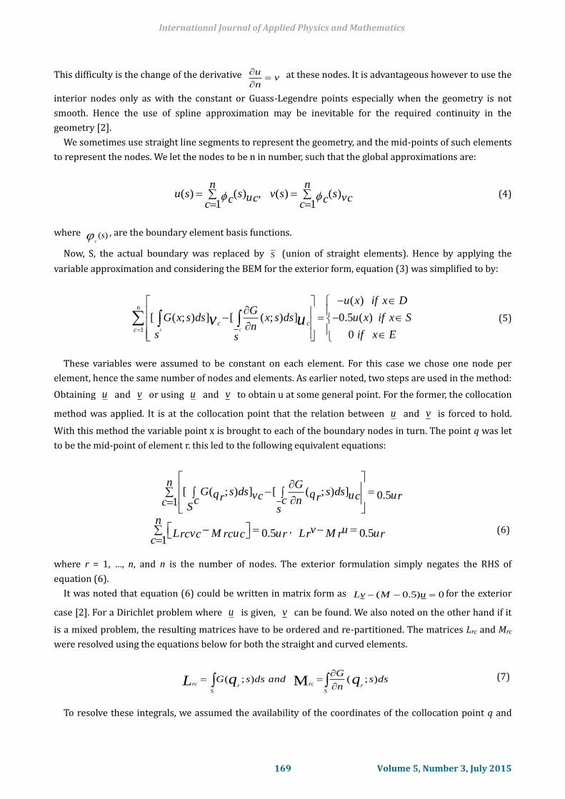
This difficulty is the change of the derivative vn

u

at these nodes. It is advantageous however to use the

interior nodes only as with the constant or Guass-Legendre points especially when the geometry is not

smooth. Hence the use of spline approximation may be inevitable for the required continuity in the

geometry [2].

We sometimes use straight line segments to represent the geometry, and the mid-points of such elements

to represent the nodes. We let the nodes to be n in number, such that the global approximations are:

( ) ( ) ,1

nu s s uccc

( ) ( )1

nv s s vccc

(4)

where )(s

c , are the boundary element basis functions.

Now, S, the actual boundary was replaced by S (union of straight elements). Hence by applying the

variable approximation and considering the BEM for the exterior form, equation (3) was simplified to by:

1

( )

[ ( ; ) ] [ ( ; ) ] 0.5 ( )

0c c

n

c cc

u x if x DG

G x s ds x s ds u x if x Sn

s if x Es

v u

(5)

These variables were assumed to be constant on each element. For this case we chose one node per

element, hence the same number of nodes and elements. As earlier noted, two steps are used in the method:

Obtaining u and v or using u and v to obtain u at some general point. For the former, the collocation

method was applied. It is at the collocation point that the relation between u and v is forced to hold.

With this method the variable point x is brought to each of the boundary nodes in turn. The point q was let

to be the mid-point of element r. this led to the following equivalent equations:

[ ( ; ) ] [ ( ; ) ] 0.51

n GG s ds s dsq qv u uc c rr rc c nc S s

0.51

nv u uL Mrc rcc c r

c

, 0.5v u uL Mr r r (6)

where r = 1, …, n, and n is the number of nodes. The exterior formulation simply negates the RHS of

equation (6).

It was noted that equation (6) could be written in matrix form as 0)5.0( uMvL for the exterior

case [2]. For a Dirichlet problem where u is given, v can be found. We also noted on the other hand if it

is a mixed problem, the resulting matrices have to be ordered and re-partitioned. The matrices Lrc and Mrc

were resolved using the equations below for both the straight and curved elements.

dssn

GanddssG qqL r

SSrrc

);( );( Mrc

(7)

To resolve these integrals, we assumed the availability of the coordinates of the collocation point q and



the end points a, b. The diagonal entries arise when q oincides with the element node. This accomplished

the first step, because at this stage v could be calculated for a Dirichlet problem [2]. In the second step u

at a general point could be found by

vxLuxMxu )()()( (8)

Resolving the matrix and integral forms for the curved elements can be found in the findings of this

manuscript.

2. Methodology

This study involved a review of the BEM, and a simple comparison of the BEM with the FEM. The

Dirac-Delta and the Green’s functions were also briefly reviewed in relation to the Laplace problem in the

finite space. The Laplace equation with its boundary integral formulation was done and the BEM applied.

The algebra behind the straight and curved elements was analyzed with more emphasis put on the curved

elements. Finally, three model problems were tested for analysis of the BEM and curved elements in relation

to solving the Laplace problem. Several MATLAB programs were used in the analysis section. They included

among others:

Beexcp.m: This uses the BEM for solving the Laplace’s equation in the exterior of the Ellipse for a

Dirichlet type problem. The same program was used in computing the capacitance between the

concentric cylinders. The element data for this program and Beextcp.m is generated by a file eltsp.m

which requires only the number of nodes and ordinates. The values of the problem variable at the

element mid-points i.e. the u data, is calculated from the exact solution. This in turn is calculated in a

function sub-program ansep.m (this returns the analytic value of a function at a sequence of points

1 1( , ),..., ( , )

n ny yx x ).

Beextc.m: It uses the BEM for solving the Laplace’s equation in the exterior of the unit circle for a

Dirichlet type problem (Beextcp5.m on the other hand uses a circle of radius 0.4). The element data, is

calculated from the exact solution. This is calculated in a function sub-program anse1.m. The function

Eltsp5.m discretizes the boundary of the circle of radius 0.4 and stores such coordinates.

Beintc.m: This uses the BEM for solving the Laplace’s equation in the interior of the unit circle as applied

to curved elements for a Dirichlet type problem. The element data (discretization), is done by the file

Elts.m while the u data is calculated from the exact solution by using the sub-program Mant2.m. This

function Mant2.m computes vectors Lr, Mr which are the rows of the boundary element matrices 𝐿 and

𝑀. The Lx, Mx ectors in the second stage of the BEM also use this function. It also uses a function called

Trapez.m to solve quadratic-in-sine integrals.

3. Findings

3.1. Computationof the Matrix Terms for Curved Elements

Some element-discretization procedures and variable approximation techniques like those above

remained the same as for the straight elements. We therefore began the computation of the terms for the

matrices Lrc and Mrc already considered in the previous section. A curved boundary element, as an arc of a

circle, AB was considered. Thus Fig. 1 illustrates the setting for computing matrix terms for the curved

element (see Fig. 1 below).

From Fig. 1, the following expressions were resolved:



aaa21

, , bbb21

, , )(5.0 abd , )1()2(2arctan dd ddms .,arcsin

mse

e

A 2

2c

, ccc

n sincos nbae

cq )cos1()(5.0 (9)

Fig. 1. The setting for computing the matrix terms for curved element.

The integrals M and L were evaluated by mapping the curved element on to [-1, 1] as seen in Fig. 2 below:

Fig. 2. Introducing t∈[-1, 1].

In Fig. 2, t is introduced to the interval [-1, 1] that bounds the element under consideration. Similarly, we

note that:

),e

t

,2 2 c

2 sin( )

2p , ,sin,cos pp ( )

cq t pq

(10)

Assuming the availability of the end points a and b and the coordinates of the collocation point qr, the

computation of the matrix terms could be done [1]. We first of all made the following simplifications;

. ( ).r n c p n

and ) )22

( ) cos( )sin2 2

e et t

r (11)

where [2 [cos ,sin ]][2 [cos ,sin ]] , ccc .])],sin,[cos2.([2



S∈[0, 1] maps to t∈[-1, 1], and from Fig. 2, S so that ddS . Similarly, we have et so

that e

d dt , implying that e

ds dt .

Equations (7) are simplified to:

( ).11

4 ) )2( ) cos( )sin

2 2

c p ndtl ce eM rct t

, ) )21

ln ( ) cos( )1 sin8 2 2

e et tl c

Lrc

(12)

The integrals in equations (12) were elevated using the trapezoidal rule with a varying number of

ordinates. The number of ordinates is denoted no in the computer program Trapez.m. However the diagonal

elements given by the integrals Mrr and Lrr equired a different approach because a singularity cannot be

avoided. The following work simplifies the terms for the singularity [10]. For the integral Mrr the vectors r

and n are orthogonal and therefore it is zero. So when q qc r

)( ) 2 sin( ).

2

et

r t p Therefore the

integral Lrr as found to have a log type singularity and consequently needed the Gaussian quadrature

approach for the improper integrals. The integral has a vertical asymptote on [-1, 1]. In this approach we

tried to isolate the singularity so that

1ln( ) ln( ) 2 1, 2, ..., .1

4 2 4 2

etl l lc c rdt r n

2

e l cr c and (13)

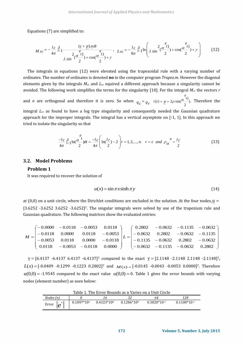
3.2. Model Problems

It was required to recover the solution of

( ) sin sinhu x x y (14)

at (0,0) on a unit circle, where the Dirichlet conditions are excluded in the solution. At the four nodes, u

[3.6252 -3.6252 3.6252 -3.6252]T. The singular integrals were solved by use of the trapezium rule and

Gaussian quadrature. The following matrices show the evaluated entries:

0000.00118.00053.00118.0

0118.00000.00118.00053.0

0053.00118.00000.00118.0

0118.00053.00118.00000.0

M

2802.00632.01135.00632.0

0632.02802.00632.01135.0

1135.00632.02802.00632.0

0632.01135.00632.02802.0

L

v [6.4137 -6.4137 6.4137 -6.4137]T compared to the exact v [2.1148 -2.1148 2.1148 -2.1148]T,

)(xL [-0.0409 -0.1299 -0.1223 0.2802]T and )(xM [-0.0145 -0.0043 -0.0053 0.0000]T. Therefore

)0,0(u -1.9545 compared to the exact value )0,0(u 0. Table 1 gives the error bounds with varying

nodes (element number) as seen below:

Table 1. The Error Bounds as n Varies on a Unit Circle

Nodes (n) 8 16 32 64 128

Error e

0.1097*101 0.4323*100 0.1286*100 0.3820*10-1 0.1100*10-1



Problem 1

We were required to find the potential outside an ellipse with radii 0.1m, 0.2m such that

2: ( ), , ( ) 10u u x x E u s and s S (15)

The wave (velocity potential) equation was used to fit this problem by assigning the sound element to

zero so as to simplify it to 2( ) 0.u x This can be reformulated by use of equation (3) so that v is the

normal component of the surface velocity and is a point on the boundary. The above procedure remains

and the potential could then be given by equation (8). The ellipse’s boundary was divided in to circular arcs

(elements), which were varied with the programs beextcp.m and eltsp.mto give the corresponding potential

in Table 2. It was assumed that u and v are constant over each element and that on

, ( ) ( ), ( ) ( ).u u and v vS j j j

Table 2. The Potential of an Ellipse

Nodes (n) 4 8 16

Potential -0.4323 -18.8639 129.1129

Finally, a problem from electro-statics required us to find the capacitance between two concentric

cylinders, the elliptic inside the circular one. The circle has radius R = 0.4m, the ellipse with radii 0.2m, and

0.1m. Two boundary conditions were given: ( ) 0 ( ) 1.u and us se c

plates. It is determined by the area/distance between the plates, and the nature of the dielectric.

We first of all did general calculations, without considering the boundary conditions. First, the ellipse was

assumed to be a sphere/circle with an average radius r1= 0.15m in order to establish the charge on the

inner plate. Similarly, the potential of the circle Vc is zero since the circle is assumed earthed. The

approximate capacitance C, is given by

41

1

RQ roCV R r

, C 26.6910pF (16)

(The permittivity of free space if the charges are in a volume, o

= 8.854 × 10-12).

Secondly, we assumed the cylinders to be a cable of some length L. We neglected any supporting disks,

and used Gauss’ law. Thus

.Q

E daSo

ln( )12

1

Q RRV E dFS rL ro

2

ln( )

1

LoC

R

r

(17)



Problem 2

Problem 3

The capacitance is the ratio of the charge on either plate Q to the potential difference, V between the

where E , is the electric field. The potential difference V is

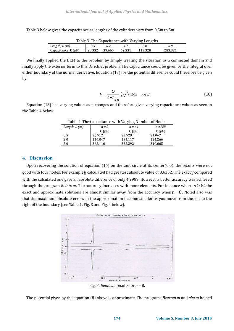
Table 3 below gives the capacitance as lengths of the cylinders vary from 0.5m to 5m.

Table 3. The Capacitance with Varying Lengths

Length, L (m) 0.5 0.7 1.1 2.0 5.0

Capacitance, C (pF) 28.332 39.665 62.331 113.328 283.321

We finally applied the BEM to the problem by simply treating the situation as a connected domain and

finally apply the exterior form to this Dirichlet problem. The capacitance could be given by the integral over

either boundary of the normal derivative. Equation (17) for the potential difference could therefore be given

by

3( )

2

QV x dx x EcV

Lo

(18)

Equation (18) has varying values as n changes and therefore gives varying capacitance values as seen in

Table 4. The Capacitance with Varying Number of Nodes

Length, L (m) n = 8 n = 64 n =128

C (pF) C (pF) C (pF) 0.5 36.512 33.529 31.067 2.0 146.047 134.117 124.266 5.0 365.116 335.292 310.665

4. Discussion

Upon recovering the solution of equation (14) on the unit circle at its center(0,0), the results were not

good with four nodes. For example u calculated had greatest absolute value of 3.6252. The exact v compared

with the calculated one gave an absolute difference of only 4.2989. However a better accuracy was achieved

through the program Beintc.m. The accuracy increases with more elements. For instance when 64n the

exact and approximate solutions are almost similar away from the accuracy when 8n . Noted also was

that the maximum absolute errors in the approximation become smaller as you move from the left to the

right of the boundary (see Table 1, Fig. 3 and Fig. 4 below).

Fig. 3. Beintc.m results for n = 8.



the Table 4 below:

The potential given by the equation (8) above is approximate. The programs Beextcp.m and elts.m helped

in the generation of the potential of this ellipse. For the condition 10)( su , the potential was seen to be

increasing as n increases as seen in Table 2 above. This was conformable with the fact that the more the

boundary of the ellipse is discretized, the better it is approximated and the better the accuracy of the

solution. The same ellipse was made to be the inner cylinder and the circle of radius 0.4, the outer cylinder.

It is hardly possible to find the capacitance if the charges on the inner and outer cylinders is different. The

BEM with curved elements can cater for this through the approximation of the boundary more closely with

increased discretization. Therefore the capacitance that follows equation (16) could be compared to that in

Table 3 for the smallest length considered. The capacitance in Table 3 was observed to be better because the

cylinder was assumed some length L. As this length increased, the capacitance was increasing as well

because it should be proportional to its length.

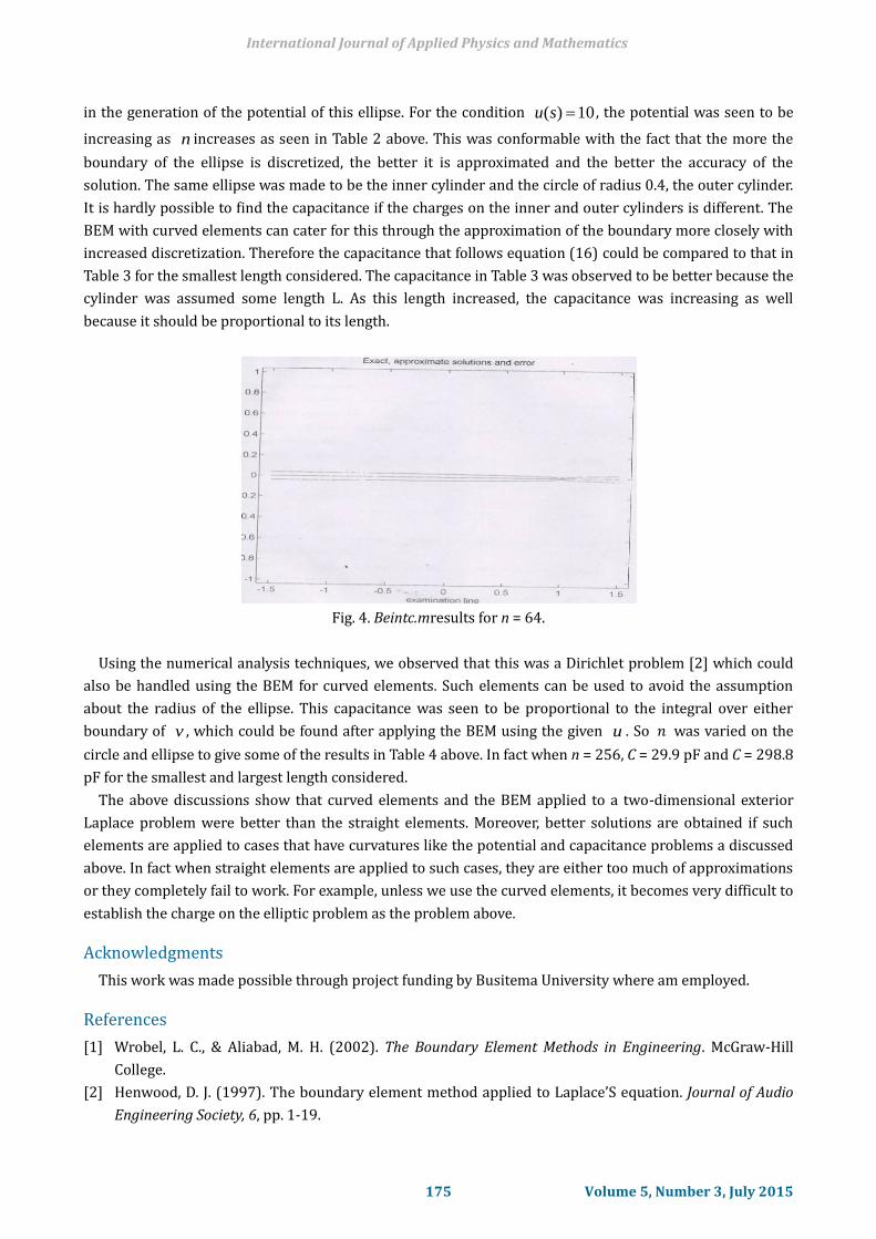
Fig. 4. Beintc.mresults for n = 64.

Using the numerical analysis techniques, we observed that this was a Dirichlet problem [2] which could

also be handled using the BEM for curved elements. Such elements can be used to avoid the assumption

about the radius of the ellipse. This capacitance was seen to be proportional to the integral over either

boundary of v , which could be found after applying the BEM using the given u . So 𝑛 was varied on the

The above discussions show that curved elements and the BEM applied to a two-dimensional exterior

Laplace problem were better than the straight elements. Moreover, better solutions are obtained if such

elements are applied to cases that have curvatures like the potential and capacitance problems a discussed

above. In fact when straight elements are applied to such cases, they are either too much of approximations

or they completely fail to work. For example, unless we use the curved elements, it becomes very difficult to

establish the charge on the elliptic problem as the problem above.

Acknowledgments

This work was made possible through project funding by Busitema University where am employed.

References



circle and ellipse to give some of the results in Table 4 above. In fact when n = 256, C = 29.9 pF and C = 298.8

pF for the smallest and largest length considered.

[1] Wrobel, L. C., & Aliabad, M. H. (2002). The Boundary Element Methods in Engineering. McGraw-Hill

College.

[2] Henwood, D. J. (1997). The boundary element method applied to Laplace’S equation. Journal of Audio

Engineering Society, 6, pp. 1-19.

[3] Chen, G., & Zhou, J. (1992). Boundary Element Method. Academic Press Ltd: Harcourt Brace Jovanovich

Publishers, London. pp. 1-16, 135-190, 374-403.

[4] Henwood, D. J., & Kirkup, S. M. (1994). An empirical analysis of the boundary element method applied

to Laplace’S equation. Journal of Applied Mathematical Modeling, 2, 32-36.

[5] Curtis, F. G., & Wheatly, O. P. (1994). Applied Numerical Analysis. Wadsworth Publishing Company, 5th ed.,

Belmont, California.

[6] Rjasanow, S., & Weggler, L. (2013). Accelerated high order BEM for maxwell problems. Journal of

Computational Mechanics, 51, 431-441.

[7] Dennemeyer, R. (1968). Introduction to Partial Differential Equations and Boundary Value Problems.

Mc-Graw-Hill, Inc. USA. pp. 92-156.

[8] Zhu, S., Satravaha, P., & Lu, X. (1994). Solving linear diffusion equations with the dual reciprocity

method in Laplace space. Journal of Engineering Analysis with Boundary Elements, 13, 309-318.

[9] Bremer, J., & Gimbutas, Z. (2012). A nystrom method for weakly singular integral operators on surfaces.

Journal of Computational Physics, 231, 4885-4903.

[10] Fata, S. N. (2009). Explicit expressions for 3D boundary integrals in potential theory. Journal of

Numerical Methods in Engineering, 78, 32-47.

Twaibu Semwogerere was born in August, 1973, and holds a bachelor of science

education degree (1995) (mathematics), master of science degree (2002) (applied

mathematics) of Makerere University, Kampala, Uganda He has a work experience of

over 21 years in colleges and university teaching. He published several papers, the

previous one being: “The erosion model for maintenance of gravel roads in Uganda:

Exploration and analysis” in the proceedings of the 9th Regional Collaboration

Conference on Advances in Engineering and Technology. He is currently a Ph. D student

(engineering mathematics) in the College of Engineering Design, Art, and Technology (CEDAT), Makerere

University and a senior lecturer at Busitema University. His areas of research and teaching include

stochastic processes, probability theory, and numerical analysis.



Application Analysis of the Curved Elements to a Two ... · Two-Dimensional Laplace Problem Using...

Documents

Transcript of Application Analysis of the Curved Elements to a Two ... · Two-Dimensional Laplace Problem Using...