Apples to Apples - RMA...Apples to Apples: A Study of Rural Municipal Finance in Alberta 5 | Alberta...
58
Apples to Apples Rural Municipal Finance in Alberta A Discussion Paper Prepared by the Alberta Association of Municipal Districts & Counties
Transcript of Apples to Apples - RMA...Apples to Apples: A Study of Rural Municipal Finance in Alberta 5 | Alberta...

Apples to Apples: A Study of Rural Municipal Finance in Alberta — Technical Appendix
1 | Alberta Association of Municipal Districts & Counties
Apples to ApplesRural Municipal Finance in Alberta
A Discussion Paper Prepared by the Alberta Association of Municipal Districts & Counties
Apples to Apples: A Study of Rural Municipal Finance in Alberta
2 | Alberta Association of Municipal Districts & Counties
Apples to ApplesRural Municipal Finance in Alberta
Written by Acton Consulting Ltd.
Published by the Alberta Association of Municipal Districts & Counties
Copyright © 2013. The Alberta Association of Municipal Districts and Counties

Don’t try to solve city problems by picking rural Alberta’s pocket
Rural Alberta is being targeted for the money it collects. As home to the robust industries that drive the province’s economy, there has been an increasing push for rural municipalities to share their perceived wealth with urban neighbours.
Why? Well, it’s true: rural municipalities do raise significant funds through taxes on those industries. Some suggest rural Alberta is unfairly wealthy when you look at how much revenue a county or municipal district collects per person.
But that’s only half the picture. Equally real are the large costs incurred to provide municipal services in rural areas that have low populations and a lot of industry. Per person, the costs are staggering.
But per person or population-based comparisons don’t work in Alberta. They can’t. One size just does not fit all.
Similarly, looking only at revenues is simplistic and, in many cases, misinformed. Is a business considered profitable based solely on how much money it makes? Of course not. It is about how much money you have left over after paying the bills. For rural Alberta, those bills carry a high price.
Preface
The bottom line is the same — we all could use more money to meet
the needs of Alberta’s people and industries.No matter where we live, we all rely on rural areas to provide the essentials of daily life: gas for heating, oil for our cars, wood for our homes, and grain and meat for food. These industries are nested in rural Alberta because it has the land and resources to support production and bring those products to market.
But that infrastructure comes with a cost. Rural municipalities manage the majority (72 per cent or 131,000 km) of Alberta’s roads and highways and 59 per cent (8,500) of all bridges. At a cost of $500,000 to $1 million for every kilometre of road and bridges coming in at anywhere from a few hundred thousand to more than a million dollars to replace, the costs are significant.
Much of this infrastructure was built in the 1950s and 1960s and is overdue for replacement. Technology and industry don’t stand still either. That aging infrastructure is not meant to carry the type, volume and weight of heavy industrial and agricultural activity that is the reality in Alberta’s robust economy.
Further, rural Alberta is a good neighbour to cities and towns. By and large, we pay for what we use through cost-sharing agreements. That way, our taxpayers know exactly where their hard-earned tax dollar is going and what benefit they get. What resident, rural or urban, would accept anything less?
Overall, rural communities simply have more roads and bridges to service than money to pay for it. Urban centres have similar challenges with providing services that rural Albertans can only dream about.
The bottom line is the same — we all could use more money to meet the needs of Alberta’s people and industries.
However, picking our back pocket is not the solution.
Bob Barss President, Alberta Association of Municipal Districts and Counties
— Originally appeared as a featured letter in the Edmonton Journal (September 5, 2013).

Apples to Apples: A Study of Rural Municipal Finance in Alberta
4 | Alberta Association of Municipal Districts & Counties
ContentsExecutive Summary .............................. 5
Introduction ........................................... 6 Preliminary Expectations .............................. 6 Methodology ................................................ 7 Definitions .................................................... 8
Trends & Reliance on Resource-Based Taxation Revenue...... 9
Importance of Linear Taxation Revenue to Rural Communities .......... 12
Should Restricted Municipal Reserves be Considered an Indication of Wealth or a Financing Tool? ............. 15 The Current Level of Reserves Held by Municipalities .................... 15 The Current Levels of Long-Term Debt Carried by Municipalities ....................... 17 A Closer Look at Reserves and Borrowing................................................. 18 The Rural Municipal Infrastructure Deficit ....................................... 19
The Extent To Which Municipalities Rely on Government Transfers For Capital Projects ................................. 25
Impact of Per Capita Funding ................ 28 A Better Predictor for Municipal Expenses ..... 33
Current Cost & Revenue Sharing Agreements ............................... 35
Summary & Conclusions ....................... 37 Summary of Findings .................................... 37 Conclusions ................................................... 38

Apples to Apples: A Study of Rural Municipal Finance in Alberta
5 | Alberta Association of Municipal Districts & Counties
Executive SummaryDiscussions on municipal finances cannot focus solely on revenues. To compare apples to apples, expenditures must be considered in assessing the differences between the urban and rural context. For rural municipalities, expenses are often higher due to their unique mix of assets, such as extensive road networks, bridges and water and wastewater systems that needs to be maintained. These assets, and the resources they help access, are a vital part of Alberta’s current economic prosperity.
In an effort to equip AAMDC members and educate other municipal stakeholders, the AAMDC, working with Acton Consulting, has commissioned this study on the current state of rural municipal finances and to determine how vital the current taxation system is to the long-term financial viability of rural municipalities.
This paper is a comprehensive analysis of municipal finances in rural Alberta. It presents 15 unique findings on the current state of both rural municipal expenses, revenues and reserves. It also examines the potential impact of reallocating linear property revenue based on population.
In going beyond simple revenue comparison, this paper seeks to provide a more objective and holistic analysis of the current state of rural municipal finances in Alberta. To accomplish this, Apples to Apples examines the following questions:
1. Are there trends in resource-based taxation revenue and to what level do rural municipalities depend on these revenue resources?
2. How important is linear taxation revenue to rural communities?
3. Should restricted municipal reserves be considered an indication of wealth or a financing tool?
4. What is the state of the municipal infrastructure deficit? How does that relate to overall municipal finance?
5. What is the validity of per capita funding arguments in the province? What impact would they have on municipalities?
6. What is the level of funding transferred inter-municipally through cost and/or revenue sharing agreements?
The answers to these questions all support the AAMDC’s position that only comparing urban and rural municipal revenues and reserves is misleading. The reality is that every municipality in Alberta faces challenges in terms of financial sustainability and continues to rely on federal and provincial grants and transfers. These challenges, however, are not identical, nor can they be solved with a one-size-fits-all solution. For while the perception is that population may be the best predictor of expenses in municipalities, in reality, assets are a far better predictor for need. These assets are critical to the support of the development of the natural resources that drive Alberta’s economy.
Apples to Apples: A Study of Rural Municipal Finance in Alberta
6 | Alberta Association of Municipal Districts & Counties
The AAMDC believes the idea that all tax revenue
from linear properties should be shared based on population is short-sighted
and not in the best interests of Albertans
– rural or urban.
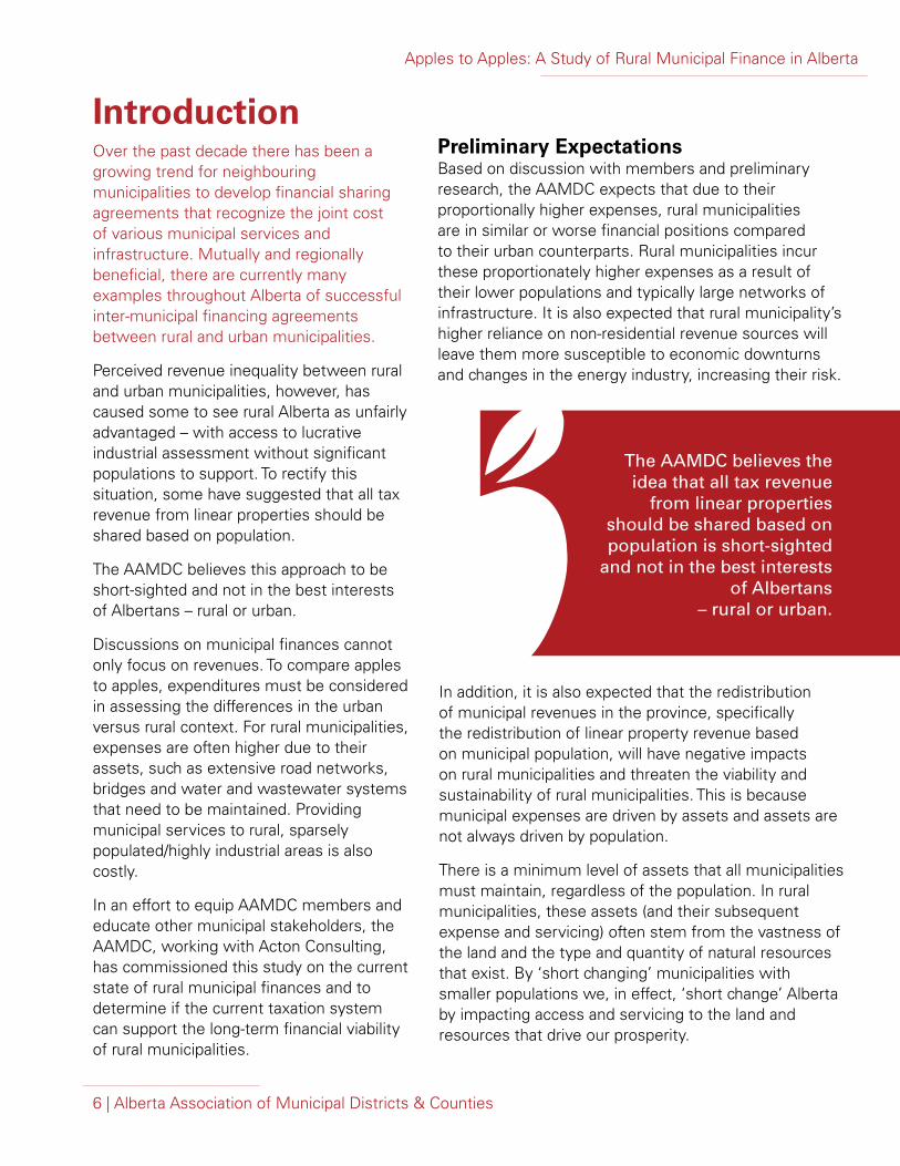
Preliminary Expectations Based on discussion with members and preliminary research, the AAMDC expects that due to their proportionally higher expenses, rural municipalities are in similar or worse financial positions compared to their urban counterparts. Rural municipalities incur these proportionately higher expenses as a result of their lower populations and typically large networks of infrastructure. It is also expected that rural municipality’s higher reliance on non-residential revenue sources will leave them more susceptible to economic downturns and changes in the energy industry, increasing their risk.
IntroductionOver the past decade there has been a growing trend for neighbouring municipalities to develop financial sharing agreements that recognize the joint cost of various municipal services and infrastructure. Mutually and regionally beneficial, there are currently many examples throughout Alberta of successful inter-municipal financing agreements between rural and urban municipalities.
Perceived revenue inequality between rural and urban municipalities, however, has caused some to see rural Alberta as unfairly advantaged – with access to lucrative industrial assessment without significant populations to support. To rectify this situation, some have suggested that all tax revenue from linear properties should be shared based on population.
The AAMDC believes this approach to be short-sighted and not in the best interests of Albertans – rural or urban.
Discussions on municipal finances cannot only focus on revenues. To compare apples to apples, expenditures must be considered in assessing the differences in the urban versus rural context. For rural municipalities, expenses are often higher due to their assets, such as extensive road networks, bridges and water and wastewater systems that need to be maintained. Providing municipal services to rural, sparsely populated/highly industrial areas is also costly.
In an effort to equip AAMDC members and educate other municipal stakeholders, the AAMDC, working with Acton Consulting, has commissioned this study on the current state of rural municipal finances and to determine if the current taxation system can support the long-term financial viability of rural municipalities.
In addition, it is also expected that the redistribution of municipal revenues in the province, specifically the redistribution of linear property revenue based on municipal population, will have negative impacts on rural municipalities and threaten the viability and sustainability of rural municipalities. This is because municipal expenses are driven by assets and assets are not always driven by population.
There is a minimum level of assets that all municipalities must maintain, regardless of the population. In rural municipalities, these assets (and their subsequent expense and servicing) often stem from the vastness of the land and the type and quantity of natural resources that exist. By ‘short changing’ municipalities with smaller populations we, in effect, ‘short change’ Alberta by impacting access and servicing to the land and resources that drive our prosperity.

Apples to Apples: A Study of Rural Municipal Finance in Alberta
7 | Alberta Association of Municipal Districts & Counties
Finding 1 Municipal Financial Information System (MFIS) reporting in Alberta needs to be improved During our analysis we encountered a number of challenges based on inconsistencies in financial reporting. This was evident in MFIS reporting, particularly after the introduction of TCA practices. It will be important to continue to provide clarity and training on municipal financial reporting to ensure consistency. This consistency will improve transparency for citizens, will make it easier to plan for municipalities, and will make it easier to plan and develop policy for the Government of Alberta.
The Core of the Matter
Methodology While not all results are outlined in this paper, the key areas investigated in this paper include: Municipal Expense Drivers, Revenue Sources, Expense Sources, Reserves and Debt and Rural Municipal Infrastructure Deficit.
To analyze these key areas a number of tools were used, including regression analysis, Municipal Financial Information System (MFIS) data, workbooks for inter-municipal transfer data capture, as well as a deterioration model.
The MFIS data was used to develop a number of ratios that provide insight into the current state of municipal finances in the province. The ratios were calculated over an eight year period, from 2004 to 2011, in order to identify any longer term trends in the ratios. MFIS data was only available up to 2011 at the time of analysis.
The workbooks were developed to capture the level of inter-municipal transfers that occur between rural and urban municipalities in the province. The level of transfers are intended to describe the cost sharing that occurs between municipalities in the province, but also capture some revenue sharing arrangements between rural and urban municipalities.
The deterioration curve used an existing model from the AAMDC’s Rural Transportation Funding Options Report (2006). The analysis shows the current state of rural municipal infrastructure in the province and was updated to the year 2011, using the most current information available. The model shows the impact of MSI funding and municipal investment in rural municipal infrastructure in the province. One of the key research topics was to analyze the infrastructure deficit and determine the impact that may have on municipal finances1.

Apples to Apples: A Study of Rural Municipal Finance in Alberta
8 | Alberta Association of Municipal Districts & Counties
Definitions There are a number of terms used in this paper that have specific definitions within the context of the report. The precise meaning of the terms within the paper is important to understand for context and consistency. These terms are consistent with other AAMDC papers, but may differ from the definitions used by other organizations.
Revenue sharing The redistribution of revenue between municipalities based on some predetermined model or formula. The particular focus for this study is revenue sharing based on allocation by population. AAMDC does not support revenue (tax) sharing among local governments as a desirable means of addressing regional financing of capital initiatives or the funding of service delivery, especially if the tax sharing is in the form of a grant from one local government to another.
Cost sharing Benefit-based cost sharing takes many forms but all involve an agreement between municipalities where those who benefit from a service pay for that service. AAMDC considers cost sharing the most effective and accountable means of cooperative financing in use by Alberta’s municipalities.
High Risk Revenue High risk revenue sources include machinery and equipment (M&E) as well as resource-related linear property revenue2. These revenues are subject to change based on fluctuations in the economy or specific markets over a relatively short period of time, making them less predictable.
Regression Analysis A statistical method measuring the strength of the predictive relationship of multiple variables. It can be used to determine the predictive power of one variable on another. Please see the Technical Appendix for more detail on regression analysis.
Operating Expenses Expenses involved in ongoing operations and maintenance of municipalities. In this report operational expenses are based on MFIS criteria and definitions.
Capital Expenses Expenses directly related to capital assets including purchasing, constructing and upgrading that extends the useful life of the asset. In this report capital expenses are based on MFIS criteria and definitions.
Tangible Capital Assets (TCA) A system of municipal financial reporting for municipalities to record and report their capital assets in their financial statements, including information on the condition of those assets. The changes to reporting involved recognizing capital expenditures, capital assets and to amortize (depreciate) them over their expected useful life. They were implemented for the 2009 reporting year. For the purpose of this paper, a number of financial ratios were impacted by changes in TCA, particularly ratios involving capital or operational expenses, as these changed in the transition. TCA also impacted the levels of reserves, as municipalities had to dedicate more of their reserves to capital projects under the new regime.
Own-Source Revenue Includes all revenue a municipality takes in from its own operations. This includes a combination of property tax revenue, fees and rentals. This does not include transfers from other orders of government. This is based on the MFIS definitions and criteria.
Outlier The most extreme examples in any set of data. For example, when discussing population urban outliers are generally Calgary and Edmonton and rural outliers include the RM of Wood Buffalo and Strathcona County.

Apples to Apples: A Study of Rural Municipal Finance in Alberta
9 | Alberta Association of Municipal Districts & Counties
Expense, not revenue, is the key driver in municipal finance.
As a rule, municipalities usually set budgets by first determining expenses and then sourcing revenue. Expenses, however, are not solely driven by population. There is a minimum level of assets that all municipalities must maintain, regardless of the population. In rural municipalities, these assets (and their subsequent expense and servicing) often stem from the vastness of the land and the type and quantity of natural resources that exist. Accessing and developing these assets is a big part of economic development (and the subsequent high quality of life) in Alberta.
Significant revenue, therefore, is required by all municipalities – regardless of population.
In our analysis, we found that rural municipalities in the province have higher risk in their revenue portfolio compared to their urban counterparts. Rural municipalities have a significantly higher reliance on volatile and risky own-source revenue sources compared to urban municipalities (i.e. reliance on the Machinery and Equipment (M&E) Tax). This revenue is considered high risk because not only just because is transitory, but also because the related revenue is dependent on a number of uncontrollable variables (e.g. amount of product running through pipelines, potential for abatement, overall industry health, world economics, etc).
High risk revenue brings uncertainty to the rural financial situation, as higher risk revenue sources are more prone to decreasing or being eliminated. This potential for volatility makes it difficult for municipal administrators to plan long-term. Without predictable and consistent revenues, it is difficult to plan capital projects, to service interest payments, and to provide consistent levels of service to citizens.
Trends & Reliance on Resource-based Taxation Revenue
Without predictable and consistent revenues, it is difficult to plan capital
projects, to service interest payments, and to provide consistent levels of
service to citizens.

Percent of Municipalities with Machinery and Equipment Tax Revenue / Total Revenue > 10%Chart 1.
Chart 1 demonstrates that more and more rural municipalities are relying on M&E taxation as a significant portion of their revenue stream. This is in contrast to urban municipalities who have held very constant. This chart intentionally understates the reliance of Albertan municipalities on high risk revenue sources by excluding the resource related linear property tax revenue and only examining M&E.
This shows the percentage of municipalities who had greater than 30% of their total revenues from linear property and M&E combined. This was done by adding linear property revenues to M&E and dividing by total revenues. This likely overstates the reliance on high risk revenue as part of the linear assessment will go towards more permanent utilities, particularly in the urban municipalities.
From this chart we see in 2004, that 76% of rural municipalities had greater than 30% of their revenue from linear property and M&E tax revenue sources; by 2011 this had increased to 82% of rural municipalities. Over the same time period the percentage of urban municipalities with greater than 30% of their revenue coming from linear and high risk sources stayed relatively flat; ranging from 0% to 3% of municipalities. The rural municipalities’ higher reliance on M&E and linear property means that their revenue streams are higher risk and more exposed to economic swings.
Percent of Municipalities with Linear Property Tax (plus M& E) / Total Revenue > 30%Chart 2.
80%
70%
60%
50%
40%
30%
20%
10%
0%2004 2005 2006 2007 2008 2009 2010 2011
Rural
Urban
70%
60%
50%
40%
30%
20%
10%
0%2004 2005 2006 2007 2008 2009 2010 2011
80%
90%
100%
Rural
Urban

Apples to Apples: A Study of Rural Municipal Finance in Alberta
11 | Alberta Association of Municipal Districts & Counties
Finding 2 Rural municipalities are increasingly reliant on higher risk revenue sourcesCharts 1 and 2 understate and overstate the reliance of municipalities on high risk revenue sources, respectively. This is a proxy for the reliance on resource based revenue. We found rural municipalities to be much more reliant on high-risk revenue and, by association, resource tax based revenue, compared to their urban counterparts.
The Core of the Matter
Apples to Apples: A Study of Rural Municipal Finance in Alberta
12 | Alberta Association of Municipal Districts & Counties
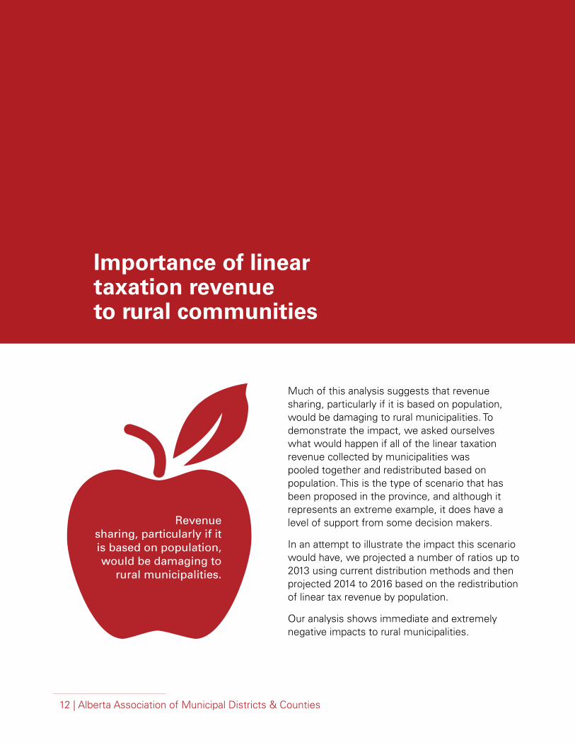
Much of this analysis suggests that revenue sharing, particularly if it is based on population, would be damaging to rural municipalities. To demonstrate the impact, we asked ourselves what would happen if all of the linear taxation revenue collected by municipalities was pooled together and redistributed based on population. This is the type of scenario that has been proposed in the province, and although it represents an extreme example, it does have a level of support from some decision makers.
In an attempt to illustrate the impact this scenario would have, we projected a number of ratios up to 2013 using current distribution methods and then projected 2014 to 2016 based on the redistribution of linear tax revenue by population.
Our analysis shows immediate and extremely negative impacts to rural municipalities.
Importance of linear taxation revenue to rural communities
Revenuesharing, particularly if it is based on population,would be damaging to
rural municipalities.

Apples to Apples: A Study of Rural Municipal Finance in Alberta
13 | Alberta Association of Municipal Districts & Counties
60%
50%
40%
30%
20%
10%
0%2013 2014 2015 2016
Rural
Urban
Urban & rural long-term debt levels in proportion to municipal debt limit, adjusted for linear taxation revenue sharing based on population
Chart 3.
Assuming municipal debt continues to grow at its current rate, this shows the minimal impact to urban municipalities, increasing their debt ratio by approximately 10% over the projection. Rural municipalities are much more significantly impacted in this projection as their debt limits decrease as a result of reduced revenues (i.e. their adjusted debt limit). We see an immediate and steep increase as soon as the reallocation model is applied in 2014. By 2016, the average rural municipality has long-term debt over 90% of its debt limit.
Forecasted percentage of municipalities in financial deficitChart 4.
Starting in 2014, we forecasted a reallocation of linear taxation revenue based on population. The chart shows an immediate effect of reallocation on rural municipalities as soon as it is applied in 2014. Roughly 50% of all rural municipalities would immediately be unable to cover their expenses. This is a drastic difference compared to 2013, before the redistribution, where there are a much smaller percentage of rural municipalities unable to cover their expenses compared to urban ones. This scenario has little impact on urban municipalities though. The number of urban municipalities unable to cover their expenses remains low (approximately 5%) and we do not see an increase after the model is applied.
70%
60%
50%
40%
30%
20%
10%
0%2013 2014 2015 2016
80%
90%
100%
Rural
Urban
Apples to Apples: A Study of Rural Municipal Finance in Alberta
14 | Alberta Association of Municipal Districts & Counties14 | Alberta Association of Municipal Districts & Counties
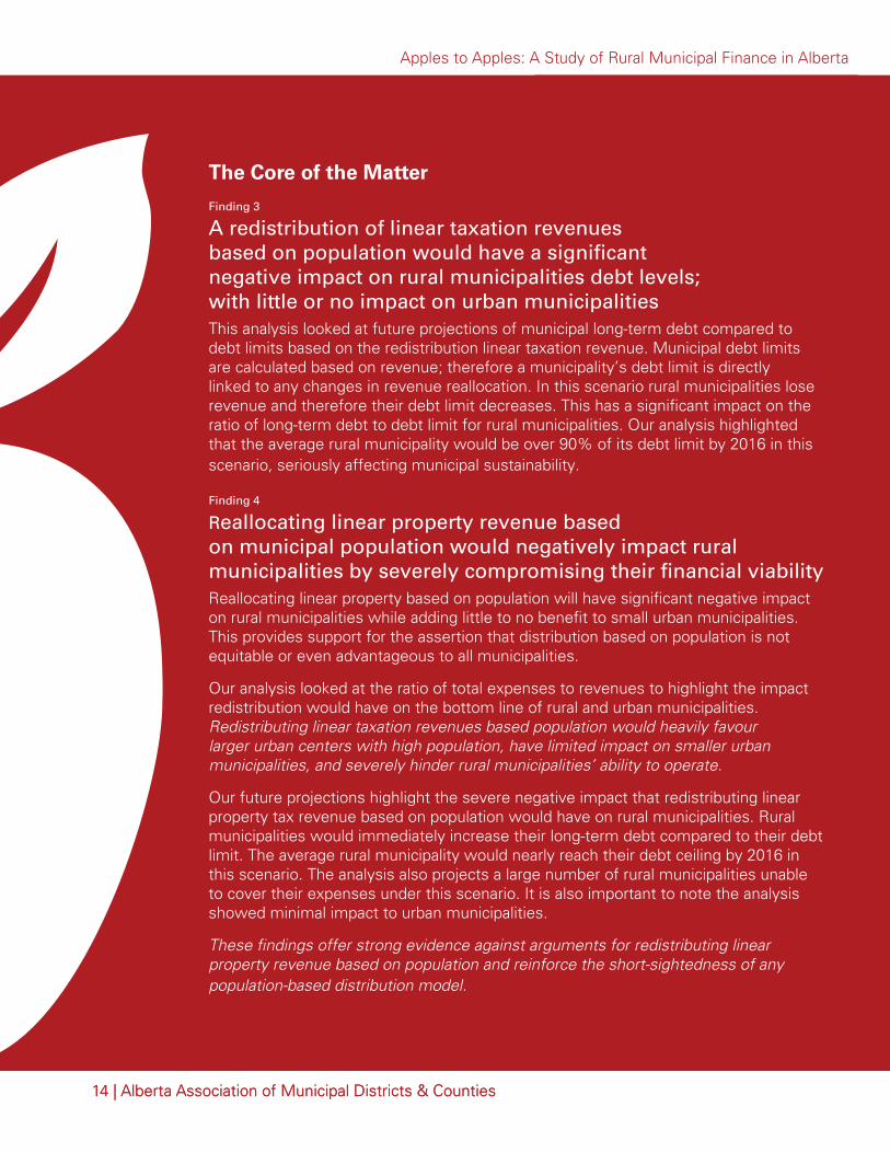
What does this mean?Finding 3 A redistribution of linear taxation revenues based on population would have a significant negative impact on rural municipalities debt levels; with little or no impact on urban municipalities This analysis looked at future projections of municipal long-term debt compared to debt limits based on the redistribution linear taxation revenue. Municipal debt limits are calculated based on revenue; therefore a municipality’s debt limit is directly linked to any changes in revenue reallocation. In this scenario rural municipalities lose revenue and therefore their debt limit decreases. This has a significant impact on the ratio of long-term debt to debt limit for rural municipalities. Our analysis highlighted that the average rural municipality would be over 90% of its debt limit by 2016 in this scenario, seriously affecting municipal sustainability.
Finding 4 Reallocating linear property revenue based on municipal population would negatively impact rural municipalities by severely compromising their financial viabilityReallocating linear property based on population will have significant negative impact on rural municipalities while adding little to no benefit to small urban municipalities. This provides support for the assertion that distribution based on population is not equitable or even advantageous to all municipalities.
Our analysis looked at the ratio of total expenses to revenues to highlight the impact redistribution would have on the bottom line of rural and urban municipalities. Redistributing linear taxation revenues based population would heavily favour larger urban centers with high population, have limited impact on smaller urban municipalities, and severely hinder rural municipalities’ ability to operate.
Our future projections highlight the severe negative impact that redistributing linear property tax revenue based on population would have on rural municipalities. Rural municipalities would immediately increase their long-term debt compared to their debt limit. The average rural municipality would nearly reach their debt ceiling by 2016 in this scenario. The analysis also projects a large number of rural municipalities unable to cover their expenses under this scenario. It is also important to note the analysis showed minimal impact to urban municipalities.
These findings offer strong evidence against arguments for redistributing linear property revenue based on population and reinforce the short-sightedness of any population-based distribution model.
The Core of the Matter
15 | Alberta Association of Municipal Districts & Counties15 | Alberta Association of Municipal Districts & Counties
Current legislation gives municipalities the autonomy to
decide how their funds are spent or saved to address infrastructure
projects. This enabling legislation is strongly supported by the AAMDC
and must be maintained.
There is a misconception that reserve levels on balance sheets are a means of measuring wealth in municipalities. Reserves are a means to pay for assets in the future. Many municipalities dedicate specific funds, called restricted reserves, to specific projects. Alternatively, some municipalities borrow to pay for these projects. Under each of these scenarios, the municipality acquires the asset, but up until completion the reserve ‘rich’ municipality appears to have greater wealth. Over the past decade, the majority of reserve funds have been dedicated to a project and are now restricted.
Restricted reserves can only be considered an indication of wealth when considered in context with all of the municipality’s assets. One must balance financial assets with the condition (and thus, value) of municipal infrastructure. Otherwise, restricted municipal reserves are simply council’s choice of financing replacement or upgrading of infrastructure.
The current level of reserves held by municipalities Municipal reserves can be restricted for a specific project (i.e. restricted reserves) or held to use for emergent issues at a later date (i.e. unrestricted reserves). The AAMDC does not have a recommended policy on holding reserves, as some municipalities choose to use them, while others do not. This decision is largely up to the political will of the constituents in each municipality.
Our analysis shows that, on average, rural municipalities have higher levels of restricted reserves than their urban counterparts. It is important to note that restricted reserves are specifically set aside for planned capital projects. Urban municipalities have typically had higher levels of unrestricted reserves. There are, however, a number of outliers that significantly increase the average reserve levels (both in urban and rural municipalities).
Given that the cost of infrastructure upgrades/replacements are typically too high to be paid out of a single year’s revenue stream, even with grant funding, councils must choose to finance the project and enjoy it now while spreading the cost over future years, or save now and put off the benefit of the new upgraded/replaced infrastructure off until years down the road.
Annual budgeted contributions to restricted reserves are considered a liability and are carried as such on municipal balance sheets. They are an indication of a council’s commitment to a future project and should not be considered part of a surplus.
Current legislation gives municipalities the autonomy to decide how their funds are spent or saved to address infrastructure projects. This enabling legislation is strongly supported by the AAMDC and must be maintained.
Should restricted municipal reserves be considered an indication of wealth or a financing tool?
Restricted reserves can only be considered an indication of wealth
when considered in context with all of the municipality’s assets.

Apples to Apples: A Study of Rural Municipal Finance in Alberta
16 | Alberta Association of Municipal Districts & Counties
Percent of municipalities with Total Reserves > One Year of Total Expenses3Chart 5.
This chart summarizes the percentage of rural and urban municipalities that had reserve levels greater than their total expenses per annum. It reveals an increasing trend in the number of municipalities that have reserve levels as high as, or higher than total expenses. In 2004, 37% of rural municipalities had total reserves greater than 100% of their annual total expenses; by 2011 this increased to 64% of municipalities. In comparison, there are fewer urban municipalities that have reserves as high as annual expenses; however the trend is also increasing. In 2004, 19% of urban municipalities had total reserves greater than 100% of their annual total expenses; by 2011 this increased to 37% of urban municipalities.
Finding 5 Both rural and urban municipalities are increasing their reserve levels Our analysis of reserves compared to total expenses shows an increasing trend in the number of rural and urban municipalities that have total reserves greater than total expenses. The ratio is total reserves divided by total expenses and represents a municipality’s ability to cover future capital projects and operational expenses in the event of decreasing revenues. As both rural and urban municipalities are increasingly reliant on revenue sources that are susceptible to unforeseen reductions (e.g. grants, transfers, resource-based revenue), it is possible that increasing reserve levels is a strategy to offset potential risk.
The Core of the Matter
60%
50%
40%
30%
20%
10%
0%2004 2005 2006 2007 2008 2009 2010 2011
Rural
Urban
70%

Apples to Apples: A Study of Rural Municipal Finance in Alberta
17 | Alberta Association of Municipal Districts & Counties
The current level of reserves held by municipalities The other typical means for financing capital projects is through borrowing. Our analysis included a review of the long-term debt levels of municipalities in the province. We compared these levels to municipal debt limits and found that this ratio had stayed relatively low for both urban and rural municipalities, which indicates debt levels are being managed appropriately.
Average municipal long-term debt compared to debt limitChart 6.
What does this mean?Finding 6 While urban and rural debt levels are relatively low in proportion to municipal debt limits, they have marginally increased over the past decadeFrom a debt perspective, rural and urban municipalities are fulfilling their financial responsibilities managing their long-term debt. The long-term debt limit is based on a formula which relies on a municipality’s revenue and ability to re-pay long-term debt. Approaching the debt limit will increase risk to the municipality and pressures its ability to service its obligations.
We found that both rural and urban municipalities are, on average, holding relatively low levels of long-term debt compared to their debt limit. However, there is a slight increasing trend for both rural and urban municipalities, and we observed that on average urban municipalities do have more long-term debt compared to their debt limit than their rural counterparts.
The Core of the Matter
Municipal debt limits are calculated as 1.5 times the current revenue of a municipality. This chart shows that, for both urban and rural municipalities, there is an increase in their ratio of long-term municipal debt to debt limit yet the majority of municipalities remain well below their overall limits. It is interesting to note that in comparison to the use of reserves, borrowing seems to have an opposite pattern with the urban municipalities using more of their debt limit than their rural counterparts. This may be an indicator of differences in financing philosophy and/or an outcome of the risk associated with rural revenue sources.
25%
20%
15%
10%
5%
0%2004 2005 2006 2007 2008 2009 2010 2011
Rural
Urban

Apples to Apples: A Study of Rural Municipal Finance in Alberta
18 | Alberta Association of Municipal Districts & Counties18 | Alberta Association of Municipal Districts & Counties
A closer look at reserves and borrowing As a part of this analysis, we indicated that typically the discussion around municipal finances in this province is centered on revenues. This is evident when we look at the arguments for redistributing linear property tax revenue. The AAMDC argues that it is critical to look at expenses, as well as revenue when discussing municipal finances. In fact, expenses are more important than revenue. A municipality’s first priority is covering their expenses in a cost efficient manner.
There are a number of “outlier” municipalities (both urban and rural) that are holding large amounts of reserves; which some would consider a measure of wealth. However, we have illustrated that the more typical rural municipalities have levels of reserves in line with the average urban municipality. There may be a few outlier rural municipalities that are driving this perception, but the reality is that a discussion of municipal wealth must include a more in-depth discussion than the currently available data will allow. Ultimately, the level of reserves must always be considered in relation to the value of a municipality’s assets.

Apples to Apples: A Study of Rural Municipal Finance in Alberta
19 | Alberta Association of Municipal Districts & Counties
Urban Reserves (Outliers Excluded)
Chart 7. Rural Reserves (Outliers Excluded)
Chart 8.
The analysis shows that on average rural municipalities have slightly higher levels of reserves overall but still proportionally similar levels of both restricted and unrestricted reserves compared to urban municipalities. Specifically rural municipalities have approximately $25 million in restricted reserves post-Tangible Capital Assets (TCA) reporting which is very similar to the average urban. The average rural does have slightly higher levels of unrestricted reserves, though not significantly. Prior to the introduction of TCA reporting4 the average rural had lower overall levels of total reserves, but higher levels of unrestricted reserves.
There is also an increasing trend in the level of restricted reserves for rural municipalities under both reporting eras (2004 to 2008 and 2009 to 2011, respectively). However our analysis also shows that unrestricted reserves were also increasing for rurals prior to TCA.
30,000,000
25,000,000
20,000,000
15,000,000
10,000,000
5,000,000
02004 2005 2006 2007
2008 2009 2010 2011
AverageUnrestrictedReserves
AverageRestrictedReserves
35,000,000
25,000,000
20,000,000
15,000,000
10,000,000
5,000,000
02004 2005 2006 2007 2008 2009 2010 2011
AverageUnrestrictedReserves
AverageRestrictedReserves
30,000,000
35,000,000

Apples to Apples: A Study of Rural Municipal Finance in Alberta
20 | Alberta Association of Municipal Districts & Counties
What does this mean?Finding 7 Rural municipal restricted reserve levels are increasing, but unrestricted reserve levels have remained flatWe looked at the current reserve levels for urban and rural municipalities (restricted and unrestricted). Reserves become restricted when they become allocated to fund a specific future capital expense, therefore increases in restricted reserves accounts for more in-depth municipal planning and forecasting of future expense needs, as well as a reflection of new reporting requirements under TCA. Restricted reserves can be considered responsible financial practices for future capital expenses. Our analysis shows rural and urban municipalities have similar levels of average restricted reserves, but rural municipalities have slightly higher levels of unrestricted reserves, on average.
In our analysis we discovered a number of urban and rural municipalities were having drastic impacts on the average reserve levels, making them seem excessively large. For the urban municipalities, the outliers were Calgary and Edmonton and the rural municipalities were Wood Buffalo and Strathcona County, among others. These outliers were removed from our analysis to show a more typical urban or rural municipality in the province.
The Core of the Matter

21 | Alberta Association of Municipal Districts & Counties
The Rural Municipal Infrastructure Deficit What is the impact of this borrowing or use of reserve accounts? These financing tools are used for capital projects; some to build new needed infrastructure and others, to refurbish or replace existing assets. A key question of this report is to determine the current level of infrastructure deficit in rural municipalities and how it impacts rural municipal finances.5
Rural infrastructure portfolios throughout Alberta are made up of capital assets such as roads, bridges, buildings, water and wastewater systems, whose benefits extends beyond a time span of one year (i.e. expected asset life). Over time, capital assets deteriorate (with the exception of land). Therefore, the value of the infrastructure portfolio naturally goes down. This can be prevented through investment in the maintenance or replacement of assets; this investment maintains and/or increases the condition (i.e. the percentage of new condition) of these assets depending on the level of investment. The infrastructure deficit is the difference between the current condition of rural municipal infrastructure and the optimal level of assets6.
The deterioration curve model was first applied to analyze the state of rural infrastructure in a 2006 AAMDC report, Rural Transportation Funding Options Report. This analysis was a key item of evidence in the design of the Municipal Sustainability Initiative in 2007. It is a mathematical formula that forecasts the condition of the overall portfolio based on the weighted average point in the assets life; in a graph format it looks like a curve.
Our analysis looked at the rural infrastructure deficit under scenarios where there was no MSI funding provided, the planned MSI funding amounts were provided, and the current reality.
The infrastructure deficit is the
difference between the current condition
of rural municipal infrastructure and the
optimal level of assets

Apples to Apples: A Study of Rural Municipal Finance in Alberta
80%
60%
40%
20%
0%
100%
20% 40% 60% 80% 100%0%
% of Expected Life Consumed
% o
f N
ew C
on
dit
ion
Asset Deterioration CurveChart 9.
This chart shows that assets do not deteriorate on a straight line basis; in their first years of service, little deterioration of their value occurs. But if the asset is left to deteriorate, the pace of deterioration continues at an increasing rate. At approximately 70% of the expected life, we see a “cliff” where deterioration accelerates very quickly. At this point it becomes extremely expensive year over year to maintain the asset. Instead it is a much better strategy to maintain the asset at the top of the curve, approximately 94% of new condition and 50% of useful life, where it takes a much smaller investment to maintain the asset year over year.
This curve shows the potential impact to municipalities if infrastructure is left to deteriorate. Municipalities run a risk of having their infrastructure reach the steep part of the curve, where repairing it becomes extremely expensive. This would put incredible pressure on municipalities to reallocate revenues from other areas to address their infrastructure issues.
Individual details on the condition and age of these assets are difficult to gather, but there are techniques to study them as a whole portfolio. For this study we looked at the previous work that had made estimates of the state of Alberta’s rural municipal infrastructure in 20067 and 20088. We then updated the model using current information up to 2011 to see the changes that have occurred since the last variation.
Using updated information, we looked at the levels of investment that have been made by rural municipalities into the rural infrastructure portfolio, and mapped them against the expected year over year deterioration of the portfolio based on the curve above. We wanted to see if the investment was outpacing the deterioration of the portfolio or vice versa. We also analyzed the addition of Municipal Sustainability Initiative (MSI) funding on the portfolio. The MSI funding was a major initiative by the provincial government to reduce the infrastructure deficit in the province.
This study also recognizes that municipalities also contribute to infrastructure from their own reserves and other federal and provincial grants and transfers9. These grants and transfer programs continue to be vital to the sustainability of rural municipal infrastructure creation and maintenance.

Apples to Apples: A Study of Rural Municipal Finance in Alberta
23 | Alberta Association of Municipal Districts & Counties
Year Actual MSI Amounts Original MSI Amounts
2007 $143,069,526 $142,929,826
2008 $169,393,843 $160,830,963
2009 $136,277,743 $195,818,640
2010 $300,856,693 $470,925,530
2011 $219,261,581 $339,332,521
Comparison of Actual vs. Original MSI Rural ContributionsChart 10.
Rural Municipal Infrastructure Deficit (Millions) Chart 11.
Here we see the annual infrastructure deficit for each of the three scenarios (Actual, Original and Without MSI) and the funding required to get the infrastructure portfolio to the optimal level. The differences between the three scenarios demonstrate the differences in annual municipal capital investment as a result of the Municipal Sustainability Initiative. The chart also emphasizes the benefit of MSI as an investment – preventing an additional $1.5 billion in infrastructure deficit for rural municipalities.
$3,000
$2,500
$2,000
$1,500
$1,000
$500
0%2004 2005 2006 2007 2008 2009 2010 2011
With OriginalCommitment
With ActualMSI
$3,500
$4,000
$4,500
$5,000
2012
Without MSI
$ m
illio
ns
Apples to Apples: A Study of Rural Municipal Finance in Alberta
24 | Alberta Association of Municipal Districts & Counties
Apples to Apples: A Study of Rural Municipal Finance in Alberta
24 | Alberta Association of Municipal Districts & Counties
Finding 8 Without the MSI program, rural Alberta’s infrastructure deficit would have been 51% higher at $4.44 billion ($4.59 billion in 2013 dollars)By 2011, the infrastructure deficit would have been $4.44 billion ($4.59 billion in 2013 dollars) if the MSI program had not been implemented. This finding demonstrates that MSI has, and will continue to work in preventing an increasing infrastructure deficit in the province.
It is also important to consider how MSI funding is being used: whether to maintain existing assets, or to build new assets. Municipalities, that are using MSI funds to build new assets, such as community centers, rather than maintaining or replacing existing assets, must be mindful of the long-term consequences. This is because building new assets will add to the size of the asset portfolio, requiring more revenue to maintain.
Finding 9 The MSI program, as it was originally designed, would have cut the rural infrastructure deficit and would have reversed the deterioration trend The original MSI funding commitment was $1.31 billion to rural municipalities over five years. This increased MSI funding would have reversed the deterioration curve and reduced the rural infrastructure deficit to $2.11 billion ($2.19 billion in 2013 dollars). This highlights that the MSI program, as it was initially envisioned, would have been an even better investment for the provincial government and would have reduced the infrastructure deficit on rural municipalities.
Finding 10 While MSI payments are slowing the increase in rural Alberta’s infrastructure deficit, the program has not eliminated the $3 billion rural infrastructure deficit Since 2007, MSI funding has helped slow the increase of the rural infrastructure deficit. By 2011, MSI had saved rural Alberta approximately $1.49 billion ($1.54 billion in 2013 dollars). While MSI has contributed to limit the deterioration of assets, it has not been enough to completely halt, let alone improve, the overall condition of rural infrastructure.
The actual MSI funding contribution to rural municipalities from 2007 to 2011 totalled $969 million and has helped limit the total infrastructure deficit to $2.94 billion ($3.05 billion in 2013 dollars).
Our analysis of the rural municipal infrastructure deficit highlights that MSI funding has been successful in limiting the deterioration of rural infrastructure in the province. However, the current levels of funding have not been enough to completely limit deterioration or improve the overall portfolio condition. This clearly shows that MSI is a critical investment in Alberta’s municipalities – preventing billions in infrastructure deficits. The significant cost saving effects of MSI also demonstrate the need for the province’s continued partnership in investing in municipal infrastructure.
The Core of the Matter

Apples to Apples: A Study of Rural Municipal Finance in Alberta
25 | Alberta Association of Municipal Districts & Counties
For both urban and rural municipalities, government transfers and grants to fund capital expenditures are essential. As responsibilities and expectations for municipal government increase, these grants and transfers will only become more vital. Without consistent and predictable funding, municipalities are hampered in their ability to create long-term plans.
The extent to which municipalities rely on government transfers for capital projects
60%
50%
40%
30%
20%
10%
0%2004 2005 2006 2007 2008 2009 2010 2011
Rural
Urban
25%
20%
15%
10%
5%
0%2004 2005 2006 2007 2008 2009 2010 2011
Rural
Urban
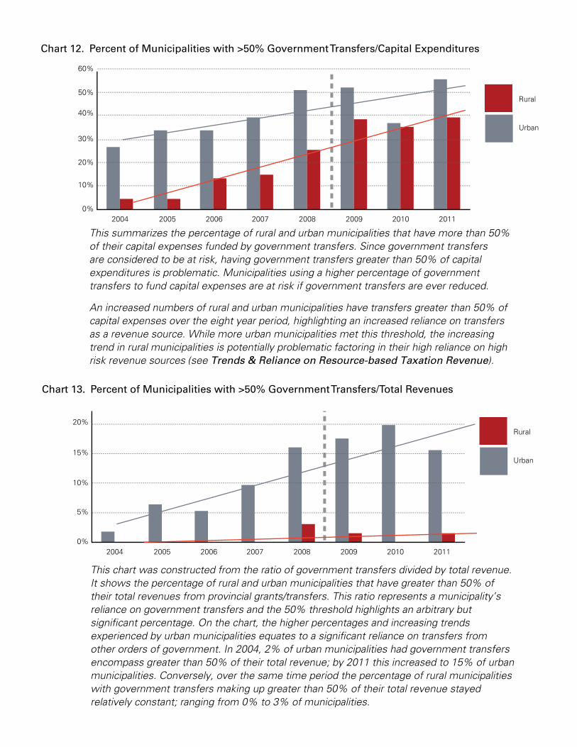
This chart was constructed from the ratio of government transfers divided by total revenue. It shows the percentage of rural and urban municipalities that have greater than 50% of their total revenues from provincial grants/transfers. This ratio represents a municipality’s reliance on government transfers and the 50% threshold highlights an arbitrary but significant percentage. On the chart, the higher percentages and increasing trends experienced by urban municipalities equates to a significant reliance on transfers from other orders of government. In 2004, 2% of urban municipalities had government transfers encompass greater than 50% of their total revenue; by 2011 this increased to 15% of urban municipalities. Conversely, over the same time period the percentage of rural municipalities with government transfers making up greater than 50% of their total revenue stayed relatively constant; ranging from 0% to 3% of municipalities.
Percent of Municipalities with >50% Government Transfers/Capital ExpendituresChart 12.
This summarizes the percentage of rural and urban municipalities that have more than 50% of their capital expenses funded by government transfers. Since government transfers are considered to be at risk, having government transfers greater than 50% of capital expenditures is problematic. Municipalities using a higher percentage of government transfers to fund capital expenses are at risk if government transfers are ever reduced.
An increased numbers of rural and urban municipalities have transfers greater than 50% of capital expenses over the eight year period, highlighting an increased reliance on transfers as a revenue source. While more urban municipalities met this threshold, the increasing trend in rural municipalities is potentially problematic factoring in their high reliance on high risk revenue sources (see Trends & Reliance on Resource-based Taxation Revenue).
Percent of Municipalities with >50% Government Transfers/Total RevenuesChart 13.
Apples to Apples: A Study of Rural Municipal Finance in Alberta
27 | Alberta Association of Municipal Districts & Counties
What does this mean?
Finding 11 Federal and provincial government grants and transfers are vital to the sustainability of both rural and urban municipalitiesThe analysis suggests urban municipalities rely on government transfers as a bigger proportion of their revenue and capital expenditures than their rural counterparts. However, there is an increasing trend for both rural and urban municipalities. A reliance on government transfers adds risk to their revenue projections, as they are outside of the municipality’s control. As responsibilities and expectations for municipal government increase, these grants and transfers will only become more vital.
The Core of the Matter
Apples to Apples: A Study of Rural Municipal Finance in Alberta
28 | Alberta Association of Municipal Districts & Counties
Recent years have seen a dramatic rise in the average annual expenditure of municipal
governments. Many credit this to Alberta’s overall increasing population, a shift in responsibility to
municipalities from higher orders of government, their efforts to slow or reduce the infrastructure
deficit, their residents’ demands for high standards of infrastructure and services, or a
combination of these and other factors.
As the reliance on transfers from other orders of government grows, it is important to test the assumption that population is the most fair and equitable means to allocate grant funds. Recent years have seen a dramatic rise in the average annual expenditure of municipal governments. Many credit this to Alberta’s overall increasing population, a shift in responsibility to municipalities from higher orders of government, their efforts to slow or reduce the infrastructure deficit, their residents’ demands for high standards of infrastructure and services, or a combination of these and other factors. The fall-back argument is generally that population increases puts increased pressure on municipal jurisdictions as Alberta continues to grow. Alternatively, there is also an argument that rural municipal expenses will be declining based on the steadily declining population in most rural municipalities. If this is true, then population will provide to be the main driver of municipal expenses and distribution of government support based on population will be a feasible argument.
To test whether population can accurately predict municipal expenses we used regression analysis, a statistical technique that attempts to explain the strength of the relationship between a number of variables. Regression analysis uses a form of averaging that represents the relationship of these variables. From this, we can determine how good a predictor one variable is for another (i.e. population for expenses).
To identify whether there are better predictors of municipal expenses, we also conducted a regression analysis on the relationship between municipal assets (length of roads, water and wastewater systems, total area, and number of households) and municipal expenses.
Impact of Per Capita Funding

Apples to Apples: A Study of Rural Municipal Finance in Alberta
29 | Alberta Association of Municipal Districts & Counties
3,000,000,000
2,500,000,000
2,000,000,000
1,500,000,000
1,000,000,000
500,000,000
0
3,500,000,000
200,000 400,000 600,000 800,000 1,000,000 1,200,000
R2 = 0.9608
To
tal E
xpen
dit
ure
s
Population
Relationship between Alberta Municipal Population and Total Expenditures – All Municipalities 2004 – 2011
Chart 14.
This chart shows the relationship between population and expenses for all Alberta municipalities over an eight year time period. Does population predict expenses? Initially, the method seems to answer this question, suggesting that 96% of the change in expenses can be predicted by change in population. However, one can see in the circled portion of the chart that the high population data points, Edmonton and Calgary, have a significant impact on the analysis.
Apples to Apples: A Study of Rural Municipal Finance in Alberta
30 | Alberta Association of Municipal Districts & Counties
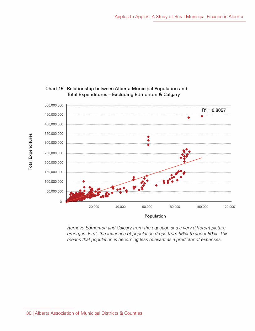
Relationship between Alberta Municipal Population and Total Expenditures – Excluding Edmonton & Calgary
Chart 15.
300,000,000
250,000,000
200,000,000
150,000,000
100,000,000
50,000,000
0
350,000,000
20,000 40,000 60,000 80,000 100,000 120,000
R2 = 0.8057
To
tal E
xpen
dit
ure
s
Population
400,000,000
450,000,000
500,000,000
Remove Edmonton and Calgary from the equation and a very different picture emerges. First, the influence of population drops from 96% to about 80%. This means that population is becoming less relevant as a predictor of expenses.
Apples to Apples: A Study of Rural Municipal Finance in Alberta
31 | Alberta Association of Municipal Districts & Counties
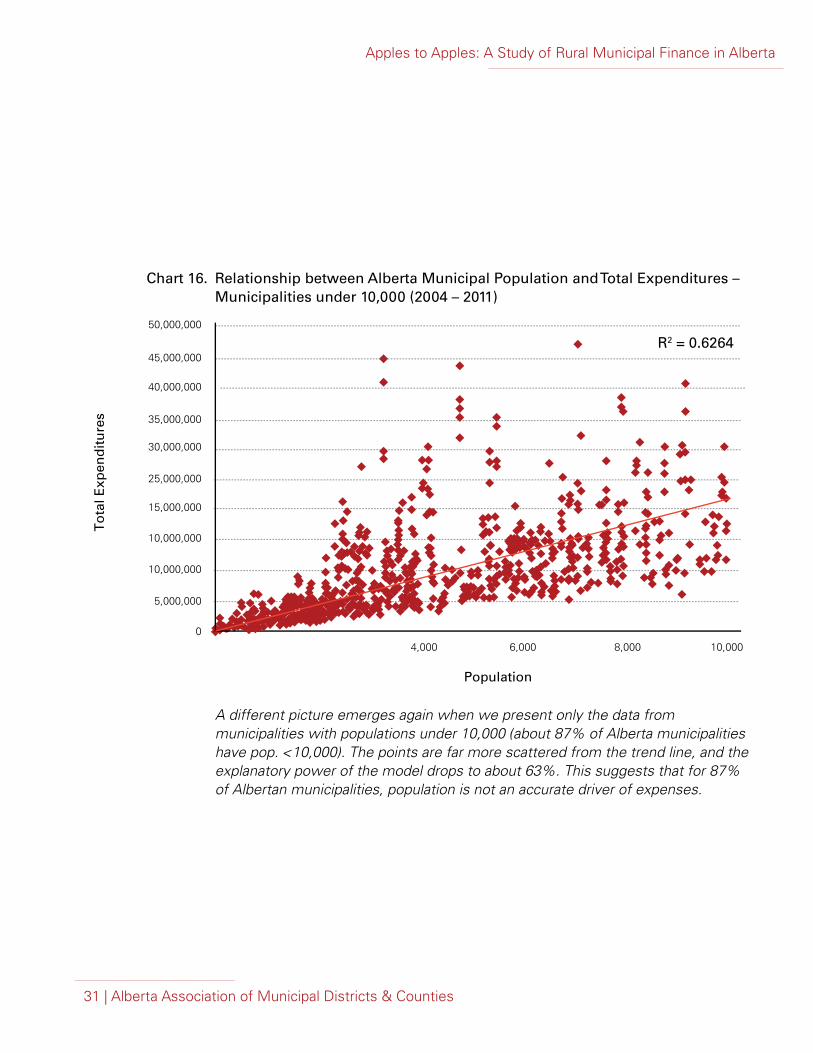
Relationship between Alberta Municipal Population and Total Expenditures – Municipalities under 10,000 (2004 – 2011)
Chart 16.
30,000,000
25,000,000
15,000,000
10,000,000
10,000,000
5,000,000
0
35,000,000
4,000 6,000 8,000 10,000
R2 = 0.6264
To
tal E
xpen
dit
ure
s
Population
40,000,000
45,000,000
50,000,000
A different picture emerges again when we present only the data from municipalities with populations under 10,000 (about 87% of Alberta municipalities have pop. <10,000). The points are far more scattered from the trend line, and the explanatory power of the model drops to about 63%. This suggests that for 87% of Albertan municipalities, population is not an accurate driver of expenses.

Apples to Apples: A Study of Rural Municipal Finance in Alberta
32 | Alberta Association of Municipal Districts & Counties
What does this mean?
Finding 12 Analysis of municipal data is misrepresented with the inclusion of Edmonton and Calgary There are fundamental differences in population, infrastructure, scope and influence of Edmonton and Calgary compared to other municipalities in the province. They should not be considered in the same analysis as other municipalities. This conclusion was highlighted in our regression analysis as Edmonton and Calgary are obvious outliers in the sample (see Chart 14). They also impacted the results of the analysis as the linkage between population and municipal expenses decreases significantly when they are removed from the analysis (see Chart 15 and 16).
The Core of the Matter
Apples to Apples: A Study of Rural Municipal Finance in Alberta
33 | Alberta Association of Municipal Districts & Counties
A Better Predictor for Municipal Expenses Total municipal population is not a good predictor of municipal expenses, particularly for smaller municipalities. Would an asset-based model work better for predicting expenses?
To test this we applied a similar methodology to municipal assets, regressing a bundle of assets (length of roads, water and wastewater systems, total area, and number of households) against municipal expenses. We ran the same analysis as our population analysis: for all municipalities, municipalities under 100,000 populations and municipalities under 10,000 populations.
Size Population Assets # of Municipalities
All 96.0% 95.0% 342
Under 100,000 80.5% 79.0% 339
Under 10,000 62.6% 83.0% 298
Population versus Asset as a Predictor of Municipal ExpensesChart 17.
The amount of assets a municipality has can predict 95% of its expenses. As an example, each additional kilometre of road and the amount of land that a municipality has will lead to higher expenses.
Four of the asset groups had a positive correlation with municipal expense as in, the greater the length of roads, water and wastewater systems, and total area of the municipality the greater cost the municipality faces. The fifth asset group (housing density) showed a negative correlation to municipal expense. In other words, the more condensed a municipality is, the lower the costs to service the municipality.10
Apples to Apples: A Study of Rural Municipal Finance in Alberta
34 | Alberta Association of Municipal Districts & Counties
What does this mean?
Finding 13 Total municipal population is not a strong driver for predicting municipal expensesFor the strong majority of municipalities in the province, their expenses are more closely related to their asset base than their population. Plans to redistribute grant funding or taxation revenue based on population therefore are likely to hurt smaller urban and rural municipalities, while helping only a small number of larger urban centers. The reality is that even in instances of declining population in rural areas, fixed costs related to infrastructure do not decline with population and need to be considered in funding models.
Finding 14 Assets are a better driver than population for predicting Alberta municipal expensesBoth analyses, for under 100,000 population and under 10,000 population, provide strong evidence that asset based models are better predictors of municipal expenses, predicting 79% and 83%, respectively. The asset based regression model does not decrease nearly as much as the population analysis when looking at smaller population groups.
This analysis also lends support to rural municipalities retaining linear tax property revenue, because the industries that supply it require a substantial infrastructure base and road network. Typically the argument is that some of the revenue should be redistributed to urban municipalities, where the workers for the industry typically live. However, our analysis shows that the asset based to support the industry is a better predictor of expenses than the population used to staff those industries.
This analysis answers the question whether population is the best driver for municipal expenses, and whether population based grant funding is appropriate. What we found is that municipal expenses are driven more by their assets compared to their population, especially in smaller municipalities. This calls into question the use of population-based allocation models for grant programs if the goal is to fund needs (i.e. expenses) in the fairest manner.
The Core of the Matter

Apples to Apples: A Study of Rural Municipal Finance in Alberta
35 | Alberta Association of Municipal Districts & Counties
100
80
60
40
20v
02004 2005 2006 2007 2008 2009 2010 2011
120
140
2011
$ m
illio
ns
Increasingly inter-municipal transfers represent cost sharing initiatives between rural and urban municipalities.11 Typically, and inappropriately, these inter-municipal transfers are often ignored in discussions of municipal finances in the province.
Current Cost & Revenue
Sharing Agreements
Rural to Urban Inter-municipal Transfers Chart 18.
Since 2004, anywhere from $45 million to $130 million has been transferred from rural to urban municipalities. In general, an increase in transfers is seen year over year. However, there is evidence to suggest that this significant drop is due to the lack of complete data in 2011 and 2012 as well as the potential delays in the completion of capital projects in urban centers, which received contributions from rural municipalities.

Apples to Apples: A Study of Rural Municipal Finance in Alberta
36 | Alberta Association of Municipal Districts & Counties
What does this mean?
Finding 15 Rural municipalities make substantial contributions to their urban neighbours Significant monetary amounts are transferred between municipalities every year. Chart 18 shows the total amount of inter-municipal transfers, from rural to urban municipalities, through cost-sharing and other arrangements. These numbers do not reflect basic fee for service arrangements. Data for the chart was collected from rural municipalities. The data collected from the workbooks was verified against the MFIS reported values for the amount of transfers in each municipality.
Inter-municipal transfers have increased steadily since 2004, aside from the years 2011 and 2012 which may have incomplete data. These growing inter-municipal transfers represent increasing rural participation in urban services and infrastructure, leading to shared benefits and better service to rural and urban citizens alike and should be included in any future inter-municipal finance discussion. This trend also gives strength to the argument that municipalities are seeing value in cost sharing arrangements, because transfers (which include some cost sharing arrangements) are increasing steadily.
The AAMDC supports the use of cost sharing as innovative solutions to meeting citizen needs and providing transparency for expenditures.
The Core of the Matter

Apples to Apples: A Study of Rural Municipal Finance in Alberta
37 | Alberta Association of Municipal Districts & Counties
Apples to Apples: A Study of Rural Municipal Finance in Alberta
37 | Alberta Association of Municipal Districts & Counties
1. Municipal Financial Information System (MFIS) reporting in Alberta needs to be improved
2. Rural municipalities are increasingly reliant on higher risk revenue sources
3. A redistribution of linear taxation revenues based on population would have a significant negative impact on rural municipalities debt levels; with little or no impact urban municipalities
4. Reallocating linear tax revenue based on municipal population would negatively impact rural municipalities by severely compromising their financial viability
5. Both rural and urban municipalities are increasing their reserve levels
6. While urban and rural debt levels are relatively low in proportion to municipal debt limits, they have marginally increased over the past decade
7. Rural municipal restricted reserve levels are increasing, but unrestricted reserve levels have remained flat
8. Without the MSI program, rural Alberta’s infrastructure deficit would have been 51% higher at $4.44 billion ($4.59 billion in 2013 dollars)
9. The MSI program, as it was originally designed, would have cut the rural infrastructure deficit and would have reversed the deterioration trend
10. While MSI payments are slowing the increase in rural Alberta’s infrastructure deficit, the program has not eliminated the $3 billion rural infrastructure deficit
11. Federal and provincial government grants and transfers are vital to the sustainability of both rural and urban municipalities
12. Analysis of municipal data is misrepresented with the inclusion of Edmonton and Calgary
13. Total municipal population is not a strong driver for predicting municipal expenses
14. Assets are a better driver than population for predicting Alberta municipal expenses
15. Rural municipalities make substantial contributions to their urban neighbours
Summary & ConclusionsCore Findings
Apples to Apples: A Study of Rural Municipal Finance in Alberta
38 | Alberta Association of Municipal Districts & Counties
ConclusionsAt the beginning of this paper, we outlined a number of topics and questions that we wanted to address. After our analysis of the current state of municipal finances and our projections into the future, we wanted to address each topic and offer a conclusion.
1. Are there trends in resource-based taxation revenue and to what level rural municipalities depend on these revenue resources? Although we could not separate out specific aspects of resource-based revenue, we were able to analyze revenues that can be considered high risk. This high risk category contains revenue based on resource activity. We found that rural municipalities have a high reliance on this high risk revenue and that this component is becoming a foundational piece of rural municipal financial capacity. Fluctuations in the resource industries will likely impact rural municipalities.
Reallocating linear property based on population will have significant negative impact on rural
municipalities while adding little to no benefit to small urban municipalities.
2. How important is the linear taxation revenue to rural communities? Reallocating linear property based on population will have significant negative impact on rural municipalities while adding little to no benefit to small urban municipalities.
Municipal debt limits are calculated based on revenue; therefore a municipality’s debt limit is directly linked to any changes in revenue reallocation. By reducing their access to linear taxation, rural municipalities lose fundamental revenue.
Our future projections highlight the severe negative impact that redistributing linear property revenue based on population would have on rural municipalities. Rural municipalities would immediately increase their long-term debt compared to their debt limit. Over half of Alberta’s rural municipalities will nearly reach their debt ceiling by 2016 in this scenario. The analysis also showed a large number of rural municipalities having trouble covering their expenses under this scenario. It is also important to note the analysis showed minimal impact to urban municipalities.
These findings offer strong evidence against arguments for redistributing linear property revenue based on population and reinforces the short-sightedness of any population based distribution model.

Apples to Apples: A Study of Rural Municipal Finance in Alberta
39 | Alberta Association of Municipal Districts & Counties
MSI funding needs to be increased in order to reduce
the overall rural municipal infrastructure deficit.
3. Should restricted municipal reserves be considered an indication of wealth or a financing tool? Restricted reserves can only be considered an indication of wealth when considered in context with all of the municipality’s assets. One must balance financial assets with the condition (and thus, value) of municipal infrastructure. Otherwise, restricted municipal reserves are simply council’s choice for financing infrastructure replacement or upgrading. Given that the cost of infrastructure upgrades/replacements are typically too high to be paid out of a single year’s revenue stream, even with grant funding, councils must choose to finance the project and enjoy it now while spreading the cost over future years, or save now and put off the benefit of the new upgraded/replaced infrastructure off until years down the road. Annual budgeted contributions to restricted reserves are considered a liability and are carried as such on municipal balance sheets. They are an indication of a council’s commitment to a future project and should not be considered part of a surplus. Current legislation gives municipalities the autonomy to decide how their funds are spent or saved to address infrastructure projects. This enabling legislation is strongly supported by the AAMDC and must be maintained.
4. What is the state of the municipal infrastructure deficit? How does that relate to overall municipal finance? We showed that the infrastructure deficit has remained fairly level. This is in part due to the injection of MSI funding from the provincial government. We also showed that an increased amount of MSI funding could have started to reverse the infrastructure deficit relieving the financial liability associated with these assets. This relief would allow municipalities to address other priority areas. MSI funding needs to be increased in order to reduce the overall rural municipal infrastructure deficit. While current levels of MSI funding have been to sufficient to limit the increase in the rural infrastructure deficit, they have not been high enough to improve asset portfolio conditions to the optimal level. In order to reach the optimal condition level (94%) overall to MSI funding contributions by the province will have to be increased.

Apples to Apples: A Study of Rural Municipal Finance in Alberta
40 | Alberta Association of Municipal Districts & Counties
5. What is the validity of per capita funding arguments in the province? What impact would they have on rural municipalities? We showed that population is a weak predictor of municipal expenses compared to assets for the vast majority of municipalities in the province – per capita arguments are not equitable to rural or most urban municipalities. If the aim of grant funding and revenue sharing are to ensure equitable funding of need, than per capita arguments are misguided. In fact, our analysis shows that redistribution of revenue based on population would be a disaster for rural municipalities with almost no gain for most urban municipalities in the province Our regression analysis also identified that because assets are a better predictor of municipal expenses; there is a minimum level of assets for municipalities that exists no matter how small a population is. This is because assets must be serviced regardless of the population size, and they require revenue. This provides further evidence against reallocating revenue based on population, because even municipalities with lower populations will still have a minimum level of assets to fund.
6. What is the level of funding transferred inter-municipally through cost- and/or revenue-sharing agreements? Sharing of municipal resources does occur. Many municipalities, urban and rural, have prospered from cost-sharing arrangements. Based on the increase in transfers, we can suggest that most municipalities are working with their neighbours to find equitable solutions to regional issues. The AAMDC believes that the value of these arrangements is significant to urban populations and should act as a model for future arrangements. The AAMDC supports the use of cost sharing as innovative solutions to meeting citizen needs and providing transparency for expenditures.
Population is a weak predictor of municipal expenses compared to assets for the vast majority
of municipalities in the province – per capita arguments are not equitable to rural or
most urban municipalities.

Apples to Apples: A Study of Rural Municipal Finance in Alberta
41 | Alberta Association of Municipal Districts & Counties
1 — See our companion document, Apples to Apples: Technical Appendix for a more detailed overview of these tools and processes, including the process, calculations and assumptions behind the research.
2 — Some linear property also includes utilities that cannot be separated under the current reporting structure.
3 — For scaling purposes, we have used one year of expenses as the comparator for reserves.
4 — There is a clear shift in the reporting of restricted and unrestricted reserves levels after the introduction of Tangible Capital Assets (TCA) reporting in 2009.
5 — We were unable to locate comparable data for urban jurisdictions.
6 — The optimal level of assets has been determined to be approximately 94% of new condition -- the lowest annual investment required maintenance. For more information, please see the AAMDC’s Rural Transportation Funding Options Report.
7 — AAMDC, Rural Transportation Funding Options Report, 2006.
8 — AAMDC, internal analysis, unpublished, 2008.
9 — Grants & Programs referenced in this analysis include:
• Rural Transportation Grant / Basic Municipal Transportation Grant (Name change, 2011)• New Deal for Cities and Communities / Federal Gas Tax Fund (Name change, 2010)• Alberta Municipal Infrastructure Program (AMIP)• Strategic Transportation Infrastructure Program (STIP)• Alberta Municipal Water/Wastewater Partnership (AMWWP) / Water for Life - Water
Strategy Initiative (W4L) Municipal Sustainability Initiative (MSI)
10 — It is important to note that this analysis still includes Edmonton and Calgary, which as identified earlier, are outliers that can impact the analysis.
11 — AAMDC, Cost Sharing Works: An Examination of Cooperative Inter-municipal Financing, 2010
Endnotes.
Apples to Apples: A Study of Rural Municipal Finance in Alberta — Technical Appendix
1 | Alberta Association of Municipal Districts & Counties
Apples to ApplesRural Municipal Finance in Alberta
Technical Appendix Prepared by the Alberta Association of Municipal Districts & Counties
Apples to Apples: A Study of Rural Municipal Finance in Alberta — Technical Appendix
2 | Alberta Association of Municipal Districts & Counties
Apples to ApplesRural Municipal Finance in Alberta — Technical Appendix
Written by Acton Consulting Ltd.
Published by the Alberta Association of Municipal Districts & Counties
Copyright © 2013. The Alberta Association of Municipal Districts and Counties

Apples to Apples: A Study of Rural Municipal Finance in Alberta — Technical Appendix
3 | Alberta Association of Municipal Districts & Counties
ContentsPurpose ................................................. 4
Trends & Reliance on Resource-Based Taxation Revenue..... 4
Importance of Linear Taxation Revenue to Rural Communities .......... 5
Should Restricted Municipal Reserves be Considered an Indication of Wealth or a Financing Tool?............. 6 The Current Level of Reserves Held by Municipalities .................... 6 The Current Levels of Long-Term Debt Carried by Municipalities ....................... 6 A Closer Look at Reserves and Borrowing................................................. 6
The Rural Municipal Infrastructure Deficit ..... 7 The Extent to Which Municipalities Rely on Government Transfers for Capital Projects ..... 9
Impact of Per Capita Funding ................ 10
Current Cost & Revenue Sharing Agreements ............................... 14
Appendix .................................................. 15
Regression Analysis Overview............................. 15
Multivariate Regression Table ............................. 16
Reporting Changes ............................................. 17

Apples to Apples: A Study of Rural Municipal Finance in Alberta — Technical Appendix
4 | Alberta Association of Municipal Districts & Counties
PurposeThis technical appendix’s purpose is to clarify and lay out all numerical analyses completed in this paper. Each ratio and graph will be summarized and explained step by step starting from our data sources to the final graphs. This appendix will follow the numerical analysis done in the paper. The statistical analysis behind each chart will be explained in the following pages.
All data used in this ratio analysis comes from the Municipal Financial Information System stewarded by Alberta Municipal Affairs. All of the municipal data pulled was categorized rural or urban so that IF(function) could be used in Excel to differentiate the rural and urban municipalities.
Chart 1: Percent of Municipalities with Machinery and Equipment (M&E) Tax Revenue / Total Revenue >10% High risk revenue (Machinery & Equipment) (schedule K-total, acct# 03950) was divided by Total Revenue (schedule K-total, acct# 4000 + 4120) to calculate this ratio. These calculated ratios were then categorized using the IF(function) into urban and rural. The COUNTIF(function) was applied to each category to count the number of municipalities greater than our predetermined threshold of 10% (0.1). This resulting number was divided by the total number of municipalities in that category. The COUNT(function) was used to find this denominator. This resulted in the percentage of urban and rural municipalities that were greater than the threshold. This procedure was repeated for 2004 to 2011. These annual percentages for rural and urban municipalities were then graphed out in a bar graph for visual representation of the results.
Chart 2: Percent of Municipalities with Linear Property (plus M& E) / Total Revenue >30% High risk revenue (schedule K-total, acct# 03950) plus linear property (schedule K-total, acct# 03960) was divided by total revenue (schedule K-total, acct# 4000 + 4120) to calculate this ratio. These calculated ratios were then categorized using the IF(function) into urban and rural. The COUNTIF(function) was applied to each category to count the number of municipalities greater than our predetermined threshold of 30% (0.3). This resulting number was divided by the total number of municipalities in that category. The COUNT(function) was used to find this denominator. This resulted in the percentage of urban and rural municipalities that were greater than the threshold. This procedure was repeated for 2004 to 2011. These annual percentages for rural and urban municipalities were then graphed out in a bar graph for visual representation of the results.
Trends & Reliance on Resource-Based Taxation Revenue

Apples to Apples: A Study of Rural Municipal Finance in Alberta — Technical Appendix
5 | Alberta Association of Municipal Districts & Counties
Chart 3: Urban & rural long-term debt levels in proportion to municipal debt limit, adjusted for linear assessment revenue sharing based on population This chart is designed from forecasted data built off of the back end of the 2004-11 data sets. These forecasts used a three year average growth rate of the past three years for total debt and debt limit for rural and urban municipalities from 2009-11. These two growth rates were applied to total debt and debt limit numbers respectively in 2011 and forecasted out to 2016. Debt limit is directly affected by revenues; x1.5 revenue is part of the overall debt limit calculation, therefore adjustments in revenue change the debt limit of a municipality. To replicate a revenue sharing policy, in 2014 linear property (schedule k-total, acct# 3960) was removed from total revenue (schedule D-total, acct# 1980) and then reallocated it back into total revenue based on a municipality’s percentage of Alberta’s total population (Divided municipal population by the sum of all Alberta municipalities population to calculate these percentages. Data came from Schedule POPL.) This change in revenue for each municipality corresponded to a 1.5 times change in debt limit. The new debt limit equals: the original debt limit – 1.5*(original revenue – adjusted revenue). Total debt (schedule AA-Debt Info, acct# 5710) was divided by “the newly calculated” debt limit. These calculated ratios were then categorized using the IF(function) into urban and rural. Each “rural” and “urban” category of ratios was then averaged to find the mean ratio number. This procedure was repeated for 2004 to 2011. These annual averages for rural and urban municipalities were then graphed out in a line graph for visual representation of the forecasted results.
Chart 4: Forecasted percentage of municipalities in financial deficit This chart is designed from forecasted data built off of the back end of the 2004-11 data sets. These forecasts used a three year average of total revenue and total expense growth for rural and urban municipalities from 2009-11. These two growth rates were applied to total revenue and expense numbers respectively, starting in 2011 and forecasted out to 2016. To replicate a revenue sharing policy, in 2014 we removed linear property (schedule k-total, acct# 3960) from total revenue (schedule D-total, acct# 1980) and then reallocated it back into total revenue based on a municipality’s percentage of Alberta’s total population (Divided municipal population by the sum of all Alberta municipalities population to calculate these percentages. Data came from Schedule POPL.) Total expenses (Schedule D-total, acct# 2140 – Acct # 2110 & 2125 & 2127) was then divided by this calculated “Linear Property Adjusted Total Revenue.” These calculated ratios were then categorized using the IF(function) into urban and rural. The COUNTIF(function) was then applied to each category to count the number of municipalities greater than our predetermined threshold of 100% (1.0). This number was then divided by the total number of municipalities in that category. The COUNT(function) was used to find this denominator. This resulted in the percentage of urban and rural municipalities that were greater than the threshold. This procedure was repeated for 2004 to 2011. These annual percentages for rural and urban municipalities were then graphed out in a bar graph for visual representation of the results.
Importance of Linear Taxation Revenue to Rural Communities

Apples to Apples: A Study of Rural Municipal Finance in Alberta — Technical Appendix
6 | Alberta Association of Municipal Districts & Counties
The current level of reserves held by municipalities Chart 5: Percent of municipalities with Total Reserves > One Year of Total Expenses Total reserves (schedule A-Reserves, Acct # 410 / schedule B-Restricted acct # 525 + schedule B-Unrestricted acct # 525) was divided by total expenses (schedule D-Total, acct# 2140 – Acct # 2110 & 2120 / Acct # 2110 & 2125 & 2127) to calculate this ratio. These calculated ratios were then categorized using the IF(function) into urban and rural. The COUNTIF(function) was applied to each category to count the number of municipalities greater than our predetermined threshold of 100% (1.0). This resulting number was divided by the total number of municipalities in that category. The COUNT(function) was used to find this denominator. This resulted in the percentage of urban and rural municipalities that were greater than the threshold. This procedure was repeated for 2004 to 2011. These annual percentages for rural and urban municipalities were then graphed out in a bar graph for visual representation of the results.
The current levels of long-term debt carried by municipalities Chart 6: Average municipal long-term debt compared to debt limit Total debt (schedule AA-Debt Info, acct# 5710) was divided by debt limit (schedule AA-Debt Info, acct# 5700) to calculate this ratio. These calculated ratios were then categorized using the IF(function) into urban and rural. Using the AVERAGE(function), each “rural” and “urban” category of ratios was averaged to find the mean ratio number. This procedure was repeated for 2004 to 2011. These annual amounts for rural and urban municipalities were then graphed out in a bar graph for visual representation of the results.
A closer look at reserves and borrowing Charts 7/8: Urban Reserve (Outliers Excluded) / Rural Reserve (Outliers Excluded) Total reserves (schedule A-Reserves, Acct # 410 / schedule B-Restricted acct # 525 + schedule B-Unrestricted acct # 525) were collected and categorized into rural and urban groups using the IF(function). At this point, each of the four categories was mined for outliers. This was done using the conditional formatting (function); identifying any data that was greater/less than three times the mean standard deviation of the category. Any identified outliers were deleted and removed from the calculated average. Using the AVERAGE(function), these four categories (U-Unrestricted, R-Unrestricted, U-Restricted, and R-Restricted) were averaged to find the mean reserve level in each of these categories. This procedure was repeated for 2004 to 2011. These annual restricted and unrestricted reserve amounts for rural and urban municipalities were then graphed out in a bar graph for visual representation of the results.
Should restricted municipal reserves be considered an indication of wealth or a financing tool?

Apples to Apples: A Study of Rural Municipal Finance in Alberta — Technical Appendix
7 | Alberta Association of Municipal Districts & Counties
Chart 9: Asset Deterioration Curve The Deterioration Curve methodology was developed through several projects with the Parks and Protected Areas Division of Alberta Community Development. Over the course of five years, the technique was perfected and Parks asset data was analyzed. The analysis formed the basis of a $287 million, 10-year capital request that was approved by Standing Policy Committee and funded by Alberta Treasury Board starting in the 2005-2006 provincial budgets.
The power of the Deterioration Curve model is that it is intuitively sound, visually pleasing and provides a framework for detailed analysis of the outcome of funding approaches. It is based on the fundamental principle that infrastructure does not deteriorate in a linear fashion. If infrastructure is not properly protected, there will be little initial change in its condition, but over time, deferred preservation leads to dramatically increased loss of condition and value. Life-cycle costing by, the then Alberta Infrastructure and Alberta Transportation, repeatedly bear out one key principle: preserving infrastructure at a higher condition level and lower percentage of lifespan is the most cost effective way of preserving that infrastructure over time.
The Rural Municipal Infrastructure Deficit
100%
0%
120%
% o
f C
on
dit
ion 80%
60%
40%
20%
10% 20% 30% 40% 50%0% 60% 70% 80% 90% 100%
Rural Infrastructure DeficitBasic Curve Current
2004
% of Life Consumed
2012
Apples to Apples: A Study of Rural Municipal Finance in Alberta — Technical Appendix
8 | Alberta Association of Municipal Districts & Counties
The preceding graph provides an example of the power of the deterioration curve. Here the condition of the culvert assets was modeled. The horizontal axis represents the average age of the infrastructure as a percentage of its lifespan (e.g., infrastructure at the end of its life would be rated 100%).
An average life span for each class was determined based on the data collected from AIT. An average age for the infrastructure classes was used to calculate the life span as a percentage. This was based on standards collected from Infrastructure, Transportation and the State of Oregon. The percentage of infrastructure life was plugged into a deterioration curve formula. In all cases, the most conservative estimates were included.
The vertical axis represents the average condition of the infrastructure as a percentage of its value. For example, a new asset, worth 100% of its value, would be rated at the 100%, or “excellent,” condition level. Alternatively, a completely failed asset would be rated at the 0% condition level.
The curve begins to slope downward at 50% of the infrastructure life span (94% condition). The most economical option is if the curve can be prevented from dropping by lengthening the infrastructure life at this point. The required level of annual investment is determined by the required investment to stay at the same point on the curve. The reinvestment calculation is based on the one time investment required to move the portfolio to 50% of life expectancy.
Starting in 2004, we carried forward two calculated variables from the past Rural Transportation Funding Options Interim Report. These were the 100% value of the 2004 asset portfolio and the reciprocal % of expected life consumed in 2004. These two numbers were the foundation of our calculations for 2004 to 2012. From this point, our methodology was simple. We calculated the related % of condition based off of the % expected life consumed number. This % condition was then applied to the overall portfolio value to find the associated beginning portfolio value for that year. End of year % of expected life consumed and % condition were forecasted and used to calculate the annual portfolio deterioration, which was subsequently subtracted from the beginning portfolio value. The annual Tangible Capital Asset (TCA) investments were added in to find the ending portfolio condition value. The formula is very simple and goes as such:
Beginning Portfolio Value – Deterioration + Investment (TCA) = Ending Condition Value
This mathematical analysis was carried through to the year 2012.
TCA calculations: From 2009 to 2011 TCA numbers were recorded and given in account # 03120. All of the rural municipal TCA totals were subsequently summed to find the total rural municipal TCA investment amount, which was then plugged into the above mentioned formula. Unfortunately 2004 to 2008 do not have these numbers available for analysis. This TCA recording was one of the changes instilled in the 2008/09 accounting change. To overcome this we used a % ratio of TCA expenses to total expenses from 2009-11 and applied it to the 2004-08 total expenses numbers to back out the predicted TCA expenses:
(09-11 TCA) / (09-11 Tot. Exp.) = TCA % * 04-08 Tot. Exp. = 04-08 TCA
The corresponding 2004 to 2012 portfolio condition percentages (% of expected life consumed, % of condition were then plotted on the deterioration curve to formulate the preceding chart.
Apples to Apples: A Study of Rural Municipal Finance in Alberta — Technical Appendix
9 | Alberta Association of Municipal Districts & Counties
In addition to plotting the current state portfolio percentages on the deterioration curve, two scenarios were created to signify the contribution that MSI has had on eliminating the infrastructure deficit. These two scenarios are 1-Original MSI Amounts and 2–No MSI.
The changes made for these two scenarios related only to the annual investment (TCA) starting in 2007 (because MSI started in 2007). For scenario 1-Original MSI Amounts, the original budgeted amounts were pulled from the GoA’s MSI website along with the actual MSI amounts used. The actual MSI amounts were subtracted from the annual TCA amounts and the budgeted MSI amounts were added in. The same calculations mentioned above were then carried out to formulate the annual portfolio condition percentages. For scenario 2 – No MSI, the actual MSI amounts were subtracted from the annual TCA amounts and then the numbers were run through to find the annual portfolio condition percentages.
In the end, three scenarios were created, each with their own full set of portfolio condition percentages which were then plotted on the deterioration curve.
Chart 10: Comparison of Actual vs. Original MSI Rural Contributions Chart 11: Rural Municipal Infrastructure Deficit (Millions)
These three sets of Portfolio Condition Percentages were used to calculate the monetary amounts of the infrastructure deficit. The optimal portfolio condition is at 94%. The actual % of condition was subtracted from this optimal 94% to find the net percent. This net percent was then multiplied by the $36.298 trillion dollar 100% portfolio value to find the required cost to get the current portfolio value to the optimal point:
Optimal % of Condition – Actual % of Condition = Net % of Condition * Portfolio Value = Deficit
An important assumption used in this formula was that the 100% portfolio value equal to roughly $36.298 trillion never changed. This assumption was based of the intuition that as new assets joined the portfolio, old ones left.
In this method annual deficit numbers were calculated for each of the scenarios and then graphed.
The Extent to Which Municipalities Rely on Government Transfers for Capital Projects Chart 12: Percent of Municipalities with >50% Government Transfers/Capital Expenditures Government Transfers (schedule F-Cap Revenue, acct# 03120) was divided by Total Expenditures (schedule F-Cap Assets, acct# 02140) to calculate this ratio. These calculated ratios were then categorized using the IF(function) into urban and rural. The COUNTIF(function) was applied to each category to count the number of municipalities greater than our predetermined threshold of 50% (0.5). This resulting number was divided by the total number of municipalities in that category. The COUNT(function) was used to find this denominator. This resulted in the percentage of urban and rural municipalities that were greater than the threshold. This procedure was repeated for 2004 to 2011. These annual percentages for rural and urban municipalities were then graphed out in a bar graph for visual representation of the results.
Apples to Apples: A Study of Rural Municipal Finance in Alberta — Technical Appendix
10 | Alberta Association of Municipal Districts & Counties
Chart 13: Percent of Municipalities with >50% Government Transfers/Total Revenues Government transfers (schedule D-total, acct# 1890, 1900, 1910, 1920, 1930) was divided by total revenue (schedule D-total, acct# 1980) to calculate this ratio. These calculated ratios were then categorized using the IF(function) into urban and rural. The COUNTIF(function) was applied to each category to count the number of municipalities greater than our predetermined threshold of 50% (0.5). This resulting number was divided by the total number of municipalities in that category. The COUNT(function) was used to find this denominator. This resulted in the percentage of urban and rural municipalities that were greater than the threshold. This procedure was repeated for 2004 to 2011. These annual percentages for rural and urban municipalities were then graphed out in a bar graph for visual representation of the results.
Chart 14: Municipal Population vs. Total Expenditure – All Municipalities Chart 15: Municipal Population vs. Total Expenditure – Excluding Edmonton & Calgary Chart 16: Municipal Population vs. Total Expenditure – Municipalities under 10,000
There is one main factor that must be explained here as it is the base of our analysis, it is called the coefficient of determination which is denoted as R2. In simplest terms, the R2 value is a measure of the explanatory power of one factor in describing the movements/fluctuations seen in the other factor:
a. 1.00 = 100% perfect ‘goodness of fit’ ->100% of variable Y’s variance is explained by its relationship to variable X. Variable X causes Variable Y’s changes.
b. 0.00 = 0% no ‘goodness of fit’ -> there is no discernible relationship between variable X & Y. Variable is not the cause of Variable Y’s changes.
c. 0.50 = 50% correlated -> Variable X explains 50% of the movement in variable Y. Variable X is partially responsible for Variably Y changes.
This is most easily understood through an example. If the R2 value is 1.00, the independent variable explains the dependent variable outcomes with 100% accuracy. The higher the R2 value, the more explanatory power the independent variable has in predicting the dependent variable. A real life example would be a data set of human beings with weight as the dependent variable (y-axis on the scatter plot) and height as the independent variable (x-axis on the scatter plot). It is logical that a strong correlation exists and thus presumably the R2 value will be very high. The taller a human being the greater likely hood they will be heavier as well; the relationship is strong and changes in weight can be explained by changes in height. In comparison, if the dependent variable was weight and the independent variable was your IQ, the correlation between these variable is presumably quite low and thus the R2 is low; the relationship is weak and changes in weight cannot be explained by changes in IQ.
Impact of Per Capita Funding
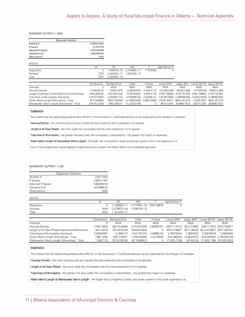
Apples to Apples: A Study of Rural Municipal Finance in Alberta — Technical Appendix
11 | Alberta Association of Municipal Districts & Counties
Regression under 100K AAMDC Municipality Statistical Regression DM
SUMMARY OUTPUT: < 100k
Regression StatisticsMultiple R 0.890153302R Square 0.7923729Adjusted R Square 0.791587948Standard Error 13650489.95Observations 2337
ANOVAdf SS MS F Significance F
Regression 5 1.65833E+18 3.31666E+17 1779.9349 0Residual 2332 4.34535E+17 1.86336E+14Total 2337 2.09286E+18
Coefficients Standard Error t Stat P-value Lower 95% Upper 95% Lower 95.0% Upper 95.0%Intercept 0 #N/A #N/A #N/A #N/A #N/A #N/A #N/AHousing Density -1209288.34 134613.876 -8.98338548 5.2841E-19 -1473263.689 -945312.988 -1473263.69 -945312.988Length of all Open Roads Maintained (Kilometres) 4448.958032 333.4041428 13.34403945 3.3831E-39 3795.158602 5102.757462 3795.158602 5102.757462Total Area of Municipality (Hectares) 4.653778493 0.424891722 10.95285752 2.9346E-27 3.820573593 5.486983394 3.820573593 5.486983394Water Mains Length (Kilometres) - Total -815.839563 4803.762849 -0.169833439 0.86515586 -10235.93071 8604.251579 -10235.9307 8604.251579Wastewater Mains Length (Kilometres) - Total 378191.2246 7383.326141 51.22233766 0 363712.657 392669.7923 363712.657 392669.7923
Explanation
This means that the relationship predicts about 95.5% in the fluctuation in Total Expenditures can be explained by the change in 5 variables:
Housing Density - the more housing units per hectare the less expensive the municipality is to operate.
Length of all Open Roads - the more roads the municipality has the more expensive it is to operate.
Total Area of Municipality - the greater the area under the municipality's responsibility ; the greater the impact on expenses.
Water Mains Length & Wastewater Mains Length - the larger the municipality's water and sewer system is the more expensive it is.
Four of the variable have a good degree of significance (low p-value) with Water Mains not considered significant.
SUMMARY OUTPUT: < 10k
Regression StatisticsMultiple R 0.9111053R Square 0.83011287Adjusted R Square 0.82929318Standard Error 3475966.04Observations 2054
ANOVAdf SS MS F Significance F
Regression 5 1.20968E+17 2.41936E+16 2002.38975 0Residual 2049 2.47567E+16 1.20823E+13Total 2054 1.45724E+17
Coefficients Standard Error t Stat P-value Lower 95% Upper 95% Lower 95.0% Upper 95.0%Intercept 0 #N/A #N/A #N/A #N/A #N/A #N/A #N/AHousing Density 17067.8595 38419.34985 0.444251648 0.65690757 -58277.18722 92412.9062 -58277.1872 92412.90617Length of all Open Roads Maintained (Kilometres) 4815.0218 103.2276106 46.64470846 0 4612.579827 5017.46378 4612.579827 5017.463781Total Area of Municipality (Hectares) 2.63803997 0.1689112 15.61791023 4.8686E-52 2.30678443 2.9692955 2.30678443 2.9692955Water Mains Length (Kilometres) - Total 1564.7236 1297.270971 1.206165583 0.2278929 -979.383533 4108.83073 -979.383533 4108.830728Wastewater Mains Length (Kilometres) - Total 179627.53 3978.206785 45.15288913 0 171825.7796 187429.28 171825.7796 187429.2803
Explanation
This means that the relationship predicts about 95.5% in the fluctuation in Total Expenditures can be explained by the change in 5 variables:
Housing Density - the more housing units per hectare the less expensive the municipality is to operate.
Length of all Open Roads - the more roads the municipality has the more expensive it is to operate.
Total Area of Municipality - the greater the area under the municipality's responsibility ; the greater the impact on expenses.
Water Mains Length & Wastewater Mains Length - the larger the municipality's water and sewer system is the more expensive it is.

Apples to Apples: A Study of Rural Municipal Finance in Alberta — Technical Appendix
12 | Alberta Association of Municipal Districts & Counties
Chart 17: Population versus Asset as a Predictor of Municipal Expenses The data used in the regression analysis comes from the Municipal Financial Information System stewarded by Alberta Municipal Affairs. Data was pulled for population, total expenditures and the value of assets (roads, total hectares, water main length, wastewater main length, and housing density) in each municipality. Two regressions were performed on this data. The first one was a single variable regression with population on total expenditures. This was performed on: All, <100k (this equates to eliminating Edmonton and Calgary), and <10k population municipalities. This same procedure was performed forming regressions using the different asset groups on total expenditures.
Data Types:
• Population – Schedule POPL, column Population• Total Expenditures - Schedule D-total, acct # 2140• Housing Density - Schedule ST-general statistics, acct # 05595• Length of Open Roads Maintained (km) – Schedule ST-general statistics, acct # 05520• Total Area of Municipality (Hectares) – Schedule ST-general statistics, acct # 05510• Water Mains Length (km) – Schedule ST-general statistics, acct # 05560 • Wastewater Mains Length (km) - Schedule ST-general statistics, acct # 05570
In total, six regressions were completed, outputting full sets of regression statistics and analysis of variance (ANOVA) figures. The findings and explanations were subsequently built off of these statistics.
For clarity and visual representation, scatterplots were built for each single variable “population vs. total expenditures” regression. These two data columns were graphed against each other to form the charts further below.
SUMMARY OUTPUT: All Municipalities
Regression StatisticsMultiple R 0.97721632R Square 0.95495174Adjusted R Square 0.95444931Standard Error 35571734.9Observations 2354
ANOVAdf SS MS F Significance F
Regression 5 6.30081E+19 1.26016E+19 9959.01457 0Residual 2349 2.9723E+18 1.26535E+15Total 2354 6.59804E+19
Coefficients Standard Error t Stat P-value Lower 95% Upper 95% Lower 95.0% Upper 95.0%Intercept 0 #N/A #N/A #N/A #N/A #N/A #N/A #N/AHousing Density -2699312.8 328168.0652 -8.22539749 3.1823E-16 -3342841.939 -2055783.62 -3342841.94 -2055783.62Length of all Open Roads Maintained (Kilometres) 3454.0308 861.706826 4.00835957 6.3047E-05 1764.245818 5143.815788 1764.245818 5143.815788Total Area of Municipality (Hectares) 3.77875949 1.071001588 3.528248265 0.00042635 1.678552849 5.878966138 1.678552849 5.878966138Water Mains Length (Kilometres) - Total 27993.4667 11526.55695 2.428606117 0.01523158 5390.184177 50596.74929 5390.184177 50596.74929Wastewater Mains Length (Kilometres) - Total 495388.855 13050.40827 37.95964424 2.663E-246 469797.3393 520980.3711 469797.3393 520980.3711
Explanation
This means that the relationship predicts about 95.5% in the fluctuation in Total Expenditures can be explained by the change in 5 variables:
Housing Density - the more housing units per hectare the less expensive the municipality is to operate.
Length of all Open Roads - the more roads the municipality has the more expensive it is to operate.
Total Area of Municipality - the greater the area under the municipality's responsibility ; the greater the impact on expenses.
Water Mains Length & Wastewater Mains Length - the larger the municipality's water and sewer system is the more expensive it is.

Apples to Apples: A Study of Rural Municipal Finance in Alberta — Technical Appendix
13 | Alberta Association of Municipal Districts & Counties
3,000,000,000
2,500,000,000
2,000,000,000
1,500,000,000
1,000,000,000
500,000,000
0
3,500,000,000
200,000 400,000 600,000 800,000 1,000,000 1,200,000
R2 = 0.9608
To
tal E
xpen
dit
ure
s
Population
Relationship between Alberta Municipal Population and Total Expenditures – All Municipalities 2004 – 2011
300,000,000
250,000,000
200,000,000
150,000,000
100,000,000
50,000,000
0
350,000,000
20,000 40,000 60,000 80,000 100,000 120,000
R2 = 0.8057
To
tal E
xpen
dit
ure
s
Population
400,000,000
450,000,000
500,000,000
Relationship between Alberta Municipal Population and Total Expenditures – Excluding Edmonton & Calgary
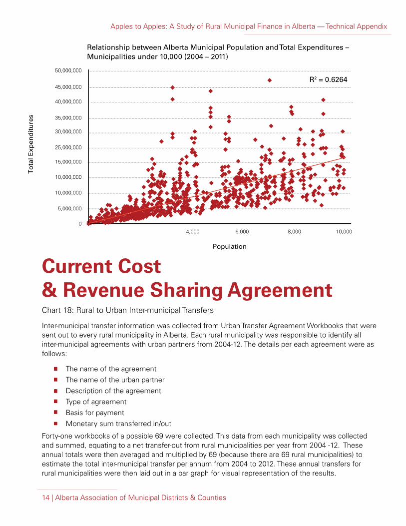
Apples to Apples: A Study of Rural Municipal Finance in Alberta — Technical Appendix
14 | Alberta Association of Municipal Districts & Counties
Relationship between Alberta Municipal Population and Total Expenditures – Municipalities under 10,000 (2004 – 2011)
30,000,000
25,000,000
15,000,000
10,000,000
10,000,000
5,000,000
0
35,000,000
4,000 6,000 8,000 10,000
R2 = 0.6264
To
tal E
xpen
dit
ure
s
Population
40,000,000
45,000,000
50,000,000
Chart 18: Rural to Urban Inter-municipal Transfers
Inter-municipal transfer information was collected from Urban Transfer Agreement Workbooks that were sent out to every rural municipality in Alberta. Each rural municipality was responsible to identify all inter-municipal agreements with urban partners from 2004-12. The details per each agreement were as follows:
• The name of the agreement• The name of the urban partner• Description of the agreement• Type of agreement• Basis for payment• Monetary sum transferred in/out
Forty-one workbooks of a possible 69 were collected. This data from each municipality was collected and summed, equating to a net transfer-out from rural municipalities per year from 2004 -12. These annual totals were then averaged and multiplied by 69 (because there are 69 rural municipalities) to estimate the total inter-municipal transfer per annum from 2004 to 2012. These annual transfers for rural municipalities were then laid out in a bar graph for visual representation of the results.
Current Cost & Revenue Sharing Agreement
Apples to Apples: A Study of Rural Municipal Finance in Alberta — Technical Appendix
15 | Alberta Association of Municipal Districts & Counties
Regression Analysis Overview Regression analysis is a statistical process for estimating the relationship among variables, focusing on the relationship between one dependent variable (municipal expenditure) and a number of independent variables (population, housing density, length of all open roads maintained, total area of municipality, water mains length, and wastewater mains length.) Regression analysis is used to understand which among the independent variables are related to the dependent variable, which is used to infer if causal relationships exist between the dependent variable and certain independent variables. Causality is the relation between an event – ‘the cause’ – and a second event –‘the effect’- where the second event is understood as a consequence of the first. In basic terms, regression analysis discovers the power of certain independent variable in explaining the changes of the dependent variable.
While the seemingly whimsical statistics computed from a regression analysis are complicated, the deductions that can be drawn from them are surprisingly simple. In our regression analysis, we use three core factors which we subsequently deduce our findings. They are:
i. Coefficient of Determination: denoted as R2, the coefficient of determination specifies how well the data points fit a line or curve; how accurate a line of best fit is. In simplest terms, the R2 value is a measure of the accuracy (where 100% is perfect correlation) of the model in replicating the observed outcomes, in the form of the proportion of the total variation of outcomes explained by the model. If the R2 value is 1.00, the independent variables explain the dependent variable outcomes with perfect accuracy. The higher the R2 value, the more explanatory power the independent variable has in predicting the dependent variable. A real life example would be a data set of human beings with weight as the dependent variable and height as the independent variable. It is logical that a strong correlation exists and thus presumably the R2 value will be very high. In comparison, if the dependent variable was weight and the independent variable was your IQ, the correlation between these variable is presumably quite low and thus the R2 is low.
ii. P-value: is the probability of obtaining a test statistic at least as extreme as the one that was actually observed, assuming that the null hypothesis is true. The null hypothesis is often rejected when the p-value is less than a predetermined significance level, normally 0.05 or 0.01. If the p-value is less than the significance level, and null hypothesis is rejected, indicating that the observed result is highly unlikely due to random chance; meaning that causality between the independent and dependent variables exists. In a nutshell, the lower the p-value, the stronger the proof that a causal relationship exists between dependent and independent variable.
Appendix
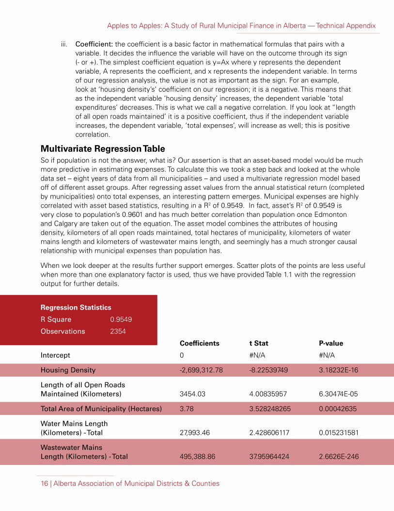
Apples to Apples: A Study of Rural Municipal Finance in Alberta — Technical Appendix
16 | Alberta Association of Municipal Districts & Counties
iii. Coefficient: the coefficient is a basic factor in mathematical formulas that pairs with a variable. It decides the influence the variable will have on the outcome through its sign (- or +). The simplest coefficient equation is y=Ax where y represents the dependent variable, A represents the coefficient, and x represents the independent variable. In terms of our regression analysis, the value is not as important as the sign. For an example, look at ‘housing density’s’ coefficient on our regression; it is a negative. This means that as the independent variable ‘housing density’ increases, the dependent variable ‘total expenditures’ decreases. This is what we call a negative correlation. If you look at “length of all open roads maintained’ it is a positive coefficient, thus if the independent variable increases, the dependent variable, ‘total expenses’, will increase as well; this is positive correlation.
Multivariate Regression Table So if population is not the answer, what is? Our assertion is that an asset-based model would be much more predictive in estimating expenses. To calculate this we took a step back and looked at the whole data set – eight years of data from all municipalities – and used a multivariate regression model based off of different asset groups. After regressing asset values from the annual statistical return (completed by municipalities) onto total expenses, an interesting pattern emerges. Municipal expenses are highly correlated with asset based statistics, resulting in a R2 of 0.9549. In fact, asset’s R2 of 0.9549 is very close to population’s 0.9601 and has much better correlation than population once Edmonton and Calgary are taken out of the equation. The asset model combines the attributes of housing density, kilometers of all open roads maintained, total hectares of municipality, kilometers of water mains length and kilometers of wastewater mains length, and seemingly has a much stronger causal relationship with municipal expenses than population has.
When we look deeper at the results further support emerges. Scatter plots of the points are less useful when more than one explanatory factor is used, thus we have provided Table 1.1 with the regression output for further details.
Regression Statistics
R Square 0.9549
Observations 2354
Coefficients t Stat P-value
Intercept 0 #N/A #N/A
Housing Density -2,699,312.78 -8.22539749 3.18232E-16
Length of all Open Roads Maintained (Kilometers) 3454.03 4.00835957 6.30474E-05
Total Area of Municipality (Hectares) 3.78 3.528248265 0.00042635
Water Mains Length (Kilometers) - Total 27,993.46 2.428606117 0.015231581
Wastewater Mains Length (Kilometers) - Total 495,388.86 37.95964424 2.6626E-246
Apples to Apples: A Study of Rural Municipal Finance in Alberta — Technical Appendix
17 | Alberta Association of Municipal Districts & Counties
When reading the results there are three important areas to focus on, as previously highlighted. These are the R2, the coefficients and the P-value. The R2 value has been described and explained above. The coefficients predict how much each of the variables contributes to the total expenses per unit; that is, how much expense is associated with a kilometer of road. In most cases, the value of the coefficient is not as important as the sign (+ or -) in interpreting the analysis.
Four of the five asset groups have positive coefficients and thus have follow an intuitive pattern than having more assets means increased costs to build and maintain. The last factor, ‘housing density’, has a negative coefficient and thus a negative correlation with total expenses. This is evidence that the more condensed a municipality is, the lower the costs on a per house basis to service. This is the logical argument against urban sprawl; the more spread out a population base is the more expensive it is to service them. This argument has been sited against urban sprawl in other cases.
Reporting Changes Starting in 2009, major accounting changes from the Public Sector Accounting Board (PSAB) took place, especially regarding Tangible Capital Assets (TCA). Beginning January 1, 2009 all governments used the same financial reporting model which utilizes accrual accounting. PSAB reporting provides highly comprehensive financial statements that focus equally between the annual surplus/deficit and the overall financial health of the municipality.
There are five major changes under the new PSAB accounting standards:
1. TCA/Amortization: Capital payments are now recorded as TCA’s and amortized over its useful life instead of directly being expensed in the period.
2. Accrual Accounting: Accounting has moved from a modified cash basis where expenditures are recorded when cash is disbursed to an accrual system when expenses are recorded as incurred (accrued salaries, accounts payable, environmental liabilities.)
3. Debt Payments: Under the old cash basis system, debt service charges included interest and principal payments and the total was then expensed. Under the new accrual system debt service charges (expenses) only include interest and the principal payments reduce the liability.
4. Reporting Entity: Under the old system the financial statements only reported on the activities of the municipality. Each of the three funds (general operating fund, reserves, and general capital fund) is presented separately on the financial statements. Under the new PSAB system, the financial statements includes all organizations that are controlled by the municipality. Having control means having the power to govern, the authority to determine financial and operating policies and responsible for expected benefits or risk of loss, hold the majority of voting shares, and/or unilateral power to dissolve the organization. The controlled organizations/government partnerships are consolidated into one set of summary financial statements.
5. Transfers: Under the old system, inter-fund and inter-organization balances and transactions were recorded. Now, these transactions are not recorded and transfers to reserves are not classified as expenses and transfers from reserves are not classified as revenues.
Pre 2009, any surplus in the operating fund at the end of the year was transferred to reserve accounts to be used in future periods to offset future revenue requirements.