1

Appendix K: Price Elasticity of Demand

General Elasticity Theory

(i) Definition and Types of Elasticity

Standard economic theory dictates that customers react to changes in prices by adjusting their demand for the

goods in question. As prices rise, customers reduce the quantity demanded. As prices drop, customers increase

the quantity demanded. The responsiveness of customers to price changes is called their price elasticity of

demand.

The own price elasticity of demand is simply the percentage change in consumption due to a one percentage

change in price. For example, if price doubles - an increase of 100 percent - and usage declines by 30 percent,

then the own price elasticity equals -30 percent/100 percent, or -0.30. Elasticities are expressed as fractions

and have no units.

Price elasticity of demand is therefore given by the following formulae:

price

quantity

%

%

For a price increase along a demand curve from price 0P to 1P , the elasticity can be calculated from the

corresponding change in quantity, using the averages of prices and quantities, from:

01

01

21

1

PaverageP

PP

QaverageQ

QQ o

In terms of its application to electricity demand, the own price elasticity of electricity typically measures the

change in energy consumption arising from a change in energy price. The primary measure of interest is the

change in peak period energy consumption caused by a change in peak energy price (own price elasticity: peak

energy), usually as a result of a shift to a ToU or Critical Peak Price (CPP) structure. However, the change in

off-peak energy stemming from a change in off-peak price (own price elasticity: off-peak energy) may also be of

interest.

The own price elasticity of electricity demand may also be calculated as the change in coincident peak demand

arising from a change in peak energy price (own price elasticity: peak demand). However, as the preliminary

results of the Californian Statewide Pricing Pilot (SPP) showed (discussed later on), these values are very

similar to (and arguably interchangeable with) the own price elasticity- peak energy estimates. It is often easier

to work with consumption rather than demand, as this avoids the need to estimate coincidence and diversity

factors when applying elasticity estimates.

In general, the cross price elasticity of demand measures the change in demand for one product caused by the

change in price of another:

Y

Xcrossprice

price

quantity

%

%

If two goods are substitutes (compliments), their cross price elasticity of demand is positive (negative).

In relation to electricity demand, there are two possible applications of cross price elasticities:

Cross price elasticity: peak/off-peak - the change in peak (off-peak) consumption resulting from a change

in the off-peak (peak) price; or

Cross price elasticity: gas (or other fuel source) - the change in electricity consumption resulting from a

change in the price of a potential substitute fuel source (such as natural gas).

2

Taking the cross price elasticity: peak/off-peak, a positive (negative) cross price elasticity means that peak and

off-peak energy consumption are substitutes (compliments) – i.e. as peak price increases, off-peak energy

consumption increases (decreases).

Intuitively, you would expect that an increase in the off-peak price would result in a decrease in peak period

consumption as well as off-peak consumption (as the peak price would most likely be even higher). Peak

consumption would therefore have a negative cross price elasticity with off-peak price (peak and off-peak

periods are complimentary).

An increase in the peak price could result in an increase in off-peak consumption, along with a decrease in peak

period consumption, as customers shift usage to cheaper time periods. This would result in a positive cross

price elasticity of off-peak consumption with peak price (peak and off-peak periods are substitutes). If the price

elasticity of off-peak consumption with peak price was negative (peak and off are compliments), this would imply

energy conservation from a peak price increase, as opposed to substituting usage to cheaper time periods.

The cross price elasticity of electricity with gas is likely to be positive - if the gas price increases then electricity

consumption will increase, as most domestic gas applications have a corresponding electricity option (e.g.

cooking, space heating). The cross price elasticity of gas with electricity is likely to be lower – if the electricity

price rises, customers can only substitute gas appliances for certain applications – there are limited practical

substitutes for applications such as internal lighting.

A closely related measure to the cross price elasticity, although measured via a different equation, is the

elasticity of substitution. In the case of electricity demand, this measures the percentage shift in a customer’s

consumption across time periods (such as peak to off-peak) in response to price changes that alter the price

relationship between the two time periods (e.g. changing the price ratio from 1:1 to 2:1). For example, in the

case of a ToU rate, the peak to off-peak elasticity of substitution represents the percentage change in the ratio

of peak to off-peak usage that occurs in response to a given change in the ratio of peak to off-peak prices, all

other factors held constant.

An elasticity of substitution value of 0.10 implies that a peak to off-peak price ratio of 150 percent (e.g. with peak

and off-peak prices of $0.25 and $0.10/kWh respectively, and calculating the percent change as the natural

logarithm of the price ratio) will produce a reduction in peak to off-peak usage of 15 percent relative to the case

for a flat price (i.e., -0.10 * 150 percent = -15 percent).

In economic terms, the elasticity of substitution measures the shape of the indifference curves that underlie the

consumer’s utility function. It is related to the own price and cross price elasticities of demand through the

Slutsky equation in microeconomics:

Own price elasticity of demand = compensated own price elasticity of demand + (income elasticity of

demand * budget share of commodity in question).

Hence own price elasticities and substitution elasticities may be compared when the necessary data are

available. Caves and Christensen (1980) showed that an elasticity of substitution of 0.17 was consistent with a

peak-period own-price elasticity of approximately -0.30.

(ii) Properties of Elasticity

Elasticity estimates can be classified as either elastic or inelastic. Generally, a demand response is referred to

as being elastic (or highly elastic) if the elasticity is greater than 1, i.e. if a 1% change in price corresponds to a

greater than 1% change in quantity. Conversely, a demand response is referred to as being inelastic if the

elasticity is less than 1, i.e. if a 1% change in price corresponds to a less than 1% change in quantity. A unit

elastic demand response occurs where a 1% change in price results in a 1% change in quantity.

3

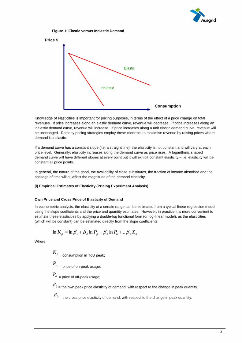
Figure 1: Elastic versus Inelastic Demand

Knowledge of elasticities is important for pricing purposes, in terms of the effect of a price change on total

revenues. If price increases along an elastic demand curve, revenue will decrease. If price increases along an

inelastic demand curve, revenue will increase. If price increases along a unit elastic demand curve, revenue will

be unchanged. Ramsey pricing strategies employ these concepts to maximise revenue by raising prices where

demand is inelastic.

If a demand curve has a constant slope (i.e. a straight line), the elasticity is not constant and will vary at each

price level. Generally, elasticity increases along the demand curve as price rises. A logarithmic shaped

demand curve will have different slopes at every point but it will exhibit constant elasticity – i.e. elasticity will be

constant all price points.

In general, the nature of the good, the availability of close substitutes, the fraction of income absorbed and the

passage of time will all affect the magnitude of the demand elasticity.

(i) Empirical Estimates of Elasticity (Pricing Experiment Analysis)

Own Price and Cross Price of Elasticity of Demand

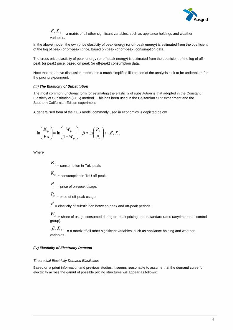
In econometric analysis, the elasticity at a certain range can be estimated from a typical linear regression model

using the slope coefficients and the price and quantity estimates. However, in practice it is more convenient to

estimate these elasticities by applying a double-log functional form (or log-linear model), as the elasticities

(which will be constant) can be estimated directly from the slope coefficients:

nnopp XPPK ...lnlnlnln 321

Where:

pK= consumption in ToU peak;

pP = price of on-peak usage;

oP = price of off-peak usage;

2 = the own peak price elasticity of demand, with respect to the change in peak quantity.

3 = the cross price elasticity of demand, with respect to the change in peak quantity.

Price $

Elastic

Inelastic

Consumption

4

nn X = a matrix of all other significant variables, such as appliance holdings and weather

variables.

In the above model, the own price elasticity of peak energy (or off-peak energy) is estimated from the coefficient

of the log of peak (or off-peak) price, based on peak (or off-peak) consumption data.

The cross price elasticity of peak energy (or off peak energy) is estimated from the coefficient of the log of off-

peak (or peak) price, based on peak (or off-peak) consumption data.

Note that the above discussion represents a much simplified illustration of the analysis task to be undertaken for

the pricing experiment.

(iii) The Elasticity of Substitution

The most common functional form for estimating the elasticity of substitution is that adopted in the Constant

Elasticity of Substitution (CES) method. This has been used in the Californian SPP experiment and the

Southern Californian Edison experiment.

A generalised form of the CES model commonly used in economics is depicted below.

nn

o

p

p

ppX

P

P

W

W

Ko

K ..ln

1lnln

Where

pK= consumption in ToU peak;

oK = consumption in ToU off-peak;

pP = price of on-peak usage;

oP = price of off-peak usage;

= elasticity of substitution between peak and off-peak periods.

pW = share of usage consumed during on-peak pricing under standard rates (anytime rates, control

group).

nn X = a matrix of all other significant variables, such as appliance holding and weather

variables.

(iv) Elasticity of Electricity Demand

Theoretical Electricity Demand Elasticities

Based on a priori information and previous studies, it seems reasonable to assume that the demand curve for

electricity across the gamut of possible pricing structures will appear as follows:

5

Figure 2: Electricity Demand Curve and Elasticity Ranges

As shown above, at lower price levels (such as the Inclining Block Tariff (IBT) level), a price rise is unlikely to

produce a significant change in demand. This is because the price level is very low and represents a small

proportion of the household budget. In addition, the three-month information delay effect from accumulation

meters will further stifle behaviour change.

If the customer is then placed on a ToU or seasonal tariff with a significant change to the peak price, there will

be a noticeable change in behaviour and the percentage change in volume will be high compared to the change

in price (hence the elasticity will be larger).

However, as the price moves into the CPP realm, there is likely to be a limit on the extent to which customers

are able to change peak consumption. Therefore, even though a CPP price rise will result in a greater reduction

in peak demand than under the ToU rate, the reduction compared to the percentage change in price could be

less, resulting in a lower elasticity value (the longer term effect may be greater).

(iv) Factors Influencing Electricity Price Elasticity of Demand

The magnitude of the price change

The principal determinant of demand response to a price signal is the magnitude of the price change itself. A

change in price will result in a movement along the electricity demand curve – a change in other non-price

variables (such as an increase in disposable income) will result in a shift of the demand curve.

Price elasticity of electricity demand is unlikely to be constant for varying magnitudes of changes in price (i.e. it

may be non-linear). The magnitude of the price change will affect the price elasticity of demand since small

price changes are likely to elicit only minor adjustment to customer behaviour while large changes may instigate

changes to stocks of electric devices or more radical behavioural change.

Dynamic Pricing (e.g. CPP, RTP)

Dynamic pricing refers to tariff structures that recognise uncertainty and high cost events in wholesale supply

costs and network provision of services, including real time pricing (RTP) and critical peak pricing (CPP). Price

levels and time periods are variable over short periods of time.

At high peak price levels, electricity costs represent a larger proportion of household expenditure or business

input costs, therefore consumers are more likely to adjust behaviour to minimise costs. However, there is likely

to be a threshold level – for price rises above this level, consumers will not be able to reduce any further peak

demand consumption as there is no more discretionary load available. The demand curve will become

Po -IBT

P1 IBT rise

P2 ToU

P4 CPP

Peak price - $/kWh

Co -IBT C1 IBT rise C2 ToU C4 CPP

Elastic

Inelastic (insufficient price signal to change consumption)

Inelastic (diminishing returns)

P3 Seasonal

C3 Seasonal

6

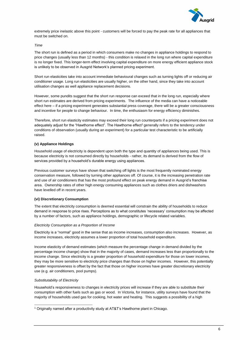
extremely price inelastic above this point - customers will be forced to pay the peak rate for all appliances that

must be switched on.

Time

The short run is defined as a period in which consumers make no changes in appliance holdings to respond to

price changes (usually less than 12 months) - this condition is relaxed in the long run where capital expenditure

is no longer fixed. This longer-term effect involving capital expenditure on more energy efficient appliance stock

is unlikely to be observed in Ausgrid Network’s planned pricing experiment.

Short run elasticities take into account immediate behavioural changes such as turning lights off or reducing air

conditioner usage. Long run elasticities are usually higher, on the other hand, since they take into account

utilisation changes as well appliance replacement decisions.

However, some pundits suggest that the short run response can exceed that in the long run, especially where

short run estimates are derived from pricing experiments. The influence of the media can have a noticeable

effect here – if a pricing experiment generates substantial press coverage, there will be a greater consciousness

and incentive for people to change behaviour. In time, the enthusiasm for energy efficiency diminishes.

Therefore, short run elasticity estimates may exceed their long run counterparts if a pricing experiment does not

adequately adjust for the “Hawthorne effect”. The Hawthorne effect1 generally refers to the tendency under

conditions of observation (usually during an experiment) for a particular test characteristic to be artificially

raised.

(v) Appliance Holdings

Household usage of electricity is dependent upon both the type and quantity of appliances being used. This is

because electricity is not consumed directly by households - rather, its demand is derived from the flow of

services provided by a household’s durable energy using appliances.

Previous customer surveys have shown that switching off lights is the most frequently nominated energy

conservation measure, followed by turning other appliances off. Of course, it is the increasing penetration rate

and use of air conditioners that has the most profound effect on peak energy demand in Ausgrid’s franchise

area. Ownership rates of other high energy consuming appliances such as clothes driers and dishwashers

have levelled off in recent years.

(vi) Discretionary Consumption

The extent that electricity consumption is deemed essential will constrain the ability of households to reduce

demand in response to price rises. Perceptions as to what constitutes ‘necessary’ consumption may be affected

by a number of factors, such as appliance holdings, demographic or lifecycle related variables.

Electricity Consumption as a Proportion of Income

Electricity is a “normal” good in the sense that as income increases, consumption also increases. However, as

income increases, electricity assumes a lower proportion of total household expenditure.

Income elasticity of demand estimates (which measure the percentage change in demand divided by the

percentage income change) show that in the majority of cases, demand increases less than proportionally to the

income change. Since electricity is a greater proportion of household expenditure for those on lower incomes,

they may be more sensitive to electricity price changes than those on higher incomes. However, this potentially

greater responsiveness is offset by the fact that those on higher incomes have greater discretionary electricity

use (e.g. air conditioners, pool pumps).

Substitutability of Electricity

Household’s responsiveness to changes in electricity prices will increase if they are able to substitute their

consumption with other fuels such as gas or wood. In Victoria, for instance, utility surveys have found that the

majority of households used gas for cooking, hot water and heating. This suggests a possibility of a high

1 Originally named after a productivity study at AT&T’s Hawthorne plant in Chicago.

7

degree of substitutability of electricity for certain activities, yet for other purposes such as lighting or electrical

appliance usage there will be little or no substitutability.

This form of substitutability is only evident in the long run, where appliance stock is able to change.

Information

Customers with a Type 6 accumulation meter on an IBT only receive information on their electricity usage and

cost via their bill, which for Ausgrid is issued every three months. This lag between behaviour and the price

signal will dampen the response rate to a price change.

In contrast, previous CPP trials have incorporated in-house display units linked to the “smart” meter. These

units provide a host of information including tariff rates, average price (including the effect of switching off

appliances on average price), consumption, and technical specifications. A trial conducted by Northern Ireland

Electricity, undertaken in conjunction with pre-payment meters, showed that customers on a IBT structure

reduced consumption by 11% purely through the installation of in-house display units (i.e. with no change to

their existing tariff). This figure reduced to 4% when a larger-scale rollout was completed, but this still highlights

the potential influence of information on price responsiveness.

The media can also exert a strong influence on price responsiveness through raising customers’ awareness of

energy conservation issues. Also, if a pricing experiment were to receive significant media coverage, this could

raise the short run elasticity above the true equilibrium rate.

However, the SPP experiment highlighted the importance of price signals in eliciting demand reductions, as the

available of information on its own does not tend to produce sustainable load shifting behaviour.

(vii) Summary of Australian Studies of Elasticity of Electricity Demand Studies

NIEIR Estimates

NEMMCO commissioned the National Institute of Economic and Industry Research (NIEIR) in 2002 to provide

advice on the long run price elasticity of demand for electricity in the NEM region, as part of the preparation of

the 2002 Statement of Opportunities. Based upon a review of overseas and Australian literature, using data

from 1980 to 1995, NIEIR (2002) recommended the following long run elasticities of demand in Australia:

Residential -0.25

Commercial -0.35

Industrial -0.38

It is interesting that in the long run, the commercial and industrial estimates for Australia are higher than the

residential sector. This is in contrast to the view held by some that, in the short run, residential own price

elasticities exceed the commercial and industrial values.

It is understood that these estimates could be taken to indicate the change in peak energy consumption likely to

result from a given change in peak price.

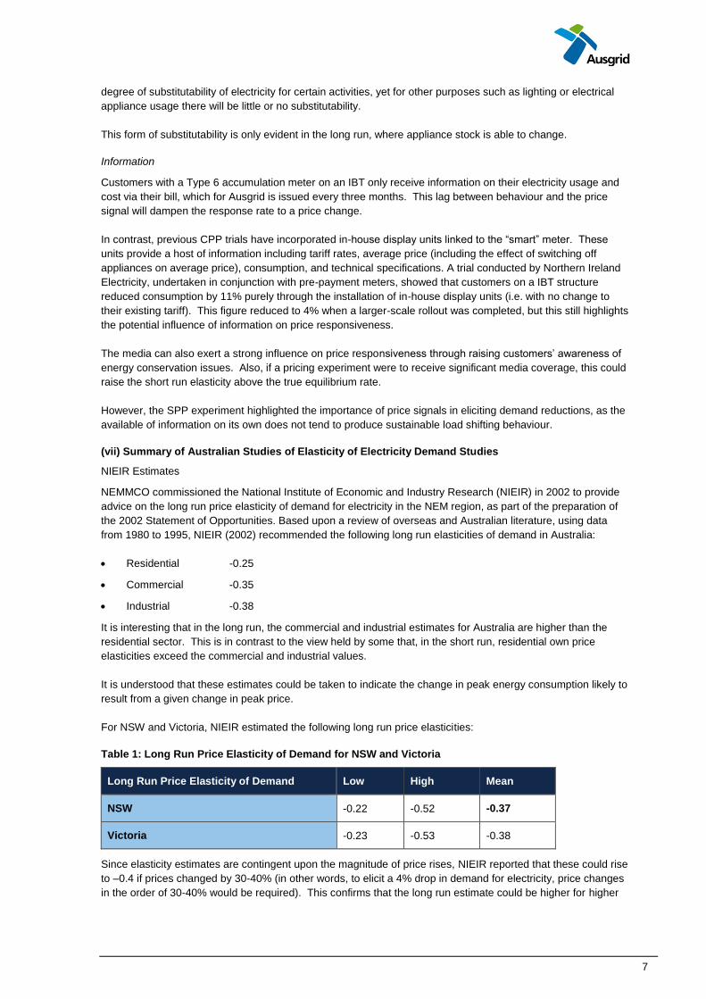
For NSW and Victoria, NIEIR estimated the following long run price elasticities:

Table 1: Long Run Price Elasticity of Demand for NSW and Victoria

Long Run Price Elasticity of Demand Low High Mean

NSW -0.22 -0.52 -0.37

Victoria -0.23 -0.53 -0.38

Since elasticity estimates are contingent upon the magnitude of price rises, NIEIR reported that these could rise

to –0.4 if prices changed by 30-40% (in other words, to elicit a 4% drop in demand for electricity, price changes

in the order of 30-40% would be required). This confirms that the long run estimate could be higher for higher

8

peak price structures. However, the NIEIR study has not shed light on the issue of a “cap” on maximum

demand response, which would require a lower elasticity at high critical peak rates.

Akmal and Stern (2001)

Using ABS data from 1969 to 1999, Akmal and Stern (2001) examined the residential price elasticity of demand

across all types of energy in Australia. For electricity, they estimate a long run elasticity of -0.95. Akmal and

Stern (2001) also report values from other Australian studies (mainly produced in the 1980s using data from

1960 to 1982). These studies estimated elasticities in the range –0.55 to –0.86. These results appear to be

unusually high.

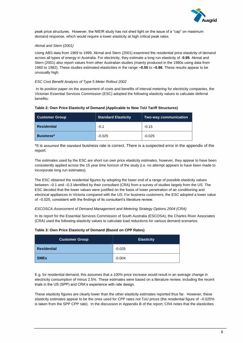
ESC Cost Benefit Analysis of Type 5 Meter Rollout 2002

In its position paper on the assessment of costs and benefits of interval metering for electricity companies, the

Victorian Essential Services Commission (ESC) adopted the following elasticity values to calculate deferral

benefits:

Table 2: Own Price Elasticity of Demand (Applicable to New ToU Tariff Structures)

Customer Group Standard Elasticity Two-way communication

Residential -0.1 -0.15

Business* -0.025 -0.025

*It is assumed the standard business rate is correct. There is a suspected error in the appendix of the

report.

The estimates used by the ESC are short run own price elasticity estimates, however, they appear to have been

consistently applied across the 15 year time horizon of the study (i.e. no attempt appears to have been made to

incorporate long run estimates).

The ESC obtained the residential figures by adopting the lower end of a range of possible elasticity values

between –0.1 and –0.3 identified by their consultant (CRA) from a survey of studies largely from the US. The

ESC decided that the lower values were justified on the basis of lower penetration of air conditioning and

electrical appliances in Victoria compared with the US. For business customers, the ESC adopted a lower value

of –0.025, consistent with the findings of its consultant’s literature review.

ESCOSCA Assessment of Demand Management and Metering Strategy Options 2004 (CRA)

In its report for the Essential Services Commission of South Australia (ESCOSA), the Charles River Associates

(CRA) used the following elasticity values to calculate load reductions for various demand scenarios:

Table 3: Own Price Elasticity of Demand (Based on CPP Rates)

Customer Group Elasticity

Residential -0.025

SMEs -0.004

E.g. for residential demand, this assumes that a 100% price increase would result in an average change in

electricity consumption of minus 2.5%. These estimates were based on a literature review, including the recent

trials in the US (SPP) and CRA’s experience with rate design.

These elasticity figures are clearly lower than the other elasticity estimates reported thus far. However, these

elasticity estimates appear to be the ones used for CPP rates not ToU prices (the residential figure of –0.025%

is taken from the SPP CPP rate). In the discussion in Appendix B of the report, CRA notes that the elasticities

9

pertaining to CPP programs are very different to those reported for ToU rates – the latter ranging from –0.2 to –

0.3 (in line with other estimates).

As an illustrative example, if a 5% price increase produces a 1.5% decrease in electricity consumption, elasticity

will be –0.3. However, a price increase in a CPP program of 333%, using the elasticity of –0.3, would result in a

100% peak period reduction. Clearly, this is unlikely. Therefore, to capture the threshold issue, CRA apply

lower price elasticities for CPP.

CRA state that CPP programs to date have resulted in consumption decreases in the order of 10% to 40%,

leading to elasticities in the order of –0.02 to –0.08.

However, it is noted that there are a lot of CPP studies which support CPP elasticity values of a similar

magnitude to those estimated under ToU tariffs – i.e. in the range of –0.1 to –0.3.

AGA Research Paper 1996

The Australian Gas Association (AGA) undertook a study of price elasticities for gas and electricity based on

data from 1973-74 to 1993-94. The AGA computed both long and short run estimates, as well as own price and

cross price elasticities. Note that in this study, cross price elasticities were defined as the percentage change in

the quantity of gas (electricity) demanded in response to a one percent change in the price of electricity (gas).

The price data was based on annual ABARE data, which is comprised largely of flat rate tariff structures for the

residential sector. It seems logical to expect there would be a slight difference in results between this type of

long run study and a short run study such as a pricing experiment, based on higher-priced ToU tariff structures.

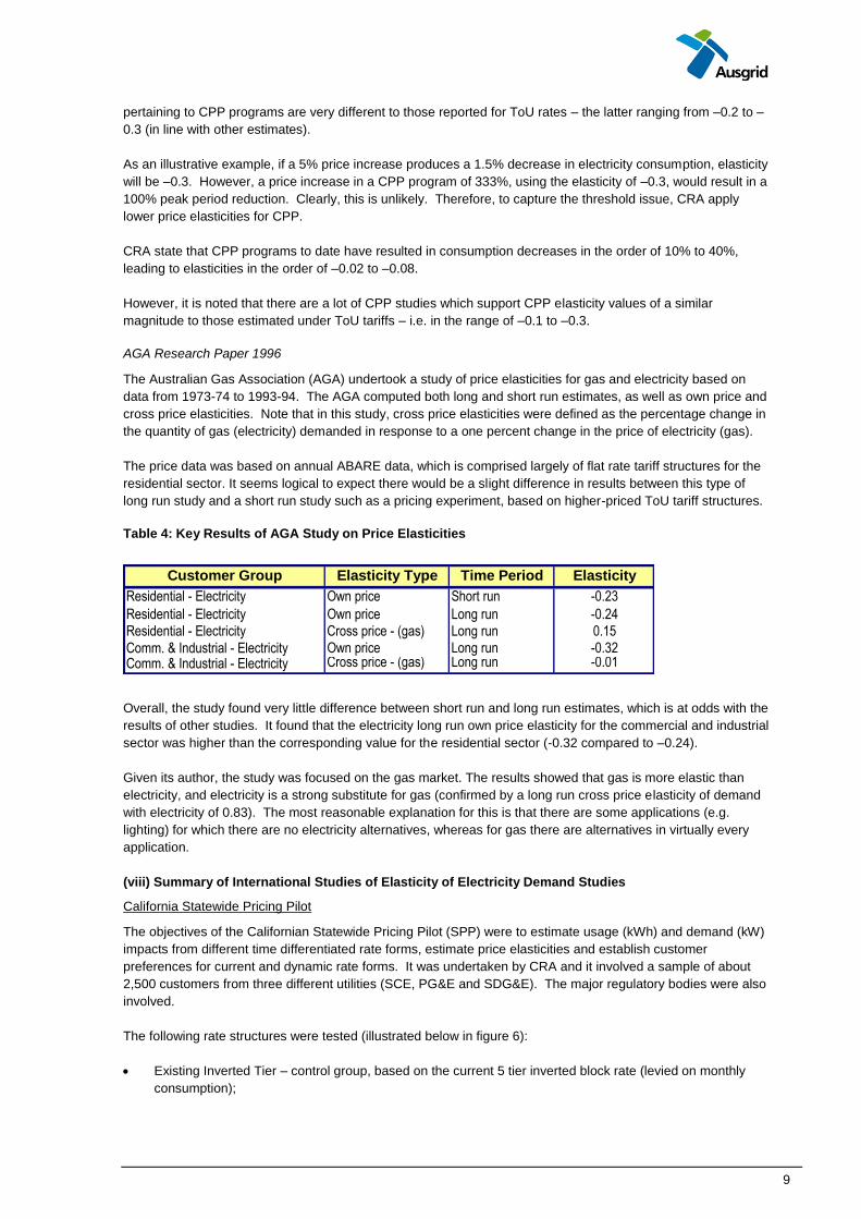
Table 4: Key Results of AGA Study on Price Elasticities

Overall, the study found very little difference between short run and long run estimates, which is at odds with the

results of other studies. It found that the electricity long run own price elasticity for the commercial and industrial

sector was higher than the corresponding value for the residential sector (-0.32 compared to –0.24).

Given its author, the study was focused on the gas market. The results showed that gas is more elastic than

electricity, and electricity is a strong substitute for gas (confirmed by a long run cross price elasticity of demand

with electricity of 0.83). The most reasonable explanation for this is that there are some applications (e.g.

lighting) for which there are no electricity alternatives, whereas for gas there are alternatives in virtually every

application.

(viii) Summary of International Studies of Elasticity of Electricity Demand Studies

California Statewide Pricing Pilot

The objectives of the Californian Statewide Pricing Pilot (SPP) were to estimate usage (kWh) and demand (kW)

impacts from different time differentiated rate forms, estimate price elasticities and establish customer

preferences for current and dynamic rate forms. It was undertaken by CRA and it involved a sample of about

2,500 customers from three different utilities (SCE, PG&E and SDG&E). The major regulatory bodies were also

involved.

The following rate structures were tested (illustrated below in figure 6):

Existing Inverted Tier – control group, based on the current 5 tier inverted block rate (levied on monthly

consumption);

Customer Group Elasticity Type Time Period Elasticity

Residential - Electricity Own price Short run -0.23

Residential - Electricity Own price Long run -0.24Residential - Electricity Cross price - (gas) Long run 0.15

Comm. & Industrial - Electricity Own price Long run -0.32Comm. & Industrial - Electricity Cross price - (gas) Long run -0.01

10

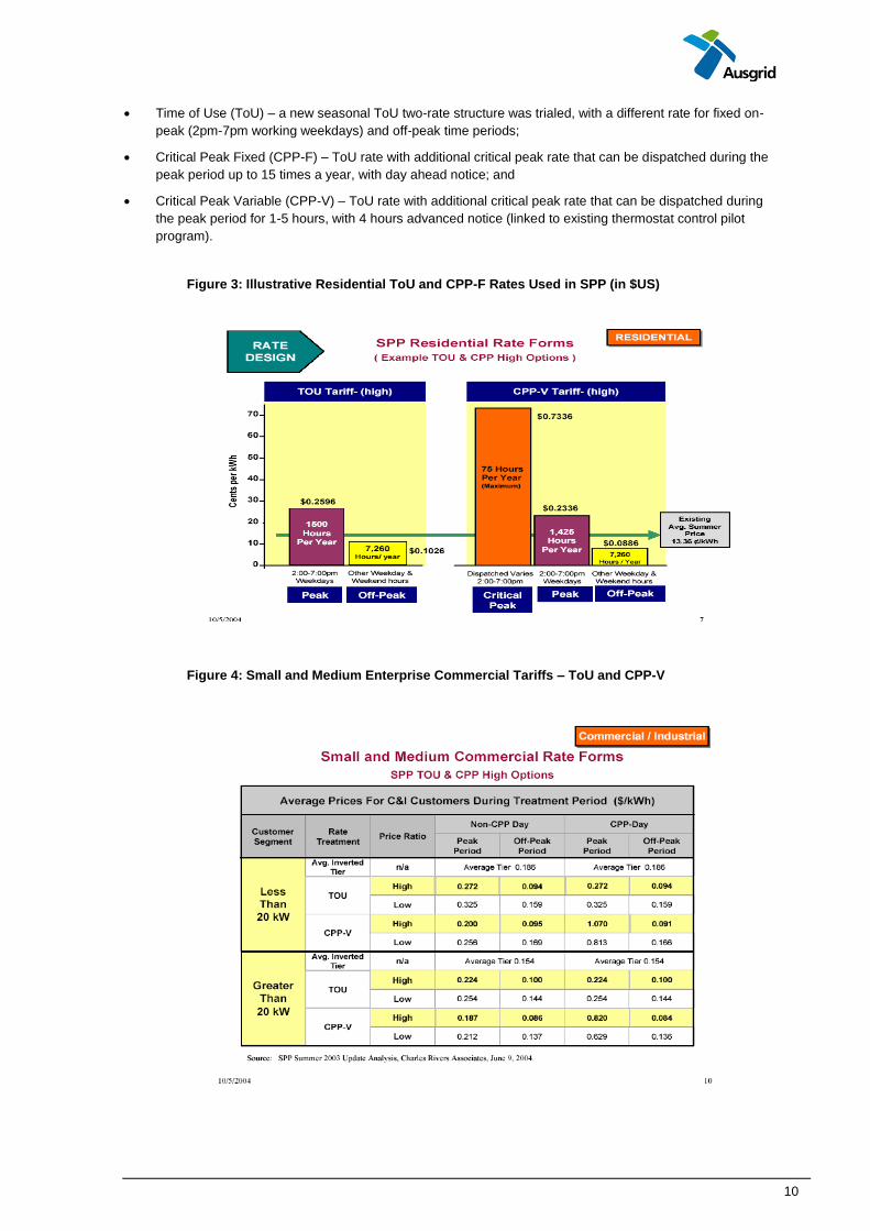
Time of Use (ToU) – a new seasonal ToU two-rate structure was trialed, with a different rate for fixed on-

peak (2pm-7pm working weekdays) and off-peak time periods;

Critical Peak Fixed (CPP-F) – ToU rate with additional critical peak rate that can be dispatched during the

peak period up to 15 times a year, with day ahead notice; and

Critical Peak Variable (CPP-V) – ToU rate with additional critical peak rate that can be dispatched during

the peak period for 1-5 hours, with 4 hours advanced notice (linked to existing thermostat control pilot

program).

Figure 3: Illustrative Residential ToU and CPP-F Rates Used in SPP (in $US)

Figure 4: Small and Medium Enterprise Commercial Tariffs – ToU and CPP-V

11

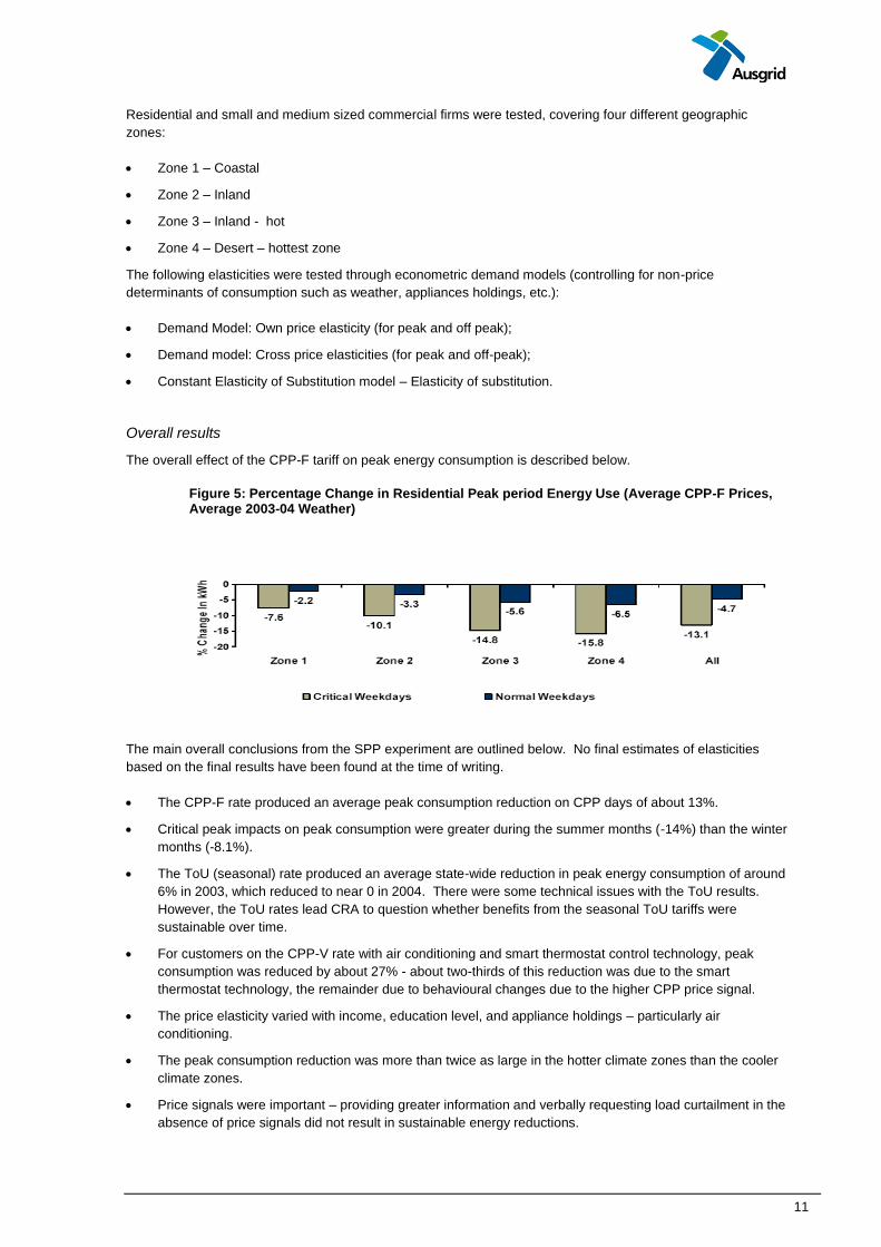
Residential and small and medium sized commercial firms were tested, covering four different geographic

zones:

Zone 1 – Coastal

Zone 2 – Inland

Zone 3 – Inland - hot

Zone 4 – Desert – hottest zone

The following elasticities were tested through econometric demand models (controlling for non-price

determinants of consumption such as weather, appliances holdings, etc.):

Demand Model: Own price elasticity (for peak and off peak);

Demand model: Cross price elasticities (for peak and off-peak);

Constant Elasticity of Substitution model – Elasticity of substitution.

Overall results

The overall effect of the CPP-F tariff on peak energy consumption is described below.

Figure 5: Percentage Change in Residential Peak period Energy Use (Average CPP-F Prices, Average 2003-04 Weather)

The main overall conclusions from the SPP experiment are outlined below. No final estimates of elasticities

based on the final results have been found at the time of writing.

The CPP-F rate produced an average peak consumption reduction on CPP days of about 13%.

Critical peak impacts on peak consumption were greater during the summer months (-14%) than the winter

months (-8.1%).

The ToU (seasonal) rate produced an average state-wide reduction in peak energy consumption of around

6% in 2003, which reduced to near 0 in 2004. There were some technical issues with the ToU results.

However, the ToU rates lead CRA to question whether benefits from the seasonal ToU tariffs were

sustainable over time.

For customers on the CPP-V rate with air conditioning and smart thermostat control technology, peak

consumption was reduced by about 27% - about two-thirds of this reduction was due to the smart

thermostat technology, the remainder due to behavioural changes due to the higher CPP price signal.

The price elasticity varied with income, education level, and appliance holdings – particularly air

conditioning.

The peak consumption reduction was more than twice as large in the hotter climate zones than the cooler

climate zones.

Price signals were important – providing greater information and verbally requesting load curtailment in the

absence of price signals did not result in sustainable energy reductions.

12

The CPP-F tariff did not have a measurable effect on overall annual energy usage – the residential

reduction in peak periods was almost identical to the increased energy use during off-peak periods – the

substitution effect outweighs the conservation effect.

SPP Summer 2003 Results:

The SPP summer 2003 results contained more detailed information on the calculation of elasticity values.

Figure 6: Actual Residential Peak Impacts by Tariff – Summer 2003

Figure 7: Small Commercial Customers – CPP-V Rate Impacts

13

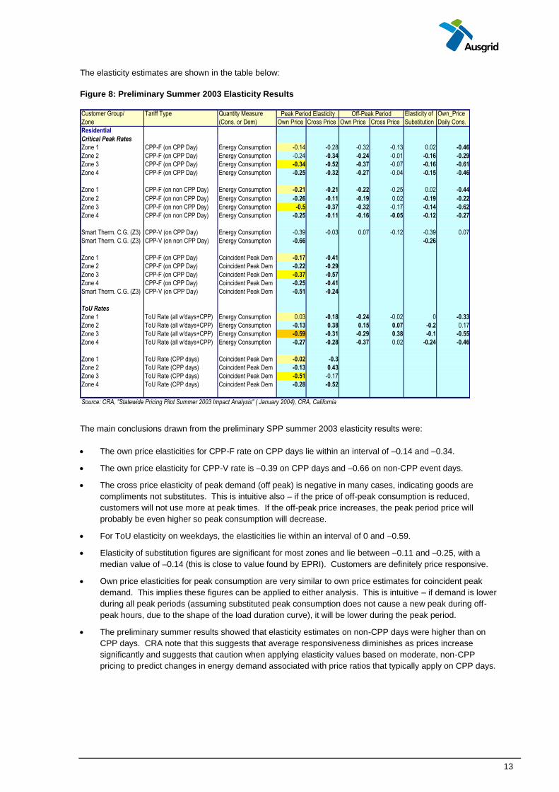
The elasticity estimates are shown in the table below:

Figure 8: Preliminary Summer 2003 Elasticity Results

The main conclusions drawn from the preliminary SPP summer 2003 elasticity results were:

The own price elasticities for CPP-F rate on CPP days lie within an interval of –0.14 and –0.34.

The own price elasticity for CPP-V rate is –0.39 on CPP days and –0.66 on non-CPP event days.

The cross price elasticity of peak demand (off peak) is negative in many cases, indicating goods are

compliments not substitutes. This is intuitive also – if the price of off-peak consumption is reduced,

customers will not use more at peak times. If the off-peak price increases, the peak period price will

probably be even higher so peak consumption will decrease.

For ToU elasticity on weekdays, the elasticities lie within an interval of 0 and –0.59.

Elasticity of substitution figures are significant for most zones and lie between –0.11 and –0.25, with a

median value of –0.14 (this is close to value found by EPRI). Customers are definitely price responsive.

Own price elasticities for peak consumption are very similar to own price estimates for coincident peak

demand. This implies these figures can be applied to either analysis. This is intuitive – if demand is lower

during all peak periods (assuming substituted peak consumption does not cause a new peak during off-

peak hours, due to the shape of the load duration curve), it will be lower during the peak period.

The preliminary summer results showed that elasticity estimates on non-CPP days were higher than on

CPP days. CRA note that this suggests that average responsiveness diminishes as prices increase

significantly and suggests that caution when applying elasticity values based on moderate, non-CPP

pricing to predict changes in energy demand associated with price ratios that typically apply on CPP days.

Customer Group/ Tariff Type Quantity Measure Elasticity of Own_Price

Zone (Cons. or Dem) Own Price Cross Price Own Price Cross Price Substitution Daily Cons.

Residential

Critical Peak Rates

Zone 1 CPP-F (on CPP Day) Energy Consumption -0.14 -0.28 -0.32 -0.13 0.02 -0.46

Zone 2 CPP-F (on CPP Day) Energy Consumption -0.24 -0.34 -0.24 -0.01 -0.16 -0.29

Zone 3 CPP-F (on CPP Day) Energy Consumption -0.34 -0.52 -0.37 -0.07 -0.16 -0.61

Zone 4 CPP-F (on CPP Day) Energy Consumption -0.25 -0.32 -0.27 -0.04 -0.15 -0.46

Zone 1 CPP-F (on non CPP Day) Energy Consumption -0.21 -0.21 -0.22 -0.25 0.02 -0.44

Zone 2 CPP-F (on non CPP Day) Energy Consumption -0.26 -0.11 -0.19 0.02 -0.19 -0.22

Zone 3 CPP-F (on non CPP Day) Energy Consumption -0.5 -0.37 -0.32 -0.17 -0.14 -0.62

Zone 4 CPP-F (on non CPP Day) Energy Consumption -0.25 -0.11 -0.16 -0.05 -0.12 -0.27

Smart Therm. C.G. (Z3) CPP-V (on CPP Day) Energy Consumption -0.39 -0.03 0.07 -0.12 -0.39 0.07

Smart Therm. C.G. (Z3) CPP-V (on non CPP Day) Energy Consumption -0.66 -0.26

Zone 1 CPP-F (on CPP Day) Coincident Peak Dem -0.17 -0.41

Zone 2 CPP-F (on CPP Day) Coincident Peak Dem -0.22 -0.29

Zone 3 CPP-F (on CPP Day) Coincident Peak Dem -0.37 -0.57

Zone 4 CPP-F (on CPP Day) Coincident Peak Dem -0.25 -0.41

Smart Therm. C.G. (Z3) CPP-V (on CPP Day) Coincident Peak Dem -0.51 -0.24

ToU Rates

Zone 1 ToU Rate (all w'days+CPP) Energy Consumption 0.03 -0.18 -0.24 -0.02 0 -0.33

Zone 2 ToU Rate (all w'days+CPP) Energy Consumption -0.13 0.38 0.15 0.07 -0.2 0.17

Zone 3 ToU Rate (all w'days+CPP) Energy Consumption -0.59 -0.31 -0.29 0.38 -0.1 -0.55

Zone 4 ToU Rate (all w'days+CPP) Energy Consumption -0.27 -0.28 -0.37 0.02 -0.24 -0.46

Zone 1 ToU Rate (CPP days) Coincident Peak Dem -0.02 -0.3

Zone 2 ToU Rate (CPP days) Coincident Peak Dem -0.13 0.43

Zone 3 ToU Rate (CPP days) Coincident Peak Dem -0.51 -0.17

Zone 4 ToU Rate (CPP days) Coincident Peak Dem -0.28 -0.52

Source: CRA, "Statewide Pricing Pilot Summer 2003 Impact Analysis" ( January 2004), CRA, California

Peak Period Elasticity Off-Peak Period

14

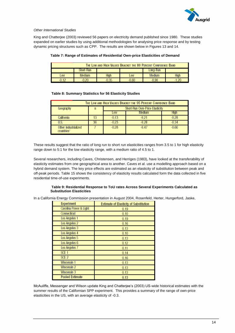
Other International Studies

King and Chatterjee (2003) reviewed 56 papers on electricity demand published since 1980. These studies

expanded on earlier studies by using additional methodologies for analysing price response and by testing

dynamic pricing structures such as CPP. The results are shown below in Figures 13 and 14.

Table 7: Range of Estimates of Residential Own-price Elasticities of Demand

Table 8: Summary Statistics for 56 Elasticity Studies

These results suggest that the ratio of long run to short run elasticities ranges from 3.5 to 1 for high elasticity

range down to 5:1 for the low elasticity range, with a medium ratio of 4.5 to 1.

Several researchers, including Caves, Christensen, and Herriges (1983), have looked at the transferability of

elasticity estimates from one geographical area to another. Caves et al. use a modelling approach based on a

hybrid demand system. The key price effects are estimated as an elasticity of substitution between peak and

off-peak periods. Table 15 shows the consistency of elasticity results calculated form the data collected in five

residential time-of-use experiments.

Table 9: Residential Response to ToU rates Across Several Experiments Calculated as Substitution Elasticities

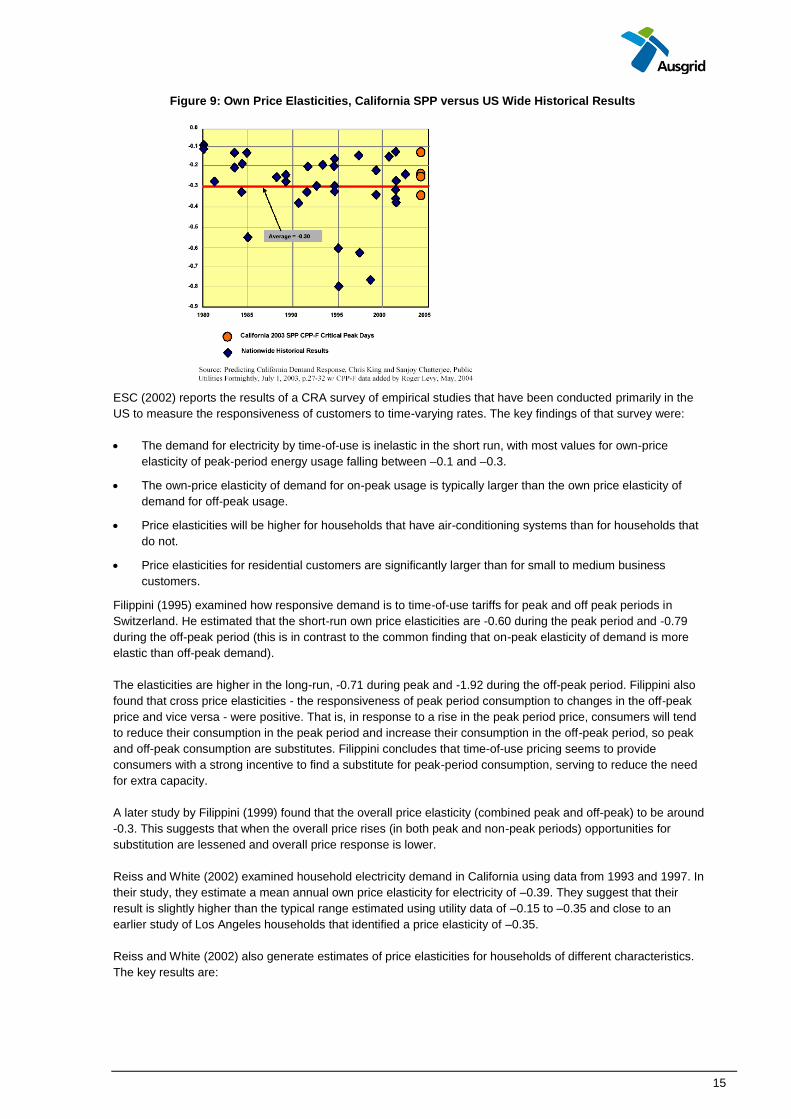
In a California Energy Commission presentation in August 2004, Rosenfeld, Herter, Hungerford, Jaske,

McAuliffe, Messenger and Wilson update King and Chatterjee’s (2003) US-wide historical estimates with the

summer results of the Californian SPP experiment. This provides a summary of the range of own-price

elasticities in the US, with an average elasticity of -0.3.

15

Figure 9: Own Price Elasticities, California SPP versus US Wide Historical Results

ESC (2002) reports the results of a CRA survey of empirical studies that have been conducted primarily in the

US to measure the responsiveness of customers to time-varying rates. The key findings of that survey were:

The demand for electricity by time-of-use is inelastic in the short run, with most values for own-price

elasticity of peak-period energy usage falling between –0.1 and –0.3.

The own-price elasticity of demand for on-peak usage is typically larger than the own price elasticity of

demand for off-peak usage.

Price elasticities will be higher for households that have air-conditioning systems than for households that

do not.

Price elasticities for residential customers are significantly larger than for small to medium business

customers.

Filippini (1995) examined how responsive demand is to time-of-use tariffs for peak and off peak periods in

Switzerland. He estimated that the short-run own price elasticities are -0.60 during the peak period and -0.79

during the off-peak period (this is in contrast to the common finding that on-peak elasticity of demand is more

elastic than off-peak demand).

The elasticities are higher in the long-run, -0.71 during peak and -1.92 during the off-peak period. Filippini also

found that cross price elasticities - the responsiveness of peak period consumption to changes in the off-peak

price and vice versa - were positive. That is, in response to a rise in the peak period price, consumers will tend

to reduce their consumption in the peak period and increase their consumption in the off-peak period, so peak

and off-peak consumption are substitutes. Filippini concludes that time-of-use pricing seems to provide

consumers with a strong incentive to find a substitute for peak-period consumption, serving to reduce the need

for extra capacity.

A later study by Filippini (1999) found that the overall price elasticity (combined peak and off-peak) to be around

-0.3. This suggests that when the overall price rises (in both peak and non-peak periods) opportunities for

substitution are lessened and overall price response is lower.

Reiss and White (2002) examined household electricity demand in California using data from 1993 and 1997. In

their study, they estimate a mean annual own price elasticity for electricity of –0.39. They suggest that their

result is slightly higher than the typical range estimated using utility data of –0.15 to –0.35 and close to an

earlier study of Los Angeles households that identified a price elasticity of –0.35.

Reiss and White (2002) also generate estimates of price elasticities for households of different characteristics.

The key results are:

16

Households with electric space heating or air conditioning exhibit higher price elasticities (-1.0 for space

heating and –0.6 air conditioning) than households without such systems (close to zero for households

without either of these systems);

Lower income households tend to be more sensitive to energy prices than households with medium to

high incomes; and

Elasticities are lower for households that use high amounts of electricity (the authors recognise that this is

a slightly unusual result in light of the two previous conclusions and suggest that it reflects both a weak

correlation between household income and ownership of space heating/air conditioning and the fact that

households tend to substitute toward more price-inelastic electricity use as income rises).

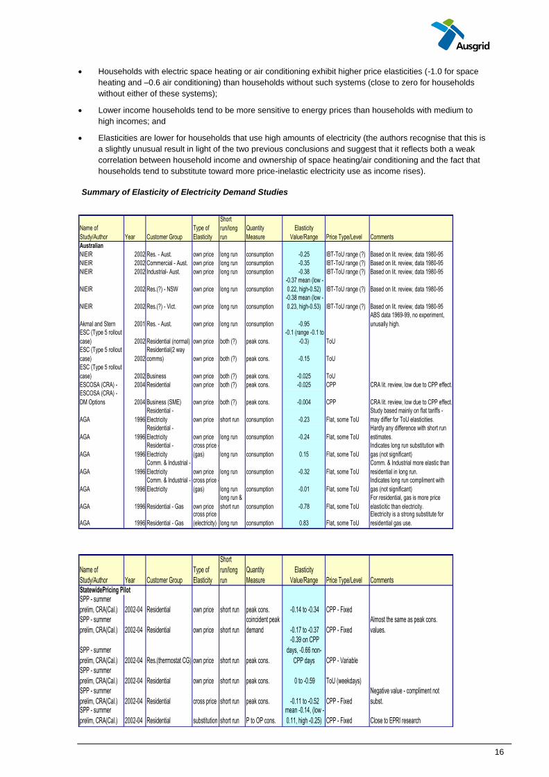
Summary of Elasticity of Electricity Demand Studies

Name of

Study/Author Year Customer Group

Type of

Elasticity

Short

run/long

run

Quantity

Measure

Elasticity

Value/Range Price Type/Level Comments

Australian

NIEIR 2002 Res. - Aust. own price long run consumption -0.25 IBT-ToU range (?) Based on lit. review, data 1980-95

NIEIR 2002 Commercial - Aust. own price long run consumption -0.35 IBT-ToU range (?) Based on lit. review, data 1980-95

NIEIR 2002 Industrial- Aust. own price long run consumption -0.38 IBT-ToU range (?) Based on lit. review, data 1980-95

NIEIR 2002 Res.(?) - NSW own price long run consumption

-0.37 mean (low -

0.22, high-0.52) IBT-ToU range (?) Based on lit. review, data 1980-95

NIEIR 2002 Res.(?) - Vict. own price long run consumption

-0.38 mean (low -

0.23, high-0.53) IBT-ToU range (?) Based on lit. review, data 1980-95

Akmal and Stern 2001 Res. - Aust. own price long run consumption -0.95

ABS data 1969-99, no experiment,

unusally high.

ESC (Type 5 rollout

case) 2002 Residential (normal) own price both (?) peak cons.

-0.1 (range -0.1 to

-0.3) ToU

ESC (Type 5 rollout

case) 2002

Residential(2 way

comms) own price both (?) peak cons. -0.15 ToU

ESC (Type 5 rollout

case) 2002 Business own price both (?) peak cons. -0.025 ToU

ESCOSA (CRA) - 2004 Residential own price both (?) peak cons. -0.025 CPP CRA lit. review, low due to CPP effect.

ESCOSA (CRA) -

DM Options 2004 Business (SME) own price both (?) peak cons. -0.004 CPP CRA lit. review, low due to CPP effect.

AGA 1996

Residential -

Electricity own price short run consumption -0.23 Flat, some ToU

Study based mainly on flat tariffs -

may differ for ToU elasticities.

AGA 1996

Residential -

Electricity own price long run consumption -0.24 Flat, some ToU

Hardly any difference with short run

estimates.

AGA 1996

Residential -

Electricity

cross price -

(gas) long run consumption 0.15 Flat, some ToU

Indicates long run substitution with

gas (not significant)

AGA 1996

Comm. & Industrial -

Electricity own price long run consumption -0.32 Flat, some ToU

Comm. & Industrial more elastic than

residential in long run.

AGA 1996

Comm. & Industrial -

Electricity

cross price -

(gas) long run consumption -0.01 Flat, some ToU

Indicates long run compliment with

gas (not significant)

AGA 1996 Residential - Gas own price

long run &

short run consumption -0.78 Flat, some ToU

For residential, gas is more price

elasticitic than electricity.

AGA 1996 Residential - Gas

cross price

(electricity) long run consumption 0.83 Flat, some ToU

Electricity is a strong substitute for

residential gas use.

Name of

Study/Author Year Customer Group

Type of

Elasticity

Short

run/long

run

Quantity

Measure

Elasticity

Value/Range Price Type/Level Comments

StatewidePricing PilotSPP - summer

prelim, CRA(Cal.) 2002-04 Residential own price short run peak cons. -0.14 to -0.34 CPP - Fixed

SPP - summer

prelim, CRA(Cal.) 2002-04 Residential own price short run

coincident peak

demand -0.17 to -0.37 CPP - Fixed

Almost the same as peak cons.

values.

SPP - summer

prelim, CRA(Cal.) 2002-04 Res.(thermostat CG) own price short run peak cons.

-0.39 on CPP

days, -0.66 non-

CPP days CPP - Variable

SPP - summer

prelim, CRA(Cal.) 2002-04 Residential own price short run peak cons. 0 to -0.59 ToU (weekdays)

SPP - summer

prelim, CRA(Cal.) 2002-04 Residential cross price short run peak cons. -0.11 to -0.52 CPP - Fixed

Negative value - compliment not

subst.SPP - summer

prelim, CRA(Cal.) 2002-04 Residential substitution short run P to OP cons.

mean -0.14, (low -

0.11, high -0.25) CPP - Fixed Close to EPRI research

17

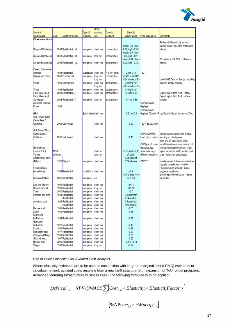
Use of Price Elasticities for Avoided Cost Analysis

Where elasticity estimates are to be used in conjunction with long run marginal cost (LRMC) estimates to

calculate network avoided costs resulting from a new tariff structure (e.g. expansion of ToU rollout programs,

Advanced Metering Infrastructure business case), the following formulae is to be applied:

n

t

jtkjkj FactorElasticityElasticityCostWACCNPVDeferral1

,, @

Name of

Study/Author Year Customer Group

Type of

Elasticity

Short

run/long

run

Quantity

Measure

Elasticity

Value/Range Price Type/Level Comments

Other International

King and Chatterjee 2003 Residential - all own price short run consumption

mean -0.2, (low -

0.12, high -0.35)

Reviewed 56 electricity demand

studies since 1980, 80% confidence

interval.

King and Chatterjee 2003 Residential - all own price long run consumption

mean -0.9, (low -

0.6, high -1.2)

King and Chatterjee 2003 Residential - US own price short run consumption

mean -0.28, (low -

0.23, high -0.34)

36 studies in US, 95% confidence

interval.

Caves, Christensen,

Herriges 1983 Residential substitution short run P to OP cons. 0.1 to 0.19 ToU

Sayers and Shield 2001 Commercial own price long run consumption -0.435 to -0.8313

Wade 1999 Commercial own price

long and

short run consumption

-0.24 short run & -

0.25 long run

Used in US Dept. of Energy modelling

study of energy industry

Wade 1999 Residential own price

long and

short run consumption

-0.23 short run & -

0.31 long run

Fatai, Oxley and 2003 Residential (?) own price short run consumption -0.18 to -0.24 Expect higher than Aust., >space

Fatai, Oxley and

Scrimgeour 2003 Residential (?) own price long run consumption -0.44 to -0.59

Expect higher than Aust., >space

heating.

American Electric

Power 1992

CPP (in-house

display)

GPU Substitution short run -0.31 to -0.4

CPP (in-house

display), 50c/kWh P significantly higher than normal ToU

Gulf Power "Good

Cents Select",

California 2002 Gulf Power short run -0.37 ToU P $0.093/kWh

Gulf Power "Good

Cents Select",

California 2002 Gulf Power short run -0.11

CPP $0.29 kWh,

load control device

high customer satisfaction, limited

warning of critical peaks

Electricite de

France (EdF)

Tempo

1996

onwards

short to

long run

-0.79 peak, -0.18

off-peak.

CPP type - 2 intra-

day rates, red,

white, blue days,

different expenses

peak and off-peak found to be

substitutes (ie no conservation), but

cross price elasticites small, much

higher rates than in US studies, trial

rates higher than actual rates

Swiss Households

(Fillipini) 1995 Filippini own price short run

-0.6 peak and -

0.79 off peak CPP ?? results appear to be counter-intuitive

Fillipini (Swiss

households) 1999 Residential substitution short run -0.3

suggets compliements - earlier

Filippini studies showed + subst.,

suggests substitutes.

Reiss and White 2002 Residential own price all

-0.39 (range -0.15

to -0.35)

Electric space heating, a/c - higher

elasticities.

Nan and Murray 1991 Residential own price short run -0.611

Beenstock et al. 1999 Residential own price long run -0.579

Tiwari 2000 Residential own price short run -0.7

Herriges and King 1994 Residential own price short run -0.2 (summer)

Residential own price short run -0.4 (winter)

Archibald et al. 1982 Residential own price short run -0.4 (summer)

Residential own price short run -0.48 (winter)

Barnes et al. 1981 Residential own price short run -0.55

Dubin 1985 Residential own price short run -0.16

Dubin and

McFadden 1984 Residential own price short run -0.25

Goett and

McFadden 1982 Residential own price short run -0.17

Houston 1982 Residential own price short run -0.28

McFadden et al. 1977 Residential own price short run -0.37

Chang and Hsing 1991 Residential own price short run -0.33

Silk and Joutz 1997 Residential own price short run -0.62

Bjorner et al. 2002 Residential own price short run -0.4 to -0.13

Vaaga 1993 Residential own price long run -0.27

kjkj Energyice ,, %Pr%

18

Where:

Deferralj,k = avoided network costs (capital and operating expenditure) in ToU period j (i.e. peak, shoulder or off-

peak) for pricing structure k (i.e. ToU, CPP);

WACC = Discount rate, which is the Weighted Average Cost of Capital from Network Determination;

n = number of years in the marginal cost study (typically 10-15);

Costj,k = network LRMC allocated to ToU period j under tariff k using method of intercepts analysis and

%Energyj,k;

Elasticityt = own price elasticity of electricity consumption estimate for year t;

ElasticityFactorj = elasticity scale factor based on time period – 1 for peak, 0.8 for shoulder and off-peak;

%Pricej,k = percentage price change at ToU period j under tariff k compared to existing tariff; and

%Energyj,k = proportion of total energy usage at ToU period j under tariff k.

When LRMC is applied in this manner, the elasticity estimates are applied cumulatively, not on an incremental basis.

(viii) Key conclusions and recommendations

Based on domestic and international studies, the common range for short run estimates of the own price

elasticity of electricity (peak consumption) is –0.1 to –0.3. Estimates may be as low as –0.025 and as high

as –0.6.

Long run estimates of the own price elasticity of residential demand exceed the short run measures, as

consumers purchase more energy efficient appliance stock. The long run value can be around –0.6,

although some studies have placed this value above 1.

There are less studies available on the own price elasticities of commercial and industrial customers. In

the short run, some have suggested a very inelastic response (in the order of –0.005). However, in the

long run, some studies suggest that the elasticity value can exceed the residential estimates (-0.35 to –

0.8). More information on this sector would be useful.

Although even the typical higher end of these estimates (e.g. -0.3 range) is still considered to be relatively

inelastic in economic terms, it is sufficient to defer enough demand to save a substantial amount in

avoided costs (especially when all upstream and downstream benefits are factored into the analysis).

Hence a planned network project can still yield a positive NPV value on the back of a relatively inelastic

price response.

The results of studies by CRA suggest that although the elasticity increases with higher price levels, the

elasticity value can actually decrease at high CPP prices, as there are diminishing returns as discretionary

load is limited.

The summer 2003 SPP results suggest that own price elasticities for peak consumption are practically the

same as own price elasticities based on peak demand. This implies elasticity figures can be applied to

either analysis. This is intuitive – if demand is lower during all peak periods (assuming substituted peak

consumption does not cause a new peak during off-peak hours, due to the shape of the load duration

curve), it will be lower during the peak period.

The substitution effect associated with peak price rises dominates the conservation effect (positive cross

price elasticities of off-peak consumption with peak price).

Elasticities in warmer climates can be as much as double those in cooler climates.

High air conditioning penetration rates drive higher elasticities.

Although the provision of information can affect elasticity response, price signals are necessary in order to

produce sustainable load reductions.

19

Bibliography of Relevant Studies

Acton, Jan Paul and Bridger M. Mitchell, “Evaluating time-of-day electricity rates for residential customers,” in

Bridger M. Mitchell and Paul R. Kleindorfer (editors), Regulated industries and public enterprise: European and

United States perspectives (Lexington Books, Lexington, MA),1980.

Aigner, Dennis J. (editor). “Welfare Econometrics of Peak-load Pricing For Electricity,” Journal of Econometrics,

Annals 3, 26, 1984.

Aigner, D. J. and J. G. Hirschberg, “Commercial/industrial customer response to time-of-use electricity prices:

some experimental results,” Rand Journal of Economics, Vol. 16, No. 3,341-355, Autumn 1985.

Aigner, D. J., J. Newman and A. Tishler, “The Response of Small and Medium-Size Business Customers to

Time-of-Use (TOU) Electricity Rates in Israel,” Journal of Applied Econometrics, Vol. 9, 283-304, 1994.

Akmal, M. and Stern, D., “The Structure of Australian Residential Energy Demand, ANU Working Papers in

Ecological Economics”, Number 0101, March 2001.

American Electric Power, “Report on the Variable Energy Pricing and TransText Advanced Energy Management

Pilot,” Columbus, Ohio, 1992.

Archibald, R.B., Finifter, D.H. and Moody, C.E. 1982, ’Seasonal Variation in Residential Electricity Demand:

Evidence for Survey Data’, Applied Economics, vol. 14, pp 167–81.

Aubin, Christophe, Denis Fougere, Emmanuel Husson and Marc Ivaldi, “Real-time pricing of electricity for

residential customers: econometric analysis of an experiment,” Journal of Applied Econometrics 10 1995, S171-

191.

Australian Gas Association (1996), “Price Elasticities of Australian Energy Demand”, AGA Research paper No.

3, AGA, Canberra.

Braithwait, Steven, “Residential TOU Price Response in the Presence of Interactive Communication

Equipment,” in Ahmad Faruqui and Kelly Eakin, editors, Pricing in Competitive Electricity Markets, Kluwer

Academic Publishing, 2000, pp. 359-373.

Caves, Douglas W. and Laurits R. Christensen, “Econometric Analysis of Residential Time-of-Use Electricity,”

Journal of Econometrics, 1980.

Caves, Douglas W., Laurits R. Christensen and Joseph A. Herriges, “Consistency of Residential Customer

Response in Time-of-Use Pricing Experiments, Journal of Econometrics, 1984, 26, pp.179-203.

Caves, Douglas W., Joe Herriges and K. Kuester, “Load shifting under voluntary residential time-of-use rates,”

The Energy Journal 10 1989, pp. 83-99.

Faruqui, Ahmad, Dennis J. Aigner and Robert T. Howard, Customer Response to Time-of-Use Rates: Topic

Paper 1, EPRI EURDS Report Number 84, March 1981.

Faruqui, Ahmad and J. Robert Malko, “The Residential Demand for Electricity by Time-of-Use: A Survey of

Twelve Experiments with Peak Load Pricing,” Energy 8 (10) 1983, pp. 781-795.

Faruqui, Ahmad, Susan S. Shaffer, Kenneth P. Seiden, Susan Blanc and John H. Chamberlin, Customer

Response to Rate Options, EPRI Report Number CU-7131, January 1991.

Faruqui, Ahmad, Hung-po Chao, Victor Niemeyer, Jeremy Platt and Karl Stahlkopf, “Analyzing California’s

Power Crisis,” The Energy Journal, Vol. 22, No. 4, 2001.

Filippini, Massimo, “Swiss Residential Demand for Electricity by Time-of-Use: An Application of the Almost Ideal

Demand System,” The Energy Journal, 16 (1), 1995, pp. 27-39.

Filippini, Massimo, “Swiss residential demand for electricity by time-of-use,” Resource and Energy Economics,

17 (3), November 1995, pp. 281-290.

Giraud, Denise and Christophe Aubin, “Tempo: A new real-time tariff for residential customers,” in Proceedings:

1994 Innovative Electricity Pricing Conference, EPRI TR-103629, February 1994.

Goett, Andrew A., “Can residential time-of-use rates work? The recent experience,” in Proceedings: 1994

Innovative Electricity Pricing Conference, EPRI TR-103629, February 1994.

20

Hendricks, W., R. Koenker and D. J. Poirier, “Residential Demand for Electricity by Time-of-Day: An

Econometric Approach,” Electric Power Research Institute, EA-704 (1978).

Hill, D. H., et al, “Evaluation of the FEA’s Load Management and Rate Design Demonstration Projects,” Electric

Power Research Institute, EA-1152 (1979).

Kirkeide, Loren, “Reducing Power Capacity Requirements Using Two-Period Time-of-Use Rates with Ten-Hour

Peak Periods,” Master’s Thesis, Arizona State University, 1989.

Lawrence, Anthony G. and Dennis J. Aigner (editors), “Modeling and forecasting time-of-day and seasonal

electricity demands,” Journal of Econometrics, Annals 1, 9, 1979.

Lifson, D., “Comparison of Time-of-use Electricity Demand Models,” Research Triangle Institute, Doc. No. 133,

(March, 1981).

Miedema, A. K., et al. “Time-of-Use Electricity Price Effects: Summary I,” Research Triangle Institute, Report

(June, 1980).

Mitchell, B. M. and J. P. Acton, “Electricity Consumption by Time-of-Use in a Hybrid Demand System,” Rand

Corporation Rep. R-2628-DWP/HF, (Dec. 1980)

Parks, R. W. and David Weitzel, “Measuring the customer welfare effects of time-differentiated electricity

prices,” Journal of Econometrics, Annals 3, 26, 35-64.

Puget Sound Energy, “Advice No. 2001-36: Electric Tariff Filing,” Submitted to the Washington Utilities and

Transportation Commission, August 31, 2001.

Woo, C K., “Demand for electricity of small non-residential customers under Time-of-Use (TOU) Pricing,” The

Energy Journal, Vol. 6, No. 4, 115-127, 1985.

Additional

“Flavors of Elasticity of Demand: A Reference,” p. 32). How do customers react to hourly prices?

Rosenfeld, A., Herter, K., Hungerford, D., Jaske, M., McAuliffe, P., Messenger M., and Wilson, J., Demand

Response Hardware and Tariffs: California’s Vision and Reality, August 2004, ACEE Summer Study, California

Energy Commission.

King, C., and Chatterjee, S., “Predicting California Demand Response” , Public Utilities Fortnightly, July 1, 2003,

pp. 27-32.

Faruqui, A., and George, S. S.,(year unknown), Dynamic pricing Revisited: California Experiments in Mass

Market, Paper presented at Eastern Conference in Providence, Rhode Island.

California Energy Commission (2004), Statewide Pricing Pilot (SPP), Overview and Design Features,

presentation.

Essential Services Commission (2002), “Installing Interval meters for Electricity Customers – Costs and

benefits: Position Paper, Melbourne.

Charles River Associates (2004), “Assessment of Demand Management and Metering Strategy Options”,

Submitted to Essential Services Commission of South Australia (ESCOSA), Melbourne.

Intelligent Energy Services (1999), “Evaluation of Metering Strategies for Full Retail Contestability”, A Project

Commissioned by the Victorian Full Retail Contestability Co-Ordination Committee, Melbourne.

Charles River Associates (2004), “Statewide Pricing Pilot: Summer 2003 Impact Analysis”, Draft Report,

California.

Langmore, M., and Dufy, G., (2004) “Domestic Electricity Demand Elasticities: Issues for the Victorian Energy

Market”, Consumer Utilities Advocacy Centre,

IPART, “Inclining Block Tariffs for Electricity Network Services”, Secretariat Discussion Paper, June 2003,

IPART, Sydney.

National Institute of Economic and Industry Research, “The Price Elasticity of Demand for Electricity in NEM

regions”, prepared for National Electricity Market Management Company, June 2002.

21

Barne, R., Gillingham, R. and Hagemann, R. 1981, ‘The Short-Run Residential Demand for Electricity’, The

Review of Economics and Statistics, vol. 62, pp 541-51.

Beenstock, M., Goldin, E. and Nabot, D. 1999, ‘The demand for electricity in Israel’, Energy Economics, vol. 21,

no. 2, pp 168–83.

Bjorner, T. and H. Jensen, 2002, 'Interfuel substitution within Industrial Companies: an analysis based upon

panel data at company level’, The Energy Journal, Vol 23, No. 2, pp 27-50.

Chang, H.S. and Hsing, Y. 1991, ‘The demand for residential electricity: new evidence on time varying

elasticities’, Applied Economics, vol. 23, pp 1251–6.

Dubin, J.A. 1985, ‘Evidence of Block Switching in Demand Subject in Declining Block Rates — A New

Approach’, Social Science Working Paper, no. 583, California Institute of Technology, Department of

Economics.

—— and McFadden, D.L. 1984, ‘An Econometric Analysis of Residential Appliance Holdings and Consumption’,

Econometrica, vol. 52, pp 345–62.

ESC [Essential Services Commission of Victoria] 2002, ‘Installing interval meters for electricity customers —

costs and benefits — position paper’, November, ESC Victoria.

Fatai, K., Oxley, L., and F. Scrimgeour, 2003. 'Modeling and forecasting the demand for electricity in New

Zealand: A comparison of alternative approaches', The Energy Journal, Vol 24, No.1.

Filippini, M, 1995. 'Swiss residential demand for electricity by time-of-use', Resource and Energy Economics,

17, pp 281-290.

Filippini, M, 1999. 'Swiss residential demand for electricity', Applied Economic Letters, 6, pp 533-538.

Filippini, M. and Pachauri, S. 2002, ‘Elasticities of electricity demand in urban Indian households'’ CEPE

Working Paper No. 16, Centre for Energy Policy and Economics, Zurich, Switzerland.

Goett, A. and McFadden, D.L. 1982, ‘Residential End-Use Energy Planning System (REEPS)’, Electric Power

Institute, EA-2512, Final Report, July.

Herriges, J.A. and King, K.K. 1994, ‘Residential Demand for Electricity Under Inverted Block Rates: Evidence

from a Controlled Experiment’, Journal of Business and Economic Statistics, vol. 12, no. 4, pp 419–30.

Houston, D.A. 1982, ‘Revenue Effects from Changes in a Declining Block Structure’, Land Economics, vol. 58,

pp 336–51.

McFadden, D.A., Puig, C. and Kirshner, D. 1977, ‘Determinants of the Long-Run Demand for Electricity, in

Proceedings of the Business and Economic Statistics Section, American Statistical Association, pp 109–19.

Miller, J 2001, ‘Modelling residential demand for electricity in the U.S: a semiparametric panel data approach’,

Unpublished draft manuscript, Rice University. Nan, G.D. and Murry, D.A., 1991, ‘Energy Demand with the

Flexible Double-Logarithmic Functional Form’, The Energy Journal, vol. 13, no. 4, pp 149–59.

NIEIR 2002, ‘The price elasticity of demand for electricity in NEM regions’, Report prepared for NEMMCO, June,

Victoria.

Reiss, P. and White, M. 2002, ’Household electricity demand, revisited’. Unpublished manuscript, Graduate

School of Business, Stanford University, http://www.stanford.edu/~mwwhite/demand.pdf.

Silk, J.I. and Joutz, F.L., 1997, ‘Short and long-run elasticities in US residential electricity demand: a

cointegration approach’, Energy Economics, vol. 19, no. 4, pp 493–513.

Sayers, C and Shield, D. 2001, Electricity Prices and Cost Factors, Staff Research Paper, Productivity

Commission, Canberra.

Tiwari, P., 2000, ‘Architectural, Demographic and Economic Causes of Electricity Consumption in Bombay’,

Journal of Policy Modelling, vol. 22, no. 1, pp 81–98.

Vaage, K. 1993, 'The dynamics of residential electricity demand: empirical evidence from Norway',Working

Paper No. 0193, Department of Economics, University of Bergen, Norway.

Wade, S 1999. Price Responsiveness in the NEMS Buildings Sector Model, Report No. EIA/DOE- 0607(99),

http://www.eia.doe.gov/oiaf/issues/building_sector.html.