Appendix E: The Upper Rio Grande Simulation Model … · 17 Riparian ET between San Acacia and...
149
U.S. Department of the Interior Bureau of Reclamation Upper Colorado Region Albuquerque Area Office December 2013 Appendix E: The Upper Rio Grande Simulation Model (URGSiM)
Transcript of Appendix E: The Upper Rio Grande Simulation Model … · 17 Riparian ET between San Acacia and...

U.S. Department of the Interior Bureau of Reclamation Upper Colorado Region Albuquerque Area Office December 2013
Appendix E: The Upper Rio Grande Simulation Model (URGSiM)

Mission Statements The U.S. Department of the Interior protects America’s natural resources and heritage, honors our cultures and tribal communities, and supplies the energy to power our future. The mission of the Bureau of Reclamation is to manage, develop, and protect water and related resources in an environmentally and economically sound manner in the interest of the American public. Sandia Laboratory Climate Security program works to understand and prepare the nation for the national security implications of climate change. The U.S. Army Corps of Engineers Mission is to deliver vital public and military engineering services; partnering in peace and war to strengthen our Nation’s security, energize the economy and reduce risks from disasters.

Acronyms and Abbreviations
ABCWUA Albuquerque Bernalillo County Water Utility Authority
amsl above mean sea level
ASCE American Society of Civil Engineers
BIA Bureau of Indian Affairs
CDWR Colorado Department of Water Resources
cfs cubic feet per second
dd decimal degree
EBID Elephant Butte Irrigation District
ET evapotranspiration
LFCC Low Flow Conveyance Channel
MRGWA Middle Rio Grande Water Assessment
REDW Reclamation Emergency Drought Water
SS Steady state
SB South boundary
TR-21 Technical Release No. 21 (United States Department of Agriculture 1970)
URGIA Upper Rio Grande Impact Assessment
URGSiM Upper Rio Grande Simulation Model
URGWOM Upper Rio Grande Water Operation Model
USGS U.S. Geological Survey


Reclamation, USACE, and E-i Sandia National Laboratories
Table of Contents Page
I. URGSiM Extent, Resolution, and Data Requirements......................... E-1 I.A. Spatial Extent, Resolution, and Data Requirements ...................... E-1
I.A.1. Surface Water ............................................................... E-1 I.A.2. Groundwater ................................................................. E-3 I.A.3. Cities ............................................................................ E-3
I.B. URGSiM Temporal Extent, Resolution, and Data Requirements ............................................................................ E-6
II. URGSiM Mass Balance Calculations .................................................... E-8
II.A. Groundwater Mass Balance .......................................................... E-8 II.A.1. Groundwater Discharge above Chamita
and Embudo ............................................................... E-8 II.A.2. Dynamic Regional Groundwater Modeling ................. E-12
II.B. Surface Water Mass Balance ...................................................... E-32 II.B.1. River Reach Mass Balance .......................................... E-34 II.B.2. Agricultural Conveyance Mass Balance ...................... E-39 II.B.3. Reservoir Mass Balance .............................................. E-39
III. Evapotranspiration Calculations in URGSiM .................................... E-44
III.A. Reference Evapotranspiration (ET) Equations ............................ E-45 III.A.1. Modified Penman ETo Problems ................................. E-46 III.A.2. Choosing a New ETo Calculation ................................ E-46
III.B. Crop Coefficients ....................................................................... E-51 III.B.1. Issues with the Sammis et al. (1985) Crop
Coefficients .............................................................. E-52 III.B.2. Current Crop Coefficient Methods .............................. E-56
III.C. Vegetation Classifications .......................................................... E-66 III.C.1. Irrigated Agriculture ................................................... E-66 III.C.2. Riparian Vegetation .................................................... E-67
III.D. Effective Precipitation ................................................................ E-69 III.E. Implications of Changed Methods on Historic Mass Balance ...... E-70 III.F. Reservoir Operations in URGSiM .............................................. E-72
III.F.1. Overall Water Operations ............................................ E-73 III.F.2. Heron Reservoir Operations ........................................ E-73 III.F.3. El Vado Reservoir Operations ..................................... E-74 III.F.4. Abiquiu Reservoir Operations ..................................... E-78 III.F.5. Cochiti Reservoir Operations ...................................... E-78 III.F.6. Jemez Reservoir Operations ........................................ E-78 III.F.7. Elephant Butte Reservoir Operations ........................... E-79 III.F.8. Caballo Reservoir Release Rules ................................. E-79
III.G. URGSiM Calibration, Validation and Implications on Uncertainty .............................................................................. E-80

E-ii Reclamation, USACE, and
Sandia National Laboratories
III.G.1. Observation Uncertainties ........................................... E-81 III.G.2. Calibration Residuals .................................................. E-86 III.G.3. Validation Residual Analysis for Stream Flow
Observations ............................................................... E-97 III.G.4. Validation Residual Analysis for Reservoir Storage
Observations ..............................................................E-102 III.H. URGSiM Reach Specific Information and Descriptions .............E-106
III.H.1. San Juan-Chama Diversions to Azotea Tunnel Outlet ......................................................................E-106
III.H.2. Compact Index Gages to Lobatos ...............................E-108 III.J. Additional Groundwater Data and Results .................................E-115
IV. Bibliography ....................................................................................... E-130 Tables Table Page 1 Reservoirs Simulated in URGSiM .................................................. E-1 2 URGSiM Input Gages .................................................................... E-4 3 URGSiM Calibration Gages ........................................................... E-5 4 Climate Stations Used for Climate Inputs to URGSiM. .................. E-6 5 Constant Groundwater Contribution Added to Reaches above
Rio Grande Rio Chama Confluence ........................................... E-11 6 Specified Fluxes (T) to the 16-Zone Spatially Aggregated
Espanola Basin Groundwater Model .......................................... E-16 7 Darcy-Based Calculations to Estimate Steady State Flow in
North-South Direction for Socorro Groundwater Basin Shallow and Central Regional Aquifer Zones ............................ E-23
8 Estimated Steady StateGroundwater Flows Between Socorro Groundwater Basin Zones, and to the South Boundary for the 12-Zone Spatially Aggregated Model................................... E-24
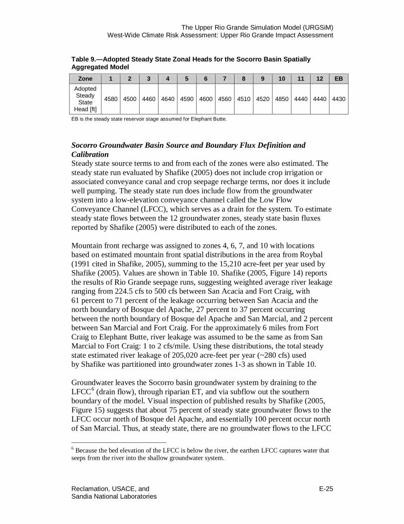
9 Adopted Steady State Zonal Heads for the Socorro Basin Spatially Aggregated Model ...................................................... E-25
10 Steady State Fluxes Adopted for 12-Zone Socorro Basin Model ........................................................................................ E-26
11 Percent of Total Flow Past Points South of Cochiti Reservoir that is in Agricultural Conveyance System ................................ E-33
12 Reach Summary Table ................................................................. E-36

Reclamation, USACE, and E-iii Sandia National Laboratories
Tables (continued) Table Page 13 Channel Geometry Relationships Adopted at Selected Gages,
Used to Estimate Stage and Area as a Function of Flow Rate in Reaches above Cochiti Reservoir. .......................................... E-37
14 Open Water Area of Reaches below Cochiti Reservoir as a Function of River Flow.............................................................. E-38
15 Modeled Reservoirs Summary Information .................................. E-40 16 Winter Reservoir Coefficient of Proportionality ( ) for the
Five Upper Reservoirs ............................................................... E-42 17 Reference ET (ETo), Actual ET (Eta) in Non-Weighing
Lysimeters, and Yields in the Lysimeters and Surrounding Field Crop Yields Reported by Sammis et al (1985) for Alfalfa ....................................................................................... E-55
18 Open Water Evaporation (crop) Coefficients Calculated from Temperature and Pan Evaporation Data Measured at Five Reservoirs in New Mexico between 1975 and 2006 ................... E-66
19 Storage Factor (sf) as a Function of Irrigation Application Depth Used to Estimate Monthly Effective Precipitation with the TR-21 Method (United States Department of Agriculture 1970) ...................................................................... E-70
20 Summary of Changes to ET Methods Described in this Document (rows above greyed out row), and Resulting Changes to Total ET and Ungaged Inflows (Model Calibration Term) for URGSiM Reaches Below Cochiti Reservoir .............. E-71
21 Contracted San Juan-Chama Project Water Volumes Used by URGSiM ................................................................................... E-73
22 End of Month Prior And Paramount Storage Targets Currently Used in URGSiM ...................................................................... E-75
23 Irrigation Demand (cfs) at Cochiti Reservoir, Including Prior and Paramount Demands ........................................................... E-77
24 Target Releases Used for Elephant Butte and Caballo Reservoirs to Determine Releases in Validation and Scenario Evaluation Modes (Acre-Feet) .................................................................... E-79
25 Surface Water Calibration Methods and Magnitude of the Calibration Term for URGSiM Reaches and Reservoirs ............ E-82
26 95 Percent Confidence Intervals for Calibration Gages (Table 3).................................................................................... E-84
27 Minimum Flow Requirements below the Three San Juan Basin Diversions into San Juan-Chama Project ..................................E-108
28 Calibration Parameters Related to Groundwater ..........................E-113 29 Calibration Parameters Related to Canal Leakage ........................E-113
mrk ,

E-iv Reclamation, USACE, and
Sandia National Laboratories
Tables (continued) Table Page 30 Calibration Parameters Related to Reservoirs ..............................E-114 31 Calibration Parameters Related to Reaches ..................................E-114 32 Unit Head Flow Matrix (connectivity and head dependent flow
relations) for Zones 1 through 17 of the 51-Zone Albuquerque Basin Compartmental Model (ft2/day) ......................................E-117
33 Unit Head Flow Matrix (connectivity and head dependent flow relations) for Zones 18 through 34 of the 51-Zone Albuquerque Basin Compartmental Model (ft2/day) .................E-119
34 Unit Head Flow Matrix (connectivity and head dependent flow relations) for Zones 35 through 51 of the 51-Zone Albuquerque Basin Compartmental Model (ft2/day) .................E-121
35 Zone Bottom Elevations (ft above mean sea level), Areal Extent (km2), and Initial Heads (feet above mean sea level) for the Spatially Aggregated Albuquerque Basin Groundwater Model .......................................................................................E-123
36 Zone Bottom Elevations (ft msl), Areal Extent (square kilometers), and Initial Heads (feet above mean sea level) for the Spatially Aggregated Espanola Basin Groundwater Model .......................................................................................E-124
37 Unit Head Connectivity Matrix (connectivity and head-dependent flow relations) for 16-Zone Espanola Basin Compartmental Model (ft2/month). ....................................................................E-125
38 Calibration Parameters for Stream-Aquifer Interactions in Spatially Aggregated Espanola Basin Groundwater Model .......E-126
39 Head-Dependent Boundary Flow Parameters for Spatially Aggregated Espanola Basin Groundwater Model ......................E-126
40 Unit Head Flow Matrix (connectivity and head-dependent flow relations) for 12-Zone Socorro Basin for Spatially Aggregated Groundwater Model (acre/month). SB signifies the south boundary, which is assumed to be Elephant Butte Reservoir for all southern zones (3, 10-12). ..............................................E-126
41 URGSiM Surface Water Groundwater Interaction Parameters for Albuquerque and Socorro Groundwater Basins ...................E-127
42 Estimated Groundwater Head Values for January 1975 ...............E-128

Reclamation, USACE, and E-v Sandia National Laboratories
Figures
Figure Page 1 The Upper Rio Grande Basin. URGSiM models do not include
for example, the Rio Salado, or the Rio San Jose, and only includes the Rio Puerco as gaged inflows to the Rio Grande. .......... E-2
2 URGSiM spatial extent including input gages, calibration gages, modeled reservoirs, and groundwater basins ..................... E-7
3 Uncorrected and corrected winter residuals for the Lobatos to Cerro reach 1975 through 1999.............................................. E-11
4 Spatial extent of Frenzel (1995) regional groundwater model of the Espanola Basin. Taken from Frenzel (1995), Figure 1. ..... E-13
5 Spatially aggregated zones used for simulation of Espanola Basin groundwater system. ........................................................ E-14
6 Estimated Santa Fe sewage return values 1975 through 1999........ E-16 7 Well extraction input data for the Espanola Basin 1975
through 1999. ............................................................................ E-17 8 Stream-aquifer interactions for the Rio Grande–Espanola basin
groundwater system north of Otowi gage. .................................. E-18 9 Simulated groundwater flows from the Espanola Basin to the
Albuquerque Basin from 1975 through 1999 ............................. E-19 10 Drawdown in the Espanola Basin from 1975 to 1992 as
modeled by Frenzel (1995) and the 16-zone compartmental groundwater model. ................................................................... E-20
11 Net groundwater movement between Espanola basin groundwater zones. At each timestep, the absolute value of all flows between any two zones is summed as a comparison metric to help evaluate the ability of the 16-zone compartmental model to capture the overall groundwater movement patterns. ... E-20
12 Active model grid for Shafike (2005) groundwater model of Socorro groundwater basin (left), and zone delineation for the spatially aggregated model (right) ................................................ E-21
13 Well pumping assumed for Socorro Basin 1975 through 1999, based on estimates of municipal and industrial use and supplemental irrigation demand. ................................................ E-28
14 Modeled groundwater heads in Socorro Basin by groundwater zone from 1975 through1999 ..................................................... E-29
15 Flows from the groundwater system to the LFCC for Rio Grande reaches from San Acacia to Elephant Butte Reservoir as modeled by the coupled monthly timestep model, the URGWOM surface water model, and steady state values reported by Shafike (2005). .......................................................................... E-29
E-vi Reclamation, USACE, and
Sandia National Laboratories
Figures (continued)
Figure Page 16 Rio Grande river leakage San Acacia to Elephant Butte
Reservoir as modeled by the coupled monthly timestep model, the URGWOM surface water model, and steady state values reported by Shafike (2005). .................................... E-30
17 Riparian ET between San Acacia and Elephant Butte Reservoir as modeled by the coupled monthly timestep model, the URGWOM surface water model, and steady state values reported by Shafike (2005). ....................................................... E-31
18 Crop seepage between San Acacia and Elephant Butte Reservoir as modeled by the coupled monthly timestep model and the URGWOM surface water model. ............................................... E-31
19 Average river and agricultural conveyance flows through the Rio Grande system from 1975 through1999............................... E-33
20 Cumulative Reference ET (ETo) calculated at Angostura weather station during the year 2007 by a variety of ETo equations. ............................................................................ E-47
21 Comparison of monthly calculations of ETo in centimeters per day (cm/da) using the Hargreaves equation (x-axis) to monthly averages of daily calculations of ETo using the same (y-axis) shows an almost imperceptible difference between the two methods for 12 years of Angostura weather station data ...... E-48
22 Weather station data available along river reaches within the URGSiM model extent with periods of record starting before the year 2000. ............................................................................ E-50
23 Weather station diagnostics for Alcalde weather station daily data between 1985 and 2010. Daily solar radiation values greater than theoretic maximum (upper left), maximum relative humidity values greater than 100 percent and minimum relative humidity values equal to 0 percent for years at a time (upper right), and dramatic shifts to the slope of cumulative wind plots in different years (lower left) are indicative of sensor problems ......................................................................... E-51
24 Crop coefficients calculated for alfalfa at Alcalde weather station using the Sammis et al. (1985) growing degree day (GDD) method compared to simple FAO-56 based estimates of 0.4 for the first month of the growing season and 0.95 thereafter ........................................................................... E-53

Reclamation, USACE, and E-vii Sandia National Laboratories
Figures (continued)
Figure Page 25 Cumulative potential ET estimates for alfalfa at Angostura in
2007 for different combinations of Reference ET (ETo) equations (either modified Penman or FAO-56 Penman Monteith) and crop coefficients (Kc) (either Sammis et al. 1985 growing degree day based method or FAO-56 based). ........................................ E-54
26 Crop coefficient (Kc) estimated for Salt Cedar at the Bosque del Apache temperature station using a Growing Degree Method. ..................................................................................... E-56
27 Monthly average temperature at the Bosque del Apache temperature station in 2000-2011 compared to the year 1999 ..... E-57
28 Estimates of potential ET for an alfalfa field near San Acacia during 2007 ............................................................................... E-58
29 Tabular and visual representation of crop coefficients used by URGSiM. .................................................................................. E-58
30 Eddy covariance tower based monthly ET estimates for sparse cottonwood (blue), dense cottonwood (green), and salt cedar (red) vegetation types from 2000 through 2004.......................... E-59
31 Relationship between depth to groundwater and atmospheric potential ET used by URGSiM .................................................. E-61
32 Monthly crop coefficients derived based on eddy covariance data in the Middle Rio Grande from 2000 through 2004 for specific vegetation types, and an overall average adopted for use in URGSiM. ........................................................................ E-62
33 Monthly crop coefficients derived based on eddy covariance data in the Middle Rio Grande from 2000 through 2004 with different treatment of depth to groundwater as a constraint on potential ET ............................................................................... E-63
34 URGSiM crop type classifications and relative total percentages in the Upper Rio Grande in 1999 ............................................... E-67
35 Irrigated area in the Upper Rio Grande from 1975-1999 by URGSiM crop type classification. ............................................. E-68
36 Irrigated area in the Upper Rio Grande from 1975-1999 by river reach ......................................................................................... E-68
37 Riparian vegetation area by class in the Middle Rio Grande as represented previously in URGSiM. Area is dominated by Bosque (a mix of cottonwood and salt cedar) with the exception of significant salt cedar area in the San Acacia to San Marcial (Sa2Sm) reach. .......................................................................... E-69

E-viii Reclamation, USACE, and
Sandia National Laboratories
Figures (continued)
Figure Page 38 Stage and discharge relationships based on 1975-1999 field
measurement at gage locations along the Rio Grande near Cerro and Albuquerque (It is clear that the Albuquerque gage has a less stable relationship between stage and discharge through time than the Cerro gage, and thus is presumably less reliable ...................................................................................... E-85
39 Accuracy range of a given gage 1975-99 as a function of the percentage of readings within that range (volume adjust method) ..................................................................................... E-86
40 Model residual (observed – modeled) distribution for the surface water gage on the Chama above Abiquiu Reservoir (USGS Gage ID 8286500) for the 1975 through 1999 calibration period ........................................................................................ E-87
41 Model residual (observed – modeled) distribution for the surface water gage on the Chama near Chamita (USGS Gage ID 8290000) for the 1975 through 1999 calibration period. ....... E-87
42 Model residual (observed – modeled) distribution for the surface water gage on the Rio Grande near Cerro (USGS Gage ID 8263500) for the 1975 through1999 calibration period. ........ E-88
43 Model residual (observed – modeled) distribution for the surface water gage on the Rio Grande below Taos Bridge (USGS Gage ID 8276500) for the 1975 through 1999 calibration period....................................................................... E-88
44 Model residual (observed – modeled) distribution for the surface water gage on the Rio Grande at Embudo (USGS Gage ID 8279500) for the 1975 through1999 calibration period. ........ E-89
45 Model residual (observed – modeled) distribution for the surface water gage on the Rio Grande at Otowi (USGS Gage ID 8313000) for the 1975 through 1999 calibration period. ....... E-89
46 Model residual (observed – modeled) distribution for the surface water gage on the Rio Grande at San Felipe (USGS Gage ID 8319000) for the 1975 through 1999 calibration period. ....................................................................................... E-90
47 Model residual (observed – modeled) distribution for the surface water gage on the Rio Grande at Central Avenue in Albuquerque (USGS Gage ID 8330000) for the 1975 through 1999 calibration period. ............................................................. E-90
48 Model residual (observed – modeled) distribution for the surface water gage on the Rio Grande floodway at Bernardo (USGS Gage ID 8332010) for the 1975 through 1999 calibration period....................................................................... E-91

Reclamation, USACE, and E-ix Sandia National Laboratories
Figures (continued)
Figure Page 49 Model residual (observed – modeled) distribution for the
surface water gage on the Rio Grande floodway at San Acacia (USGS Gage ID 8354900) for the 1975 through 1999 calibration period....................................................................... E-91
50 Model residual (observed – modeled) distribution for the surface water gage on the Rio Grande floodway at San Marcial (USGS Gage ID 8358400) for the 1975 through 1999 calibration period....................................................................... E-93
51 Model residual (observed – modeled) distribution for storage in Heron Reservoir for the 1975 through 1999 calibration period....................................................................... E-93
52 Model residual (observed – modeled) distribution for storage in El Vado Reservoir for the 1975 through 1999 calibration period. ....................................................................................... E-93
53 Model residual (observed – modeled) distribution for storage in Abiquiu Reservoir for the 1975 through 1999 calibration period. ....................................................................................... E-94
54 Model residual (observed – modeled) distribution for storage in Cochiti Reservoir for the 1975 through 1999 calibration period. ........................................................................................ E-94
55 Model residual (observed – modeled) distribution for storage in Jemez Reservoir for the 1975 through 1999 calibration period. ....................................................................................... E-95
56 Model residual (observed – modeled) distribution for storage in Elephant Butte Reservoir for the 1975 through 1999 calibration period....................................................................... E-95
57 Model residual (observed – modeled) distribution for storage in Caballo Reservoir during 1975 through 1999 calibration period. ....................................................................................... E-96
58 Cumulative distribution of monthly reservoir storage residuals shown in Figure 51 through Figure 57 ....................................... E-96
59 Cumulative distribution of monthly reservoir storage residuals normalized to reservoir capacity ................................................ E-97
60 Gaged annual flows at Otowi bridge 1975 through 2004. .............. E-98 61 Comparison of expected gage accuracy (left bar) to calibration
and validation residuals (observed – modeled) for calibration gages. ........................................................................................ E-99
62 Calibration and validation residuals (observed – modeled) for the river only (left 2 bars) and the total river and conveyance system flow for locations with significant non-river flow..........E-101

E-x Reclamation, USACE, and
Sandia National Laboratories
Figures (continued)
Figure Page 63 Modeled and observed surface water flows past
San Marcial 2000-2004 ............................................................E-101 64 Comparison of validation residuals from the monthly model
for a 2000-2004 run with observed reservoir releases, and a 2000 through 2004 run with modeled reservoir releases .........E-102
65 Comparison of reservoir storage residuals for the 1975 through 1999 calibration period with those from the 2000 through 2004 validation run with observed or modeled reservoir releases.....................................................................................E-103
66 El Vado Reservoir storage during the 2000 through 2004 validation period.......................................................................E-104
67 Elephant Butte Reservoir storage during the 2000 through 2004 validation period ..............................................................E-105
68 Caballo Reservoir storage during the 2000 through 2004 validation period as observed and modeled with observed releases from Elephant Butte and Caballo reservoirs .................E-105
69 ocation and capacities of San Juan Chama diversions and tunnels. .....................................................................................E-107
70 Simulated (thin blue line) and observed (green line) flows through Azotea tunnel from 1975 through 2008 ........................E-108
71 Colorado’s Rio Grande Compact compliance 1985 through 2011 ............................................................................E-109
72 Average index supply distribution, cumulative by month, for the Rio Grande near Del Norte, and the three Conejos system gages based on 1940 through 2009 data. .......................E-110
73 Average non-irrigation season river system delivery through the San Luis Basin as a percent of monthly index supply for the Rio Grande and Conejos River systems, based on 1940 through 2009 gage data.............................................................E-111
74 Flow chart for determining flows at Lobatos in URGSiM. ...........E-112 75 Cumulative fluxes out of the groundwater system to the low
flow conveyance channel for Rio Grande reaches from San Acacia to Elephant Butte as modeled by the coupled monthly timestep model, the URGWOM surface water model, and steady state values reported by Shafike (2005). ..................E-115
76 Cumulative river leakage for Rio Grande reaches from San Acacia to Elephant Butte Reservoir as modeled by the coupled monthly timestep model, the URGWOM surface water model, and steady state values reported by Shafike (2005). .........................................................................E-115

Reclamation, USACE, and E-xi Sandia National Laboratories
Figures (continued)
Figure Page 77 Cumulative riparian evaportranspiration for Rio Grande
reaches from San Acacia to Elephant Butte Reservoir as modeled by the coupled monthly timestep model, the URGWOM surface water model, and steady state values reported by Shafike (2005). .........................................................................E-116


Reclamation, USACE, and E-1 Sandia National Laboratories
I. URGSiM Extent, Resolution, and Data Requirements
I.A. Spatial Extent, Resolution, and Data Requirements
The Upper Rio Grande Simulation Model (URGSiM) keeps track of mass balance in 20 river reaches, 9 reservoirs, and 3 regional groundwater systems (Figure 1). URGSiM extends along the Upper Rio Grande from the Colorado Department of Water Resources (CDWR) stream gage near Del Norte (RIODELCO) to the United States Geologic Survey (USGS) stream gage below Caballo Reservoir (USGS 8362500). URGSiM includes the Rio Chama downstream from the USGS gage near La Puente (USGS 8284100) including the San Juan-Chama Project from the diversion points on the Navajo River, Little Navajo River, and Rio Blanco in Colorado. URGSiM also includes the Jemez River from the USGS gage near Jemez pueblo (USGS 8324000) to the confluence with the Rio Grande.
I.A.1. Surface Water
Reservoirs The nine reservoirs modeled are listed in Table 1. Note that Galisteo Reservoir is not modeled. Flows below the Galisteo dam are inputs to URGSiM.
Table 1.—Reservoirs Simulated in URGSiM
Reservoir River System
Modeled Capacity
(acre-feet) Primary Manager Primary Purposes Heron Willow Creek, (Rio Chama) 401,300 Reclamation Storage El Vado Rio Chama 195,440 Reclamation Storage Abiquiu Rio Chama 1,198,500 USACE Flood Control and
Storage Nichols and McClure Santa Fe River 3,940 City of Santa Fe Storage Cochiti Rio Grande 589,159 USACE Flood Control Jemez Jemez River 262,473 USACE Flood and Sediment
Control Elephant Butte Rio Grande 2,023,400 Reclamation Storage Caballo Rio Grande 326,670 Reclamation Reregulation

The Upper Rio Grande Simulation Model (URGSiM) West-Wide Climate Risk Assessment: Upper Rio Grande Impact Assessment
E-2 Reclamation, USACE, and
Sandia National Laboratories
Figure 1.—The Upper Rio Grande Basin. URGSiM models do not include for example, the Rio Salado, or the Rio San Jose, and only includes the Rio Puerco as gaged inflows to the Rio Grande.

The Upper Rio Grande Simulation Model (URGSiM) West-Wide Climate Risk Assessment: Upper Rio Grande Impact Assessment
Reclamation, USACE, and E-3 Sandia National Laboratories
River Reaches River reaches begin either at an input gage for headwater reaches or at a calibration gage marking the end of the reach above. Input gages are listed in Table 2, and calibration gages in Table 3. Input gages are located on the model boundary and provide inflows to the top of headwater reaches as well as tributary inflows to reaches throughout the system. Calibration gages are stream gages at the end of river reaches that are internal to the model extent and that have continuous1 historic records (starting no later than 1975). At the calibration gages, modeled values can be compared to observed values during the historic period.
Temperature and Precipitation Data In addition to hydrologic surface water inputs, URGSiM requires temperature and precipitation data from the historic climate station locations shown in Table 4. This information is used to calculate reference evapotranspiration (ET), effective precipitation,2 and reservoir gains from precipitation.
I.A.2. Groundwater Regional groundwater basins modeled explicitly in URGSiM are shown in Figure 2. Groundwater basins are the:
• Espanola groundwater basin which interacts with the surface water system from the Rio Chama-Rio Grande confluence to above Cochiti Reservoir
• Albuquerque groundwater basin which interacts with the surface water system from above Cochiti Reservoir to San Acacia
• Socorro groundwater basin which interacts with the surface water system from San Acacia to Elephant Butte
I.A.3. Cities Cities represent a spatial unit of demand, consumptive use, and return that is distinct from surface water reaches and groundwater zones. In each city, URGSiM tracks population, surface water use, groundwater use, indoor and outdoor water use, and return flows. Cities interact with surface water reaches and
1 The gage along the Rio Grande at Bernardo (USGS #08332010) is an exception to this as it did not operate from 2006 through 2010 <http://waterdata.usgs.gov/nwis/nwisman/?site_no=08332010>. 2 Effective precipitation: water availability is determined for irrigated crops as a fraction of monthly rainfall.

The Upper Rio Grande Simulation Model (URGSiM) West-Wide Climate Risk Assessment: Upper Rio Grande Impact Assessment
E-4 Reclamation, USACE, and
Sandia National Laboratories
Table 2.—URGSiM Input Gages
Gage Name USGS Gage ID CODWR Gage
Datum Elevation
(feet amsl)*
Latitude (dd)** Longitude (dd)
Rio Grande near Del Norte RIODELCO 7,980 37.68944 106.46056 Conejos River near Mogote CONMOGCO 8,269 37.05389 106.18694 Los Pinos River near Ortiz LOSORTCO 8,042 36.98222 106.07361 San Antonio River at Ortiz SANORTCO 7,970 36.99306 106.03806 Costilla Creek near Garcia 8261000 7,821 36.98917 105.53167 Red River below Fish Hatchery 8266820 7,105 36.68278 105.65389
Rio Pueblo de Taos below Los Cordovas 8276300 6,650 36.37917 105.66667
Embudo Creek at Dixon 8279000 5,859 36.21083 105.91306 Rio Chama near La Puente 8284100 7,083 36.6625 106.6325 Blanco Diversion near Pagosa Springs BLADIVCO 37.20361 106.80972
Rio Blanco below Blanco Diversion RIOBLACO 7,858 37.20361 106.81167
Little Oso Diversion near Chromo LOSODVCO 37.07556 106.81056
Little Navajo River below Little Oso Diversion LITOSOCO 37.07717 106.81147
Oso Diversion near Chromo OSODIVCO 37.03028 106.73722 Navajo River below Oso Diversion NAVOSOCO 7,665 37.03028 106.73722
Rio Ojo Caliente at La Madera 8289000 6,359 36.34972 106.04361
Rio Nambe below Nambe Falls Dam 8294210 6,840 35.84611 105.90972
Santa Fe River above McClure 8315480 7,920 35.68869 105.82408
Santa Fe River above Cochiti 8317200 5,505 35.54722 106.22889
Galisteo Creek Below Galisteo Dam 8317950 5,450 35.46389 106.21306
Jemez River near Jemez 8324000 5,622 35.66194 106.74278 North Floodway Channel near Alameda 8329900 5,015 35.19806 106.59972
S. Diversion Channel above Tijeras Arroyo 8330775 4,930 35.00278 106.65722
Tijeras Arroyo near Albuquerque 8330600 4,999 35.00278 106.64806
Rio Puerco near Bernardo 8353000 4,722 34.41028 106.85444 All of these gages, except Rio Nambe below Nambe Falls Dam, are used directly as gaged inflows to URGSiM during the historic period. The Rio Nambe gage is used indirectly to calculate ungaged inflows to URGSiM. Gages are maintained and operated by USGS or CODWR, and online records can be found on the websites of these agencies. * amsl = above mean sea level **dd = decimal degree.

The Upper Rio Grande Simulation Model (URGSiM) West-Wide Climate Risk Assessment: Upper Rio Grande Impact Assessment
Reclamation, USACE, and E-5 Sandia National Laboratories
Table 3.—URGSiM Calibration Gages
Gage Name USGS
Gage ID CODWR
Gage
Datum Elevation
(amsl) Latitude
(dd) Longitude
(dd)
Rio Grande near Lobatos RIOLOBCO 7,428 37.07861 105.75639
Rio Grande near Cerro 8263500 7,110 36.74 105.68306
Rio Grande below Taos Junction Bridge 8276500 6,050 36.32 105.75389
Rio Grande at Embudo 8279500 5,789 36.20556 105.96417
Azotea tunnel at outlet near Chama 8284160 AZOTUNNM 7,520 36.85333 106.67167
Willow Creek below Heron 8284520 36.66556 106.70361
Rio Chama below El Vado 8285500 6,696 36.58 106.72389
Rio Chama above Abiquiu Reservoir 8286500 6,280 36.31861 106.59722
Rio Chama below Abiquiu Dam 8287000 6,040 36.23694 106.41639
Rio Chama near Chamita 8290000 5,654 36.07278 106.10944
Rio Grande at Otowi 8313000 5,488 35.87444 106.14167
Rio Grande below Cochiti 8317400 5,226 35.61778 106.32361
Rio Grande at San Felipe 8319000 5,116 35.44444 106.43944
Jemez River below Jemez Canyon Dam 8329000 5,096 35.39028 106.53444
Rio Grande at Albuquerque 8330000 4,946 35.08917 106.68028
Rio Grande Floodway near Bernardo 8332010 4,723 34.41694 106.8
Rio Grande Floodway at San Acacia 8354900 4,655 34.25639 106.89083
Rio Grande Floodway at San Marcial 8358400 4,242 33.68056 106.99167
Rio Grande below Elephant Butte Dam 8361000 4,241 33.14583 107.20556
Rio Grande below Caballo Dam 8362500 4,141 32.88491 107.2927
These gages measure flow within the URGSiM model extent, and are used to calibrate and validate the model during the calibration and validation periods respectively. Gages are maintained and operated by the United States Geological Service (USGS) or the Colorado Division of Water Resources (CODWR), and online records can be found on the websites of these agencies.

The Upper Rio Grande Simulation Model (URGSiM) West-Wide Climate Risk Assessment: Upper Rio Grande Impact Assessment
E-6 Reclamation, USACE, and
Sandia National Laboratories
Table 4.—Climate Stations Used for Climate Inputs to URGSiM.
Station Name NWS Cooperative Network Number Latitude (dd) Longitude (dd)
Heron Reservoir NA 36.853 -106.671
El Vado Dam 292837 36.600 -106.733
Abiquiu Dam 290041-2 36.233 -106.433
Cerro 291630 36.750 -105.600
Alcalde 290245 36.100 -106.067
Espanola 293031 36.000 -106.083
Cochiti Dam 291982 35.633 -106.317
Pena Blanca 296693 35.581 -106.334
Jemez Reservoir 294366 35.390 -106.534
Angostura NA 35.375 -106.503
Albuquerque Bosque NA 35.261 -106.596
Albuquerque Airport 290234 35.050 -106.617
Los Lunas 295150 34.767 -106.761
Jarales NA 34.612 -106.755
Bernardo 290915 34.417 -106.833
Socorro 298387 34.083 -106.883
BDA North NA 33.870 -106.862
Bosque del Apache 291138 33.767 -106.900
Elephant Butte Dam 292848 33.150 -107.183
Caballo Dam 291286 32.900 -107.300
NMSU 298535 32.282 -106.760
Temperature and precipitation data from these historical weather station locations are used in URGSiM to estimate reference ET, effective precipitation, and precipitation gains to reservoirs.
groundwater zones via diversions, well pumping, and return flows. URGSiM models the cities of Espanola, Los Alamos, Santa Fe, Bernalillo, Rio Rancho, Albuquerque, Los Lunas, Belen, Socorro, and Truth or Consequences.
I.B. URGSiM Temporal Extent, Resolution, and Data Requirements
URGSiM is a monthly timestep model that was calibrated to historic data (from 1975 through 1999) and validated with historic data from (2000 through 2009).

The Upper Rio Grande Simulation Model (URGSiM) West-Wide Climate Risk Assessment: Upper Rio Grande Impact Assessment
Reclamation, USACE, and E-7 Sandia National Laboratories
Figure 2.—URGSiM spatial extent including input gages, calibration gages, modeled reservoirs, and groundwater basins. Light green lines show the groundwater zones for the Espanola, Albuquerque, and Socorro basin groundwater models.

The Upper Rio Grande Simulation Model (URGSiM) West-Wide Climate Risk Assessment: Upper Rio Grande Impact Assessment
E-8 Reclamation, USACE, and
Sandia National Laboratories
Spatially distributed temperature, precipitation, and flow data are required to drive the model, and flow data from the calibration gages are required to calibrate the model. In scenario mode, the model can sample from historic data (from 1950 to 2009) to generate climate sequences for simulation runs based on historic data. Resampled historic data have been used for stochastic analysis of the basin (Roach 2009) as well as a reservoir specific analysis of the hydrologic implications of different maximum storage volumes at El Vado Reservoir (Roach 2011). For the Upper Rio Grande Impact Assessment (URGIA), synthetic flows at all input locations were generated by statistical post processing of output from a basin scale rainfall runoff model. Initial conditions necessary to run URGSiM include:
• Reservoir storage volumes by water type • Groundwater storage volumes • Irrigated agricultural area • Initial human population • San Juan-Chama Project diversions for the previous ten years • New Mexico’s initial Rio Grande compact balance
For comparative analysis of runs spanning several decades, model results will not be particularly sensitive to initial conditions; however, initial conditions do need to be specified.
II. URGSiM Mass Balance Calculations URGSiM tracks mass balance in 3 regional groundwater basins, 20 different surface water reaches, and 9 different surface water reservoirs. Methods used in each of these mass balance units are described in more detail in the following three sections.
II.A. Groundwater Mass Balance
URGSiM uses surface water-ground water interactions that are static for reaches above the Rio Chama-Rio Grande confluence and dynamic for reaches between this confluence and Elephant Butte reservoir. URGSiM does not include explicit surface water -groundwater interactions between Elephant Butte and Caballo reservoirs.
II.A.1. Groundwater Discharge above Chamita and Embudo Relevant studies of the geohydrology of the groundwater system associated with the Rio Grande and Rio Chama river systems north of their confluence include a characterization of the aquifer geology by Wilkins (1986), a mass balance

The Upper Rio Grande Simulation Model (URGSiM) West-Wide Climate Risk Assessment: Upper Rio Grande Impact Assessment
Reclamation, USACE, and E-9 Sandia National Laboratories
characterization of the Rio Grande system above Embudo by Hearne and Dewey (1988), and a regional groundwater model of the Taos area by Barroll and Burck (2006). The Rio Chama and Rio Grande tend to be gaining above Chamita and Embudo respectively; however, quantitative estimates of the magnitude of that gain are limited. Hearne and Dewey (1988) constrained overall contributions with surface gage data, while Barroll and Burck (2006) calibrated groundwater flows to the Rio Grande between Arroyo Hondo and Rio Pueblo de Taos using estimates based on direct stream flow measurements. Because the Hearne and Dewey work is spatially lumped above the Embudo gage and the Barroll and Burck work is spatially limited, additional data were developed for use in URGSiM. The magnitude of groundwater contributions for reaches upstream of Chamita/Embudo was estimated by analyzing winter gage flows. Historic gage data was filtered for winter months (November through February) when agricultural diversions and riparian ET are assumed negligible such that surface water losses are limited to direct evaporation from the river surface. Evaporative losses from the river channel for winter months during the calibration period (1975 through 1999) were calculated with estimates of river area (see section II.B.1.a River Reach Inflows and Outflows) and open water evaporation (see section III.B.1.b. Reach Open Water Area). In a given reach between an upstream and downstream gage, the calculated evaporative losses were removed from the upstream gaged flow, and gaged tributary flows—if any—were added to the upstream gaged flow. This “corrected” flow at the downstream gage was compared to the gaged flow to get a residual flow (observed–corrected) for each calibration winter month for each reach. The residual flow is positive when the downstream gage reading is larger than the corrected estimate. These residuals represent a combination of gage error, error in loss approximation, and ungaged gains between the gages. If gage and model errors are not overwhelming, the residuals should represent a proxy to ungaged inflows. No meaningful relationship was discovered between these ungaged inflow approximations and precipitation, snow pack, reservoir stage (Chama reaches), or stream flow. The ungaged groundwater inflows were set to constant values that result in an approximately equal number of negative and positive residuals in each reach for winter months 1975 through 1999. The mathematical details and an example calculation are shown below. The uncorrected winter residual for a given reach in a given month is the difference between the upstream gage plus tributary flow (inflows) and the downstream gage reading plus calculated evaporative losses (outflows) in Equation 1:
where:
)()( ,,,,, mjtrib
mjup
mjloss
mjdown
mjuw QQQQR +−+=
The Upper Rio Grande Simulation Model (URGSiM) West-Wide Climate Risk Assessment: Upper Rio Grande Impact Assessment
E-10 Reclamation, USACE, and
Sandia National Laboratories
= the uncorrected winter residual for reach j in month m [L3/T]
= the gaged flow at the bottom of reach j in month m [L3/T]
= the modeled loss for reach j in month m [L3/T] = the gaged flow at the top of reach j in month m [L3/T]
= the gaged tributary input to reach j in month m [L3/T] For example, the January 1975 Lobatos (upstream gage) to Cerro (downstream gage) uncorrected winter residual was 29 cubic feet per second (cfs).
The uncorrected and corrected winter residuals for the Lobatos to Cerro reach for each winter month (November through February) are shown in Figure 3, and suggest that the reach gained an average of 39 cfs during winter months in the years from 1975 through 1999. To estimate groundwater contribution magnitude, a constant groundwater inflow is added to the reach to get a corrected winter residual that is negative approximately as often as positive during the calibration period. For figures like Figure 3 for other URGSiM reaches above Chamita on the Rio Chama and Embudo on the Rio Grande, see Section 2.2.3.3.1 of Roach (2007). The static groundwater contributions above the Rio Chama gage near Chamita, and above the Rio Grande gage at Embudo Station calculated in this manner are shown in Table 5. Because of potential ungaged surface runoff during historic winter months, these estimates may include ungaged surface flows. The 34-mile reach from Cerro to Taos Junction Bridge includes a 17-mile stretch from below the Arroyo Hondo tributary to above the Rio Pueblo de Taos tributary that was the subject of USGS seepage studies in 1963 - 1964, and TetraTech, Inc., in 2003. These studies estimated groundwater surface water interactions by measuring surface flows at several cross sections along the reach. TetraTech estimated a net groundwater gain in the Rio Grande from Arroyo Hondo to Taos Junction Bridge of approximately 22 cfs for the 17-mile stretch (1.3 cfs/mile), while the USGS estimated gains of 17, 15, and 7.5 cfs for the same stretch in August 1963, October 1963, and October 1964 respectively (1, 0.9, and 0.4 cfs/mile) (USGS cited in Tetra Tech Inc. 2003). As a result of these analyses, Barroll and Burck (2006) calibrated groundwater leakage to the Rio Grande between Arroyo Hondo and Rio Pueblo de Taos to be approximately 1 cfs/mile.
mjuwR ,
mjdownQ ,
mjlossQ ,
mjupQ ,
mjtribQ ,
cfscfscfscfscfsQQQQR mjtrib
mjup
mjloss
mjdown
CROJanLBTuw 2903.1705.08.198)()( ,,,,19752 =−−+=+−+=

The Upper Rio Grande Simulation Model (URGSiM) West-Wide Climate Risk Assessment: Upper Rio Grande Impact Assessment
Reclamation, USACE, and E-11 Sandia National Laboratories
Figure 3.—Uncorrected and corrected winter residuals for the Lobatos to Cerro reach 1975 through 1999. Table 5.—Constant Groundwater Contribution Added to Reaches above Rio Grande Rio Chama Confluence. Values based on winter gage analysis as described in section 2.2.3.3.1 of Roach (2007)
Reach
Adopted Ungaged Groundwater
Contribution (cfs) Reach Length
(mile)
Groundwater Contribution per Mile
(cfs/mile)
Cha
ma El Vado to Abiquiu 8 29 0.3
Abiquiu to Chamita 17 29 0.6 Chama Total 25 58 0.4
Rio
Gra
nde Lobatos to Cerro 39 26 1.5
Cerro to Taos Bridge 77 35 2.2 Taos Bridge to Embudo 0 15 0.0
Rio Grande Total 116 76 1.5 These estimates are quite a bit lower per mile than the 94 cfs total inflow to the 35-mile reach (2.7 cfs/mile) suggested by the winter gage analysis described above for the encompassing Cerro to Taos Bridge reach in URGSiM. The USGS operated a gage on the Rio Grande below the Arroyo Hondo confluence from March 1963 through September 1996 and from July 2002

The Upper Rio Grande Simulation Model (URGSiM) West-Wide Climate Risk Assessment: Upper Rio Grande Impact Assessment
E-12 Reclamation, USACE, and
Sandia National Laboratories
through September 20043. These data were not used in the winter gage based groundwater discharge analysis described here because of an incomplete historic record. Applying the same winter residual method described above to the reach from Cerro to Arroyo Hondo when the gage on the Rio Grande below the Arroyo Hondo confluence was active suggests that, on average, 78 cfs of base flow enters the Rio Grande in that stretch, leaving 16 cfs to enter the river between Arroyo Hondo and Taos Junction Bridge, a distance of 19 miles. This value compares well with the seepage studies and adopted value used by Barroll and Burck (2006). The 78 cfs of calculated base flow in the 16-mile stretch from Cerro to Arroyo Hondo is high because it includes tributary inputs from the Arroyo Hondo. Because of incomplete historic record, this tributary is not included as gaged inflow to the reach, but the USGS did operate a gage on the Arroyo Hondo near the Rio Grande confluence from 1912 to 1985.4 Data from that gage suggest that average winter flows of the Arroyo Hondo are about 17 cfs. This reduces the estimated groundwater input to the Cerro to Arroyo Hondo stretch to about 60 cfs in 19 miles, a high value at 3.2 cfs/mile, but plausible for the area. The adopted groundwater contribution to the Cerro to Taos Junction Bridge reach is 77 cfs, with the remaining 17 cfs attributed to surface water inflow from Arroyo Hondo.
II.A.2. Dynamic Regional Groundwater Modeling Below the Rio Chama-Rio Grande confluence, groundwater flow is modeled spatially based on published regional groundwater flow models for the Espanola Basin (Frenzel 1995), Albuquerque Basin (McAda and Barroll 2002), and Socorro Basin (Shafike 2007). The URGSiM versions of these regional groundwater models contain 16, 51, and 12 spatial zones respectively, and were calibrated to match terms in the more spatially refined regional groundwater models mentioned above. The regional groundwater development and calibration using compartmental groundwater modeling is described conceptually in Roach and Tidwell (2009). The specific parameterization of the URGSiM groundwater models for the Albuquerque and Socorro groundwater basins changed in 2012 based on a change to the method for calculation of reference evapotranspiration5. The 2012 parameterizations are included as section III.I. Calibration Parameters for URGIA runs.
Albuquerque Groundwater Basin The development of URGSiM’s representation of groundwater dynamics in the Albuquerque groundwater basin is described in Roach and Tidwell (2009) and also in Roach (2007).
3 USGS gage ID number 08268700. 4 USGS gage ID number 08268500. 5 For more information on the changes to reference evapotranspiration, see Roach (2012).

The Upper Rio Grande Simulation Model (URGSiM) West-Wide Climate Risk Assessment: Upper Rio Grande Impact Assessment
Reclamation, USACE, and E-13 Sandia National Laboratories
Espanola Groundwater Basin The Espanola groundwater basin lies to the north of the Albuquerque Basin, and for the purposes of this analysis interacts with the Upper Rio Grande river system from the Rio Chama/Rio Grande confluence in the north to the beginning of the Cochiti Reservoir maximum pool extent in the south. This spatial extent is based on a MODFLOW (McDonald and Harbaugh 1988) regional groundwater model of the area created by Peter Frenzel (1995) as an enhanced version of a MODFLOW model created by McAda and Wasiolek (1988). The spatial extent of the Frenzel model is shown in Figure 4.
Figure 4.—Spatial extent of Frenzel (1995) regional groundwater model of the Espanola Basin. Taken from Frenzel (1995), Figure 1.

The Upper Rio Grande Simulation Model (URGSiM) West-Wide Climate Risk Assessment: Upper Rio Grande Impact Assessment
E-14 Reclamation, USACE, and
Sandia National Laboratories
Espanola Groundwater Basin Zone Delineation and Connectivity Determination Using methodology discussed in Roach and Tidwell (2009), 16 zones were spatially aggregated from the Frenzel grid. The trial-and-error procedure was analogous to the approach taken in the Albuquerque basin, and proceeded until MODFLOW estimated flows, on average, between the zones chosen traveled from higher average head to lower average head. The 16 zones are shown in Figure 5. Three shallow aquifer zones (14 through 16) were defined to represent the alluvial aquifer sediments associated with the Rio Grande and Pojoaque River. The shallow aquifer zones contain only the top layer of the Frenzel MODFLOW grid.
Figure 5.—Spatially aggregated zones used for simulation of Espanola Basin groundwater system. Shallow aquifer zones (14 through 16) are associated with top two layers of Frenzel (1995) model. All other aquifer zones contain all eight Frenzel model layers. Zone bottom elevations were assumed to be 200 feet beneath the 1975 heads for alluvial zones, and 5,600 feet beneath the 1975 heads for all other zones, based on Frenzel model layer thicknesses for layer 1 and 1 through 8 respectively.

The Upper Rio Grande Simulation Model (URGSiM) West-Wide Climate Risk Assessment: Upper Rio Grande Impact Assessment
Reclamation, USACE, and E-15 Sandia National Laboratories
Initial head values used depend on the specific application of URGSiM. However, 1975 values are shown for reference in section III.I. A specific yield of 0.15 is used for all zones, consistent with the Frenzel model. As was done with the 51-zone Albuquerque basin model described in Roach and Tidwell (2009), head values through time from the MODFLOW groundwater model were used to find flow between zones and average head values for the 16 zones for the calibration period 1975 through 1992 (end of Frenzel historic period) from which average unit flow values for each zone pair were calculated. The unit head matrix for the 16-zone model is provided in Section III.I. Calibration Parameters for URGIA Runs.
Espanola Groundwater Basin Source and Boundary Flux Definition and Calibration Modeled groundwater dynamics are less complex in the Espanola basin than the Albuquerque basin. Irrigated agriculture within the Espanola basin model extent is not explicitly connected to the groundwater system by Frenzel or URGSiM, nor is there a head-dependent evapotranspiration term modeled. Specified flux terms in the Frenzel model were used as specified terms in the 16-zone model as well. Spatial distribution of terms was taken from Frenzel input files. Specified flux terms for the Espanola Basin model are summarized in Table 6. The specified channel recharge includes input from losing stretches of the Rio Nambe, Rio Tesuque, and Arroyo Hondo. The minor disparity in the southern boundary flows seen in Table 6 may be the result of misinterpretation of the MODFLOW input files, though all other terms reported in Table 6 were extracted from those same input files, and are consistent with the overall Frenzel (1995) budget. Sewer recharge from the Los Alamos area is not included in the Frenzel model or the 16-zone model due to lack of information. Sewer recharge from the Espanola area is assumed to return to the surface water system and is not included in either groundwater model. Sewer recharge from the Santa Fe area recharges the lower Santa Fe river channel and is treated as a specified time variant flux by Frenzel. Frenzel values are used in the 16-zone model from 1975 through 1992, and thereafter by assuming Santa Fe indoor water use ends up as effluent, ½ of which is assumed to recharge the groundwater system. Estimated Santa Fe sewage recharge input values for the 1975 through 1999 period are shown in Figure 6. Well data for Los Alamos and Santa Fe well fields were specified based on Frenzel values for the 1975 through 1992 period, and based on the Jemez y Sangre Water Planning Council’s Regional Water Plan (2003) for the 1993 through1999 period. Espanola well field pumping is not represented in the Frenzel model, and was taken from the Jemez y Sangre Water Plan as available from 1975 through 1999 for use in the 16-zone model. Private and domestic well data are used from Frenzel for 1975 through 1992, and increased by 2.4 percent per year from 1992 values for the 1993 through 1999 period. Adopted well extraction values for the major well fields in the Espanola basin are shown in Figure 7.

The Upper Rio Grande Simulation Model (URGSiM) West-Wide Climate Risk Assessment: Upper Rio Grande Impact Assessment
E-16 Reclamation, USACE, and
Sandia National Laboratories
Table 6.—Specified Fluxes (T) to the 16-Zone Spatially Aggregated Espanola Basin Groundwater Model
Zone
Areal Recharge
(cfs)
Mountain Front
Recharge (cfs)
Channel Recharge
(cfs)
Santa Fe River
Recharge (cfs)
La Cienaga Springs
(cfs)
South Boundary
Flow (cfs)
1 0.0812 8.02 2 0.0884 3 0.0449 4.2
4 0.0333 5 0.0870 2.06 6 0.0812 7 0.1000 6.1 4.3 8 0.2392 9 0.0645
10 0.5393 8.3 5.1 2.2 11 0.0689 0.28
12 1.7309 -6.5 -1.74 13 0.9785 2.25 0.7 -0.17 14 0.5813 15 0.0507
16 0.0072
Total 4.8 30.9 10.1 2.2 -6.5 -1.6
Frenzel Total 4.8 31 10.1 2.2 -6.5 -2.3
Figure 6.—Estimated Santa Fe sewage return values 1975 through 1999.
Estimated recharge from Santa Fe Sewage returns 1975-1999
Jan 01, 1975 Jan 01, 1980 Jan 01, 1985 Jan 01, 1990 Jan 01, 1995 Jan 01, 20004
5
6
7
8ft³/s
values from Frenzel (1995)
1/2 estimated SantaFe indoor water use

The Upper Rio Grande Simulation Model (URGSiM) West-Wide Climate Risk Assessment: Upper Rio Grande Impact Assessment
Reclamation, USACE, and E-17 Sandia National Laboratories
Figure 7.—Well extraction input data for the Espanola Basin 1975 through 1999.
Consistent with the Frenzel approach, head-dependent terms incorporated into the 16-zone model include:
• A constant head boundary to the north
• River-aquifer interactions for the Rio Grande, Pojoaque River, Rio Tesuque and Rio Nambe
For simplicity and consistency with Frenzel, stream-aquifer interactions were calculated using stream conductance in Equation 2:
(2)
where is volumetric flow from the aquifer to the stream, and are
the aquifer head and stream stage respectively, and is the stream bed conductance, a constant with units of length squared per time, which lumps hydrologic and geometric properties of the stream bed through which flow occurs. Stream stage for the Rio Grande is calculated as a function of flow rate using flow-stage relationships for Embudo and Otowi gages. Stream stages above Otowi are calculated with an average of Embudo and Otowi predicted stages, and stream stages below Otowi with the Otowi predicted stage. Flows come from the URGSiM surface water module, which is calibrated to USGS historic gaged flows as described in section II.B.1. Stream stage for the other streams is a spatial average of the values used by Frenzel, and is time invariant. Parameters associated with stream-aquifer interactions are summarized in section III.I: Calibration Parameters for URGIA Runs.
)(2 straqstrstraq zhCQ −=
straqQ 2 aqh strz
strC
Jan 01, 1975 Jan 01, 1985 Jan 01, 1995
5
10
ft³/s
Santa Fe wellsLos Alamos wellsEspanola city wellsEspanola basin domestic wells

The Upper Rio Grande Simulation Model (URGSiM) West-Wide Climate Risk Assessment: Upper Rio Grande Impact Assessment
E-18 Reclamation, USACE, and
Sandia National Laboratories
URGSiM uses regional groundwater models: the Espanola, Albuquerque, and Socorro basin models. The spatially aggregated model incorporates a head-dependent flow from the 16-zone Espanola basin model to the 51-zone Albuquerque basin model to the southwest, which connects the models, replacing a constant head boundary in the Frenzel (1995) model and a constant flux boundary in the McAda and Barroll (2002) model. Unit head flow values used for boundary flow into the Espanola basin from the north, and out to the Albuquerque groundwater basin to the southwest are shown in section III.I: Calibration Parameters for URGIA Runs.
Espanola Groundwater Basin Results Head-dependent stream-aquifer interactions for the Rio Grande are compared to the Frenzel values in Figure 8. The Frenzel values, which end in 1992, were the overall calibration target and do not show seasonality because of the annual timestep of the Frenzel model. Seasonality in the spatially aggregated model comes from a monthly stream stage calculated in the coupled surface water model. The seasonality is far greater in the system south of Otowi because the river in this section is within a canyon, and subject to large stage variations as flows change. As described above, stream aquifer interactions for the Pojoaque River and Rio Nambe/Rio Tesuque combination are modeled with fixed stream stage. These interactions are essentially constant at 4.3 and 4.6 cfs flow to the streams respectively, as a result of calibration to associated values in the Frenzel model.
Figure 8.—Stream-aquifer interactions for the Rio Grande–Espanola basin groundwater system north of Otowi gage.
Head-dependent flows modeled from the 16-zone Espanola basin model to the 51-zone Albuquerque basin model are compared to the associated specified flows used by Frenzel (1995) as an outflow from the Espanola basin, and McAda and Barroll (2002) as an inflow to the Albuquerque basin in Figure 9. The head-dependent flow between basins was calibrated to end up between the Frenzel and
Simulated Rio Grande surface water gains from groundwater system 1975-99
Jan 01, 1975 Jan 01, 1980 Jan 01, 1985 Jan 01, 1990 Jan 01, 1995 Jan 01, 2000
-10
0
10
20
30
40
ft³/s
North of Otowi - 16 Zones North of Otowi - Frenzel South of Otowi - 16 Zones South of Otowi - Frenzel

The Upper Rio Grande Simulation Model (URGSiM) West-Wide Climate Risk Assessment: Upper Rio Grande Impact Assessment
Reclamation, USACE, and E-19 Sandia National Laboratories
Figure 9.—Simulated groundwater flows from the Espanola Basin to the Albuquerque Basin from 1975 through 1999. The combination of the Espanola Basin and Albuquerque Basin spatially aggregated groundwater models are compared to fixed boundary flows estimated by Frenzel (1995) and McAda and Barroll (2002). Combined model decreases initially due to groundwater mounding beneath Cochiti Reservoir. McAda and Barroll estimate, and declines initially as leakage from Cochiti Reservoir associated with reservoir operations beginning around 1975 slows groundwater flow from Albuquerque basin to the Espanola basin.
Drawdowns in the basin between 1975 and 1999 as simulated by Frenzel and the 16-zone model are shown in Figure 10. Another way to compare relative model performance is to look at each timestep at net subsurface flow between any two zones and then at each timestep, sum all of these flows for all zones. The resulting metric is a measure of how much groundwater movement there is in each groundwater model at each timestep. Figure 11 shows the net groundwater movement between zones for both models. Figure 10 and Figure 11 demonstrate that the spatially aggregated Espanola basin model used by URGSiM is able to capture the salient behavior of Frenzel’s spatially distributed model. In addition, the spatially aggregated model facilitates dynamic connection to the Albuquerque basin spatially aggregated groundwater model and the overlying surface water module.
II.A.2.1 The Socorro Groundwater Basin The Socorro groundwater basin is associated with the Rio Grande river system south of San Acacia. The Albuquerque and Socorro groundwater basins are separated by a basin uplift known as the San Acacia constriction, which effectively separates the two groundwater systems (Shafike 2005). Groundwater pumping in the Socorro basin serves domestic, municipal, and industrial use in
Flows from Espanola groundwater basin to Albuquerque groundwater basin.
Jan 01, 1975 Jan 01, 1980 Jan 01, 1985 Jan 01, 1990 Jan 01, 1995 Jan 01, 2000
9,000
10,000
11,000
AF/yr
Head dependentMcAda Barroll 2002Frenzel 1995

The Upper Rio Grande Simulation Model (URGSiM) West-Wide Climate Risk Assessment: Upper Rio Grande Impact Assessment
E-20 Reclamation, USACE, and
Sandia National Laboratories
Figure 10.—Drawdown in the Espanola Basin from 1975 to 1992 as modeled by Frenzel (1995) and the 16-zone compartmental groundwater model. Both models show the dominant patterns of drawdown from Santa Fe and Los Alamos well fields, and mounding from Santa Fe sewage recharge in the southwest.
Figure 11.—Net groundwater movement between Espanola basin groundwater zones. At each timestep, the absolute value of all flows between any two zones is summed as a comparison metric to help evaluate the ability of the 16-zone compartmental model to capture the overall groundwater movement patterns.

The Upper Rio Grande Simulation Model (URGSiM) West-Wide Climate Risk Assessment: Upper Rio Grande Impact Assessment
Reclamation, USACE, and E-21 Sandia National Laboratories
sparsely populated Socorro county, (2005 population of 18,000 according to the U.S. Census Bureau [2007]), as well as supplemental irrigation demand if surface irrigation supplies are short (Shafike 2005). The relatively small groundwater use associated with domestic, municipal, and industrial demands compared to overall basin fluxes suggests that the flow parameters for the groundwater model might be reasonably approximated by assuming a steady state flow. Following this reasoning, Shafike calibrated a spatially explicit model of the basin using steady state flow estimates, and used that parameterization for a one year transient run using surface water conditions observed in 2001 (Shafike 2007). Figure 12 shows the spatial extent of the Shafike model.
Figure 12.—Active model grid for Shafike (2005) groundwater model of Socorro groundwater basin (left), and zone delineation for the spatially aggregated model (right). The spatially aggregated model contains shallow aquifer zones (1–3) that roughly coincide with the top layer of the Shafike model within the inner valley. The red outline delineates the Bosque del Apache National Wildlife Refuge. Left image from Shafike (2005, Figure 11a).

The Upper Rio Grande Simulation Model (URGSiM) West-Wide Climate Risk Assessment: Upper Rio Grande Impact Assessment
E-22 Reclamation, USACE, and
Sandia National Laboratories
Because of the limited timeframe of the transient run and the relative equilibrium of the overall groundwater system, a different approach was used to develop a spatially aggregated groundwater model for the Socorro basin than was used in the Albuquerque and Espanola basins. A spatially aggregated groundwater model containing 12 zones was calibrated to the steady state fluxes reported by Shafike for the basin to develop a unit head flow conductivity matrix. The groundwater model was then run for the 1975 through 1999 calibration period with dynamic surface water exchanges modeled as in the Albuquerque and Espanola basin models described above. The source fluxes (crop seepage, canal leakage, river leakage, drain capture, and riparian ET) were modified as necessary from the steady state estimates during calibration to result in mass balance for the coupled surface water groundwater system from 1975 through 1999. The following subsections describe this procedure in more detail.
Socorro Groundwater Basin Zone Delineation and Connectivity Determination In the 48-mile surface water reach from the Rio Grande gage near San Acacia to the Rio Grande gage near San Marcial, surface water diversions largely support irrigated agriculture demands in the top 30 miles (approximate), and wildlife habitat conservation for the Bosque del Apache National Wildlife Refuge in the bottom 18 miles (approximate) (USACE et al. 2002). For this reason, the spatially aggregated groundwater system model was divided into three major longitudinal sections covering the river system:
1) From San Acacia to the northern boundary of Bosque del Apache
2) From the northern boundary of Bosque del Apache to San Marcial
3) From San Marcial to the southern extent of the Shafike model at approximately 33.5 degrees latitude (see Figure 12).
In each of these sections, the groundwater system is partitioned into four compartments:
• A narrow and thin shallow aquifer compartment representing high-conductivity alluvial sediments
• A central regional aquifer compartment surrounding and underlying the shallow aquifer compartment
• Two regional aquifer compartments—one on each side of the central regional compartment
The groundwater compartments are shown in Figure 12.

The Upper Rio Grande Simulation Model (URGSiM) West-Wide Climate Risk Assessment: Upper Rio Grande Impact Assessment
Reclamation, USACE, and E-23 Sandia National Laboratories
To estimate the unit head flow parameters for the spatially aggregated model, steady state groundwater flows between the 12 zones were estimated as follows.
1) First, flow along the river axis from shallow aquifer zone to shallow aquifer zone (1 to 2, 2 to 3, and 3 to south boundary) and from central regional to central regional zone (5 to 8, 8 to 11, and 11 to south boundary) was estimated with Darcy’s law using visual inspection of steady state hydraulic gradients from a file of steady state heads provided by Nabil Shafike (Shafike 2005) and average aquifer geometry and hydrologic properties from the Shafike (2005) report. Results of those calculations are shown in Table 7.
Table 7.—Darcy-Based Calculations to Estimate Steady State Flow in North-South Direction for Socorro Groundwater Basin Shallow and Central Regional Aquifer Zones
Sub-Reach Zone Ksat
(feet/day)
Ave Zone Width (feet)
Ave Zone Depth (feet)
SS Hydraulic Gradient
(-)
North South SS Flow
through Zone (acre-feet per
year)
Shal
low
Aqu
ifer
Zone
San Acacia to Bosque del Apache 1 100 10000 100 0.0008 690
Bosque del Apache to San Marcial 2 100 10000 100 0.0006 510
San Marcial to Elephant Butte 3 100 10000 100 0.0006 480
Cen
ter R
egio
nal
Aqu
ifer Z
one
San Acacia to Bosque del Apache 5 0.3 20000 4000 0.0008 170
Bosque del Apache to San Marcial 8 0.3 20000 4000 0.0006 130
San Marcial to Elephant Butte 11 0.3 20000 4000 0.0006 120
2) Next, visual inspection of steady state heads led to the rough assumption that of mountain front recharge occurring between San Acacia and Bosque del Apache, 10 percent of the mountain front recharge flowed south to neighboring regional zones (zone 4 flow to zone 7 and zone 6 flow to zone 9), and 90 percent flowed to zone 5. Groundwater flow between regional aquifer zones on the margins of the model north and south of San Marcial (zones 7 flow to zone 10 and zone 9 flow to zone 12) was assumed negligible. Finally, it was assumed that at steady state, flow across the southern boundary of the model from the regional aquifer east of the river (flow from zone 12 to the south) was also negligible. With these assumptions, flow between each zone could be specified. For example, the central regional aquifer between San Acacia and Bosque del Apache (zone 5) receives 90 percent of mountain front recharge from the regional

The Upper Rio Grande Simulation Model (URGSiM) West-Wide Climate Risk Assessment: Upper Rio Grande Impact Assessment
E-24 Reclamation, USACE, and
Sandia National Laboratories
aquifers to the east (zone 6) and west (zone 4) totaling 4,806 acre-feet per year. As seen in Table 7, 170 acre-feet per year moves to the next central regional aquifer south (zone 8). Thus 4,636 (i.e., 4,806 – 170) acre-feet per year must flow to the overlying shallow aquifer zone (zone 1). The same logic was applied to each zone, resulting in the steady state flow matrix shown in Table 8.
Table 8.—Estimated Steady StateGroundwater Flows Between Socorro Groundwater Basin Zones, and to the South Boundary for the 12-Zone Spatially Aggregated Model
Socorro Basin Estimated SS GW Flows (acre-feet per year) To Zone
1 2 3 4 5 6 7 8 9 10 11 12 SB
From
Zon
e
1 690 -4636 2 -690 510 -4004 3 -510 -1620 480 4 3645 405
5 4636 -3645 -1161 170 6 1161 129 7 -405 3835 0 8 4004 -170 -3835 -129 130 9 -129 129 0
10 0 1610 4830 11 1620 -130 -1610 0 120 12 0 0 0
SB -480 -4830 -120 0 Sum 3946 4184 1650 -4050 0 -1290 -3430 0 0 -6440 0 0 5430 SS = Steady state
GW = groundwater SB = South boundary
3) Average steady state head values for each zone were estimated by visual inspection of the steady state head distribution file generated by the Shafike model. The steady state average heads adopted for each zone are shown in Table 9. With the head values, head differences between all zones were calculated. The unit flow between zones was calculated by dividing flows between zones by the head difference between the same zones. The unit head flow for zones 11 to 12 could not be set this way because there is no assumed steady state gradient. This value was set at 1 acre foot per month by analogy to the flow from 8 to 9. The resulting unit head flow matrix for the 12-zone Socorro basin model is listed in Section III.I: Calibration Parameters for URGIA Runs.
The Upper Rio Grande Simulation Model (URGSiM) West-Wide Climate Risk Assessment: Upper Rio Grande Impact Assessment
Reclamation, USACE, and E-25 Sandia National Laboratories
Table 9.—Adopted Steady State Zonal Heads for the Socorro Basin Spatially Aggregated Model
Zone 1 2 3 4 5 6 7 8 9 10 11 12 EB Adopted Steady State
Head [ft]
4580 4500 4460 4640 4590 4600 4560 4510 4520 4850 4440 4440 4430
EB is the steady state reservoir stage assumed for Elephant Butte.
Socorro Groundwater Basin Source and Boundary Flux Definition and Calibration Steady state source terms to and from each of the zones were also estimated. The steady state run evaluated by Shafike (2005) does not include crop irrigation or associated conveyance canal and crop seepage recharge terms, nor does it include well pumping. The steady state run does include flow from the groundwater system into a low-elevation conveyance channel called the Low Flow Conveyance Channel (LFCC), which serves as a drain for the system. To estimate steady state flows between the 12 groundwater zones, steady state basin fluxes reported by Shafike (2005) were distributed to each of the zones. Mountain front recharge was assigned to zones 4, 6, 7, and 10 with locations based on estimated mountain front spatial distributions in the area from Roybal (1991 cited in Shafike, 2005), summing to the 15,210 acre-feet per year used by Shafike (2005). Values are shown in Table 10. Shafike (2005, Figure 14) reports the results of Rio Grande seepage runs, suggesting weighted average river leakage ranging from 224.5 cfs to 500 cfs between San Acacia and Fort Craig, with 61 percent to 71 percent of the leakage occurring between San Acacia and the north boundary of Bosque del Apache, 27 percent to 37 percent occurring between the north boundary of Bosque del Apache and San Marcial, and 2 percent between San Marcial and Fort Craig. For the approximately 6 miles from Fort Craig to Elephant Butte, river leakage was assumed to be the same as from San Marcial to Fort Craig: 1 to 2 cfs/mile. Using these distributions, the total steady state estimated river leakage of 205,020 acre-feet per year (~280 cfs) used by Shafike was partitioned into groundwater zones 1-3 as shown in Table 10. Groundwater leaves the Socorro basin groundwater system by draining to the LFCC6 (drain flow), through riparian ET, and via subflow out the southern boundary of the model. Visual inspection of published results by Shafike (2005, Figure 15) suggests that about 75 percent of steady state groundwater flows to the LFCC occur north of Bosque del Apache, and essentially 100 percent occur north of San Marcial. Thus, at steady state, there are no groundwater flows to the LFCC
6 Because the bed elevation of the LFCC is below the river, the earthen LFCC captures water that seeps from the river into the shallow groundwater system.

The Upper Rio Grande Simulation Model (URGSiM) West-Wide Climate Risk Assessment: Upper Rio Grande Impact Assessment
E-26 Reclamation, USACE, and
Sandia National Laboratories
Table 10.—Steady State Fluxes Adopted for 12-Zone Socorro Basin Model. The net groundwater flow of -5,410 acre-feet per year represents groundwater flow out the southern boundary of the model, as calculated by Shafike (2005). Shafike totals listed are from Table 2 of the 2005 report.
GW Zone
GW Gain (acre-feet per year) GW Loss
(acre-feet per year) Implied
Subsurface Flows
(acre-feet per year) Mtn Front River Leak LFCC ET
1 0 135,500 117,100 22,350 3,950 2 0 61,000 35,000 30,200 4,200 3 0 8,600 0 10,250 1,650 4 4,050 0 0 0 -4,050 5 0 0 0 0 0 6 1,290 0 0 0 -1,290 7 3,430 0 0 0 -3,430 8 0 0 0 0 0 9 0 0 0 0 0 10 6,440 0 0 0 -6,440 11 0 0 0 0 0 12 0 0 0 0 0
Total 15,210 205,100 152,100 62,800 -5,410 Shafike SS
Totals 15,210 205,020 152,140 63,030 -5,430
south of San Marcial. Shafike reports total steady state groundwater flow to the LFCC of 152,140 acre-feet per year. In the spatially aggregated model, 75 percent of this amount is lost from shallow aquifer zone 1, and the remainder from shallow aquifer zone 2. Values are shown in Table 10. As all other steady state flux terms associated with the shallow aquifer zones were identified, riparian ET was solved for using mass balance. For example, in the shallow aquifer zone from San Acacia to Bosque del Apache (zone 1), river leakage adds 135,500 acre-feet per year to the groundwater system, LFCC losses remove 117,100, and net flows from adjacent aquifer zones add 3,950, leaving 135,500 + 3,950 – 117,100 = 22,350 acre-feet per year available for removal by ET. Values are summarized in Table 10. The groundwater model was coupled to the surface water model for the 1975 through 1999 calibration period in stages. Fluxes across the southern boundary from zones 3 and 11 were modeled as head-dependent on Elephant Butte Reservoir, and fluxes across the southern boundary from zone 10 were modeled as constant flux. Fluxes across the southern boundary from zone 12 were assumed negligible. Initially, river leakage was held constant and LFCC capture and riparian ET implemented as a function of relevant aquifer and surface characteristics as

The Upper Rio Grande Simulation Model (URGSiM) West-Wide Climate Risk Assessment: Upper Rio Grande Impact Assessment
Reclamation, USACE, and E-27 Sandia National Laboratories
described in Roach and Tidwell (2009). A Manning’s roughness coefficient of 0.028 was assumed for the LFCC, consistent with the Albuquerque basin assumed value. A width of 28 feet and a slope of 0.00097 were assumed for the LFCC based on data from a Reclamation report on LFCC operations (Reclamation 2002). Reference ET (1975 through1999) from the surface water model modified for use with depth to groundwater as an additional constraint (see section III) was used to drive atmospheric ET demand. LFCC fluxes were calibrated to steady state by manipulation of bed elevation values. ET fluxes were calibrated to steady state by manipulation of average surface elevation of the shallow aquifer zones. Once the LFCC and riparian ET parameters were set, river leakage was implemented as described in Roach & Tidwell (2009). Initially, all 1975–1999 flows at San Acacia (floodway and conveyance) were set as flows in the river channel. The river bed conductivity and thickness values were set to 0.5 feet/day and 5 feet respectively, consistent with values used in the Albuquerque basin. A Manning’s roughness of 0.028 was assumed for the river. River bed slopes were estimated based on relevant gage elevations (Table 3) and reach lengths (see Table 12 in Section II.B.1.a. River Reach Inflows and Outflows). River bed elevation values were manipulated to bring average 1975–1999 river leakage close to steady state estimated values (Table 10). Finally, historic diversions into the LFCC and agricultural conveyance system were restored, and canal leakage (non-LFCC), crop seepage, well pumping, and historic Elephant Butte Reservoir stage incorporated into the surface water groundwater interaction. Well pumping is calculated based on simple estimates of the small municipal and industrial demand in the area, and estimates of supplemental water needs when agricultural demand exceeds available water in the irrigation conveyance system. Well pumping values assumed for the Socorro Basin spatially aggregated model are shown in Figure 13. Seventy-five percent of the extraction is assumed to occur from the shallow aquifer between San Acacia and the northern boundary of Bosque del Apache (groundwater zone 1), and the remaining 25 percent from the underlying regional aquifer (groundwater zone 5). Septic recharge is a minor term, but for consistency with the Albuquerque basin groundwater model is included. Septic recharge is assumed to be 50 percent of indoor water use in the basin, and is added in equal amounts to zones one, four, and five. It is indeed minor (e.g., just 40 acre-feet per month in 19900. Canal bed conductivities were set to 0.2 feet per day, consistent with values reported in the Upper Rio Grande Water Operation Model’s (URGWOM) physical model documentation for canal bed conductivities below San Acacia (USACE et al. 2002). Canal bed thickness values were set to 2 feet (based on values used in the Albuquerque basin), and canal bed elevations were set 2 feet above the river channel elevation. Irrigation canals are only included in the model between San Acacia and Bosque del Apache. Steady state parameters were

The Upper Rio Grande Simulation Model (URGSiM) West-Wide Climate Risk Assessment: Upper Rio Grande Impact Assessment
E-28 Reclamation, USACE, and
Sandia National Laboratories
Figure 13.—Well pumping assumed for Socorro Basin 1975 through 1999, based on estimates of municipal and industrial use and supplemental irrigation demand. adjusted as necessary to achieve the 1975 through 1999 mass balance between the San Acacia and San Marcial gages, and between San Marcial gages and Elephant Butte Reservoir, as estimated by Elephant Butte Reservoir behavior. The major adjustments associated with calibration of the coupled model were an increase in riparian acreage in the San Acacia to San Marcial reach, an adjustment of the shallow aquifer effective surface elevation (controlling depth to groundwater and thus riparian ET) between San Marcial and Elephant Butte Reservoir, and a limit to the leakage of the LFCC. The LFCC was modeled as a drain according to the Dupuit-Forchheimer approach used in the Albuquerque groundwater basin. However, unlike drains in the Albuquerque basin, the LFCC can carry thousands of cubic feet per second. When the LFCC is carrying thousands of cubic feet per second, the stage of the water in the LFCC may be greater than that of the surrounding aquifer, leading to leakage to the aquifer. The adopted approach seems to do a reasonable job of predicting this leakage as long as the stage in the canal does not get too much larger than the aquifer head, but when this occurs, Dupuit-Forchheimer approach results in excessively large flows from the canal back to the groundwater. This may be a problem inherent to the approach. The problem has been addressed by limiting the amount of water that can move from the LFCC back to the aquifer to 300 cfs in each groundwater zone. Section III.I: Calibration Parameters for URGIA Runs summarizes calibrated parameters used to model interactions between the aquifer and the LFCC, river, irrigation canals, and riparian vegetation.
Socorro Groundwater Basin Results As explained above, the spatially aggregated Socorro Basin groundwater model was developed from a spatially explicit but steady state groundwater model developed by Nabil Shafike (2005) and run in a transient mode. Figure 14 shows
Jan 01, 1975 Jan 01, 1980 Jan 01, 1985 Jan 01, 1990 Jan 01, 1995 Jan 01, 20000
50
100
150
200ft³/s
Mod
eled
wel
l use
in S
ocor
roG
W b
asin
197
5-99
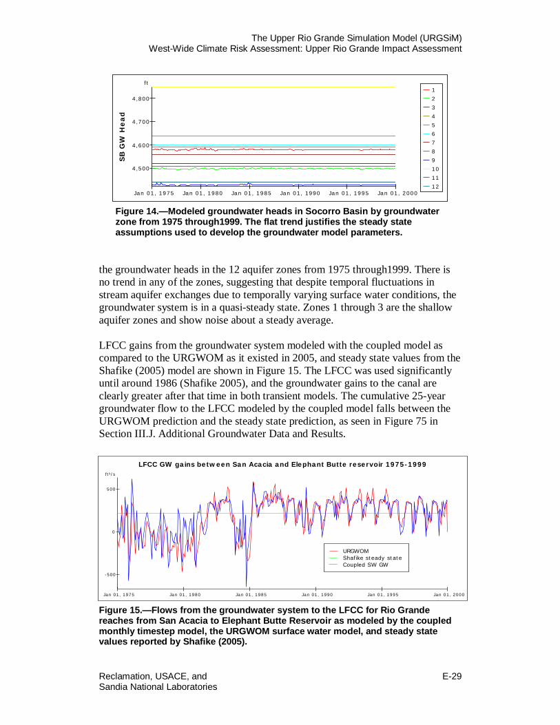
The Upper Rio Grande Simulation Model (URGSiM) West-Wide Climate Risk Assessment: Upper Rio Grande Impact Assessment
Reclamation, USACE, and E-29 Sandia National Laboratories
Figure 14.—Modeled groundwater heads in Socorro Basin by groundwater zone from 1975 through1999. The flat trend justifies the steady state assumptions used to develop the groundwater model parameters.
the groundwater heads in the 12 aquifer zones from 1975 through1999. There is no trend in any of the zones, suggesting that despite temporal fluctuations in stream aquifer exchanges due to temporally varying surface water conditions, the groundwater system is in a quasi-steady state. Zones 1 through 3 are the shallow aquifer zones and show noise about a steady average. LFCC gains from the groundwater system modeled with the coupled model as compared to the URGWOM as it existed in 2005, and steady state values from the Shafike (2005) model are shown in Figure 15. The LFCC was used significantly until around 1986 (Shafike 2005), and the groundwater gains to the canal are clearly greater after that time in both transient models. The cumulative 25-year groundwater flow to the LFCC modeled by the coupled model falls between the URGWOM prediction and the steady state prediction, as seen in Figure 75 in Section III.J. Additional Groundwater Data and Results.
Figure 15.—Flows from the groundwater system to the LFCC for Rio Grande reaches from San Acacia to Elephant Butte Reservoir as modeled by the coupled monthly timestep model, the URGWOM surface water model, and steady state values reported by Shafike (2005).
Jan 01, 1975 Jan 01, 1980 Jan 01, 1985 Jan 01, 1990 Jan 01, 1995 Jan 01, 2000
4,500
4,600
4,700
4,800
ft123456789101112
SB G
W H
ead
LFCC GW gains between San Acacia and Elephant Butte reservoir 1975-1999
Jan 01, 1975 Jan 01, 1980 Jan 01, 1985 Jan 01, 1990 Jan 01, 1995 Jan 01, 2000
-500
0
500
ft³/s
URGWOM Shafike steady state Coupled SW GW

The Upper Rio Grande Simulation Model (URGSiM) West-Wide Climate Risk Assessment: Upper Rio Grande Impact Assessment
E-30 Reclamation, USACE, and
Sandia National Laboratories
River leakage values from the different models are shown in Figure 16. The coupled values and URGWOM values agree well from 1985 on, but not before 1985. The URGWOM results shown here are from an obsolete model version developed around 2005 and are no longer relevant. From a cumulative river leakage perspective, the 25-year total river leakage predicted by the coupled model is similar to the steady state cumulative. The cumulative river leakage values are shown in Figure 76 in Section III.J. Additional Groundwater Data and Results.
Figure 16.—Rio Grande river leakage San Acacia to Elephant Butte Reservoir as modeled by the coupled monthly timestep model, the URGWOM surface water model, and steady state values reported by Shafike (2005). Riparian ET values predicted by the different models are shown in Figure 17, and cumulatively in Figure 77 in Section III.J. Additional Groundwater Data and Results. The large losses observed between San Acacia and San Marcial may be a result of gage errors, particularly between 1985 and 1988. However, analysis of systematic gage error is beyond the scope of URGSiM development, and so gage error is assumed to be normally distributed about zero and other methods are used to obtain mass balance at each gage from 1975 through 1999. In the case of the San Acacia to San Marcial reach, calibration of the coupled model was achieved by increasing riparian vegetation area in the reach by 33 percent. As a result of this calibration, the coupled values shown in Figure 17 are significantly higher than the URGWOM values. The surface water balance between San Acacia and San Marcial appears to be closed in URGWOM with large crop seepage rates as seen in Figure 18. In the coupled model, large seepage rates end up back in the drain system (i.e., the LFCC), and so cannot be used to close the surface mass balance. Since 2006 when these comparisons were made, URGWOM has changed significantly and been reworked to include a dynamic shallow groundwater component. As a result of this rework and several more years of observed behavior, the model dynamics and comparison of models between San Acacia and Elephant Butte Reservoir is due to be revisited.
River leakage between San Acacia and Elephant Butte reservoir 1975-1999
Jan 01, 1975 Jan 01, 1980 Jan 01, 1985 Jan 01, 1990 Jan 01, 1995 Jan 01, 2000
-500
0
500
ft³/s
URGWOM Shafike steady state Coupled SW GW

The Upper Rio Grande Simulation Model (URGSiM) West-Wide Climate Risk Assessment: Upper Rio Grande Impact Assessment
Reclamation, USACE, and E-31 Sandia National Laboratories
Figure 17.—Riparian ET between San Acacia and Elephant Butte Reservoir as modeled by the coupled monthly timestep model, the URGWOM surface water model, and steady state values reported by Shafike (2005).
Figure 18.—Crop seepage between San Acacia and Elephant Butte Reservoir as modeled by the coupled monthly timestep model and the URGWOM surface water model.
The last head-dependent flux of consideration for the historic period in the Socorro Basin groundwater system is canal leakage, which is modeled from San Acacia to San Marcial in the coupled model. It is not modeled explicitly in older versions of URGWOM and is not included in the steady state mass balance done by Shafike (2005). This is a relatively small flux in the coupled model, averaging a fairly steady 8 cfs.
Riparian ET between San Acacia and Elephant Butte reservoir 1975-1999
Jan 01, 1975 Jan 01, 1980 Jan 01, 1985 Jan 01, 1990 Jan 01, 1995 Jan 01, 20000
100
200
300
400
ft³/s URGWOM Shafike steady state Coupled SW GW
Crop seepage between San Acacia and San Marcial 1975-1999
Jan 01, 1975 Jan 01, 1980 Jan 01, 1985 Jan 01, 1990 Jan 01, 1995 Jan 01, 20000
50
100
150
200
ft³/s
URGWOM 12 Zone GW Model
The Upper Rio Grande Simulation Model (URGSiM) West-Wide Climate Risk Assessment: Upper Rio Grande Impact Assessment
E-32 Reclamation, USACE, and
Sandia National Laboratories
The spatially aggregated and coupled surface water/groundwater model of Socorro Basin is able to capture many of the temporal signals of the surface water system modeled by URGWOM as seen in Figure 15 and Figure 16, while maintaining a quasi-steady state groundwater mass balance as shown in Figure 14 and predicted by Shafike (2005). The combination of the surface and groundwater mass balance constraints suggest that either gage error led to significant overestimates of reach losses between 1985 and 1988 or the ET losses in that reach are larger than suggested by either URGWOM or Shafike’s (2005) steady state analysis. These conclusions support the value of basin scale multi-decadal analysis of coupled surface water groundwater systems as represented in URGSiM.
II.B. Surface Water Mass Balance
The Upper Rio Grande river system is fed primarily by snowmelt from the San Juan and Sangre de Cristo mountains, which define the northwestern and eastern boundaries of the basin respectively. Water moves into the river system via surface water inflows and return flows, groundwater seepage, and direct precipitation onto open water. Water is also diverted from the San Juan River system, through tunnels under the continental divide and into the Rio Chama system. This inter-basin water, moved from the Colorado Basin to the Rio Grande Basin, is known as San Juan Chama Project water. Water is lost from the river system by surface water diversions, leakage to the groundwater system, and open water evaporation to the atmosphere. Riparian evapotranspiration (ET) removes water from a shallow groundwater system, which is in relatively rapid exchange with the river. Water diverted for agricultural irrigation use can be lost to the groundwater system through conveyance system leakage (e.g., ditches and canals) and crop seepage, and to the atmosphere via crop ET and open water evaporation. In some reaches, groundwater discharges to the surface water system by seepage into agricultural drains. With respect to water balance, land use, and groundwater use, the river system within the model extent is significantly different above Cochiti Reservoir than it is below. In general, the reaches upstream of Cochiti Reservoir have less available bottom lands for irrigated agriculture and tend to gain surface water from groundwater and tributary inflows faster than surface water is lost to the atmosphere. Downstream of Cochiti Reservoir on the other hand, the river valley opens up—allowing more opportunity for irrigated agriculture and a net loss of surface water through the reaches. Figure 19 shows the observed accumulation of water upstream of Cochiti Reservoir and the net loss of water downstream from 1975 through 1999.

The Upper Rio Grande Simulation Model (URGSiM) West-Wide Climate Risk Assessment: Upper Rio Grande Impact Assessment
Reclamation, USACE, and E-33 Sandia National Laboratories
Figure 19.—Average river and agricultural conveyance flows through the Rio Grande system from 1975 through1999. In general, river gains above Cochiti and loses below. Otowi to below Cochiti reach appears to lose because of Cochiti Reservoir losses.
Most of the land that is practicably irrigable by surface water diversion and gravity application within the model extent lies below Cochiti Reservoir. As a result, significant amounts of water move through agricultural conveyance systems (i.e., canals, ditches, and drains) between Cochiti and Elephant Butte reservoirs, as shown in Table 11. Table 11.—Percent of Total Flow Past Points South of Cochiti Reservoir that is in Agricultural Conveyance System
Location Irrigation Season % Flows in Conveyance System 1975-99
August - October % Flows in Conveyance System 1975-99
Cochiti Pueblo 9% 19% San Felipe 3% 6% Albuquerque 12% 27% Bernardo 13% 32% San Acacia 22% 26% San Marcial 19% 34% Average 13% 23% Irrigation season is March through October. Flows in the conveyance system are a largest percent of total in the late summer and fall as river flows drop, but agricultural demand remains high. Data are from USGS gages listed in Table 2-2, as well as combined conveyance flow data from URGWOM model data (USACE et al. 2002).
Average Rio Grande river and agricultural conveyance flows 1975 -1999 as a function of distance downstream.
0
200000
400000
600000
800000
1000000
1200000
1400000
-50 0 50 100 150 200 250 300 350 400
Distance Downstream of Lobatos Gage [mile]
Ave
rage
Ann
ual F
low
in R
iver
and
C
onve
yanc
e St
ruct
ures
[af/y
r]
LobatosCerro
Taos Bridge
Embudo
Otowi
Costilla Creek Inflow s
Red River and Rio Pueblo de Taos Inflow s
Embudo Inflow s
Chama Inflow s
Cochiti Losses
Jemez Inflow s
Elephant Butte Losses
Albuquerque
Bernardo
Intensive ag use
Rio Puerco Inflow s

The Upper Rio Grande Simulation Model (URGSiM) West-Wide Climate Risk Assessment: Upper Rio Grande Impact Assessment
E-34 Reclamation, USACE, and
Sandia National Laboratories
II.B.1. River Reach Mass Balance
River Reach Inflows and Outflows Employing mass balance, the amount of water that flows out of a given river reach can be expressed mathematically as a function of inflows, outflows, and change in storage within the reach. At a monthly timestep, the change in storage in a river reach is assumed to be negligible with respect to the other flows through the reach, and precipitation gains to open water are also assumed to be negligible. The governing equation for a generic reach (j) is shown in Equation 3.
(3)
Where:
represents mainstem flow out of the bottom of reach j, which is the location of the gage representing the lower end of the reach.
represents mainstem flow into reach j, from the reach above or a gage on the model boundary. If reach i is immediately above reach j, the flow out of reach i is the same as the flow into reach j: .
represents the net sum of all interactions between the river and groundwater system in the reach, and is positive for a groundwater gaining reach, and negative for a groundwater losing reach.
represents open water evaporative losses.
represents the net sum of all surface water inflows into and diversions out of the reach, as shown in Equation 4 below.
(4)
The surface water inflows, diversions, and returns, may be gaged or ungaged. The terms represent gaged and ungaged surface water inflows (tributaries) and surface water diversions and returns respectively. The general strategy used to solve reach based mass balance (Equation 3) during the calibration period is to set the mainstem inflow term ( ) using historic gage data.
jevap
jgwsw
jsw
jm
jmsout QQQQQ −++= sin
jmsoutQ
jmQ sin
jm
imsout QQ sin=
jgwswQ
jevapQ
jswQ
jswreturn
jnswdiversio
jswungaged
jswgaged
jsw QQQQQ +−+=
jswreturn
jnswdiversio
jswungaged
jswgaged QQQQ ,,,
jmQ sin

The Upper Rio Grande Simulation Model (URGSiM) West-Wide Climate Risk Assessment: Upper Rio Grande Impact Assessment
Reclamation, USACE, and E-35 Sandia National Laboratories
Open water evaporation losses ( ) are estimated using reach area (section II.B.1.b. Reach Open Water Area). Reference ET calculated with the Hargreaves equation (Hargreaves and Samani, 1985) using historic temperature data and locally developed coefficients for relating reference ET to open water evaporation (see Section III: Evapotranspiration Calculations in URGSIM). The groundwater exchange ( ) is from a coupled, dynamic groundwater model, or a static exchange based on historic winter gage data, depending on data available for a given reach as described in section II.A. The surface water term ( ) is found using Equation 4, whose terms are set to historic gage values where available, and modeled otherwise. Crop ET losses for all reaches ( ) are modeled with the Hargreaves-based reference ET (see Section III: Evapotranspiration Calculations in URGSIM). In reaches where the river system and conveyance system are coupled to a groundwater model, calibration involves a combination of ungaged surface inflows and/or parameter adjustments associated with the surface water groundwater connection, to best match historic gage data. During validation and scenario evaluation:
• Main stem flows into the reach ( ) are set to gage data for reaches beginning on the model boundary, and to outflows from the reach above otherwise.
• Surface water diversions ( ) are modeled based on agricultural demand and historic diversion patterns.
All other terms in Equations 3 and 4 are calculated as in the calibration period. In most reaches, the ungaged surface water inflow term ( ) is used as a closure and calibration term. Table 12 summarizes important information associated with the modeled reaches, including degree of groundwater coupling. The carriage water factor is a calibration term for the agricultural conveyance system that limits how much of the water in the conveyance system is unavailable for depletion.
jevapQ
jgwswQ
jswQ
jcropETQ
jmQ sin
jnswdiversioQ
jswungagedQ

The Upper Rio Grande Simulation Model (URGSiM) West-Wide Climate Risk Assessment: Upper Rio Grande Impact Assessment
E-36 Reclamation, USACE, and
Sandia National Laboratories
Table 12.—Reach Summary Table
Reach Length (miles)
Gaged Tributaries
Irrigated Ag
Acreage Modeled (acres)
Carriage Water Factor
(%)
Riparian Acreage Modeled (acres)
Modeled Ag Conveyance
System
Coupled GW
Model
Chama: Willow Creek to Heron 12
Azotea Tunnel
(San Juan Chama)
0 0 None
Chama: Heron to El Vado 6 Rio Chama 0 1 None Chama: El Vado to Abiquiu 29 300 20 Static
Chama: Abiquiu to Chamita 29 Ojo
Caliente 4,540 80 Static
Lobatos to Cerro 26 Costilla Creek 0 300 Static
Cerro to Taos Junction Bridge 35
Red River Rio Pueblo
de Taos 0 0 Static
Taos Junction Bridge to Embudo 15 Rio
Embudo 190 100 Static
Embudo to Otowi 29 4,670 165 Dynamic Otowi to Cochiti 27 0 1 Dynamic
Cochiti to San Felipe 15 Galisteo Creek 4,520 0.85 4,055 X Dynamic
Jemez: Jemez Pueblo to Reservoir 30 5,370 0.2 3,985 X Dynamic
San Felipe to Albuquerque 33 North Flood
Channel 12,680 0.65 6,747 X Dynamic
Albuquerque to Bernardo 53 South Flood Channel 53,700 0.4 20,114 X Dynamic
Bernardo to San Acacia 14 Rio Puerco 680 0.2 6,639 X Dynamic San Acacia to San Marcial 48 10,490 0.2 21,591 X Dynamic
San Marcial to Elephant Butte 42 0 7,635 X Dynamic
Elephant Butte to Caballo 18 0 0 None Irrigated agricultural acreage is an average of 1975 through 1999 values reported in URGWOM physical model documentation (USACE et al. 2002) and information from Rio Chama watermaster report 2002 (Wells 2002). Riparian acreage is calculated from remotely sensed data for reaches above Cochiti Reservoir and URGWOM values below, with the exception of Jemez, which uses values from a regional groundwater model of the Albuquerque Basin by McAda and Barroll (2002).

The Upper Rio Grande Simulation Model (URGSiM) West-Wide Climate Risk Assessment: Upper Rio Grande Impact Assessment
Reclamation, USACE, and E-37 Sandia National Laboratories
Reach Open Water Area The open water area associated with each reach of the river channel is a function of flow rate and channel cross-section geometry. Above Cochiti Reservoir, the relationship between stream width and flow associated with each gage is used as a proxy for the relationship in associated reaches. Channel geometry at gage locations is not likely representative of the entire reach above or below the gage, but additional data are not readily available, and surface evaporation from the upper reaches is conceptually a relatively small term, so this assumption is considered acceptable. The cross-sectional area at each gage as a function of flow rate is reported in the URGWOM Physical Model Documentation (USACE et al. 2002). Stage as a function of flow rate is a key relationship associated with surface water gages, and is available indirectly from field measurement data published online for each gage operated by the United States Geological Survey (USGS).7 With stage and cross-sectional area available as a function of flow rate, a trapezoidal channel cross section was assumed, and a base width and bank slope selected to fit the relationships between flowrate, stage, and cross-sectional area observed at the gages. Table 13 summarizes cross-sectional relationships adopted for select gages above Cochiti Reservoir. Table 13.—Channel Geometry Relationships Adopted at Selected Gages, Used to Estimate Stage and Area as a Function of Flow Rate in Reaches above Cochiti Reservoir. Reaches between gages in this table used an average of both; other reaches used upper or lower gage data as available.
Gage Stage (ft))
from Q (cfs)
Cross Sectional Area
(ft2) Fitted Base Width
Parameter (ft))
Fitted Bank Slope
Parameter (run/rise)
(-) from Q (cfs) Rio Chama below El Vado 0.27*Q0.37 13*Q0.48 75 8 Rio Chama above Abiquiu Reservoir 0.35*Q0.36 11.5*Q0.47 50 5 Rio Chama below Abiquiu Dam 0.4*Q0.33 7*Q0.54 28 12
Rio Grande near Cerro 0.2145*Q0.4742 4.2943*Q0.6976 56 6.5 Rio Grande at Embudo 0.15*Q0.48 5.1771*Q0.593 61 3 Rio Grande at Otowi 0.2*Q0.41 3.2959*Q0.6628 40 16
7 This is online at < http://nwis.waterdata.usgs.gov > (e.g., the web site for Rio Grande near Cerro gage is: <http://nwis.waterdata.usgs.gov/nm/nwis/measurements/?site_no=08263500&agency_cd=USGS>.)

The Upper Rio Grande Simulation Model (URGSiM) West-Wide Climate Risk Assessment: Upper Rio Grande Impact Assessment
E-38 Reclamation, USACE, and
Sandia National Laboratories
A trapezoidal channel did not satisfactorily describe historic field measurements of stage and flow at either the Rio Grande gage below Taos Junction Bridge or the Chama gage near Chamita, and so these gages were not included. Chama reaches from below El Vado Reservoir and all Rio Grande reaches above Cochiti Reservoir were assumed to follow the cross-sectional relationships of the gages defining the beginning or end of the reach, or an average of both as available. For example, in the reach from Lobatos to Cerro, for an average monthly flow rate of 100 cubic feet per second (cfs), the calculated river stage using the Cerro gage relationship would be 0.2145*100 0.4742 = 1.9 feet. The calculated width of the river would be 56 feet (base width parameter) plus 6.5 (bank slope parameter)*1.9 feet, or 68.35 feet. This width is then multiplied by the length of the reach (26 miles, see Table 12) to get a total open water area of 0.34 square miles for Lobatos to Cerro at 100 cfs flowrate. A trapezoidal channel did not satisfactorily describe historic field measurements of stage and flow at either the Rio Grande gage below Taos Junction Bridge or the Chama gage near Chamita, and so these gages were not included. Rio Chama reaches from below El Vado Reservoir and all Rio Grande reaches above Cochiti Reservoir were assumed to follow the cross-sectional relationships of the gages defining the beginning or end of the reach, or an average of both as available. For example, in the reach from Lobatos to Cerro, for an average monthly flow rate of 100 cfs, the calculated river stage using the Cerro gage relationship would be 0.2145*100 0.4742 = 1.9 feet. The calculated width of the river would be 56 feet (base width parameter) plus 6.5 (bank slope parameter)*1.9 feet, or 68.35 feet. This width is then multiplied by the length of the reach (26 miles, see Table 12) to get a total open water area of 0.34 square miles for Lobatos to Cerro at 100 cfs flowrate. Below Cochiti Reservoir, the open water area associated with each reach of the river is calculated using flow based relationships developed by the URGWOM technical team (USACE et al. 2002), shown in Table 14. Table 14.—Open Water Area of Reaches below Cochiti Reservoir as a Function of River Flow. Relationships from URGWOM (USACE et al. 2002) physical model documentation page 39.
River Reach River Area (acres)as a Function
of Flowrate (Q) in cfs Bank Full Area
(acres) Cochiti to San Felipe 110.85Q0.1988 625 San Felipe to Albuquerque 84.281Q0.4099 2718 Albuquerque to Bernardo 123.87Q0.4375 5175 Bernardo to San Acacia 12.828Q0.5291 1054 San Acacia to San Marcial 158.29Q0.3197 2913 San Marcial to Elephant Butte 60.722Q0.5293 166

The Upper Rio Grande Simulation Model (URGSiM) West-Wide Climate Risk Assessment: Upper Rio Grande Impact Assessment
Reclamation, USACE, and E-39 Sandia National Laboratories
II.B.2. Agricultural Conveyance Mass Balance Below Cochiti Reservoir, the agricultural conveyance system is modeled as a parallel unit of mass balance to the river system. For these reaches, the diversion and return flow terms in Equation serve as inflows and outflows for the conveyance system. Assuming that direct evaporation losses from conveyance features is negligible, mass balance in the conveyance system south of Cochiti Reservoir is modeled using Equation 5.
(5)
Equation 5 states that surface water can enter the conveyance system by diversion from the associated reach ( ), or by through flow from the conveyance system immediately upstream ( ). Water is lost from the conveyance system
to the atmosphere by ET from crops ( ). Conveyance water moves to the groundwater system as seepage from crops and canals, or moves from the groundwater system back to the conveyance system as seepage into drains. The groundwater exchange terms are lumped into a single conveyance to groundwater term ( ) in Equation 5 that can be positive or negative, depending on the relative magnitude of the conveyance to groundwater system exchanges. Surface water flows out of the conveyance system to the river ( ) or to the downstream conveyance system ( ).
The conveyance system is modeled using historic diversion ( ) and
through flow ( , ) data, and solving for unknown return flows
( ) after evaporative losses and groundwater exchanges are accounted for. Groundwater to conveyance system flows ( ) are modeled with a coupled groundwater model (Section 3.A.i: Modified Penman ET0 Problems), leaving return flows ( ) as the only unknown to be solved for using Equation 5. Water available to return ( ) or to flow into the next conveyance reach
( , ) is partitioned based on reach-specific historic proportions developed for the calibration period and used for all other modeling periods.
II.B.3. Reservoir Mass Balance Seven reservoirs are included in the model. Table 15 summarizes basic information associated with the reservoirs. Reservoir mass balance is calculated according to Equation 6.
jconvtf
jswreturn
jconvgw
jcropET
iconvtf
jnswdiversio QQQQQQ +++=+
jnswdiversioQ
iconvtfQ
jcropETQ
jconvgwQ
jswreturnQ
jconvtfQ
jnswdiversioQ
iconvtfQ j
convtfQj
swreturnQj
convgwQ
jswreturnQ
jswreturnQ
iconvtfQ j
convtfQ
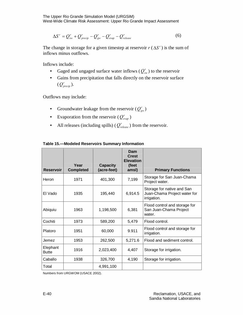
The Upper Rio Grande Simulation Model (URGSiM) West-Wide Climate Risk Assessment: Upper Rio Grande Impact Assessment
E-40 Reclamation, USACE, and
Sandia National Laboratories
(6)
The change in storage for a given timestep at reservoir r ( ) is the sum of inflows minus outflows. Inflows include:
• Gaged and ungaged surface water inflows ( ) to the reservoir • Gains from precipitation that falls directly on the reservoir surface
( ).
Outflows may include:
• Groundwater leakage from the reservoir ( )
• Evaporation from the reservoir ( )
• All releases (including spills) ( ) from the reservoir.
Table 15.—Modeled Reservoirs Summary Information
Reservoir Year
Completed Capacity
(acre-feet)
Dam Crest
Elevation (feet amsl) Primary Functions
Heron 1971 401,300 7,199 Storage for San Juan-Chama Project water.
El Vado 1935 195,440 6,914.5 Storage for native and San Juan-Chama Project water for irrigation.
Abiquiu 1963 1,198,500 6,381 Flood control and storage for San Juan-Chama Project water.
Cochiti 1973 589,200 5,479 Flood control.
Platoro 1951 60,000 9.911 Flood control and storage for irrigation.
Jemez 1953 262,500 5,271.6 Flood and sediment control.
Elephant Butte 1916 2,023,400 4,407 Storage for irrigation.
Caballo 1938 326,700 4,190 Storage for irrigation.
Total 4,991,100 Numbers from URGWOM (USACE 2002).
rrelease
revap
rgw
rprecip
rsw
r QQQQQS −−−+=∆
rS∆
rswQ
rprecipQ
rgwQ
revapQ
rreleaseQ
The Upper Rio Grande Simulation Model (URGSiM) West-Wide Climate Risk Assessment: Upper Rio Grande Impact Assessment
Reclamation, USACE, and E-41 Sandia National Laboratories
In general, as will be discussed in more detail in the following sections, reservoirs were calibrated with historic gaged surface water inflows and releases, as well as calculated precipitation, evaporation, and groundwater leakage. Reservoir releases were set to historic for the calibration period and modeled with operation rules for the validation and scenario evaluation periods. The following sections describe each of the terms in Equation 6 in more detail.
Reservoir Area URGSiM is a mass balance based model and thus tracks the volume of water in each reservoir to start each timestep. Reservoir areas are calculated based on storage volume in the reservoir using Elevation-Area-Capacity relationships specific to each reservoir. Ice cover on a given reservoir is a historically measured value, taken from the daily URGWOM data set and averaged to monthly. For scenario evaluation runs, the ice cover is calculated using a simple regression relationship to average air temperature during the previous month.
Reservoir Evaporation Reservoir precipitation gains for all reservoirs are calculated as the evaporation rate at a given reservoir in a given timestep multiplied by the reservoir area to start that timestep. For the 1975 through 1999 period, pan evaporation was measured for April through October for the five reservoirs north of Albuquerque where evaporation pans freeze, and during all months for Elephant Butte and Caballo reservoirs. For the five upper reservoirs, where pan evaporation cannot be consistently measured from November through March, winter evaporation rate is estimated by Equation 7.
(7)
Where:
= evaporation rate from reservoir r during month m [L/T] = average daily maximum temperature for r during m [degree]
= average daily minimum temperature for r during m [degree] = coefficient of proportionality for r during m [L/(degree*T)]
values are constant for a given reservoir in a given month, and are shown for
reservoirs above Elephant Butte Reservoir in Table 16.
mrmrmr
mr kTT
E ,,
min,
max, *2+
=
mrE ,
mrT ,max
mrT ,min
mrk ,
mrk ,

The Upper Rio Grande Simulation Model (URGSiM) West-Wide Climate Risk Assessment: Upper Rio Grande Impact Assessment
E-42 Reclamation, USACE, and
Sandia National Laboratories
Table 16.—Winter Reservoir Coefficient of Proportionality ( ) for the Five Upper Reservoirs
Reservoir
(ft/°F/month)
Month
Nov Dec Jan Feb Mar
Heron, El Vado, and Abiquiu 0.0035 0.0026 0.0031 0.0037 0.006
Cochiti and Jemez 0.0047 0.0032 0.0038 0.0046 0.0074
For the five upper reservoirs from April through October, and Elephant Butte and Caballo reservoirs during all months, evaporation rate is estimated with Equation 8 .
(8)
Where:
= evaporation rate from reservoir r during month m [L/T] = pan evaporation measured at reservoir r during m [L/T]
Temperature and edge effects result in pan evaporation rates that are typically greater than actual open water evaporation rates. To correct for this effect, actual open water evaporation rate is estimated by multiplying measured pan evaporation by a pan coefficient less than unity. URGWOM uses a pan coefficient of 0.7 for all reservoirs. The methodology represented by Equations 7 and 8 for a monthly timestep is the same as used by URGWOM at a daily timestep (USACE et al. 2002).
Reservoir Precipitation Reservoir precipitation gains for all reservoirs are calculated as the measured precipitation depth at a given reservoir in a given timestep multiplied by the reservoir area to start that timestep. The precipitation gains go directly into storage in the given reservoir as shown in Equation 9.
(9)
Where:
= precipitation gains to reservoir r as defined in equation 4 [L3/T] = precipitation rate measured at reservoir r during month m [L/T]
mrk ,
mrk ,
mrpan
mr EE ,, *7.0=
mrE ,
mrpanE ,
)cov1(** ,,, mrmrmrrprecip APQ −=
rprecipQ
mrP ,

The Upper Rio Grande Simulation Model (URGSiM) West-Wide Climate Risk Assessment: Upper Rio Grande Impact Assessment
Reclamation, USACE, and E-43 Sandia National Laboratories
= the area of reservoir r during month m [L2] = percent of reservoir r covered by ice during month m [%]
Reservoir Groundwater Leakage Groundwater flow into Elephant Butte Reservoir is modeled from the Socorro Basin groundwater system as described in Section II.A: URGSiM Groundwater Mass Balance. Reservoir leakage is modeled for Heron, Cochiti, and Jemez reservoirs. Leakage from Heron Reservoir is modeled according to URGWOM (USACE et al. 2002) methodology (Equation 10).
(10)
Where:
= groundwater leakage out of Heron Reservoir [L3/T]. = the greater of 7,100 feet or the stage of Heron Reservoir in feet for
month m [L]. Reservoir leakage from Cochiti and Jemez reservoirs are calculated as a function of reservoir stage and underlying aquifer head as described in Roach and Tidwell (2009).
Reservoir Inflows Inflows to Heron Reservoir from the San Juan-Chama Diversion Tunnel are modeled for all time periods (see Section III.H.1. San Juan-Chama Diversions to Azotea Tunnel Outlet). Inflows to El Vado from Heron and Abiquiu reservoirs from the Rio Chama are set to appropriate gage data for the calibration period and modeled for validation and scenario runs. Inflows to reservoirs are modeled:
• El Vado Reservoir from the Rio Chama
• Cochiti Reservoir from the Rio Grande
• Jemez Reservoir from the Jemez River
Inflows to Elephant Butte and Caballo reservoirs from the Rio Grande are modeled based on reach behavior between the nearest upstream gage and the reservoir. If the nearest upstream gage is a calibration gage (Table 3), it is set to observed values for the historic calibration period, and modeled values for validation and scenario evaluation. Input gages (Table 2) are set to observed values for all periods, and specified for scenarios as a reshuffle of historic data or
mrA ,
mr ,cov
sft
sftftzQ mHeronHeron
gw
32, 76.02134.0*)7100( +−=
HerongwQ
mHeronz ,

The Upper Rio Grande Simulation Model (URGSiM) West-Wide Climate Risk Assessment: Upper Rio Grande Impact Assessment
E-44 Reclamation, USACE, and
Sandia National Laboratories
in some other manner. Reservoir inflows from modeled but ungaged reaches are calculated within the model for all periods. Ungaged inflows were added to Heron and Abiquiu reservoirs for calibration purposes.
In addition to modeled or gaged reservoir inflows, an error inflow (positive or negative at each timestep but net zero over time after calibration) is added to the reservoirs at each calibration timestep to force the modeled storage to observed storage. This error term is added to the reservoir to avoid compounding errors and maintain reservoir storage at historic observed levels during the calibration period.
Reservoir Releases Reservoir releases for the 1975 through 999 calibration period are set to observed historic releases. Reservoir releases for the validation and scenario evaluation periods are modeled using reservoir operation rules. The seven major reservoirs within the model extent are operated according to a complex set of legal and physical constraints with a broad range of objectives, including:
• Interstate compact delivery requirements • Downstream flood control • Storage for agricultural and municipal demand • Electric generation • Minimum stream flow
The full extent of operational requirements is represented in URGWOM. Predicted behavior of reservoirs under specific hydrologic scenarios by URGWOM was used to develop a simplified set of rules for operations. The reservoir operations rules that determine releases in the validation and scenario evaluation periods are described in Section III.F. Reservoir Operations in URGSiM.
III. Evapotranspiration Calculations in URGSiM
In 2011, URGSiM switched from a modified Penman based Reference Evapotranspiration (ETo) equation with an associated growing degree day based crop coefficient method and 20 vegetation types, to a Hargreaves-based ETo equation, Food and Agriculture Organization of the United Nations Irrigation and Drainage Paper 56 ( FAO-56) based crop coefficients (Allen et al. 1998), and 5 vegetation types. These changes were made for a variety of reasons including: unreliable results from the previous methods, sparse and unreliable historic

The Upper Rio Grande Simulation Model (URGSiM) West-Wide Climate Risk Assessment: Upper Rio Grande Impact Assessment
Reclamation, USACE, and E-45 Sandia National Laboratories
weather data, and unnecessary complexity in previous vegetation classifications. This section summarizes the rationale for these changes and the implications in terms of simulated ET in the Upper Rio Grande between 1975 and 1999.
III.A. Reference Evapotranspiration (ET) Equations
URGSiM (Roach 2007 and Roach and Tidwell 2009) calculates a monthly mass balance in reaches of the Upper Rio Grande in New Mexico from 1975 through 1999 in calibration mode, 2000 through 2009 in validation mode, and 2010 forward in scenario analysis mode. ET is one of the major terms in this mass balance and is calculated as the smaller of potential ET and available water. For a given month, reach, and vegetation type, this can be expressed mathematically as shown in Equation 11 below.
𝐸𝑇𝑎𝑟,𝑚,𝑣 = min (𝐸𝑇𝑝
𝑟,𝑚,𝑣 ,𝐻2𝑂𝑎𝑣𝑎𝑖𝑙𝑎𝑏𝑙𝑒𝑟,𝑚,𝑣 ) (11)
Where: 𝐸𝑇𝑎
𝑟,𝑚,𝑣 [L3/T] = actual ET 𝐸𝑇𝑝
𝑟,𝑚,𝑣 [L3/T] = potential ET 𝐻2𝑂𝑎𝑣𝑎𝑖𝑙𝑎𝑏𝑙𝑒
𝑟,𝑚,𝑣 [L3/T] = water available for ET in reach r during month m for vegetation type v. Vegetation types include irrigated crops, riparian vegetation, or open water as discussed further in Section III.B. Crop Coefficients. In URGSiM, water availability is determined for:
• Irrigated crops as a fraction of monthly rainfall (effective precipitation) plus irrigation deliveries to the field
• Riparian vegetation by the depth to groundwater
• Open water by river flow or reservoir volume
Potential ET is calculated as Reference ET (ETo) multiplied by a crop coefficient and an area expressed mathematically in Equation 12 below.
𝐸𝑇𝑝
𝑟,𝑚,𝑣 = 𝐸𝑇𝑜𝑟,𝑚 ∗ 𝐾𝑐
𝑟,𝑚,𝑣 ∗ 𝐴𝑟,𝑚,𝑣 (12)
Where: 𝐸𝑇𝑜
𝑟,𝑚 [L/T], the reference ET, is the potential ET of a reference crop, either grass or Alfalfa in reach r during month m

The Upper Rio Grande Simulation Model (URGSiM) West-Wide Climate Risk Assessment: Upper Rio Grande Impact Assessment
E-46 Reclamation, USACE, and
Sandia National Laboratories
𝐾𝑐𝑟,𝑚,𝑣 [-] is a crop coefficient that relates the potential ET of crop v to the
reference crop 𝐴𝑟,𝑚,𝑣 [L2] is the area of vegetation v in reach r during month m. Estimation of vegetative area (𝐴𝑟,𝑚,𝑣), although potentially uncertain, is straightforward. Estimation of 𝐸𝑇𝑜
𝑟,𝑚 and 𝐾𝑐𝑟,𝑚,𝑣 ,on the other hand, are uncertain
and also ambiguous. There are a variety of equations and methods available in the literature for calculating ETo, crop coefficients, or the product of the two. These range from highly localized pan evaporation observations to temperature and radiation based equations (e.g., Hargreaves 1985) to more general data intensive semi-empirical equations (e.g. Penman-Monteith as described in Allen et al. (1998).
III.A.1. Modified Penman ETo Problems Prior to 2011, following Reclamation’s ET Toolbox (Brower 2008), URGSiM used a version of the Penman equation modified by Dr. Ted Sammis (Sammis et al. 1985) to estimate ETo and an associated growing degree day based crop coefficient estimation (Sammis et al. 1985). In 2011, the ET Toolbox abandoned the Sammis-modified Penman method for calculating ETo because of erroneously high results. ETo for year 2007 Angostura weather station data (Reclamation 2012) was calculated with a variety of equations by Keller-Bliesner Engineering using software developed by Dr. Rick Allen called Ref-ET. According to this analysis, the annual cumulative ETo calculated by the modified Penman equation was approximately 80 inches, some 20 inches or 33 percent greater than the approximately 60 inches calculated by the widely accepted FAO-56 (Allen et al. 1998) or American Society of Civil Engineers (ASCE) Standard (Task Committee on Standardization of Reference Evapotranspiration 2005) methods. Angostura in 2007 was the gage and period of time singled out for intensive comparison of various equations for calculating ETo. Though the Angostura results are not applicable quantitatively to all weather stations and all years they follow a qualitative pattern of significant overestimate of ETo by the modified Penman equation.
III.A.2. Choosing a New ETo Calculation The results described above led to the abandonment of the legacy modified Penman equation as the default method of ETo calculation by URGSiM, URGWOM, and the ET Toolbox. In choosing a new method for URGSiM, the availability and quality of historic data became of concern. Generally, two forms of the Penman-Monteith equation (FAO-56 [Allen, et al. 1998], and the ASC Standard method [Task Committee on Standardization of Reference Evapotranspiration 2005]) are the current state of the art for calculating ETo where sufficient high quality data exists.

The Upper Rio Grande Simulation Model (URGSiM) West-Wide Climate Risk Assessment: Upper Rio Grande Impact Assessment
Reclamation, USACE, and E-47 Sandia National Laboratories
Figure 20.—Cumulative Reference ET (ETo) calculated at Angostura weather station during the year 2007 by a variety of ETo equations. The modified Penman used previously by the ET Toolbox is erroneously high compared to all other methods. The other high outlier, the FAO-24 Penman has been superseded by the FAO-56 Penman-Monteith method. The FAO-56 and ASCE Standard methods are coincident for this data. The Hargreaves 1985 method requires temperature data only. Penman-Monteith based equations such as these are weather data intensive; however, requiring solar radiation, wind speed, temperature, and relative humidity data. If these data are not available, or of questionable quality, then less data intensive temperature based methods such as the Hargreaves 1985 (Hargreaves and Samani 1985) may be more appropriate. In the Rio Grande Valley in New Mexico upstream of Caballo Reservoir (the area in which URGSiM requires ETo), from 1975 through 1999 (the calibration period for URGSiM), full weather data including solar radiation, wind speed, and relative humidity measurements are spatially limited and of suspect quality. Temperature measurements, on the other hand, are more widely available and reliable. In addition, the monthly timestep of URGSiM reduces temporal variability that would be captured by a more complex and data intensive method, which reduces the advantage of the more complex method. Indeed, for timesteps longer than 5 days, the Hargreaves 1985 equation often compares very favorably to more complex methods (Hargreaves and Allen 2003). For all of these reasons, the relatively simple Hargreaves 1985 equation (Equation 13) was adopted for use by URGSiM:

The Upper Rio Grande Simulation Model (URGSiM) West-Wide Climate Risk Assessment: Upper Rio Grande Impact Assessment
E-48 Reclamation, USACE, and
Sandia National Laboratories
𝐸𝑇𝑜 = 0.0023 𝑅𝑎 (𝑇𝑚𝑒𝑎𝑛+ 17.8) (𝑇𝑚𝑎𝑥− 𝑇𝑚𝑖𝑛)0.5
(13)
Where: Ra is extraterrestrial radiation expressed as a depth of evaporated water per time [L/T] Tmean, Tmin, and Tmax are the mean, minimum, and maximum temperatures in Celsius. For URGSiM, at a monthly timestep, Tmean is the average mean daily temperature for the month, and Tmin, and Tmax are the mean daily minimum and mean daily maximum temperatures for the month, respectively. Although the (𝑇𝑚𝑎𝑥 − 𝑇𝑚𝑖𝑛)0.5 term in Equation 13 is not linear, monthly ETo values calculated from monthly average inputs are almost identical to monthly averages of ETo values calculated from daily inputs (Figure 21) for daily Angostura weather station data from 2000 through 2011 (Reclamation 2012). The choice to use Hargreaves 1985 is further supported by data availability and quality issues in the region explained in more detail in the next two subsections.
Figure 21.—Comparison of monthly calculations of ETo in centimeters per day (cm/da) using the Hargreaves equation (x-axis) to monthly averages of daily calculations of ETo using the same (y-axis) shows an almost imperceptible difference between the two methods for 12 years of Angostura weather station data. This stability of the non-linear (𝑻𝒎𝒂𝒙 − 𝑻𝒎𝒊𝒏)𝟎.𝟓 term in the Hargreaves equation for daily versus monthly calculations suggests that daily (Tmax – Tmin) in °C is relatively constant in any given month.
The Upper Rio Grande Simulation Model (URGSiM) West-Wide Climate Risk Assessment: Upper Rio Grande Impact Assessment
Reclamation, USACE, and E-49 Sandia National Laboratories
Data Availability Issues Within the spatial extent of URGSiM, full weather data (i.e., temperature, wind speed, relative humidity, and solar radiation) are available from 1985 through 1992 and 1993 to present at the Los Lunas and Alcalde data stations (New Mexico State University nd). Weather data from additional locations became available starting in 2001; however, the 1975 through 1999 calibration period is the period of focus for this analysis. Thus for the period of interest, full weather data are not available at all for 11 of 25 years and are only available in two useful locations for the remaining 14 years. Temperature data, however, are more widely available. There are numerous temperature stations along the Upper Rio Grande or Rio Chama within the URGSiM model extent with data available beginning in 1975 or earlier. The locations of some of these are shown in Figure 22 along with the two full weather data sites. It is clear from this figure that without better spatial and temporal data availability, the potential benefit of a data-intensive, Penman-Monteith-based Reference ET method is questionable, and a temperature based method makes the most sense for historic calculations.
Data Quality Issues In addition to the spatial and temporal sparseness of the historic record for full weather data, preliminary analysis also suggests that the available historic data have not been carefully checked and may not be reliable. Keller-Bliesner performed a high level analysis of weather data for the Alcalde Station from 1985 through 2010, and found obvious issues with the solar radiation, relative humidity, and wind speed data. As seen in Figure 23, daily solar radiation values higher than theoretical maxima, relative humidity values greater than 100 percent or equal to 0 percent, and dramatic changes in wind sensor behavior in short periods of time were all noted in the data. In general, a model is only as good as the data driving it, and this applies to Reference ET equations. As stated in Appendix D of the ASCE Standardized Reference Evapotranspiration Equation documentation (Task Committee on Standardization of Reference Evapotranspiration 2005):
“Weather data must be screened before use in any ET equation, including the standardized equation, to ensure that data are of good quality and are representative of well-watered conditions. This is especially important with electronically collected data, since human oversight and maintenance may be limited. When weather measurements are determined to be faulty, they can be adjusted or corrected using a justifiable and defensible procedure.”

The Upper Rio Grande Simulation Model (URGSiM) West-Wide Climate Risk Assessment: Upper Rio Grande Impact Assessment
E-50 Reclamation, USACE, and
Sandia National Laboratories
Figure 22.—Weather station data available along river reaches within the URGSiM model extent with periods of record starting before the year 2000. Stations are labeled by period of record start year. Only two stations are available with long-term full weather data (Alcalde and Los Lunas), while numerous stations are available with long-term temperature data.

The Upper Rio Grande Simulation Model (URGSiM) West-Wide Climate Risk Assessment: Upper Rio Grande Impact Assessment
Reclamation, USACE, and E-51 Sandia National Laboratories
Figure 23.—Weather station diagnostics for Alcalde weather station daily data between 1985 and 2010. Daily solar radiation values greater than theoretic maximum (upper left), maximum relative humidity values greater than 100 percent and minimum relative humidity values equal to 0 percent for years at a time (upper right), and dramatic shifts to the slope of cumulative wind plots in different years (lower left) are indicative of sensor problems. The daily temperature range (lower right) seems fine. The limited availability of full weather data sets for the spatial and temporal extents of interest to URGSiM coupled with the monthly timestep of the model are sufficient to preclude use of a Penman-Monteith ETo equation in the monthly timestep for URGSiM. The apparent unreliability of the full weather data adds even more credence to the decision to use a temperature-based method. Of the temperature-based methods, the Hargreaves 1985 equation (Equation 13 above) is perhaps the most widely accepted and is now used in URGSiM for ETo calculations.
III.B. Crop Coefficients
Reference ET (ETo) is by definition the potential ET rate of a well-watered reference crop. Hargreaves 1985 and most other ETo methods use a grass of

The Upper Rio Grande Simulation Model (URGSiM) West-Wide Climate Risk Assessment: Upper Rio Grande Impact Assessment
E-52 Reclamation, USACE, and
Sandia National Laboratories
specific properties as the reference crop. From this ETo, which is a function of atmospheric conditions and reference crop physiology, the potential ET rates of other vegetation types can be inferred based on vegetation-specific factors called crop coefficients as introduced in Equation 12 above. A crop coefficient of 0.9 for a given crop in a given time period means that the ET from that crop will be 90 percent of reference crop ET. Crop coefficients typically vary with time because of changes in the crop phenology.8 Crop coefficients can be defined as a function of month, position in growing season, or climatic factors depending on the level of detail desired.
III.B.1. Issues with the Sammis et al. (1985) Crop Coefficients A significant factor in the ET Toolbox’s use of the modified Penman method as the default for estimation of ETo was the existence of locally developed crop coefficients based on this specific ETo formulation. Sammis et al. (1985) developed crop coefficients for alfalfa, cotton, corn, and sorghum at locations throughout New Mexico. The crop coefficients were calculated by comparing ET estimates for the crop using a mass balance method (non-weighing lysimeter) to the Reference ET calculated from weather data using the modified Penman equation discussed in Section III.A.1. Reference Evapotranspiration (ET) Equations. Rather than correlating the resulting crop coefficients to the day of year, however, the crop coefficient was correlated to the cumulative growing degree days. Growing degree days are a proxy of expected cumulative plant growth, calculated with daily temperature data and plant properties. In this way, crop coefficients were calculated as a function of crop stage rather than date. Using this method, the crop coefficient for a given crop may vary on a given day from year to year based on antecedent temperature conditions to that point in the year. For example, in a cold year, alfalfa in June may be smaller and use less water than the same field of alfalfa in June of a warmer year.
Magnitude It would be expected that an erroneously high ETo from the modified Penman equation (as shown in Section III.A.1. Reference Evapotranspiration (ET) Equations) would lead to erroneously low crop coefficients, and that in combination the errors would cancel and potential ET estimates would be useful. However, as shown in Figure 24 and Figure 25, the opposite is true, at least for Angostura 2007 data. Figure 24 shows that Sammis et al. crop coefficients for alfalfa at Angostura in 2007 are higher than alfalfa crop coefficients of the magnitude of FAO-56 recommendations, particularly during the peak of the summer when ETo values are highest. When the effect of the growing degree day based crop coefficients are combined with the effect of the high ETo, the result, for the Angostura 2007 case, is potential ET estimates of 64 inches per year, which is
8 Crop phenology is the study of periodic plant and animal life cycle events.

The Upper Rio Grande Simulation Model (URGSiM) West-Wide Climate Risk Assessment: Upper Rio Grande Impact Assessment
Reclamation, USACE, and E-53 Sandia National Laboratories
Figure 24.—Crop coefficients calculated for alfalfa at Alcalde weather station using the Sammis et al. (1985) growing degree day (GDD) method compared to simple FAO-56 based estimates of 0.4 for the first month of the growing season and 0.95 thereafter. The growing degree day method values are higher than the FAO-56 based values from May 21st through September 19th, a nearly 4 month period during which Reference ET will be at its greatest. almost 50 percent higher than the 43 inches per year estimated for the FAO-56 ETo and crop coefficients case. Of this 21-inch-per-year difference, 15 inches (over 70 percent) is due to the ETo difference, and the remaining 6 inches is due to the crop coefficient difference. These results are shown graphically in Figure 25.
Also shown in Figure 25 is cumulative actual ET estimated by eddy covariance tower9 for an alfalfa field in San Acacia, which is further south and at a lower elevation than Angostura. Potential ET assumes “standard” growing conditions, meaning a disease free, well-fertilized crop, grown in large fields under optimum soil water conditions (Allen et al. 1998). This situation typically represents an upper limit to ET, and thus actual ET is often less than potential ET. Thus, a
9 Data downloaded 6/24/2010 from <http://bosque.unm.edu/~cleverly/ALF/ALF.html>. Website is no longer available as of 1/10/2012.
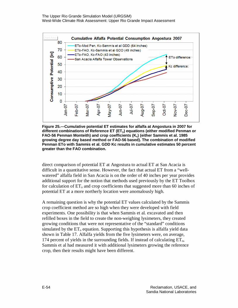
The Upper Rio Grande Simulation Model (URGSiM) West-Wide Climate Risk Assessment: Upper Rio Grande Impact Assessment
E-54 Reclamation, USACE, and
Sandia National Laboratories
Figure 25.—Cumulative potential ET estimates for alfalfa at Angostura in 2007 for different combinations of Reference ET (ETo) equations (either modified Penman or FAO-56 Penman Monteith) and crop coefficients (Kc) (either Sammis et al. 1985 growing degree day based method or FAO-56 based). The combination of modified Penman ETo with Sammis et al. GDD Kc results in cumulative estimates 50 percent greater than the FAO combination. direct comparison of potential ET at Angostura to actual ET at San Acacia is difficult in a quantitative sense. However, the fact that actual ET from a “well-watered” alfalfa field in San Acacia is on the order of 40 inches per year provides additional support for the notion that methods used previously by the ET Toolbox for calculation of ETo and crop coefficients that suggested more than 60 inches of potential ET at a more northerly location were anomalously high. A remaining question is why the potential ET values calculated by the Sammis crop coefficient method are so high when they were developed with field experiments. One possibility is that when Sammis et al. excavated and then refilled boxes in the field to create the non-weighing lysimeters, they created growing conditions that were not representative of the “standard” conditions simulated by the ETo equation. Supporting this hypothesis is alfalfa yield data shown in Table 17. Alfalfa yields from the five lysimeters were, on average, 174 percent of yields in the surrounding fields. If instead of calculating ETo, Sammis et al had measured it with additional lysimeters growing the reference crop, then their results might have been different.

The Upper Rio Grande Simulation Model (URGSiM) West-Wide Climate Risk Assessment: Upper Rio Grande Impact Assessment
Reclamation, USACE, and E-55 Sandia National Laboratories
Table 17.—Reference ET (ETo), Actual ET (Eta) in Non-Weighing Lysimeters, and Yields in the Lysimeters and Surrounding Field Crop Yields Reported by Sammis et al (1985) for Alfalfa
Location ETo
(mm) ETa
(mm) Alfalfa Yield (kg/ha)
Lysimeter Field Artesia 2,140 1,873 23,400 13,450 Clovis 2,142 1,786 15,800 12,780 Farmington 1,582 1,581 14,700 6,720 Las Cruces 1 1,710 1,715 21,900 11,430 Las Cruces 2 1,893 1,687 2,2600 12,100
Average 1,893 1,728 19,680 11,296 Note that lysimeter yields are significantly larger than field yields for all locations, with lysimeter yields averaging 174 percent of field yields. The non-weighing lysimeters were not representative of field conditions, and may not have been representative of “standard” conditions. kg/ha = kilogram per hectare mm = millimeter
Growing Degree Day Issues A final issue that has been noted with the use of growing degree day to estimate riparian crop coefficients is situations in which the growing degree day method begins to shut the plant down before the end of the growing season. This is illustrated when growing degree days are calculated using temperature data from the Bosque del Apache temperature station (Western Regional Climate Center 2013) and then translated to salt cedar crop coefficients using the growing degree day method in ET Toolbox (Brower 2008). The result, shown in Figure 26 is a crop coefficient that is zero before October 10 in every year between 2000 and 2008, before salt cedar is done transpiring (the ET Toolbox suggests a transpiration end date of November 15th for Salt Cedar). The ET Toolbox growing degree day versus crop coefficients curves shut down salt cedar and cottonwood ET by the time they reach 1,600 growing degree days, which is less than any other crop in the ET Toolbox for which crop coefficients is used except spring barley. Alfalfa is still transpiring at 4,000 growing degree days, and wheat at 3,000 to give some comparison. (The base temperature is higher for the riparian species than the other crops, meaning that the riparian species’ growing degree days will not accumulate as fast, so the comparison is not quite direct, but illustrative nonetheless).
10 These results are calculated at a monthly timestep using URGSiM, however because GDD days are calculated as the midpoint between daily max and daily min temperatures less a base temperature, the sum of daily calculated GDD will be the same as a single calculation with monthly average min and monthly average max temperatures.

The Upper Rio Grande Simulation Model (URGSiM) West-Wide Climate Risk Assessment: Upper Rio Grande Impact Assessment
E-56 Reclamation, USACE, and
Sandia National Laboratories
Figure 26.—Crop coefficient (Kc) estimated for Salt Cedar at the Bosque del Apache temperature station4 using a Growing Degree Method. Note that Kc comes down too quickly at the end of the summer mathematically shutting off ET prematurely before October of almost every year between 2000 and 2009. According to the ET Toolbox documentation (Brower 2008) page 34, the salt cedar and cottonwood growing degree day-to-crop-coefficient relationships are a result of “extensive field studies in 1999 at the Bosque Del Apache National Wildlife Refuge” by Dr. Salim Bawazir of NMSU. Interestingly, as can be seen in Figure 27, 1999 had low average temperatures at Bosque del Apache especially in April, June, and July compared to 2000 through 2011. Thus defining growing degree days- to-crop-coefficient relationships based on a single (relatively cool) year of data may explain why those curves end at 1,600 growing degree days but growing degree day values exceeding this are reached at Bosque del Apache by October of all but one year between 2000 and 2009. Regardless of the reason, the GDD based crop coefficients used previously by URGWOM and URGSiM can lead to obviously erroneous results for riparian vegetation in the (warmer) southern reaches of the Middle Rio Grande.
III.B.2. Current Crop Coefficient Methods
Irrigated Agriculture Irrigated agriculture in the URGSiM model extent has been dominated during recent history by alfalfa and pasture grass (see Section.III.C. Vegetation Classifications). To choose a new crop coefficient methodology for use in

The Upper Rio Grande Simulation Model (URGSiM) West-Wide Climate Risk Assessment: Upper Rio Grande Impact Assessment
Reclamation, USACE, and E-57 Sandia National Laboratories
Figure 27.—Monthly average temperature at the Bosque del Apache temperature station in 2000-2011 compared to the year 1999. Growing Degree Day based estimates of riparian crop coefficients in the ET Toolbox are based on 1999 field data from Bosque del Apache. 1999 was a cool summer in this location, especially in April, June, and July compared to 2000-2011. The “warmer” percentages mean that, for example, 100 percent of Aprils between 2000 and 2011 had higher average temperatures than April of 1999. URGSiM, observed ET data from the eddy covariance tower over an alfalfa field near San Acacia (data seen previously in Figure 25) was compared to potential ET calculated with a Hargreaves ETo method and alfalfa crop coefficients from three different sources, the Sammis et al. (1985) growing degree day method, the Middle Rio Grande Water Assessment (Reclamation 1997) values, and FAO-56 (Allen et al. 1998) based values. Results are seen in Figure 28 below. The actual ET is less than any of the potential ET values during the main growing season, but more than any method in October through December. The Sammis et al. (1985) growing degree day method results in the highest estimated potential ET while results from the MRGWA (reference) and FAO-56 (reference) crop coefficients are comparable. Based on this result, crop coefficient values based on FAO-56 were adopted for use in URGSiM for alfalfa, pasture grass, grains, and fruits and vegetables crop types. (The use of these four irrigated crop classifications is explained in Section III.C. Vegetation Classifications below.) The crop coefficients used are shown in Figure 29.

The Upper Rio Grande Simulation Model (URGSiM) West-Wide Climate Risk Assessment: Upper Rio Grande Impact Assessment
E-58 Reclamation, USACE, and
Sandia National Laboratories
Figure 28.—Estimates of potential ET for an alfalfa field near San Acacia during 2007. Blue line are estimates of actual ET from an eddy-covariance tower (see footnote #3). The red line is calculated ETo using the Hargreaves 1985 equation with observed temperature data from a temperature station next to the field. The remaining three lines are potential ET estimates resulting from multiplication of the ETo value by a crop coefficient for alfalfa for the given month from either the Sammis et al. (1985) GDD method, the Middle Rio Grande Water Assessment (MRGWA), or FAO-56 (Allen et al. 1998) based values.
Figure 29.—Tabular and visual representation of crop coefficients used by URGSiM.

The Upper Rio Grande Simulation Model (URGSiM) West-Wide Climate Risk Assessment: Upper Rio Grande Impact Assessment
Reclamation, USACE, and E-59 Sandia National Laboratories
Riparian Vegetation Figure 29 above also show values used for riparian vegetation, which are explained here. Riparian vegetation is vegetation growing along the river corridor which for the purposes of URGSiM is deep-rooted vegetation that can obtain water from the shallow ground water system (i.e., trees but not grasses), and is not irrigated. Eddy covariance tower measurements of actual ET from riparian vegetation are available in the Middle Rio Grande valley from 2000 through 2004 (Cleverly et al. 2006). Eddy covariance derived ET data from three locations representing sparse cottonwood, dense cottonwood, and salt cedar vegetation types is shown in Figure 30.
Figure 30.—Eddy covariance tower based monthly ET estimates for sparse cottonwood (blue), dense cottonwood (green), and salt cedar (red) vegetation types from 2000 through 2004. Shapes indicate the year of measurement, colors indicate vegetation type, and the solid lines represent vegetation specific average values. Average cumulative annual values (shown in inset) are approximately 41 inches for salt cedar, 42 inches for dense cottonwood, and 48 inches for sparse cottonwood.

The Upper Rio Grande Simulation Model (URGSiM) West-Wide Climate Risk Assessment: Upper Rio Grande Impact Assessment
E-60 Reclamation, USACE, and
Sandia National Laboratories
Modeling ET from riparian vegetation is complicated by reductions in potential ET as groundwater levels drop. Groundwater models typically specify some relationship between depth to groundwater and potential ET. In their Albuquerque Basin MODFLOW groundwater model, McAda and Barroll (2002) specify groundwater deeper than 30 feet (extinction depth) as inaccessible to riparian vegetation, and a maximum riparian ET of 5 feet per year when groundwater levels reach the ground surface. Baird and Maddock (2005) use a relationship between transpiration and groundwater depth that reflects decreases in plant activity for very shallow groundwater situations due to root inundation. As water levels approach the surface and transpiration shuts down (as shown by the Baird and Maddock [2005] line in Figure 31), direct evaporation from the ground surface should increase. For a spatially distributed model, it might be possible to separate transpiration and ground surface evaporation components, but for the spatially lumped URGSiM model, it would be difficult. To capture the transpiration peak in the Baird and Maddock (2005) line while including the deep extinction depth and direct evaporation for very shallow groundwater from McAda and Barroll (2002), URGSiM uses a combination of the two. The URGSiM relationship is shown along with those from McAda and Barroll (2002) and Baird and Maddock (2005) in Figure 31. Finally, to use reference ET information, URGSiM substitutes atmospheric potential ET for the absolute rates used by McAda and Barroll (2002) and Baird and Maddock (2005) (5 feet per year and 0.3 centimeters per day respectively). In this way, URGSiM combines both groundwater level and atmospheric condition information in the calculation of riparian ET. Adding the groundwater dependence to Equation 12, we get Equation 14:
𝐸𝑇𝑝𝑔𝑤𝑧,𝑚,𝑣 = 𝐸𝑇𝑜
𝑟,𝑚 ∗ 𝐾𝑐𝑚,𝑣 ∗ 𝐺𝑊𝑐
𝑔𝑤𝑧,𝑚,𝑣
∗ 𝐴𝑔𝑤𝑧,𝑚,𝑣 (14)
Where: 𝐸𝑇𝑝
𝑔𝑤𝑧,𝑚,𝑣 [L3/T] is evapotranspiration from riparian crop v in groundwater zone gwz during month m 𝐸𝑇𝑜
𝑟,𝑚 [L/T] is reference ET in reach r during month m 𝐾𝑐𝑚,𝑣 [-] is the riparian crop coefficient
𝐺𝑊𝑐
𝑔𝑤𝑧,𝑚,𝑣 [-] is the groundwater coefficient (percent of maximum ET due to groundwater depth) which is calculated with the depth to groundwater in groundwater zone gwz during month m, and the URGSiM relationship shown in Figure 31 𝐴𝑔𝑤𝑧,𝑚,𝑣 [L2] is the area of riparian vegetation.

The Upper Rio Grande Simulation Model (URGSiM) West-Wide Climate Risk Assessment: Upper Rio Grande Impact Assessment
Reclamation, USACE, and E-61 Sandia National Laboratories
Figure 31.—Relationship between depth to groundwater and atmospheric potential ET used by URGSiM. Atmospheric potential ET is defined as reference ET times the riparian crop coefficient. The McAda and Barroll (2002) and Baird and Maddock (2005) curves are defined with respect to absolute maximum ET rates of 5 feet per year and 0.3 centimeters per day respectively. By specifying these values as atmospheric potential, the URGSiM method normalizes the lines and combines depth to groundwater and atmospheric conditions. In URGSiM, reference ET is calculated at a reach level while groundwater levels are calculated at a smaller spatial unit called a groundwater zone as discussed in Section II.A.2. Dynamic Regional Groundwater Modeling. Values can be rolled up from groundwater zone to reach or disaggregated from reach to groundwater zone, depending on computational needs. Riparian vegetation crop coefficients adopted for use in URGSiM (Figure 29) are not spatially dependent, and so no reach or groundwater index has been added to the crop coefficient notation in Equation 14. If we divide both sides of Equation 14 by the vegetation area, make the assumption that for groundwater dependent vegetation actual ET is equal to potential ET, and rearrange Equation 14 to solve for crop coefficient, we get Equation 15:
𝐾𝑐𝑚,𝑣 =
𝐸𝑇𝑎−𝑑𝑒𝑝𝑡ℎ𝑚,𝑒𝑐𝑡
𝐸𝑇𝑜𝑚,𝑒𝑐𝑡 ∗ 𝐺𝑊𝑐
𝑚,𝑣,𝑒𝑐𝑡 (15)

The Upper Rio Grande Simulation Model (URGSiM) West-Wide Climate Risk Assessment: Upper Rio Grande Impact Assessment
E-62 Reclamation, USACE, and
Sandia National Laboratories
Where: 𝐸𝑇𝑎−𝑑𝑒𝑝𝑡ℎ
𝑚,𝑒𝑐𝑡 is actual ET depth [L] measured at eddy covariance tower ect. The reference ET and groundwater depth (and thus groundwater coefficient) are based on weather data and groundwater depth measurements at the same eddy covariance tower ect. All terms on the right can be solved with data from a given eddy covariance tower. Riparian vegetation in URGSiM is dominated by cottonwood and salt cedar (see Section III.C.2. Riparian Vegetation, and thus data from all three towers shown in Figure 30 were used to develop riparian crop coefficients. Reference ET was calculated with the Hargreaves 1985 equation, and the groundwater coefficient was calculated with the URGSiM relationship to groundwater depth shown in Figure 31. The resulting coefficients for each tower, as well as the average of the three towers are shown in Figure 32. Based on data overlap and relative consistency between the average data from the three different towers, the overall average crop coefficient was adopted for use throughout URGSiM.
Figure 32.—Monthly crop coefficients derived based on eddy covariance data in the Middle Rio Grande from 2000 through 2004 for specific vegetation types, and an overall average adopted for use in URGSiM. While the riparian vegetation crop coefficients derived here should be useable with reference ET calculated with other accepted methods, they are specific to the

The Upper Rio Grande Simulation Model (URGSiM) West-Wide Climate Risk Assessment: Upper Rio Grande Impact Assessment
Reclamation, USACE, and E-63 Sandia National Laboratories
relationship between depth to groundwater and maximum riparian ET used here and should not be used with other groundwater to maximum riparian ET relationships. Figure 33 shows the impact of the groundwater depth correction and an alternate set of riparian vegetation crop coefficients that can be used without groundwater depth information, or with the McAda and Barroll (2002) relationship shown in Figure 31 above. The crop coefficient values calculated with the McAda and Barroll are extremely large as a result of groundwater depths on the order of 5 to 6 feet and actual cumulative riparian ET on the order of 3.5 to 4 feet in the areas where these measurements were made. The McAda and Barroll (2002) relationship would suggest only 2.5 to 3 feet of riparian loss for this situation without a crop coefficient correction, and thus a high crop coefficient is needed to reconcile the two. This results in values close to 100 percent of maximum for the URGSiM groundwater-potential ET percentage relationship (Figure 31), but sub-optimal values of 50 percent to 60 percent for the McAda and Barroll relationship.
Figure 33.—Monthly crop coefficients derived based on eddy covariance data in the Middle Rio Grande from 2000 through 2004 with different treatment of depth to groundwater as a constraint on potential ET. The values adopted use the URGSiM groundwater-ET relationship shown in Figure 31. It is important to realize that estimates of ET from riparian vegetation without use of groundwater depth implicitly assume some availability of water to the plant
The Upper Rio Grande Simulation Model (URGSiM) West-Wide Climate Risk Assessment: Upper Rio Grande Impact Assessment
E-64 Reclamation, USACE, and
Sandia National Laboratories
and thus some depth to groundwater. In the case of the groundwater independent crop coefficients shown in Figure 33, the implicit condition is the average depth to groundwater experienced by the vegetation when the eddy covariance tower measurements were made.
For the eddy covariance tower data used here, the monthly average groundwater depth was less than 6.56 feet in 69 percent of measurements and between 6.56 and 9.84 feet in 21 percent of measurements—where the riparian ET would be 100 percent and at least 90 percent of atmospheric potential, respectively, according to the URGSiM relationship between groundwater depth and atmospheric potential ET shown in Figure 31. Thus it is not surprising that the adopted riparian crop coefficient value is close to the uncorrected groundwater value. Eddy covariance tower data and groundwater level data from areas where the depth to groundwater is between 10 and 30 feet more often would make these results more robust. Put another way, if groundwater levels are always within 10 feet of the surface, no groundwater correction would be necessary if the URGSiM relationship between depth to groundwater and potential atmospheric ET shown in Figure 31 holds. Nonetheless, the Kc values shown in Figure 32 are adopted for use in URGSiM where there are areas with riparian groundwater levels that are deeper than 10 feet.
Open Water During the historic period, evaporation rates from the seven reservoirs for which evaporation is modeled in URGSiM (Heron, El Vado, Abiquiu, Cochiti, Jemez, Elephant Butte, and Caballo reservoirs) are calculated as 70 percent of measured pan evaporation. This is the standard method used for accounting by the water management entities in the basin, though the physical basis for this for all reservoirs in the basin is questionable as will be discussed more below. For climate change scenarios where impacts of changing temperature are to be evaluated with URGSiM, a temperature based method of ET estimation is necessary. The ET Toolbox (Brower 2008) includes open water evaporation coefficients from Jensen (1998) that are used to predict open water evaporation from ETo. Because the Jensen coefficients were developed in the lower Colorado River, URGSiM does not use them, instead relying on coefficients calculated here based on pan evaporation rates observed at the Rio Grande reservoirs. Two notes of caution here.
• An equation like the Hargreaves 1985 reference equation designed to calculate evapotranspiration is set up to handle the physical differences between evaporation and transpiration, namely additional surface area and stomatal resistance associated with transpiration in plants compared to evaporation from a water or soil surface. To calculate open water evaporation, one might be better served by an early evaporation equation such as the Penman (1948) which was developed more based on evaporation than transpiration. However, the data limitations described

The Upper Rio Grande Simulation Model (URGSiM) West-Wide Climate Risk Assessment: Upper Rio Grande Impact Assessment
Reclamation, USACE, and E-65 Sandia National Laboratories
previously remain problematic. Therefore, despite this theoretic weakness, for reasons of practicality and simplicity, ETo is used by URGSiM to predict open water evaporation.
• Pan evaporation can overestimate large and deep water body evaporation significantly largely because of temperature in the pan rarely matching that in the larger water body. As a result, the measured pan evaporation is multiplied by a calibration factor (70 percent in the case of URGSiM based on URGWOM methods) to account for some of this error. However, using the same factor of 70 percent at the relatively cool northern Heron Reservoir (elevation ~7,200 feet msl) and the warmer southern Elephant Butte Reservoir (elevation ~4,300 msl) as is done now in URGWOM and URGSiM may warrant some discussion. This issue will be seen in the calculations below.
Reference ET was calculated from 1975 through 2006 at the El Vado Dam, Abiquiu Dam, Cochiti Dam, Elephant Butte Dam, and Caballo Dam temperature stations using the Hargreaves (1985) equation. 11 For the same months, measured pan evaporation at each of these reservoirs was multiplied by the 70 percent factor, and this total then divided by the calculated reference ET to get an implied open water crop coefficient specific to a specific historic month and reservoir. This is shown in Equation 16 below which is a restatement of Equation 15 without any groundwater influence.
𝐾𝑐𝑚,𝑟𝑒𝑠 =
𝐸𝑇𝑝𝑎𝑛−𝑑𝑒𝑝𝑡ℎ𝑚,𝑟𝑒𝑠
𝐸𝑇𝑜𝑚,𝑟𝑒𝑠
(16)
Finally all values for a given month of year at a given reservoir were averaged and rounded to the nearest tenth to get estimated monthly open water evaporation coefficients for each of the five reservoirs as shown in Table 18. Empty cells from November through March at reservoirs upstream of Elephant Butte Reservoir are a result of pan evaporation not being recorded during winter months at the northern reservoirs. URGSiM uses the April coefficient for January through March, and the October coefficient for November and December at these reservoirs. URGSiM uses El Vado Reservoir values for Heron Reservoir, and Cochiti Reservoir values for Jemez Reservoir, and the value for the closest reservoir for direct river channel evaporation calculations.
11 Western Regional Climate Center 2013. URLS are as follows: El Vado Dam: http://www.wrcc.dri.edu/cgi-bin/cliMAIN.pl?nm0041, Abiquiu Dam: http://www.wrcc.dri.edu/cgi-bin/cliMAIN.pl?nm1982, Cochiti Dam: http://www.wrcc.dri.edu/cgi-bin/cliMAIN.pl?nm2848, Elephant Butte Dam: http://www.wrcc.dri.edu/cgi- bin/cliMAIN.pl?nm1286, and Caballo Dam: http://www.wrcc.dri.edu/cgi-bin/cliMAIN.pl?nm2837. Accessed 1/16/2012.

The Upper Rio Grande Simulation Model (URGSiM) West-Wide Climate Risk Assessment: Upper Rio Grande Impact Assessment
E-66 Reclamation, USACE, and
Sandia National Laboratories
It is clear in Table 18 that the coefficients increase in magnitude with distance south (and overall evaporative potential). In theory, climatic variability is handled by the reference equation, and thus the consistent spatial variability seen in Table 18 suggests a model weakness. This is a result of either errors in the reference ET equation, the inability of reference ET to capture open water evaporation, or the actual evaporation estimate, or all three. Because of the trend towards increasing coefficients with increasing temperatures, it seems likely that this error is largely a result of assuming that 70 percent of pan evaporation is a reasonable approximation of actual reservoir evaporation at all reservoirs. These results could be explained by pan evaporation values that overestimate actual reservoir evaporation to a greater and greater degree as the air temperature at the reservoir, and thus presumably the difference in water temperature between pan and reservoir increases, a hypothesis that fits well with known deficiencies of pan evaporation measurements. Table 18.—Open Water Evaporation (crop) Coefficients Calculated from Temperature and Pan Evaporation Data Measured at Five Reservoirs in New Mexico between 1975 and 2006
Calculated Open Water Evaporation Coefficient by Month and Reservoir:
Jan Feb Mar Apr May Jun Jul Aug Sep Oct Nov Dec
El Vado 0.9 0.9 0.9 0.8 0.8 0.8 0.8 Abiquiu 1.2 1.2 1.1 1.0 1.0 1.0 1.2 Cochiti 1.3 1.2 1.2 1.1 1.1 1.2 1.3 Elephant Butte 1.3 1.3 1.6 1.6 1.6 1.4 1.3 1.2 1.3 1.4 1.5 1.3 Caballo 1.4 1.2 1.4 1.3 1.3 1.2 1.2 1.1 1.1 1.3 1.3 1.3 El Vado Reservoir coefficients are used for Heron Reservoir, and Cochiti Reservoir coefficients are used for Jemez Reservoir.
III.C. Vegetation Classifications
URGSiM was developed by closely following URGWOM, and initially used riparian and irrigated agricultural areas from that model. Recently, the classifications of land types used have been simplified as explained in this section.
III.C.1. Irrigated Agriculture URGSiM uses estimates of irrigated area by reach and by crop type that were developed for URGWOM based on Middle Rio Grande Conservancy District (MRGCD) and Reclamation’s annual crop acreage reports. Values for 19 different crops for each year from 1975 through 1999 for each river reach between Cochiti Reservoir and San Marcial are shown in Table 56 of the 2002 URGWOM model documentation (U.S. Army Corps of Engineers [USACE] et al. 2002). Until

The Upper Rio Grande Simulation Model (URGSiM) West-Wide Climate Risk Assessment: Upper Rio Grande Impact Assessment
Reclamation, USACE, and E-67 Sandia National Laboratories
recently, URGSiM used 20 crop types from the ET Toolbox (Brower 2008) that overlapped reasonably with the 19 crop types shown in the URGWOM documentation. However, the historic crop distribution is dominated by alfalfa and pasture grass such that additional crop types don’t add much information to the model. As seen in Figure 34, URGSiM currently uses only four crop types: alfalfa, pasture grass, grains, and fruits and vegetables. Values for estimated irrigated crop area in the Middle Rio Grande (Cochiti to Elephant Butte) from 1975 through 1999 are shown by crop type in Figure 35 and by reach in Figure 36. URGSiM also includes about 5,000 acres each in the Rio Chama, Rio Grande above Otowi, and Jemez valleys, and 250 acres between San Acacia and San Marcial in which the simplified four-crop classification is used.
Figure 34.—URGSiM crop type classifications and relative total percentages in the Upper Rio Grande in 1999. Left pie is the previous crop type classifications, and right pie is the current classifications. The crop types defined in the left pie are based on ET Toolbox classifications (Brower 2008). Alfalfa and pasture grass dominate irrigated area in the UpperRio Grande.
III.C.2. Riparian Vegetation Until recently, URGSiM used five riparian vegetation classifications based on data in the ET Toolbox (Brower 2008):
• Bosque (a mix of cottonwood and salt cedar) • Cottonwood • Marsh • Grass • Salt cedar

The Upper Rio Grande Simulation Model (URGSiM) West-Wide Climate Risk Assessment: Upper Rio Grande Impact Assessment
E-68 Reclamation, USACE, and
Sandia National Laboratories
Figure 35.—Irrigated area in the Upper Rio Grande from 1975-1999 by URGSiM crop type classification.
Figure 36.—Irrigated area in the Upper Rio Grande from 1975-1999 by river reach. Cti2Sfp: Cochiti to San Felipe, Sfp2Alb: San Felipe to Albuquerque, Alb2Bdo: Albuquerque to Bernardo, Sa2Sm: San Acacia to San Marcial.

The Upper Rio Grande Simulation Model (URGSiM) West-Wide Climate Risk Assessment: Upper Rio Grande Impact Assessment
Reclamation, USACE, and E-69 Sandia National Laboratories
As seen in Figure 37 the estimates of areas of riparian vegetation in the Middle Rio Grande are dominated by bosque and salt cedar. This makes the cottonwood, marsh, and grass categories of questionable value to the model. As seen in Figure 30 and discussed above, no significant difference between cottonwood and salt cedar was evident from analysis of eddy covariance based estimates of ET. Thus, the model benefit of maintaining a difference between these is also questionable. As a result, URGSiM now uses only one riparian vegetation category reflecting a mix of cottonwood and salt cedar). To get potential ET, total riparian vegetation area is multiplied by ETo times the groundwater depth modified riparian crop coefficient.
Figure 37.—Riparian vegetation area by class in the Middle Rio Grande as represented previously in URGSiM. Area is dominated by Bosque (a mix of cottonwood and salt cedar) with the exception of significant salt cedar area in the San Acacia to San Marcial (Sa2Sm) reach.
III.D. Effective Precipitation
Effective precipitation is the portion of precipitation that can be used directly be a crop. It is calculated in URGSiM (and URGWOM) by using a monthly average approach developed by the United States Department of Agriculture’s Soil Conservation Service in their Technical Release No. 21 (United States Department of Agriculture 1970) (TR-21). According to the TR-21 method, monthly effective precipitation can be estimated as a function of total precipitation, depth of irrigation application, and crop consumptive use as shown in Equation 17:

The Upper Rio Grande Simulation Model (URGSiM) West-Wide Climate Risk Assessment: Upper Rio Grande Impact Assessment
E-70 Reclamation, USACE, and
Sandia National Laboratories
𝑝𝑒 = 𝑠𝑓 ∗ (0.70917𝑝𝑡0.82416
− 0.11556)∗ 100.02426𝐸𝑇𝑝
(17)
Where: 𝒑𝒆 = effective precipitation in inches per month 𝒔𝒇 = a soil storage factor determined by the depth of irrigation application as shown in Table 19 𝒑𝒕 = total monthly precipitation in inches per month 𝑬𝑻𝒑 = the crop potential ET (ETo * kc), also in inches per month. At each timestep, URGSiM calculates the net irrigation requirement as the crop potential ET less the effective precipitation.
Table 19.—Storage Factor (sf) as a Function of Irrigation Application Depth Used to Estimate Monthly Effective Precipitation with the TR-21 Method (United States Department of Agriculture 1970)
Irrigation Application
Depth (inches) Storage
Factor sf (-)
Irrigation Application
Depth (inches)
Storage Factor sf (-)
0.75 0.72 3 1 1 0.77 4 1.02
1.5 0.86 5 1.04 2 0.93 6 1.06
2.5 0.97 7 1.07
III.E. Implications of Changed Methods on Historic Mass Balance
Evapotranspiration is calculated spatially and temporally in URGSiM, and is an important term in the hydrologic mass balance. Because ET is part of a mass balance that was calibrated to get close to observed agreement at observation points (stream flow gages or reservoir stage gages), a 50 percent reduction in ETo does not necessarily result in a 50 percent reduction in modeled ET as other mass balance terms compensate to absorb changes to ETo. As seen in Table 20, the new ET methods result in approximately 12 percent of total ET reduction between Cochiti and Elephant Butte reservoirs in the recalibrated URGSiM model (665 cfs

The Upper Rio Grande Simulation Model (URGSiM) West-Wide Climate Risk Assessment: Upper Rio Grande Impact Assessment
Reclamation, USACE, and E-71 Sandia National Laboratories
Table 20.—Summary of Changes to ET Methods Described in this Document (rows above greyed out row), and Resulting Changes to Total ET and Ungaged Inflows (Model Calibration Term) for URGSiM Reaches Below Cochiti Reservoir
Old ET Methods Current ET Methods Difference
ETo: Modified Penman 1985 Hargreaves Reduced ETo
Irrigated Crop Kc: Growing Degree Day FAO-56 Based Reduced Kc
Riparian Kc: Growing Degree Day From local data Reduced Kc ?
Effective Precipitation: None considered TR-21 (USDA 1970) Less irrigation demand
Irrigated Crop Types: 18 4 Reduced complexity
Riparian Veg. Types: 5 1 Reduced complexity
Reach
Average Modeled Flux 1975-2000
Average Modeled Flux 1975-2000 Change
Ungaged inflows
(cfs) ET
(cfs) Net (cfs)
Ungaged inflows
(cfs) ET
(cfs) Net (cfs)
Ungaged Inflows
(cfs) ET
(cfs) Net (cfs)
Cochiti to San Felipe 16 39 -23 9 29 -20 -7 -10 3
Jemez Pueblo to Jemez Dam 45 42 4 36 27 9 -9 -14 5
San Felipe to Albuquerque 35 97 -62 10 75 -65 -25 -22 -3
Albuquerque to Bernardo 39 256 -217 237 -237 -39 -19 -20
Bernardo to San Acacia 29 -29 16 -16 0 -13 13
San Acacia to San Marcial 169 -169 175 -175 0 6 -6
San Marcial to Elephant Butte 33 -33 27 -27 0 -6 6
Total 135 665 -530 55 586 -531 -80 -79 -1 to 586 cfs). The reach-specific changes range from a 45 percent ET decrease for the for the Bernardo to San Acacia reach (29 cfs to 16 cfs), and a 34 percent ET decrease for the Jemez reach (42 cfs to 27 cfs) to a 3 percent increase between San Acacia and San Marcial (169 cfs to 175 cfs). The increase between San Acacia and San Marcial may be a result of the changes to riparian crop coefficient calculations correcting premature shutdown of riparian ET noted in southern reaches with the growing degree day method (see Figure 26). In addition to changes in modeled ET, Table 20 also shows changes to ungaged inflows because these are the main calibration term used in URGSiM for surface water reaches. Net changes to ungaged inflows offset much of the change to ET in the reaches from Cochiti Reservoir to Bernardo. The remainder of the change is absorbed by other mass balance terms, including surface water groundwater interactions and groundwater movement. Because the groundwater system ties

The Upper Rio Grande Simulation Model (URGSiM) West-Wide Climate Risk Assessment: Upper Rio Grande Impact Assessment
E-72 Reclamation, USACE, and
Sandia National Laboratories
certain reaches together, the net changes to ungaged inflows minus the ET term are close to zero across all reaches associated with a given groundwater basin. Reaches between Cochiti Reservoir and San Acacia overlie the Albuquerque groundwater basin and show a net decrease of less than 2 cfs across reaches for the ungaged inflows minus the ET term. The San Acacia to Elephant Butte Reservoir reaches are associated with the Socorro groundwater basin and do not have any modeled ungaged inflows, and thus show no net change to ET across the two reaches. The ET methods developed by Sammis et al. (1985) and used until 2011 in the ET Toolbox (Brower 2008), URGWOM (USACE et al. 2002) and URGSiM have been shown to be unreliable as compared to current best available methods. The modified Penman Reference ET equation adopted by Sammis et al. (1985) overestimates ETo when compared to other more widely accepted methods, and the associated growing degree day based crop coefficients appear to overestimate irrigated crop demand, and potentially underestimate riparian ET significantly in warm locations by shutting riparian vegetation down prematurely. In terms of choosing a replacement method, the available historic weather data in the basin for solar radiation, relative humidity, and wind speed are limited spatially and of suspect quality during the 1975 through 2000 URGSiM calibration period. This lack of quality solar, wind, and humidity data reduces the advantages of calculating ETo with the widely accepted but more data-intensive Penman-Monteith equations and has resulted in the decision to use the simpler temperature based Hargreaves 1985 method. Finally, irrigated crop types in the Rio Grande are dominated in the Rio Grande by alfalfa and pasture grass, and riparian vegetation types by the bosque classification, and thus irrigated crop and riparian vegetation classifications have been simplified to reduce unnecessary model complexity. In sum, these changes have resulted in a far simpler and more reliable method for estimating irrigated crop and riparian vegetation evapotranspiration demands as a function of climatic conditions.
III.F. Reservoir Operations in URGSiM
URGSiM simulates the operations of:
• Three reservoirs on the Chama system (Heron, El Vado, and Abiquiu) • Two reservoirs on the Santa Fe River system (McClure and Nichols) • One reservoir on the Jemez River (Jemez Canyon Dam) • Three reservoirs on the Rio Grande mainstem (Cochiti, Elephant Butte,
and Caballo) See Section II.B.3: Reservoir Mass Balance for a description of the general approach to calculating reservoir mass balance, and Section 1.A. Spatial Extent,
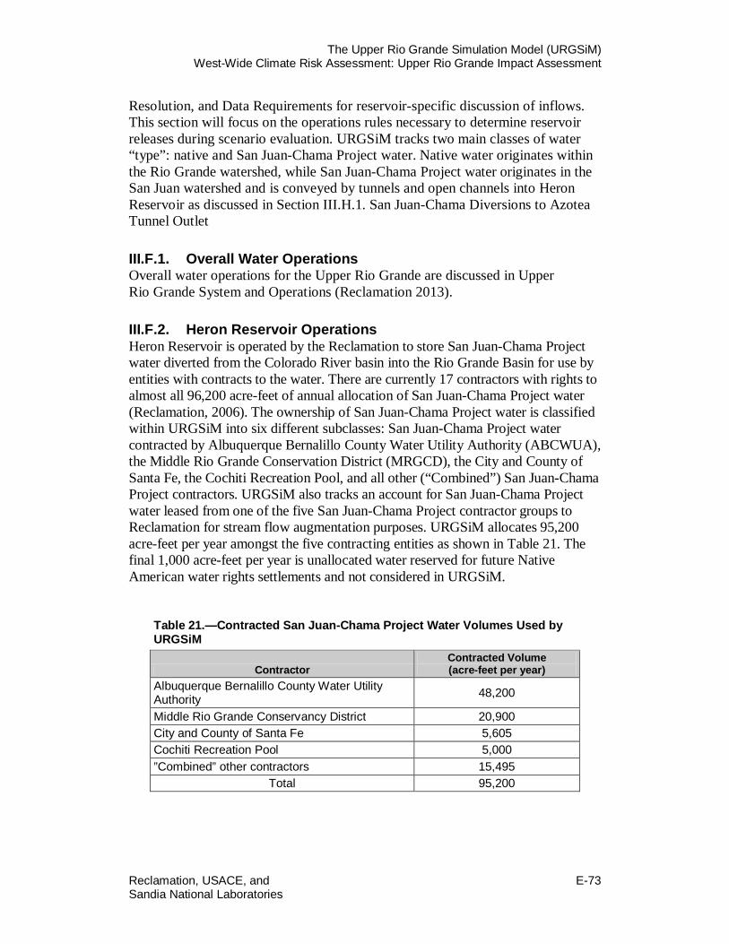
The Upper Rio Grande Simulation Model (URGSiM) West-Wide Climate Risk Assessment: Upper Rio Grande Impact Assessment
Reclamation, USACE, and E-73 Sandia National Laboratories
Resolution, and Data Requirements for reservoir-specific discussion of inflows. This section will focus on the operations rules necessary to determine reservoir releases during scenario evaluation. URGSiM tracks two main classes of water “type”: native and San Juan-Chama Project water. Native water originates within the Rio Grande watershed, while San Juan-Chama Project water originates in the San Juan watershed and is conveyed by tunnels and open channels into Heron Reservoir as discussed in Section III.H.1. San Juan-Chama Diversions to Azotea Tunnel Outlet
III.F.1. Overall Water Operations Overall water operations for the Upper Rio Grande are discussed in Upper Rio Grande System and Operations (Reclamation 2013).
III.F.2. Heron Reservoir Operations Heron Reservoir is operated by the Reclamation to store San Juan-Chama Project water diverted from the Colorado River basin into the Rio Grande Basin for use by entities with contracts to the water. There are currently 17 contractors with rights to almost all 96,200 acre-feet of annual allocation of San Juan-Chama Project water (Reclamation, 2006). The ownership of San Juan-Chama Project water is classified within URGSiM into six different subclasses: San Juan-Chama Project water contracted by Albuquerque Bernalillo County Water Utility Authority (ABCWUA), the Middle Rio Grande Conservation District (MRGCD), the City and County of Santa Fe, the Cochiti Recreation Pool, and all other (“Combined”) San Juan-Chama Project contractors. URGSiM also tracks an account for San Juan-Chama Project water leased from one of the five San Juan-Chama Project contractor groups to Reclamation for stream flow augmentation purposes. URGSiM allocates 95,200 acre-feet per year amongst the five contracting entities as shown in Table 21. The final 1,000 acre-feet per year is unallocated water reserved for future Native American water rights settlements and not considered in URGSiM.
Table 21.—Contracted San Juan-Chama Project Water Volumes Used by URGSiM
Contractor Contracted Volume (acre-feet per year)
Albuquerque Bernalillo County Water Utility Authority 48,200
Middle Rio Grande Conservancy District 20,900 City and County of Santa Fe 5,605 Cochiti Recreation Pool 5,000 ”Combined” other contractors 15,495
Total 95,200
The Upper Rio Grande Simulation Model (URGSiM) West-Wide Climate Risk Assessment: Upper Rio Grande Impact Assessment
E-74 Reclamation, USACE, and
Sandia National Laboratories
In January of each year, the contractor allocation of San Juan-Chama Project water in Heron Reservoir available for use in that year is set to the annual right. Any amount not used by the end of the year reverts to the general pool from which the allocations are reset at the beginning of the next year. In practice, to avoid a dramatic release of unused contractor water from Heron Reservoir at the end of the year, there is some flexibility in release date granted to the contractors to allow releases of the previous year’s water into the next year. In simple terms then, Heron Reservoir is modeled to pass through all native water, and release San Juan-Chama Project water based on modeled requests from contractors up to their annual allocation. The legal framework of San Juan-Chama Project operations mean that evaporative losses are not charged to a given contractor, so the annual allocation of water is available to the contractor at any time in the year. In other reservoirs where the contractors may be allowed to store San Juan-Chama Project water, the water is subject to evaporative losses. The result of this is that contractors are assumed to prefer to leave their allocation of water in Heron Reservoir until they have use for it downstream, only moving it into downstream storage to avoid losing the water to the general pool at the end of the year.
III.F.3. El Vado Reservoir Operations In each timestep, modeled reservoir releases from El Vado Reservoir are determined based on reservoir capacity (determined by the maximum conservation storage elevation), reservoir supply, and downstream demands. Generally, the reservoir is operated to store all native water possible during periods of high inflow in order to serve irrigated areas downstream during periods of lower flow. Operational constraints are associated with Indian lands with irrigation rights, Article VII of the Rio Grande Compact, and San Juan-Chama Project water, each of which is described in greater detail in the following three subsections.
Prior and Paramount Storage The downstream irrigated areas served by El Vado Reservoir include almost 9,000 acres of native American lands with rights that are senior (prior and paramount) to all other irrigation rights. El Vado Reservoir is used to assure water supply through the year to these prior and paramount lands. The amount that should be stored to assure prior and paramount supply is determined by the Bureau of Indian Affairs (BIA), and future development of URGSiM will incorporate the BIA storage requirements. Currently, however, URGSiM uses end of month prior and paramount storage targets shown in Table 22 below. URGSiM classifies each year as dry, average, or wet based on a sum of January through April flows past the Rio Chama near La Puente (USGS 8284100) and Rio Grande at Embudo (USGS 8279500) stream gages compared to the average value for that sum. 80 percent to 120 percent of average flow is defined as an average year, with wet and dry on the outside of that range. While the values shown in Table 22 are different from current BIA requirements, this should have limited impact on the

The Upper Rio Grande Simulation Model (URGSiM) West-Wide Climate Risk Assessment: Upper Rio Grande Impact Assessment
Reclamation, USACE, and E-75 Sandia National Laboratories
Table 22.—End of Month Prior And Paramount Storage Targets Currently Used in URGSiM
Month
El Vado End of Month Prior and Paramount Storage Requirement Used by URGSiM
(acre-feet) Dry Years Average Years Wet Years
January 0 0 0 February 0 0 0
March 0 0 0 April 28,900 8,970 0 May 29,380 9,120 0 June 20,490 6,360 0 July 10,080 3,130 0
August 2,690 830 0 September 0 0 0
October 0 0 0 November 0 0 0 December 0 0 0
effects of increased conservation storage at El Vado Reservoir because prior and paramount storage requirements become important when Article VII is in effect and thus reservoir elevations are low, while an increased reservoir capacity is important when reservoir elevations are high.
Article VII Article VII of the Rio Grande Compact prohibits additions to native storage in El Vado Reservoir if the useable water12 stored in Elephant Butte and Caballo reservoirs is less than 400,000 acre-feet. There are two exceptions to Article VII incorporated into URGSiM:
• Because prior and paramount irrigation rights predate the Rio Grande Compact, native water necessary to assure prior and paramount supply through the growing season can be added to storage in El Vado Reservoir during Article VII restrictions. Thus, native storage up to the amounts shown in Table 22 may be added even during periods of Article VII restrictions. For this reason, prior and paramount native water is tracked separately from MRGCD native water.
12 Useable water in Elephant Butte and Caballo is all native water in the reservoirs, exclusive of any credit water from previous New Mexico or Colorado deliveries in excess of legal requirements.

The Upper Rio Grande Simulation Model (URGSiM) West-Wide Climate Risk Assessment: Upper Rio Grande Impact Assessment
E-76 Reclamation, USACE, and
Sandia National Laboratories
• If New Mexico accrues sufficient compact credits, then by mutual agreement with Texas, some of those credits may be relinquished to be used in the future for storage at El Vado Reservoir (or at other post-compact reservoirs) during periods of Article VII restrictions. MRGCD may use on third of relinquished credits, and Reclamation may use on third by as Reclamation Emergency Drought Water (REDW) for flow augmentation purposes in accordance with the 2003 Emergency Drought Water Agreement.
The MRGCD relinquished credit water becomes native MRGCD water when stored. The REDW is used to meet flow targets between Cochiti and Elephant Butte reservoirs. At each timestep, URGSiM calculates the amount of water required to meet minimum flow targets at Central gage in Albuquerque, Isleta diversion south of Albuquerque, and San Acacia gage. These demands are met with REDW water first, and leased San Juan-Chama Project water stored in Abiquiu Reservoir second. Although not utilized for these runs, URGSiM can be set up to automatically relinquish compact credits once New Mexico credits reach a user defined threshold. These relinquished credits can be used for storage during periods of Article VII restrictions. No relinquishments occurred in the runs evaluated here. Noting that URGSiM includes Elephant Butte and Caballo reservoirs, and thus incorporates Article VII impacts on El Vado Reservoir storage in each time step, is important for an accurate analysis of increased conservation storage opportunities in El Vado Reservoir.
San Juan-Chama Project Accounts In addition to storage of native water for a variety of different uses, El Vado Reservoir is also used in current runs to store San Juan-Chama Project–MRGCD and San Juan-Chama Project–Combined water. Releases of San Juan-Chama Project water from all reservoirs in URGSiM are flagged by ownership and destination, and El Vado Reservoir bypasses any San Juan-Chama Project releases from Heron Reservoir not destined for storage in El Vado Reservoir. San Juan-Chama Project–MRGCD and San Juan-Chama Project–Combined water is moved from Heron Reservoir to El Vado Reservoir when there is storage space available in El Vado Reservoir (up to a static user input maximum allowed volume). In the current URGSiM runs, up to 63,000 acre-feet of San Juan-Chama Project–MRGCD water, and 5,000 acre-feet of San Juan-Chama Project–Combined water can be stored in El Vado Reservoir. San Juan-Chama Project water is moved from El Vado Reservoir to Abiquiu Reservoir if El Vado Reservoir is at or above 75 percent of capacity and there is room for storage of the water in Abiquiu Reservoir.

The Upper Rio Grande Simulation Model (URGSiM) West-Wide Climate Risk Assessment: Upper Rio Grande Impact Assessment
Reclamation, USACE, and E-77 Sandia National Laboratories
Other reservoirs in URGSiM used to store San Juan-Chama Project water besides Heron Reservoir and El Vado Reservoir include Abiquiu Reservoir where San Juan-Chama Project-ABCWUA, San Juan-Chama Project-Combined, and San Juan-Chama Project water leased by Reclamation are stored, and Cochiti Reservoir, where San Juan-Chama Project-Cochiti Recreation Pool water is used to replace evaporative losses to the recreation pool. The San Juan-Chama Project -ABCWUA water is released from Abiquiu Reservoir to pay back groundwater pumping induced river leakage, or for direct diversion in Albuquerque. The groundwater payback portion (also known as “letter” water) used in this model depends on the model scenario being evaluated, and can either be calculated by URGSiM, or be based on external projections. In addition to letter water, San Juan-Chama Project -ABCWUA water is released from Abiquiu Reservoir if available at each timestep up to ½ of ABCWUA total demand, or ½ of the diversion capacity, whichever is smaller. The ½ factor is a result of ABCWUA being allowed to divert an equal amount of native water with the San Juan-Chama Project water, and the native water is then returned to the river as wastewater. Putting this all together, when irrigation demands below Cochiti Reservoir (shown in Table 23) are satisfied by Rio Grande flows, El Vado Reservoir is operated to capture all native inflows that are physically possible and legally allowed in excess of demand. Anything that cannot be physically stored within the defined capacity of the reservoir is passed through. The reservoir capacity for these runs was determined by the maximum conservation storage pool elevations of 6902, 6903, or 6904.22 feet (Project Datum), translated to volumes using the 2007 ACAP tables for El Vado Reservoir. If native Rio Grande flows are not sufficient to cover irrigation demands below Cochiti Reservoir, first native MRGCD water and then San Juan-Chama Project – MRGCD water is released from El Vado Reservoir as available. When that water is gone, MRGCD-owned San Juan-Chama Project water is released directly from Heron Reservoir.
Table 23.—Irrigation Demand (cfs) at Cochiti Reservoir, Including Prior and Paramount Demands
Feb 0 Mar 400 Apr 700 May 900 Jun 925 Jul 925 Aug 900 Sep 700 Oct 550
From URGWOM daily timestep planning model.
In addition to meeting demands below Cochiti Reservoir, URGSiM includes a user specified minimum winter release from El Vado Reservoir of 15 cfs, and the smaller of La Puente inflows or 100 cfs of native water during irrigation season. The summer minimum release is to irrigate approximately 5,000 acres of agricultural lands along the Rio Chama.

The Upper Rio Grande Simulation Model (URGSiM) West-Wide Climate Risk Assessment: Upper Rio Grande Impact Assessment
E-78 Reclamation, USACE, and
Sandia National Laboratories
III.F.4. Abiquiu Reservoir Operations Abiquiu Reservoir is operated by the USACE primarily as a flood control reservoir, though storage of San Juan-Chama Project water, primarily by Albuquerque, has become a significant part of operations. Native water is stored in Abiquiu Reservoir only temporarily to prevent flows downstream from exceeding 1,800 cfs, 3,000 cfs, and 10,000 cfs 1) below the reservoir, 2) at the confluence with the Ojo Caliente, and 3) at the confluence with the Rio Grande respectively. Stored native flood water is released as quickly as possible within the maximum flows listed above, with one exception called carryover storage. To ensure that flood waters that would have been largely unused had they not been stored are not used to supplement irrigation, if flows in the Rio Grande at Otowi are less than 1,500 cfs at any point after July 1 in an irrigation season, then any flood water stored during that irrigation season is delivered downstream after the irrigation season is over. For modeling purposes, native water is not stored except for flood control purposes and is released downstream as soon as possible within the constraints of carryover storage. There is some discussion of native water storage at Abiquiu Reservoir for stream augmentation purposes in the future, and this option is allowed as a user input. The model allows Albuquerque, MRGCD, and the Combined contractor to store 130,000, 2,000, and 11,000 acre-feet respectively in Abiquiu Reservoir based on URGWOM values (Sidlow personal communication 2006). This storage space is used by the contractors as available to avoid losses of allocated water in Heron Reservoir at the beginning of each new year and vacated first by the contractors when there is need for it downstream.
III.F.5. Cochiti Reservoir Operations Cochiti Reservoir, like Abiquiu Reservoir upstream, is operated by the USACE primarily as a flood control reservoir. The only native storage allowed in Cochiti Reservoir is native flood control storage to limit Rio Grande flows between Cochiti and Elephant Butte reservoirs to a maximum of 7,000 cfs. This storage is temporary and evacuated as quickly as possible subject to the same carryover storage requirements described for Abiquiu Reservoir. The only San Juan-Chama Project storage allowed in Cochiti Reservoir is that amount necessary to maintain approximately 1,200 acres of reservoir area for recreation purposes. The 5,000 acre-feet per year San Juan-Chama Project allocation to the Cochiti Recreation Pool is used to offset evaporative losses to the recreation pool in Cochiti Reservoir. Additional storage is disallowed in Cochiti Reservoir in part because large storage volumes in the reservoir lead to high leakage with adverse consequences to agricultural lands downstream of the dam (e.g., Smith 2001).
III.F.6. Jemez Reservoir Operations Jemez Reservoir, like Abiquiu and Cochiti reservoirs, is operated by the USACE primarily for flood control. The reservoir also acts as a sediment barrier to prevent sediment from discharging to the Rio Grande. For model purposes, the only storage allowed in Jemez is native flood control to aid in maintaining Rio Grande

The Upper Rio Grande Simulation Model (URGSiM) West-Wide Climate Risk Assessment: Upper Rio Grande Impact Assessment
Reclamation, USACE, and E-79 Sandia National Laboratories
flows between Cochiti and Elephant Butte reservoirs from exceeding 7,000 cfs. Flood storage in Jemez is subject to the same carryover storage requirements described for Abiquiu Reservoir.
III.F.7. Elephant Butte Reservoir Operations Elephant Butte Reservoir is operated by the Elephant Butte Irrigation District (EBID) to store water delivered from New Mexico to Texas under the requirements of the Rio Grande compact. The water is released for irrigation in southern New Mexico and western Texas. The water released from Elephant Butte Reservoir (and then Caballo Reservoir) is consumed outside of the model boundary according to rules not included in the model. Elephant Butte Reservoir rules are limited to flood control and a target release table. The available water up to the target value is released for each month. Available water includes water in the reservoir less San Juan-Chama Project and New Mexico or Colorado credit water. (Water delivered to Elephant Butte Reservoir from upstream in excess of contract obligation.) URGSiM release targets from Elephant Butte Reservoir by month are shown in Table 24.
Table 24.—Target Releases Used for Elephant Butte and Caballo Reservoirs to Determine Releases in Validation and Scenario Evaluation Modes (Acre-Feet)
Elephant Butte Caballo
January 23,600 7,500
February 52,100 28,100
March 82,700 109,100
April 102,700 89,500
May 122,800 101,800
June 133,000 128,900
July 117,500 135,100
August 81,000 107,400
September 42,100 67,100
October 14,600 15,500
November 6,600 0
December 18,300 0
Total 797,000 790,000
III.F.8. Caballo Reservoir Release Rules Caballo Reservoir, like the larger Elephant Butte Reservoir just upstream, is also operated by EBID. Caballo Reservoir serves largely as additional storage to moderate releases from Elephant Butte Reservoir and adds flexibility to EBID

The Upper Rio Grande Simulation Model (URGSiM) West-Wide Climate Risk Assessment: Upper Rio Grande Impact Assessment
E-80 Reclamation, USACE, and
Sandia National Laboratories
operations. There are no irrigation diversions between Elephant Butte and Caballo reservoirs, and in many ways, Caballo Reservoir is simply an extension of the larger Elephant Butte Reservoir. Release targets used in the model for Caballo Reservoir are shown in Table 24.
III.G. URGSiM Calibration, Validation and Implications on Uncertainty
URGSiM takes surface water inflows at major gage locations, and calculates mass balance based on a historically calibrated representation of reaches and reservoirs. Reaches and reservoirs were calibrated by:
1) Using gaged inflow data (mainstem and tributary) during the historic period, removing gaged or modeled diversions for agriculture if any.
2) Returning gaged or modeled returns from cities and agriculture if any.
3) Adding modeled groundwater additions or reductions.
4) Subtracting direct evaporation in the case of reservoirs adding direct rainfall.
5) Subtracting gaged streamflow at the bottom of the reach, or releases from the reservoir.
The sum of these terms was taken from years 1975 through 1999. If adding water was needed to achieve a 25-year cumulative mass balance, an ungaged surface water inflow term was added as a function of a nearby stream gage. If reducing water was required, calibration was achieved either by:
• Systematic reduction of gaged inflows (Rio Chama at La Puente, Embudo Creek near Dixon, and Rio Puerco near Bernardo)
• Systematic reduction of ungaged inflows (Lobatos to Cerro)
• Increased reservoir leakage (Cochiti Reservoir)
• Decreased carriage water requirements in the conveyance system to increase agricultural consumption (San Acacia to San Marcial)
• Increased riparian ET (San Marcial to Elephant Butte Reservoir) In the case of reservoirs, an error term was added to the reservoir at each calibration timestep to assure that the reservoir storage matched historic data for

The Upper Rio Grande Simulation Model (URGSiM) West-Wide Climate Risk Assessment: Upper Rio Grande Impact Assessment
Reclamation, USACE, and E-81 Sandia National Laboratories
the entire calibration period, and the calibration terms were manipulated until the accumulated error term was zero for the 25-year (1975 through 1999) calibration period. A summary of calibration methods for each reach or reservoir is shown in Table 25. Starting with an analysis of the reliability of the stream gages upon which URGSiM is built, this section provides information on the performance of the model as compared to observed values during the calibration and validation periods.
III.G.1. Observation Uncertainties One way to evaluate model performance is to look at errors, or residuals, at points of historic observation. The points of observation to which we can compare surface water model performance during the calibration period include reservoir storage estimates and stream flows at gages interior to the model and not immediately below a reservoir (the reservoir is calibrated and measured reservoir releases are assumed to be without error). However, the observations themselves are not without error. As documented by the USGS (e.g., Miller and Stiles 2006), the historic observations of stream flow contain errors and uncertainties from two main sources:
• The stability of the stag flow relationship at the gage location. The gage measures stream stage and uses a relationship between stage and flow, derived from field measurements of flow at various stages, to estimate stream flow. However, this relationship can change as the stream bed changes due to sediment or vegetation build up.
• The accuracy of the direct measurement of the flow rate. Direct measurement of stream flow is done with velocity and depth measurements, and a myriad of assumptions as to the velocity profile through the two dimensional profile through which flow occurs (e.g., Carter and Davidian 1968).
Similarly, the historic estimates of reservoir storage contain errors associated with:
• The stability and accuracy of the stag storage relationship of the reservoir. This stag storage relationship is estimated based on topographic surveys and changes as sediment builds up in the reservoir.

The Upper Rio Grande Simulation Model (URGSiM) West-Wide Climate Risk Assessment: Upper Rio Grande Impact Assessment
E-82 Reclamation, USACE, and
Sandia National Laboratories
Table 25.—Surface Water Calibration Methods and Magnitude of the Calibration Term for URGSiM Reaches and Reservoirs
Reach or Reservoir Calibration Term Gage Used Factor Used
Average Magnitude 1975-1999
(cfs) Chama: SJC Diversions to Azotea none none none 0 Chama: Willow Creek to below Heron Ungaged SW inflow Chama near La Puente 6.8% summer only 26 Chama: Below Heron to below El Vado Gaged SW reduction Chama near La Puente 35% of flow > 2000 cfs -17 Chama: Below El Vado to Abiquiu Ungaged SW inflow Ojo Caliente near La Madera 35% summer only 25 Abiquiu Reservoir Ungaged SW inflow Jemez River near Jemez 54% 48 Chama: Below Abiquiu Res. to Chamita Ungaged SW inflow Ojo Caliente near La Madera 3.5% summer only 3 Colorado Index Gages to Lobatos none none none 0 Lobatos to Cerro Ungaged GW reduction none 38 instead of 39cfs -1 Cerro to Taos Junction Bridge Ungaged SW inflow Rio P. de Taos below Los Cordovas 62% summer only 42 Taos Junction Bridge to Embudo Gaged SW reduction Embudo Creek near Dixon 23% of flow > 200 cfs -7 Embudo to Otowi Ungaged SW inflow Rio Nambe below Reservoir 47cfs base + 120% summer gage 63 Otowi to below Cochiti Reservoir Reservoir leakage NA none -31 Below Cochiti Reservoir to San Felipe Ungaged SW inflow Galisteo Creek below Galisteo Dam 156% 9 Jemez: Jemez Pueblo to below Reservoir Ungaged SW inflow Jemez River near Jemez 52% of flows up to 200 cfs only 36 San Felipe to Albuquerque Ungaged SW inflow N Floodway Channel near Alameda 92% 36 Albuquerque to Bernardo Ungaged SW inflow Tijeras Arroyo & S Div Channel 165% 2.5 Bernardo to San Acacia Gaged SW reduction Rio Puerco near Bernardo 36% reduction -12 San Acacia to San Marcial Carriage Water none 11% instead of 15% NA San Marcial to below Elephant Butte Riparian ET none none NA Below Elephant Butte to below Caballo Ungaged SW inflow Caballo Reservoir Precipitation Caballo Res Precip * 26,000 acres 34 SJC is San Juan-Chama Project

The Upper Rio Grande Simulation Model (URGSiM) West-Wide Climate Risk Assessment: Upper Rio Grande Impact Assessment
Reclamation, USACE, and E-83 Sandia National Laboratories
• The accuracy of the measurement of stage in the reservoir. This is presumably a relatively easy measurement that can be done quite accurately; however, it is a point measurement that is assumed to represent the entire reservoir, and the sensitivity of the volume estimate to small changes in stage is significant.
Ideally, the model residuals during calibration will be normally distributed about zero and be comparable to the distribution of uncertainty associated with the observations themselves, which should also be distributed normally about zero. The accuracy of the stream gages will be evaluated here from two perspectives:
• According to USGS ratings of the gages, The USGS, in its annual water data reports (e.g., Miller and Stiles 2006), rates each gage during a given water year as excellent, good, fair, or poor when 95 percent of gage estimates are thought to be within 5 percent, 10 percent, 15 percent, or more than 15 percent of the true value respectively. If we assume that when a gage is rated as poor, 95 percent of the gage estimates are within 50 percent of the true value, we can assign quantitative 95 percent confidence intervals to the calibration gages in the model during the 1975 through 1999 historic period. Based on the USGS ratings, the best gage during the calibration period is the Rio Grande gage below Taos Junction Bridge (Table 3) which was predicted to have been within 9 percent of the actual stream flow 95 percent of the time between 1975 and 1999. The worst gage was the Rio Grande Floodway gage near San Acacia (Table 3), which was estimated to be within only 36 percent of the actual stream flow 95 percent of the time. Values for calibration gages are shown in Table 26, along with values estimated based on field based flow measurements as described below.
The distribution of uncertainty associated with stream gages can also be inferred by comparing stag based flow estimates to velocity-area-based flow estimates used to calibrate the stag flow relationship at a given gage. (A similar approach could be used for reservoir storage estimates by comparing the stage based estimate to a more direct measurement using gravity changes for example; however, the author is not aware of any such direct measurements associated with the reservoirs within the model extent.) Initial gage error distribution estimates were developed for the 1975 through 1999 period by plotting stage versus measured flow for all field measurements at the calibration gage locations from 1975 through 1999. Error was assumed to be equal to the difference between the measured values and a single best fit rating curve. This method led to
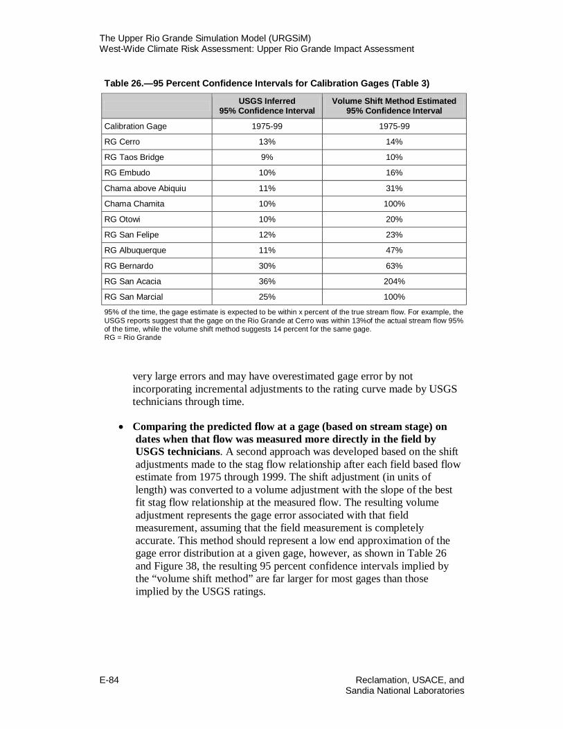
The Upper Rio Grande Simulation Model (URGSiM) West-Wide Climate Risk Assessment: Upper Rio Grande Impact Assessment
E-84 Reclamation, USACE, and
Sandia National Laboratories
Table 26.—95 Percent Confidence Intervals for Calibration Gages (Table 3)
USGS Inferred 95% Confidence Interval
Volume Shift Method Estimated 95% Confidence Interval
Calibration Gage 1975-99 1975-99
RG Cerro 13% 14%
RG Taos Bridge 9% 10%
RG Embudo 10% 16%
Chama above Abiquiu 11% 31%
Chama Chamita 10% 100%
RG Otowi 10% 20%
RG San Felipe 12% 23%
RG Albuquerque 11% 47%
RG Bernardo 30% 63%
RG San Acacia 36% 204%
RG San Marcial 25% 100%
95% of the time, the gage estimate is expected to be within x percent of the true stream flow. For example, the USGS reports suggest that the gage on the Rio Grande at Cerro was within 13%of the actual stream flow 95% of the time, while the volume shift method suggests 14 percent for the same gage. RG = Rio Grande
very large errors and may have overestimated gage error by not incorporating incremental adjustments to the rating curve made by USGS technicians through time.
• Comparing the predicted flow at a gage (based on stream stage) on dates when that flow was measured more directly in the field by USGS technicians. A second approach was developed based on the shift adjustments made to the stag flow relationship after each field based flow estimate from 1975 through 1999. The shift adjustment (in units of length) was converted to a volume adjustment with the slope of the best fit stag flow relationship at the measured flow. The resulting volume adjustment represents the gage error associated with that field measurement, assuming that the field measurement is completely accurate. This method should represent a low end approximation of the gage error distribution at a given gage, however, as shown in Table 26 and Figure 38, the resulting 95 percent confidence intervals implied by the “volume shift method” are far larger for most gages than those implied by the USGS ratings.

The Upper Rio Grande Simulation Model (URGSiM) West-Wide Climate Risk Assessment: Upper Rio Grande Impact Assessment
Reclamation, USACE, and E-85 Sandia National Laboratories
Figure 38.—Stage and discharge relationships based on 1975-1999 field measurement at gage locations along the Rio Grande near Cerro and Albuquerque (It is clear that the Albuquerque gage has a less stable relationship between stage and discharge through time than the Cerro gage, and thus is presumably less reliable. The volume shift adjustment method of gage uncertainty predicts this difference, while the USGS gage ratings do not (Table 26). The two methods agree very well for the gages at Cerro and Taos Bridge but are disparate for most of the other gage locations. If we again consider (as discussed above) that the uncertainty is a function of the stability of the flow stage relationship and the accuracy of direct measurement, and we assume that the direct measurement accuracy is similar for all stream locations within the model, then it is difficult to believe, as suggested by the USGS inferred ratings, that the gage on the Rio Grande at Albuquerque, a sometimes braided river channel characterized by a sandy, moving bed can be more accurate than the gage at Cerro. Figure 39 shows flow versus stage relationships for field measurements at each gage between 1975 and 1999 to reinforce this point. It seems that the volume shift adjustment method may provide more reliable (though less optimistic) estimates of gage reliability.
Stage to discharge relationships along the Rio Grande near Cerro and at Albuquerque measured between 1975 and 1999
-
2.00
4.00
6.00
8.00
10.00
12.00
14.00
- 1,000 2,000 3,000 4,000 5,000 6,000 7,000 8,000
Stream discharge [cfs]
Stre
am s
tage
[ft]
AlbuquerqueCerro

The Upper Rio Grande Simulation Model (URGSiM) West-Wide Climate Risk Assessment: Upper Rio Grande Impact Assessment
E-86 Reclamation, USACE, and
Sandia National Laboratories
Figure 39.—Accuracy range of a given gage 1975-99 as a function of the percentage of readings within that range (volume adjust method). The better a gage, the further left it will plot on this figure. According to USGS ratings, the gage below Taos Junction Bridge, and near Cerro, would rate as “good” and “fair” respectively, while all other gages would rate as “poor”. With the exception of the gage below Taos Junction Bridge, and near Cerro, which rate as “good” and “fair” respectively, all of the gages in Table 26 merit USGS “poor” ratings for 1975 through 1999 based on the volume shift adjustment method. This result is shown graphically in Figure 39. The USGS gage network is an impressive resource that is invaluable to hydrologic science, and this study (among others) would not have been possible without it. The quantitative meaning associated with the USGS ratings of their gages may be infrequently scrutinized or relied upon in other calculations, but the estimates of gage uncertainty published by the USGS seem optimistic. In their defense, to consider estimates of discharge on a variable and sediment dominated stream as “poor” if they are not within 15 percent of the actual value 95 percent of the time may not be realistic.
III.G.2. Calibration Residuals The distribution of calibration residuals (historic observation less model value) for URGSiM modeled flows at gaged locations within the model extent (Table 3) for each month from 1975 through 1999 are shown in Figure 40 through Figure 50. In
Gage uncertainty 1975-99 for calibration gages based on the volume adjust method, with USGS ratings scale included.
50%
55%
60%
65%
70%
75%
80%
85%
90%
95%
100%
0% 5% 10% 15% 20%
Accuracy Range [+ or -]
% o
f gag
e re
adin
gs e
xpec
ted
to b
e w
ithin
ac
cura
cy ra
nge
of tr
ue v
alue
C aAbC CtaRG CroRG TBRG EmbRG OtwRG SFpRG AlbRG BdoRG SARG SM
USGS Excellent USGS Good USGS Fair
USGS Poor

The Upper Rio Grande Simulation Model (URGSiM) West-Wide Climate Risk Assessment: Upper Rio Grande Impact Assessment
Reclamation, USACE, and E-87 Sandia National Laboratories
Figure 40.—Model residual (observed – modeled) distribution for the surface water gage on the Chama above Abiquiu Reservoir (USGS Gage ID 8286500) for the 1975 through 1999 calibration period. Ideally, modeled residuals are normally distributed tightly about zero.
Figure 41.—Model residual (observed – modeled) distribution for the surface water gage on the Chama near Chamita (USGS Gage ID 8290000) for the 1975 through 1999 calibration period.
Rio Chama above Abiquiu
0%
5%
10%
15%
20%
25%
30%
35%
< -5
00
-500
to -4
00
-400
to -3
00
-300
to -2
00
-200
to -1
80
-180
to -1
60
-160
to -1
40
-140
to -1
20
-120
to -1
00
-100
to -8
0
-80
to -6
0
-60
to -4
0
-40
to -2
0
-20
to 0
0 to
20
20
to 4
0
40
to 6
0
60
to 8
0
80
to 1
00
100
to 1
20
120
to 1
40
140
to 1
60
160
to 1
80
180
to 2
00
200
to 3
00
300
to 4
00
400
to 5
00
> 50
0
Model Calibration Residual (observed - modeled flow at gage) [cfs]
Prob
abili
ty
Rio Chama near Chamita
0%
5%
10%
15%
20%
25%
30%
< -5
00
-500
to -4
00
-400
to -3
00
-300
to -2
00
-200
to -1
80
-180
to -1
60
-160
to -1
40
-140
to -1
20
-120
to -1
00
-100
to -8
0
-80
to -6
0
-60
to -4
0
-40
to -2
0
-20
to 0
0 to
20
20
to 4
0
40
to 6
0
60
to 8
0
80
to 1
00
100
to 1
20
120
to 1
40
140
to 1
60
160
to 1
80
180
to 2
00
200
to 3
00
300
to 4
00
400
to 5
00
> 50
0
Model Calibration Residual (observed - modeled flow at gage) [cfs]
Prob
abili
ty1975-1999 annual average flow: 550 cfs
1975-1999 annual average flow: 640 cfs

The Upper Rio Grande Simulation Model (URGSiM) West-Wide Climate Risk Assessment: Upper Rio Grande Impact Assessment
E-88 Reclamation, USACE, and
Sandia National Laboratories
Figure 42.—Model residual (observed – modeled) distribution for the surface water gage on the Rio Grande near Cerro (USGS Gage ID 8263500) for the 1975 through1999 calibration period.
Figure 43.—Model residual (observed – modeled) distribution for the surface water gage on the Rio Grande below Taos Bridge (USGS Gage ID 8276500) for the 1975 through 1999 calibration period.
Rio Grande near Cerro
0%
5%
10%
15%
20%
25%
30%
35%
< -5
00
-500
to -4
00
-400
to -3
00
-300
to -2
00
-200
to -1
80
-180
to -1
60
-160
to -1
40
-140
to -1
20
-120
to -1
00
-100
to -8
0
-80
to -6
0
-60
to -4
0
-40
to -2
0
-20
to 0
0 to
20
20
to 4
0
40
to 6
0
60
to 8
0
80
to 1
00
100
to 1
20
120
to 1
40
140
to 1
60
160
to 1
80
180
to 2
00
200
to 3
00
300
to 4
00
400
to 5
00
> 50
0
Model Calibration Residual (observed - modeled flow at gage) [cfs]
Prob
abili
ty
Rio Grande Below Taos Bridge
0%
5%
10%
15%
20%
25%
30%
35%
< -5
00
-500
to -4
00
-400
to -3
00
-300
to -2
00
-200
to -1
80
-180
to -1
60
-160
to -1
40
-140
to -1
20
-120
to -1
00
-100
to -8
0
-80
to -6
0
-60
to -4
0
-40
to -2
0
-20
to 0
0 to
20
20
to 4
0
40
to 6
0
60
to 8
0
80
to 1
00
100
to 1
20
120
to 1
40
140
to 1
60
160
to 1
80
180
to 2
00
200
to 3
00
300
to 4
00
400
to 5
00
> 50
0
Model Calibration Residual (observed - modeled flow at gage) [cfs]
Prob
abili
ty1975-1999 annual average flow: 580 cfs
1975-1999 annual average flow: 850 cfs

The Upper Rio Grande Simulation Model (URGSiM) West-Wide Climate Risk Assessment: Upper Rio Grande Impact Assessment
Reclamation, USACE, and E-89 Sandia National Laboratories
Figure 44.—Model residual (observed – modeled) distribution for the surface water gage on the Rio Grande at Embudo (USGS Gage ID 8279500) for the 1975 through1999 calibration period.
Figure 45.—Model residual (observed – modeled) distribution for the surface water gage on the Rio Grande at Otowi (USGS Gage ID 8313000) for the 1975 through 1999 calibration period.
Rio Grande at Embudo
0%
5%
10%
15%
20%
25%
30%
35%
40%
< -5
00
-500
to -4
00
-400
to -3
00
-300
to -2
00
-200
to -1
80
-180
to -1
60
-160
to -1
40
-140
to -1
20
-120
to -1
00
-100
to -8
0
-80
to -6
0
-60
to -4
0
-40
to -2
0
-20
to 0
0 to
20
20
to 4
0
40
to 6
0
60
to 8
0
80
to 1
00
100
to 1
20
120
to 1
40
140
to 1
60
160
to 1
80
180
to 2
00
200
to 3
00
300
to 4
00
400
to 5
00
> 50
0
Model Calibration Residual (observed - modeled flow at gage) [cfs]
Prob
abili
ty
Rio Grande at Otowi
0%
5%
10%
15%
20%
< -5
00
-500
to -4
00
-400
to -3
00
-300
to -2
00
-200
to -1
80
-180
to -1
60
-160
to -1
40
-140
to -1
20
-120
to -1
00
-100
to -8
0
-80
to -6
0
-60
to -4
0
-40
to -2
0
-20
to 0
0 to
20
20
to 4
0
40
to 6
0
60
to 8
0
80
to 1
00
100
to 1
20
120
to 1
40
140
to 1
60
160
to 1
80
180
to 2
00
200
to 3
00
300
to 4
00
400
to 5
00
> 50
0
Model Calibration Residual (observed - modeled flow at gage) [cfs]
Prob
abili
ty1975-1999 annual average flow: 950 cfs
1975-1999 annual average flow: 1,660 cfs

The Upper Rio Grande Simulation Model (URGSiM) West-Wide Climate Risk Assessment: Upper Rio Grande Impact Assessment
E-90 Reclamation, USACE, and
Sandia National Laboratories
Figure 46.—Model residual (observed – modeled) distribution for the surface water gage on the Rio Grande at San Felipe (USGS Gage ID 8319000) for the 1975 through 1999 calibration period.
Figure 47.—Model residual (observed – modeled) distribution for the surface water gage on the Rio Grande at Central Avenue in Albuquerque (USGS Gage ID 8330000) for the 1975 through 1999 calibration period.
Rio Grande at San Felipe
0%
2%
4%
6%
8%
10%
12%
14%
< -5
00 -5
00 to
-400
-400
to -3
00 -3
00 to
-200
-200
to -1
80 -1
80 to
-160
-160
to -1
40 -1
40 to
-120
-120
to -1
00 -1
00 to
-80
-80
to -6
0 -6
0 to
-40
-40
to -2
0 -2
0 to
0
0 to
20
20
to 4
0 4
0 to
60
60
to 8
0 8
0 to
100
100
to 1
2012
0 to
140
140
to 1
6016
0 to
180
180
to 2
0020
0 to
300
300
to 4
0040
0 to
500
> 50
0
Model Calibration Residual (observed - modeled flow at gage) [cfs]
Prob
abili
ty
Rio Grande at Central
0%
2%
4%
6%
8%
10%
< -5
00 -5
00 to
-400
-400
to -3
00 -3
00 to
-200
-200
to -1
80 -1
80 to
-160
-160
to -1
40 -1
40 to
-120
-120
to -1
00 -1
00 to
-80
-80
to -6
0 -6
0 to
-40
-40
to -2
0 -2
0 to
0 0
to 2
0 2
0 to
40
40
to 6
0 6
0 to
80
80
to 1
0010
0 to
120
120
to 1
4014
0 to
160
160
to 1
8018
0 to
200
200
to 3
0030
0 to
400
400
to 5
00>
500
Model Calibration Residual (observed - modeled flow at gage) [cfs]
Prob
abili
ty1975-1999 annual average flow: 1,610 cfs
1975-1999 annual average flow: 1,480 cfs

The Upper Rio Grande Simulation Model (URGSiM) West-Wide Climate Risk Assessment: Upper Rio Grande Impact Assessment
Reclamation, USACE, and E-91 Sandia National Laboratories
Figure 48.—Model residual (observed – modeled) distribution for the surface water gage on the Rio Grande floodway at Bernardo (USGS Gage ID 8332010) for the 1975 through 1999 calibration period.
Figure 49.—Model residual (observed – modeled) distribution for the surface water gage on the Rio Grande floodway at San Acacia (USGS Gage ID 8354900) for the 1975 through 1999 calibration period.
Rio Grande at Bernardo
0%
2%
4%
6%
8%
10%
< -5
00 -5
00 to
-400
-400
to -3
00 -3
00 to
-200
-200
to -1
80 -1
80 to
-160
-160
to -1
40 -1
40 to
-120
-120
to -1
00 -1
00 to
-80
-80
to -6
0 -6
0 to
-40
-40
to -2
0 -2
0 to
0 0
to 2
0 2
0 to
40
40
to 6
0 6
0 to
80
80
to 1
0010
0 to
120
120
to 1
4014
0 to
160
160
to 1
8018
0 to
200
200
to 3
0030
0 to
400
400
to 5
00>
500
Model Calibration Residual (observed - modeled flow at gage) [cfs]
Prob
abili
ty
Rio Grande at San Acacia
0%
2%
4%
6%
8%
10%
12%
< -5
00 -5
00 to
-400
-400
to -3
00 -3
00 to
-200
-200
to -1
80 -1
80 to
-160
-160
to -1
40 -1
40 to
-120
-120
to -1
00 -1
00 to
-80
-80
to -6
0 -6
0 to
-40
-40
to -2
0 -2
0 to
0 0
to 2
0 2
0 to
40
40
to 6
0 6
0 to
80
80
to 1
0010
0 to
120
120
to 1
4014
0 to
160
160
to 1
8018
0 to
200
200
to 3
0030
0 to
400
400
to 5
00>
500
Model Calibration Residual (observed - modeled flow at gage) [cfs]
Prob
abili
ty1975-1999 annual average flow: 1,320 cfs
1975-1999 annual average flow: 1160 cfs

The Upper Rio Grande Simulation Model (URGSiM) West-Wide Climate Risk Assessment: Upper Rio Grande Impact Assessment
E-92 Reclamation, USACE, and
Sandia National Laboratories
Figure 50.—Model residual (observed – modeled) distribution for the surface water gage on the Rio Grande floodway at San Marcial (USGS Gage ID 8358400) for the 1975 through 1999 calibration period. general, model performance degrades as distance downstream increases. This is a combination of increases in system complexity with distance downstream, and the decreases in gage accuracy seen in Table 26 and Figure 39 that result from shifting channel geometries associated with sand-dominated riverbeds characteristic of lower reaches. Storage residuals for the seven reservoirs within the model extent for the same time period are shown in Figure 51 through Figure 57. Figure 58 shows the cumulative distribution of the reservoir residuals, and shows clearly that Elephant Butte Reservoir residuals are the largest, and Jemez residuals the smallest. Figure 59 shows the cumulative distribution of the reservoir residuals normalized to the capacity of each reservoir. Caballo Reservoir is the most poorly modeled reservoir from a percent of capacity perspective, while the other reservoirs are tightly clustered. Abiquiu Reservoir residuals are small as a percent of capacity, due to a large—but typically unused— capacity.
Rio Grande at San Marcial
0%
2%
4%
6%
8%
10%
12%
< -5
00 -5
00 to
-400
-400
to -3
00 -3
00 to
-200
-200
to -1
80 -1
80 to
-160
-160
to -1
40 -1
40 to
-120
-120
to -1
00 -1
00 to
-80
-80
to -6
0 -6
0 to
-40
-40
to -2
0 -2
0 to
0 0
to 2
0 2
0 to
40
40
to 6
0 6
0 to
80
80
to 1
0010
0 to
120
120
to 1
4014
0 to
160
160
to 1
8018
0 to
200
200
to 3
0030
0 to
400
400
to 5
00>
500
Model Calibration Residual (observed - modeled flow at gage) [cfs]
Prob
abili
ty1975-1999 annual average flow: 1080 cfs
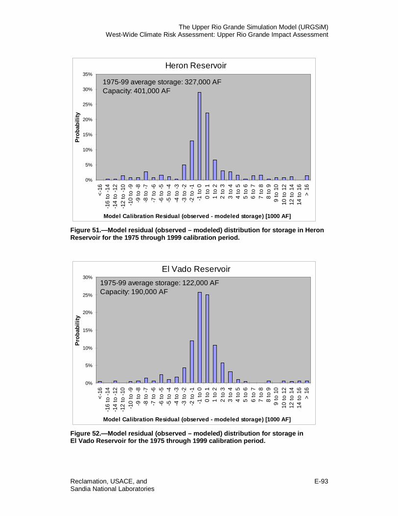
The Upper Rio Grande Simulation Model (URGSiM) West-Wide Climate Risk Assessment: Upper Rio Grande Impact Assessment
Reclamation, USACE, and E-93 Sandia National Laboratories
Figure 51.—Model residual (observed – modeled) distribution for storage in Heron Reservoir for the 1975 through 1999 calibration period.
Figure 52.—Model residual (observed – modeled) distribution for storage in El Vado Reservoir for the 1975 through 1999 calibration period.
Heron Reservoir
0%
5%
10%
15%
20%
25%
30%
35%
<-16
-16
to -1
4 -1
4 to
-12
-12
to -1
0 -1
0 to
-9 -9
to -8
-8 to
-7 -7
to -6
-6 to
-5 -5
to -4
-4 to
-3 -3
to -2
-2 to
-1 -1
to 0
0 to
11
to 2
2 to
33
to 4
4 to
55
to 6
6 to
77
to 8
8 to
99
to 1
010
to 1
212
to 1
414
to 1
6>
16
Model Calibration Residual (observed - modeled storage) [1000 AF]
Prob
abili
ty1975-99 average storage: 327,000 AFCapacity: 401,000 AF
El Vado Reservoir
0%
5%
10%
15%
20%
25%
30%
<-16
-16
to -1
4 -1
4 to
-12
-12
to -1
0 -1
0 to
-9 -9
to -8
-8 to
-7 -7
to -6
-6 to
-5 -5
to -4
-4 to
-3 -3
to -2
-2 to
-1 -1
to 0
0 to
11
to 2
2 to
33
to 4
4 to
55
to 6
6 to
77
to 8
8 to
99
to 1
010
to 1
212
to 1
414
to 1
6>
16
Model Calibration Residual (observed - modeled storage) [1000 AF]
Prob
abili
ty
1975-99 average storage: 122,000 AFCapacity: 190,000 AF
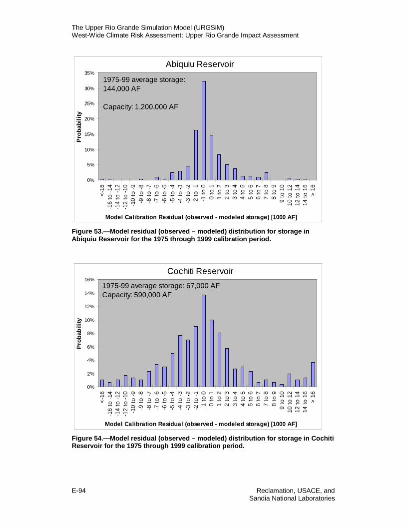
The Upper Rio Grande Simulation Model (URGSiM) West-Wide Climate Risk Assessment: Upper Rio Grande Impact Assessment
E-94 Reclamation, USACE, and
Sandia National Laboratories
Figure 53.—Model residual (observed – modeled) distribution for storage in Abiquiu Reservoir for the 1975 through 1999 calibration period.
Figure 54.—Model residual (observed – modeled) distribution for storage in Cochiti Reservoir for the 1975 through 1999 calibration period.
Abiquiu Reservoir
0%
5%
10%
15%
20%
25%
30%
35%
<-16
-16
to -1
4 -1
4 to
-12
-12
to -1
0 -1
0 to
-9 -9
to -8
-8 to
-7 -7
to -6
-6 to
-5 -5
to -4
-4 to
-3 -3
to -2
-2 to
-1 -1
to 0
0 to
11
to 2
2 to
33
to 4
4 to
55
to 6
6 to
77
to 8
8 to
99
to 1
010
to 1
212
to 1
414
to 1
6>
16
Model Calibration Residual (observed - modeled storage) [1000 AF]
Prob
abili
ty1975-99 average storage:144,000 AF
Capacity: 1,200,000 AF
Cochiti Reservoir
0%
2%
4%
6%
8%
10%
12%
14%
16%
<-16
-16
to -1
4 -1
4 to
-12
-12
to -1
0 -1
0 to
-9 -9
to -8
-8 to
-7 -7
to -6
-6 to
-5 -5
to -4
-4 to
-3 -3
to -2
-2 to
-1 -1
to 0
0 to
11
to 2
2 to
33
to 4
4 to
55
to 6
6 to
77
to 8
8 to
99
to 1
010
to 1
212
to 1
414
to 1
6>
16
Model Calibration Residual (observed - modeled storage) [1000 AF]
Prob
abili
ty
1975-99 average storage: 67,000 AFCapacity: 590,000 AF

The Upper Rio Grande Simulation Model (URGSiM) West-Wide Climate Risk Assessment: Upper Rio Grande Impact Assessment
Reclamation, USACE, and E-95 Sandia National Laboratories
Figure 55.—Model residual (observed – modeled) distribution for storage in Jemez Reservoir for the 1975 through 1999 calibration period.
Figure 56.—Model residual (observed – modeled) distribution for storage in Elephant Butte Reservoir for the 1975 through 1999 calibration period. Elephant Butte Reservoir is a significantly larger reservoir than other modeled reservoirs, thus the different bin ranges (x-axis). Ideally, modeled residuals are normally distributed tightly about zero.
Jemez Reservoir
0%
5%
10%
15%
20%
25%
30%
35%
<-16
-16
to -1
4 -1
4 to
-12
-12
to -1
0 -1
0 to
-9 -9
to -8
-8 to
-7 -7
to -6
-6 to
-5 -5
to -4
-4 to
-3 -3
to -2
-2 to
-1 -1
to 0
0 to
11
to 2
2 to
33
to 4
4 to
55
to 6
6 to
77
to 8
8 to
99
to 1
010
to 1
212
to 1
414
to 1
6>
16
Model Calibration Residual (observed - modeled storage) [1000 AF]
Prob
abili
ty1975-99 average storage:16,000 AF
Capacity: 260,000 AF
Elephant Butte Reservoir
0%
2%
4%
6%
8%
10%
12%
14%
<32.
5 -3
2.5
to 3
0 -3
0 to
-27.
5 -2
7.5
to 2
5 -2
5 to
22.
5 -2
2.5
to 2
0 -2
0 to
-17.
5 -1
7.5
to 1
5 -1
5 to
12.
5 -1
2.5
to -1
0 -1
0 to
-7.5
-7.5
to -5
-5 to
-2.5
-2.5
to 0
0 to
2.5
2.5
to 5
5 to
7.5
7.5
to 1
010
to 1
2.5
12.5
to 1
515
to 1
7.5
17.5
to 2
020
to 2
2.5
22.5
to 2
525
to 2
7.5
27.5
to 3
030
to 3
2.5
>32.
5
Model Calibration Residual (observed - modeled storage) [1000 AF]
Prob
abili
ty
1975-99 average storage: 1,390,000 AFCapacity: 2,023,000 AF

The Upper Rio Grande Simulation Model (URGSiM) West-Wide Climate Risk Assessment: Upper Rio Grande Impact Assessment
E-96 Reclamation, USACE, and
Sandia National Laboratories
Figure 57.—Model residual (observed – modeled) distribution for storage in Caballo Reservoir during 1975 through 1999 calibration period.
Figure 58.—Cumulative distribution of monthly reservoir storage residuals shown in Figure 51 through Figure 57. The graph shows the percent of monthly storage residuals (y-axis) whose absolute value is within a given volume (x-axis).
Caballo Reservoir
0%
2%
4%
6%
8%
10%
12%
14%
<-16
-16
to -1
4 -1
4 to
-12
-12
to -1
0 -1
0 to
-9 -9
to -8
-8 to
-7 -7
to -6
-6 to
-5 -5
to -4
-4 to
-3 -3
to -2
-2 to
-1 -1
to 0
0 to
11
to 2
2 to
33
to 4
4 to
55
to 6
6 to
77
to 8
8 to
99
to 1
010
to 1
212
to 1
414
to 1
6>
16
Model Calibration Residual (observed - modeled storage) [1000 AF]
Prob
abili
ty1975-99 average storage: 99,000 AFCapacity: 328,000 AF
Cumulative distribution of monthly reservoir storage residuals
0%
25%
50%
75%
100%
0 5 10 15 20 25 30 351000 AF
Perc
ent o
f res
idua
ls w
ithin
giv
en v
olum
e
HeronEl VadoAbiquiuCochitiJemezElephant ButteCaballo

The Upper Rio Grande Simulation Model (URGSiM) West-Wide Climate Risk Assessment: Upper Rio Grande Impact Assessment
Reclamation, USACE, and E-97 Sandia National Laboratories
Figure 59.—Cumulative distribution of monthly reservoir storage residuals normalized to reservoir capacity. The graph shows the percent of monthly storage residuals (y-axis) whose absolute value is within a given percent of the individual reservoir capacity (x-axis).
III.G.3. Validation Residual Analysis for Stream Flow Observations After the 1975 through 1999 calibration period, the model is run in validation mode from 2000 through 200413. In validation mode, input gages (river reaches begin either at an input gage for headwater reaches or at a calibration gage marking the end of the reach above). Input gages are listed in Table 2, and calibration gages in Table 3. Input gages are located on the model boundary and provide inflows to the top of headwater reaches as well as tributary inflows to reaches throughout the system. Calibration gages are stream gages at the end of river reaches that are internal to the model extent and that have continuous historic records (starting no later than 1975). At the calibration gages, modeled values can be compared to observed values during the historic period. Climate data are fed with historic observations. Irrigated and riparian acreages are set to 1999 values. River diversions upstream of Cochiti Reservoir are set to twice modeled agricultural ET demand, with half of the diversion returning to the river. River diversions downstream of Cochiti Reservoir are set to monthly average values from 1975 through 1999 up to the amount of water available, and reservoir releases are based on either historic observations or rules, depending on the analysis. Validation results presented first are for historic reservoir releases. 13 This analysis was done in 2006. URGSiM is now (as of 2013) run in validation mode through 2009. An updated validation analysis is overdue.
Cumulative distribution of monthly reservoir residuals expressed as a percentage of reservoir capacity
0%
25%
50%
75%
100%
0.0% 0.5% 1.0% 1.5% 2.0% 2.5% 3.0% 3.5%
Percent of reservoir capacity
Perc
ent o
f res
idua
ls w
ithin
a g
iven
pe
rcen
tage
of r
eser
voir
capa
city
HeronEl VadoAbiquiuCochitiJemezEBCaballo

The Upper Rio Grande Simulation Model (URGSiM) West-Wide Climate Risk Assessment: Upper Rio Grande Impact Assessment
E-98 Reclamation, USACE, and
Sandia National Laboratories
Validation residuals are the observed – modeled values at internal observation points during the 2000 through 2004 period. As shown in Figure 60, hydrologic conditions during the 2000 through 2004 validation period were significantly drier than those of the 1975 through 1999 calibration period. In fact, total flow at Otowi during the five years used for validation was less than for any five year period from 1975 through 2004, suggesting this is not a representative validation period. This may lead to worse model performance during the validation period than might be expected from a more average series of years.
Figure 60.—Gaged annual flows at Otowi bridge 1975 through 2004. Figure 61 compares estimated gage uncertainty with calibration and validation residuals (historic observation value less modeled value). Four important results can be drawn from Figure 61:
• For most gage locations, the estimated gage uncertainty (left-most bar) is comparable to the calibration residuals (middle bar). This suggests, that for the reaches above these gages the model is limited most significantly by the quality of the historic observations (during calibration, the flows at interior gages (Table 3) are reset to match historic observations).
Annual Flow Recorded at Otowi Gage 1975-2004
0
500000
1000000
1500000
2000000
2500000
1975 1980 1985 1990 1995 2000 2005
Year
Otow
i Flo
w [A
F/yr
]
Otow i recorded f low
5 year moving average
Validation Period

The Upper Rio Grande Simulation Model (URGSiM) West-Wide Climate Risk Assessment: Upper Rio Grande Impact Assessment
Reclamation, USACE, and E-99 Sandia National Laboratories
Figure 61.—Comparison of expected gage accuracy (left bar) to calibration and validation residuals (observed – modeled) for calibration gages.
• In three locations, the calibration residuals are significantly smaller than the estimated gage uncertainty:
o Along the Rio Grande in Albuquerque o Near Bernardo o Near San Marcial
In the reaches above these gages, the model could likely be improved without significant improvements to gage data. The reason that the model performance is relatively poor in these reaches may be because the three reaches hold about 80 percent of the agricultural area and 65 percent of riparian area contained in the model. The demand in these reaches dominates the mass balance. Future model improvements should start with the agricultural system in these reaches.
• For all gages above Albuquerque, validation residuals are comparable to calibration residuals and gage uncertainty estimates, suggesting a reasonable model of the physical system.
Gage and model error quantification. % of flows expected to be within 100 cfs of the actual flow (gage error), or the gaged flow (model error).
25%
50%
75%
100%
125%
RG Cerro
RG Taos Brid
ge
RG Embudo
Chama above Abiquiu
Chama Chamita
RG Otowi
RG San Felipe
RG Albuquerque
RG Bernardo
RG San Acacia
RG San Marcial
Location
% fl
ows
with
in 1
00 c
fs o
f act
ual o
r gag
ed v
alue Volume shift expectation that gage reading is +/- 100 cfs of ACTUAL flow 1975-99
Expectation that model is +/- 100 cfs of GAGE during calibration 1975-99Expectation that model is +/- 100 cfs of GAGE during validation 2000-2004

The Upper Rio Grande Simulation Model (URGSiM) West-Wide Climate Risk Assessment: Upper Rio Grande Impact Assessment
E-100 Reclamation, USACE, and
Sandia National Laboratories
• With the exception of the Bernardo gage, there is significant variation between calibration and validation residuals from Albuquerque down. As described previously, water can flow past these points in the river, or in agricultural conveyance structures. The operation of these structures, especially the LFCC has changed through time since 1975, and one might expect that the model is capturing the overall mass balance, but not the relative amounts of water in the river as compared to the agricultural conveyance system. However, Figure 62 shows the river-only residuals from Figure 61 compared to the total residuals for water moving past the gage locations below Cochiti Reservoir, and it can be seen that with the exception of San Marcial, the total residuals mimic the qualitative trends seen in the river-only residuals. The discrepancies between calibration and validation residuals at Albuquerque, San Acacia, and San Marcial are likely the result of a combination of gage uncertainty, model error, and an unrepresentative validation period.
The poorest model performance determined by validation residuals from Figure 61 and Figure 62 is for total flow past San Marcial, where only 15 percent of total flows modeled are within 100 cfs of total flows measured. Figure 63 shows the modeled flow and observed flows at San Marcial from 2000 through 2004. The model consistently overestimates flows, perhaps due to underestimated losses, gage errors, or significant flow under the largely dry sandy river sediments. Agricultural diversions may be limited more by water availability in the model than they were in practice. Regardless of the reason, however, the model still tracks the overall system behavior to a reasonable degree—a degree that is reasonable for basin scale multi-decadal scenario analysis. To clarify residual discussion and separate reach effects from reservoir release rule effects, discussion to this point have been for a validation run in which reservoir releases were set to observed. A validation run more representative of scenario conditions is one in which reservoir releases are predicted within the model by the rules. In such a case, the model runs with only observed input flows and climate conditions, representing a scenario condition with known inputs. Figure 64 shows validation residuals at flow observation points for the pure validation run, and also includes the validation residuals for the run with observed reservoir releases for comparison (as shown in Figure 62). Because there are no reservoirs within the model extent along the Rio Grande above the Rio Chama, Rio Grande confluence, the residuals at the Rio Grande at Cerro (RG Cro), Taos Junction Bridge (RG TB), and Embudo (RG Emb) are not affected by reservoir behavior. The Rio Chama gage above Abiquiu Reservoir (C aAb) is below two modeled reservoirs, the Rio Chama gage near Chamita (C Cta) and Rio Grande gage at Otowi (RG Otw) are downstream of three modeled reservoirs, and the other calibration locations shown in Figure 64 are

The Upper Rio Grande Simulation Model (URGSiM) West-Wide Climate Risk Assessment: Upper Rio Grande Impact Assessment
Reclamation, USACE, and E-101 Sandia National Laboratories
Figure 62.—Calibration and validation residuals (observed – modeled) for the river only (left 2 bars) and the total river and conveyance system flow for locations with significant non-river flow.
Figure 63.—Modeled and observed surface water flows past San Marcial 2000-2004. This is the poorest performing observation point in the validation run, with modeled flows within 100 cfs of observed flows only 15 percent of the time. Even so, system behavior is tracked to a reasonable degree.
Residual comparison for river flow and total flow past Middle Rio Grande locations
0%
25%
50%
75%
100%
San Felipe Albuquerque Bernardo San Acacia San Marcial
Location
% fl
ows
with
in 1
00 c
fs o
f gag
ed v
alue
River flow, +/- 100cfs calibration 1975-99River flow, +/- 100cfs validation 2000-2004Total flow +/- 100cfs, calibration 1975-99Total flow +/- 100cfs, validation 2000-2004
Modeled and observed total flows past San Marcial during validation period.
2000 2001 2002 2003 20040
500
1,000
1,500
2,000ft³/s
modeledobserved
Year

The Upper Rio Grande Simulation Model (URGSiM) West-Wide Climate Risk Assessment: Upper Rio Grande Impact Assessment
E-102 Reclamation, USACE, and
Sandia National Laboratories
Figure 64.—Comparison of validation residuals from the monthly model for a 2000-2004 run with observed reservoir releases, and a 2000 through 2004 run with modeled reservoir releases. Gages located below reservoirs but above the major consumptive use in the middle valley are most affected by errors in modeled reservoir releases. downstream of four modeled reservoirs. Clearly, the Rio Chama gages and the Otowi and San Felipe (RG SFp) gages along the Rio Grande are the most affected by the inability of the model to predict reservoir releases. The gages along the Rio Grande from Albuquerque (RG Alb) down are essentially unaffected by the different reservoir releases upstream. This is partly due to the 100 cfs threshold becoming more significant as flows are reduced downstream, and also may be a result of the validation period being a dry period during which the consumptive uses in the middle valley are limited by water in both model runs, with flows thus reduced to similar levels based on allowable use.
III.G.4. Validation Residual Analysis for Reservoir Storage Observations
Stream flow residuals at a given observation point during the validation period reflect total model error for all points upstream (to any point where flows are set to observed) plus observation error at a given timestep. Reservoirs, on the other hand, are hydrologic memories for inflows and outflows, and thus accumulate upstream errors associated with the model through time. For this reason, reservoir residuals (distributions shown in Figure 51 through Figure 57) are added to the
Validation residuals as a function of reservoir release determination
0%
25%
50%
75%
100%
RG
Cro
RG
TB
RG
Em
b
C a
Ab
C C
ta
RG
Otw
RG
SFp
RG
Alb
RG
Bdo
RG
SA
RG
SM
Observation gage
% o
f tim
e m
odel
with
in 1
00 c
fs o
f obs
erva
tion
Observed reservoir releases
Modeled reservoir releases
Effect of reservoir release errors on modeled stream flows

The Upper Rio Grande Simulation Model (URGSiM) West-Wide Climate Risk Assessment: Upper Rio Grande Impact Assessment
Reclamation, USACE, and E-103 Sandia National Laboratories
reservoirs at each timestep during calibration, essentially as an error inflow (positive or negative) to keep the modeled reservoir storage the same as the observed. During validation, however, the residuals are not added back to the reservoir, and errors accumulate as a result. Validation residuals are thus not a particularly useful metric for quantifying model behavior. Because reservoir storages are one of the most important observation metric in the system, however, calibration and validation residuals for the seven modeled reservoirs are included in Figure 65, but discussion of these residuals will be limited.
Figure 65.—Comparison of reservoir storage residuals for the 1975 through 1999 calibration period with those from the 2000 through 2004 validation run with observed or modeled reservoir releases. Error accumulation in the reservoirs during the validation run limits the usefulness of validation residuals as a quality metric for modeled reservoirs. Heron Reservoir is on the model boundary, and thus reservoir inflows are the same in both validation runs—resulting in better reservoir history matching when reservoir releases are set to historical. El Vado Reservoir validation behavior appears to be limited by overestimated inflows or underestimated reservoir losses during the validation period, as shown in Figure 66. Inflows are not significantly reduced by the La Puente flow reduction calibration method which results in less than 2,000 acre-feet total reduction to LaPuente flows during the validation period.
Reservoir storage residuals
0%
10%
20%
30%
40%
50%
60%
70%
80%
90%
100%
Heron El Vado Abiquiu Cochiti Jemez ElephantButte
Caballo
Reservoir
% ti
me
mod
eled
sto
rage
is w
ithin
10
,000
AF
of o
bser
ved
stor
age
Calibration
Validation observed releases
Validation modeled releases

The Upper Rio Grande Simulation Model (URGSiM) West-Wide Climate Risk Assessment: Upper Rio Grande Impact Assessment
E-104 Reclamation, USACE, and
Sandia National Laboratories
Figure 66.—El Vado Reservoir storage during the 2000 through 2004 validation period. The model appears to overestimate reservoir inflows or underestimate reservoir losses during validation. Abiquiu Reservoir inflows are a strong function of El Vado Reservoir releases resulting in better reservoir history matching when reservoir releases are set to historical. Both Cochiti and Jemez reservoirs are operated primarily as flood control reservoirs with target storages, and thus match observed storages better when releases are modeled and reservoir volume is maintained near the target volume rather than when releases are forced to observed releases while inputs determined in the model. As seen in Figure 67, Elephant Butte Reservoir behavior is matched well by the model during the validation period when releases are set to observed values. This is an encouraging result because it suggests that modeled inflows (determined by overall model behavior upstream, effectively representing overall model performance) and reservoir dynamics are modeled fairly well. Modeled releases from Elephant Butte Reservoir are likely greater than observed releases due to errors in modeling of the Rio Grande Compact discussed in the reservoir rules section. Validation residuals for Caballo Reservoir seen in Figure 65 are better for modeled releases than for observed. This is surprising—considering Caballo Reservoir inflows are a strong function of Elephant Butte Reservoir releases. This is a perfect example of the relative lack of value associated with storage residuals as a measure of model quality. Figure 68 shows that when reservoir releases are specified, Caballo Reservoir modeled storage values track the overall observed
El Vado Reservoir Storage
1/1/2000 1/1/2001 1/1/2002 1/1/2003 1/1/2004 1/1/20050
50,000
100,000
150,000
200,000
250,000AF
Modeled storage with modeled releases Modeled storage with observed releasesObserved storage

The Upper Rio Grande Simulation Model (URGSiM) West-Wide Climate Risk Assessment: Upper Rio Grande Impact Assessment
Reclamation, USACE, and E-105 Sandia National Laboratories
Figure 67.—Elephant Butte Reservoir storage during the 2000 through 2004 validation period. The model tends to overestimate reservoir releases, but modeled reservoir behavior is very close to observed when reservoir releases are set to observed values. Modeled releases are overestimated due to over estimated inflows (see Figure 63).
Figure 68.—Caballo Reservoir storage during the 2000 through 2004 validation period as observed and modeled with observed releases from Elephant Butte and Caballo reservoirs. The model tends to overestimate storage as a result of errors in modeled inflows that are propagated through time. trend very closely, but are consistently high. This may be partially a result of occasional but systematic overestimates of ungaged surface water inflows to the
Elephant Butte Reservoir Storage
1/1/2000 1/1/2001 1/1/2002 1/1/2003 1/1/2004 1/1/20050
500,000
1,000,000
1,500,000
2,000,000
AF
Modeled storage with modeled releases Modeled storage with observed releasesObserved storage
Caballo Reservoir Storage
1/1/2000 1/1/2001 1/1/2002 1/1/2003 1/1/2004 1/1/20050
50,000
100,000
150,000
200,000AF
Modeled storage with observed releasesObserved storage

The Upper Rio Grande Simulation Model (URGSiM) West-Wide Climate Risk Assessment: Upper Rio Grande Impact Assessment
E-106 Reclamation, USACE, and
Sandia National Laboratories
river reach above Caballo Reservoir. Because of reservoir memory, the errors are propagated through time, resulting in a poor reservoir storage residual distribution for model behavior that is actually reasonably good.
Because of the limitations associated with reservoir storage residuals discussed above, the discussion in this section is intended as a cursory overview of modeled reservoir storage compared to observed storage during the calibration and validation periods.
III.H. URGSiM Reach Specific Information and Descriptions
The San Luis Valley along the Rio Grande in Colorado, and the San Juan-Chama Project diversions (also in Colorado) are two reaches modeled in URGSiM based on legal frameworks, restricted in the second case by engineered diversion and tunnel capacities. These reaches do not fit the reach framework laid out earlier in this document, and so are described individually here.
III.H.1. San Juan-Chama Diversions to Azotea Tunnel Outlet Figure 69 shows the relative location and capacities used in URGSiM for the San Juan-Chama Project diversions and tunnels. As can be seen in Table 25, no calibration is needed for the San Juan-Chama Project diversions to Azotea Tunnel outlet. The San Juan-Chama Project diversions are modeled by calculating the maximum diversion physically possible through the sequence of three diversions and three tunnels, without violating minimum flow requirements downstream of the diversion points. Minimum flows required downstream of the diversions are shown in Table 27. The maximum tunnel flow is then limited, if necessary, based on available storage in Heron Reservoir, and a cumulative ten-calendar-year legal diversion limit of 1.35 million acre-feet.14.URGSiM simulates these diversions and tunnels year round, while in reality, they are shut down during the winter once ice begins to form on diversion structures. Once on the Rio Chama side of the continental divide, the San Juan-Chama Project water is stored in Heron Reservoir on Willow Creek until being released for storage or use downstream. 14 A 270,000 acre-feet per year legal limit is not included in URGSiM. In firm yield analysis of potential maximum diversions through Azotea Tunnel for 1935 through1997, in only 3 of the 63 years were potential diversions greater than 200,000 acre-feet per year, (1941, 1985, 1986) and the largest, in 1941 was 230,100 acre-feet per year ( Reclamation 1999). Thus, a diversion of 270,000 acre-feet per year is hydrologically unlikely. This annual limit will be incorporated into future versions of URGSiM.

The Upper Rio Grande Simulation Model (URGSiM) West-Wide Climate Risk Assessment: Upper Rio Grande Impact Assessment
Reclamation, USACE, and E-107 Sandia National Laboratories
Figure 69.—Location and capacities of San Juan Chama diversions and tunnels. Comparisons of simulated15 and observed tunnel flows during the historic period are shown in Figure 70. When Heron Reservoir is not full, agreement between historic simulated and observed annual volumes moved through the tunnels is excellent, with a reduction in the quality of the match when Heron Reservoir is close to full, but still very good agreement. The cumulative simulated flow through Azotea Tunnel from 1975-2008 is within 2 percent of the measured value.
15 For this comparison, Heron Reservoir releases are set to historic values, but all other aspects of reservoir behavior, including all inflows, are simulated. No error term is added to the reservoir to force simulated storage to historic.

The Upper Rio Grande Simulation Model (URGSiM) West-Wide Climate Risk Assessment: Upper Rio Grande Impact Assessment
E-108 Reclamation, USACE, and
Sandia National Laboratories
Table 27.—Minimum Flow Requirements below the Three San Juan Basin Diversions into San Juan-Chama Project
Minimum Flow Requirements Downstream of the San Juan Basin Diversions (cfs)
Diversion Jan Feb Mar Apr May Jun Jul Aug Sep Oct Nov Dec
Blanco 15 15 20 20 40 20 20 20 20 20 20 15
Little Oso 4 4 4 4 27 27 27 27 27 4 4 4
Oso 30 34 37 88 55 55 55 55 55 37 37 37
Figure 70.—Simulated (thin blue line) and observed (green line) flows through Azotea tunnel from 1975 through 2008. Years in which there was some limitation to potential tunnel flows because Heron Reservoir was full are indicated in red at the top of the figure.
III.H.2. Compact Index Gages to Lobatos URGSiM assumes Rio Grande Compact compliance by Colorado to calculate monthly Rio Grande flows into New Mexico.
Colorado Delivery Obligations Pursuant to the Rio Grande Compact Colorado’s delivery obligations under the Rio Grande Compact are based on naturalized (actual flow impacts due to trans-basin diversions and reservoir storage are removed) annual flows at four gages defined as “Colorado index gages” which occur above the majority of consumptive use in Colorado:
Flows through Azotea Tunnel1975-2008: Observed and URGSiM Simulated
75 76 77 78 79 80 81 82 83 84 85 86 87 88 89 90 91 92 93 94 95 96 97 98 99 00 01 02 03 04 05 06 07 08 09
0
50,000
100,000
150,000
AF/yr
Year
An
nu
al T
un
ne
l De
live
rie
s to
He
ron
Observed
URGSiM Simulation
Potential Flows Limited by Heron

The Upper Rio Grande Simulation Model (URGSiM) West-Wide Climate Risk Assessment: Upper Rio Grande Impact Assessment
Reclamation, USACE, and E-109 Sandia National Laboratories
• Rio Grande River near Del Norte • Conejos River near Mogote • San Antonio River at Ortiz • Los Pinos River near Ortiz
The naturalized annual flows at these gages are used to calculate an annual delivery requirement at the Rio Grande near Lobatos, Colorado, stream gage based on tables included in the Rio Grande Compact. URGSiM calculates the fate of water in the San Luis Valley by assuming Rio Grande Compact compliance by Colorado for required deliveries to New Mexico. This assumption is based on current active management of the river system in Colorado for Compact compliance first, followed by priority administration of water available beyond the estimated Rio Grande Compact requirement (Boroughs 2010). This strategy has been effective in maintaining Colorado’s Compact balance close to zero since 1985 as seen in Figure 71.
Figure 71.—Colorado’s Rio Grande Compact compliance 1985 through 2011. Colorado was not ever in a debit situation between 1985 and 2011. Note the scale: from 1985 through 2008, flows at Lobatos (delivery to New Mexico) averaged approximately 350,000 acre-feet per year, thus a credit that varies between 0 and 70,000 acre-feet per year for these average flows is relatively close to zero.
Rio Grande Compact Annual Requirements to Model Monthly Flow at Lobatos In practice, the difficulty of using the Rio Grande Compact to specify flows at Lobatos, is the same challenge faced by operators in Colorado, namely predicting how much water will pass the four Colorado index gages by the end of the year. Operators use estimates of snowpack and analysis of what has come down the
0
20
40
60
80
100
1985 1990 1995 2000 2005 2010Cum
ulat
ive
Debi
t or C
redi
t (kA
F)
Year
Colorado Rio Grande Compact Balance 1985-2011

The Upper Rio Grande Simulation Model (URGSiM) West-Wide Climate Risk Assessment: Upper Rio Grande Impact Assessment
E-110 Reclamation, USACE, and
Sandia National Laboratories
river so far, to make an estimate about every 10 days (Boroughs 2010), as to what fraction of flow should be curtailed to meet the Rio Grande Compact requirements as closely as possible at the end of the year. URGSiM, with a monthly timestep, uses the average percent of annual flow occurring each month to estimate remaining supply and remaining obligation and deliver accordingly. This includes applying average increases or decreases to winter flows which are not diverted at all. Figure 72 shows how average annual flows at the four Colorado index gages accumulate through the year. The index flows on the San Antonio, Los Pinos, and Conejos rivers are all used to determine delivery requirement for the Conejos system, and are summed in Figure 72 and Figure 73.
Figure 72.—Average index supply distribution, cumulative by month, for the Rio Grande near Del Norte, and the three Conejos system gages based on 1940 through 2009 data.
Using the information in Figure 72 and tracking what has come down the river so far in the simulation year, URGSiM estimates the end of year supply and thus the end of year obligation. During irrigation season, URGSiM delivers the ratio of estimated remaining obligation to estimated remaining supply. For example, if the estimated remaining

The Upper Rio Grande Simulation Model (URGSiM) West-Wide Climate Risk Assessment: Upper Rio Grande Impact Assessment
Reclamation, USACE, and E-111 Sandia National Laboratories
Figure 73.—Average non-irrigation season river system delivery through the San Luis Basin as a percent of monthly index supply for the Rio Grande and Conejos River systems, based on 1940 through 2009 gage data.
obligation is 50 percent of the predicted remaining supply, URGSiM will deliver 50 percent of the four Colorado index gage flows for the month downstream to Lobatos.
During non-irrigation months (November through March), URGSiM delivers based on historic behavior of the system between the Index gage locations and the delivery point. Figure 73 shows the average non-irrigation season delivery for each river system from 1940-2009 as a percent of the monthly index supply. For Conejos Rover, the delivery point is above the confluence with the Rio Grande at two gages near La Sauses, Colorado. For the Rio Grande, the delivery point is the Lobatos gage, and the delivery amount is the flow gaged near Lobatos less the Conejos flow gaged near La Sauses. Figure 74 summarizes the approach, which is to use the ratios shown in Figure 73 during non-irrigation season, and the ratio of estimated remaining obligation to estimated remaining supply during irrigation season. Finally, to reduce oscillatory behavior, especially early in the irrigation season where year-end predictions are poor, URGSiM does not change the percent of the four Colorado index gage flows arriving at Lobatos by more than 5 percent per month. So in this example, where 50 percent of the four Colorado index gage flows are delivered downstream in one month, then in the next month only 40 percent would need to be sent

The Upper Rio Grande Simulation Model (URGSiM) West-Wide Climate Risk Assessment: Upper Rio Grande Impact Assessment
E-112 Reclamation, USACE, and
Sandia National Laboratories
Figure 74.—Flow chart for determining flows at Lobatos in URGSiM.
downstream based on a revised estimated end of year index supply. For this delivery obligation, URGSiM would deliver 45 percent of the four Colorado index gage flows to Lobatos. No maximum consumption term for the San Luis Valley is necessary in this method because of the structure of the Compact. Once the index supply on the Conejos and Rio Grande reach 326,000 and 380,000 acre-feet per year respectively, all additional flow must be delivered downstream. Thus, in extremely wet years, the implied consumption in Colorado is limited by the structure of the Rio Grande Compact itself.
III.I. Calibration Parameters for URGIA Runs Much of the documentation and analysis of calibration discussed in this document is associated with an older calibration of URGSiM. Table 28 through Table 31are designed to allow future modelers to see the calibration that was used for URGIA.
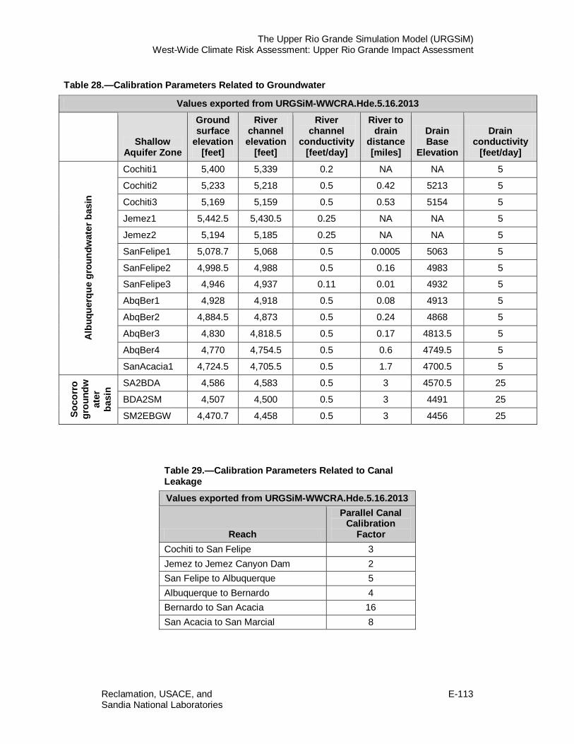
The Upper Rio Grande Simulation Model (URGSiM) West-Wide Climate Risk Assessment: Upper Rio Grande Impact Assessment
Reclamation, USACE, and E-113 Sandia National Laboratories
Table 28.—Calibration Parameters Related to Groundwater
Values exported from URGSiM-WWCRA.Hde.5.16.2013
Shallow
Aquifer Zone
Ground surface
elevation [feet]
River channel elevation
[feet]
River channel
conductivity [feet/day]
River to drain
distance [miles]
Drain Base
Elevation
Drain conductivity
[feet/day]
Alb
uque
rque
gro
undw
ater
bas
in
Cochiti1 5,400 5,339 0.2 NA NA 5
Cochiti2 5,233 5,218 0.5 0.42 5213 5
Cochiti3 5,169 5,159 0.5 0.53 5154 5
Jemez1 5,442.5 5,430.5 0.25 NA NA 5
Jemez2 5,194 5,185 0.25 NA NA 5
SanFelipe1 5,078.7 5,068 0.5 0.0005 5063 5
SanFelipe2 4,998.5 4,988 0.5 0.16 4983 5
SanFelipe3 4,946 4,937 0.11 0.01 4932 5
AbqBer1 4,928 4,918 0.5 0.08 4913 5
AbqBer2 4,884.5 4,873 0.5 0.24 4868 5
AbqBer3 4,830 4,818.5 0.5 0.17 4813.5 5
AbqBer4 4,770 4,754.5 0.5 0.6 4749.5 5
SanAcacia1 4,724.5 4,705.5 0.5 1.7 4700.5 5
Soco
rro
grou
ndw
ater
ba
sin
SA2BDA 4,586 4,583 0.5 3 4570.5 25
BDA2SM 4,507 4,500 0.5 3 4491 25
SM2EBGW 4,470.7 4,458 0.5 3 4456 25
Table 29.—Calibration Parameters Related to Canal Leakage
Values exported from URGSiM-WWCRA.Hde.5.16.2013
Reach
Parallel Canal Calibration
Factor Cochiti to San Felipe 3 Jemez to Jemez Canyon Dam 2 San Felipe to Albuquerque 5 Albuquerque to Bernardo 4 Bernardo to San Acacia 16 San Acacia to San Marcial 8

The Upper Rio Grande Simulation Model (URGSiM) West-Wide Climate Risk Assessment: Upper Rio Grande Impact Assessment
E-114 Reclamation, USACE, and
Sandia National Laboratories
Table 30.—Calibration Parameters Related to Reservoirs
Values exported from URGSiM-WWCRA.Hde.5.16.2013 Reservoir Parameter Value
Heron Heron native inflows factor 6.80%
El Vado La Puente reduction threshold [cfs] 2,000 La Puente reduction factor 35%
Abiquiu Abiquiu local inflows correlation to Jemez near Jemez Pueblo gage
54%
Cochiti Lake bottom (river bed in 1st shallow aquifer zone) conductivity [ft/da]
0.2
Jemez Jemez local inflow correlation to Jemez near Jemez Pueblo gage
52%
Jemez local inflow cutoff [cfs] 200 Elephant Butte
Shallow aquifer surface elevation San Marcial to Elephant Butte [ft]
4471
Caballo EB to Caballo ungaged effective area [acre] 26,000
Table 31.—Calibration Parameters Related to Reaches Values exported from URGSiM-WWCRA.Hde.5.16.2013
Reach Parameter Value El Vado to Abiquiu Ungaged correlation to Ojo Caliente @ La Madera 35% Abiquiu to Chamita Ungaged correlation to Ojo Caliente @ La Madera 3.5%
Riparian area [acres] 80 Lobatos to Cerro None Cerro to Taos Junction Bridge Ungaged correlation to Rio Pueblo de Taos near Rio
Grande 37% Taos Junction Bridge to Embudo Embudo Creek high flow threshold [cfs] 200
Embudo Creek high flow reduction 23% Embudo to Otowi Ungaged correlation to Rio Nambe below dam 120% Otowi to Cochiti Calibrated with Cochiti Reservoir Cochiti to San Felipe Ungaged correlation to Galisteo Creek 156%
Carriage water 15% San Felipe to Albuquerque Ungaged correlation to North Floodway Channel 92%
Carriage water 15% Albuquerque to Bernardo Carriage water 0% Bernardo to San Acacia Rio Puerco reduction factor 36%
Carriage water 15% San Acacia to San Marcial Carriage water 14% San Marcial to Elephant Butte Calibrated with Elephant Butte Reservoir
Elephant Butte to Caballo Calibrated with Caballo Reservoir

The Upper Rio Grande Simulation Model (URGSiM) West-Wide Climate Risk Assessment: Upper Rio Grande Impact Assessment
Reclamation, USACE, and E-115 Sandia National Laboratories
III.J. Additional Groundwater Data and Results
Figure 75 through Figure 77 and Table 32 through Table 42 provide additional groundwater data and results.
Figure 75.—Cumulative fluxes out of the groundwater system to the low flow conveyance channel for Rio Grande reaches from San Acacia to Elephant Butte as modeled by the coupled monthly timestep model, the URGWOM surface water model, and steady state values reported by Shafike (2005).
Figure 76.—Cumulative river leakage for Rio Grande reaches from San Acacia to Elephant Butte Reservoir as modeled by the coupled monthly timestep model, the URGWOM surface water model, and steady state values reported by Shafike (2005).
Cumulative LFCC GW gains between San Acacia and Elephant Butte reservoir 1975-1999
Jan 01, 1975 Jan 01, 1980 Jan 01, 1985 Jan 01, 1990 Jan 01, 1995 Jan 01, 2000
0
1,000,000
2,000,000
3,000,000
AF
URGWOM Shafike steady state Coupled SW GW
Cumulative river leakage between San Acacia and Elephant Butte reservoir 1975-1999
Jan 01, 1975 Jan 01, 1980 Jan 01, 1985 Jan 01, 1990 Jan 01, 1995 Jan 01, 2000
0
1,000,000
2,000,000
3,000,000
4,000,000
5,000,000
AF
URGWOM Shafike steady state Coupled SW GW

The Upper Rio Grande Simulation Model (URGSiM) West-Wide Climate Risk Assessment: Upper Rio Grande Impact Assessment
E-116 Reclamation, USACE, and
Sandia National Laboratories
Figure 77.—Cumulative riparian evaportranspiration for Rio Grande reaches from San Acacia to Elephant Butte Reservoir as modeled by the coupled monthly timestep model, the URGWOM surface water model, and steady state values reported by Shafike (2005).
Cumulative riparian ET between San Acacia and Elephant Butte reservoir 1975-1999
Jan 01, 1975 Jan 01, 1980 Jan 01, 1985 Jan 01, 1990 Jan 01, 1995 Jan 01, 20000
500,000
1,000,000
1,500,000
2,000,000AF
URGWOM Shafike steady state Coupled SW GW
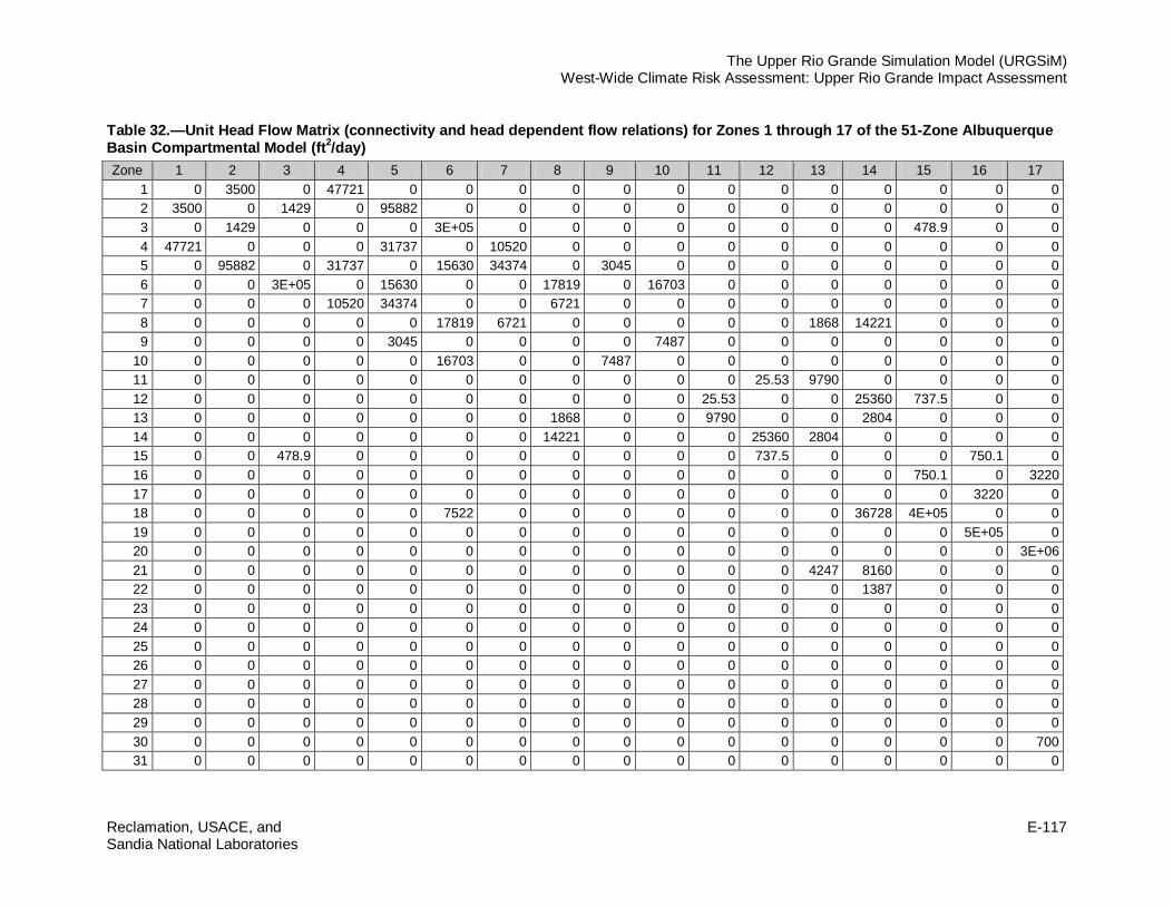
The Upper Rio Grande Simulation Model (URGSiM) West-Wide Climate Risk Assessment: Upper Rio Grande Impact Assessment
Reclamation, USACE, and E-117 Sandia National Laboratories
Table 32.—Unit Head Flow Matrix (connectivity and head dependent flow relations) for Zones 1 through 17 of the 51-Zone Albuquerque Basin Compartmental Model (ft2/day) Zone 1 2 3 4 5 6 7 8 9 10 11 12 13 14 15 16 17
1 0 3500 0 47721 0 0 0 0 0 0 0 0 0 0 0 0 0 2 3500 0 1429 0 95882 0 0 0 0 0 0 0 0 0 0 0 0 3 0 1429 0 0 0 3E+05 0 0 0 0 0 0 0 0 478.9 0 0 4 47721 0 0 0 31737 0 10520 0 0 0 0 0 0 0 0 0 0 5 0 95882 0 31737 0 15630 34374 0 3045 0 0 0 0 0 0 0 0 6 0 0 3E+05 0 15630 0 0 17819 0 16703 0 0 0 0 0 0 0 7 0 0 0 10520 34374 0 0 6721 0 0 0 0 0 0 0 0 0 8 0 0 0 0 0 17819 6721 0 0 0 0 0 1868 14221 0 0 0 9 0 0 0 0 3045 0 0 0 0 7487 0 0 0 0 0 0 0
10 0 0 0 0 0 16703 0 0 7487 0 0 0 0 0 0 0 0 11 0 0 0 0 0 0 0 0 0 0 0 25.53 9790 0 0 0 0 12 0 0 0 0 0 0 0 0 0 0 25.53 0 0 25360 737.5 0 0 13 0 0 0 0 0 0 0 1868 0 0 9790 0 0 2804 0 0 0 14 0 0 0 0 0 0 0 14221 0 0 0 25360 2804 0 0 0 0 15 0 0 478.9 0 0 0 0 0 0 0 0 737.5 0 0 0 750.1 0 16 0 0 0 0 0 0 0 0 0 0 0 0 0 0 750.1 0 3220 17 0 0 0 0 0 0 0 0 0 0 0 0 0 0 0 3220 0 18 0 0 0 0 0 7522 0 0 0 0 0 0 0 36728 4E+05 0 0 19 0 0 0 0 0 0 0 0 0 0 0 0 0 0 0 5E+05 0 20 0 0 0 0 0 0 0 0 0 0 0 0 0 0 0 0 3E+06 21 0 0 0 0 0 0 0 0 0 0 0 0 4247 8160 0 0 0 22 0 0 0 0 0 0 0 0 0 0 0 0 0 1387 0 0 0 23 0 0 0 0 0 0 0 0 0 0 0 0 0 0 0 0 0 24 0 0 0 0 0 0 0 0 0 0 0 0 0 0 0 0 0 25 0 0 0 0 0 0 0 0 0 0 0 0 0 0 0 0 0 26 0 0 0 0 0 0 0 0 0 0 0 0 0 0 0 0 0 27 0 0 0 0 0 0 0 0 0 0 0 0 0 0 0 0 0 28 0 0 0 0 0 0 0 0 0 0 0 0 0 0 0 0 0 29 0 0 0 0 0 0 0 0 0 0 0 0 0 0 0 0 0 30 0 0 0 0 0 0 0 0 0 0 0 0 0 0 0 0 700 31 0 0 0 0 0 0 0 0 0 0 0 0 0 0 0 0 0

The Upper Rio Grande Simulation Model (URGSiM) West-Wide Climate Risk Assessment: Upper Rio Grande Impact Assessment
E-118 Reclamation, USACE, and
Sandia National Laboratories
Table 32.—Unit Head Flow Matrix (connectivity and head dependent flow relations) for Zones 1 through 17 of the 51-Zone Albuquerque Basin Compartmental Model (ft2/day) Zone 1 2 3 4 5 6 7 8 9 10 11 12 13 14 15 16 17
32 0 0 0 0 0 0 0 0 0 0 0 0 0 0 0 0 0 33 0 0 0 0 0 0 0 0 0 0 0 0 0 0 0 0 0 34 0 0 0 0 0 0 0 0 0 0 0 0 0 0 0 0 0 35 0 0 0 0 0 0 0 0 0 0 0 0 0 0 0 0 0 36 0 0 0 0 0 0 0 0 0 0 0 0 0 0 0 0 0 37 0 0 0 0 0 0 0 0 0 0 0 0 0 0 0 0 0 38 0 0 0 0 0 0 0 0 0 0 0 0 0 0 0 0 0 39 0 0 0 0 0 0 0 0 0 0 0 0 0 0 0 0 0 40 0 0 0 0 0 0 0 0 0 0 0 0 0 0 0 0 0 41 0 0 0 0 0 0 0 0 0 0 0 0 0 0 0 0 0 42 0 0 0 0 0 0 0 0 0 0 0 0 0 0 0 0 0 43 0 0 0 0 0 0 0 0 0 0 0 0 0 0 0 0 0 44 0 0 0 0 0 0 0 0 0 0 0 0 0 0 0 0 0 45 0 0 0 0 0 0 0 0 0 0 0 0 0 0 0 0 0 46 0 0 0 0 0 0 0 0 0 0 0 0 0 0 0 0 0 47 0 0 0 0 0 0 0 0 0 0 0 0 0 0 0 0 0 48 0 0 0 0 0 0 0 0 0 0 0 0 0 0 0 0 0 49 0 0 0 0 0 0 0 0 0 0 0 0 0 0 0 0 0 50 0 0 0 0 0 0 0 0 0 0 0 0 0 0 0 0 0 51 0 0 0 0 0 0 0 0 0 0 0 0 0 0 0 0 0

The Upper Rio Grande Simulation Model (URGSiM) West-Wide Climate Risk Assessment: Upper Rio Grande Impact Assessment
Reclamation, USACE, and E-119 Sandia National Laboratories
Table 33.—Unit Head Flow Matrix (connectivity and head dependent flow relations) for Zones 18 through 34 of the 51-Zone Albuquerque Basin Compartmental Model (ft2/day) Zone 18 19 20 21 22 23 24 25 26 27 28 29 30 31 32 33 34
1 0 0 0 0 0 0 0 0 0 0 0 0 0 0 0 0 0 2 0 0 0 0 0 0 0 0 0 0 0 0 0 0 0 0 0 3 0 0 0 0 0 0 0 0 0 0 0 0 0 0 0 0 0 4 0 0 0 0 0 0 0 0 0 0 0 0 0 0 0 0 0 5 0 0 0 0 0 0 0 0 0 0 0 0 0 0 0 0 0 6 7522 0 0 0 0 0 0 0 0 0 0 0 0 0 0 0 0 7 0 0 0 0 0 0 0 0 0 0 0 0 0 0 0 0 0 8 0 0 0 0 0 0 0 0 0 0 0 0 0 0 0 0 0 9 0 0 0 0 0 0 0 0 0 0 0 0 0 0 0 0 0
10 0 0 0 0 0 0 0 0 0 0 0 0 0 0 0 0 0 11 0 0 0 0 0 0 0 0 0 0 0 0 0 0 0 0 0 12 0 0 0 0 0 0 0 0 0 0 0 0 0 0 0 0 0 13 0 0 0 4247 0 0 0 0 0 0 0 0 0 0 0 0 0 14 36728 0 0 8160 1387 0 0 0 0 0 0 0 0 0 0 0 0 15 4E+05 0 0 0 0 0 0 0 0 0 0 0 0 0 0 0 0 16 0 5E+05 0 0 0 0 0 0 0 0 0 0 0 0 0 0 0 17 0 0 3E+06 0 0 0 0 0 0 0 0 0 700 0 0 0 0 18 0 13173 0 0 0 0 0 0 1934 5416 0 0 0 0 0 0 0 19 13173 0 57557 0 5298 0 0 0 0 12161 0 0 0 0 0 0 0 20 0 57557 0 0 0 0 2092 0 0 0 38966 0 0 0 0 0 21074 21 0 0 0 0 3991 812.5 0 0 0 0 0 0 0 0 0 0 0 22 0 5298 0 3991 0 3986 7479 0 0 0 0 0 0 0 0 0 0 23 0 0 0 812.5 3986 0 0 1050 0 0 0 0 0 0 0 0 0 24 0 0 2092 0 7479 0 0 5517 0 0 0 0 0 0 0 0 0 25 0 0 0 0 0 1050 5517 0 0 0 0 0 0 0 0 0 0 26 1934 0 0 0 0 0 0 0 0 0 0 0 0 0 0 0 0 27 5416 12161 0 0 0 0 0 0 0 0 14399 4016 0 0 0 0 0 28 0 0 38966 0 0 0 0 0 0 14399 0 2960 0 0 0 0 0 29 0 0 0 0 0 0 0 0 0 4016 2960 0 0 0 0 0 0 30 0 0 0 0 0 0 0 0 0 0 0 0 0 1836 0 0 2E+05 31 0 0 0 0 0 0 0 0 0 0 0 0 1836 0 1612 0 0

The Upper Rio Grande Simulation Model (URGSiM) West-Wide Climate Risk Assessment: Upper Rio Grande Impact Assessment
E-120 Reclamation, USACE, and
Sandia National Laboratories
Table 33.—Unit Head Flow Matrix (connectivity and head dependent flow relations) for Zones 18 through 34 of the 51-Zone Albuquerque Basin Compartmental Model (ft2/day) Zone 18 19 20 21 22 23 24 25 26 27 28 29 30 31 32 33 34
32 0 0 0 0 0 0 0 0 0 0 0 0 0 1612 0 952.5 0 33 0 0 0 0 0 0 0 0 0 0 0 0 0 0 952.5 0 0 34 0 0 21074 0 0 0 0 0 0 0 0 0 2E+05 0 0 0 0 35 0 0 0 0 0 0 0 0 0 0 0 0 0 2E+06 0 0 6141 36 0 0 0 0 0 0 0 0 0 0 0 0 0 0 3E+05 0 0 37 0 0 0 0 0 0 0 0 0 0 0 0 0 0 0 3E+05 0 38 0 0 0 0 0 0 10646 0 0 0 0 0 0 0 0 0 78761 39 0 0 0 0 0 0 0 1049 0 0 0 0 0 0 0 0 0 40 0 0 0 0 0 0 0 0 0 0 0 0 0 0 0 0 0 41 0 0 0 0 0 0 0 0 0 0 0 0 0 0 0 0 0 42 0 0 0 0 0 0 0 0 0 0 0 0 0 0 0 0 0 43 0 0 0 0 0 0 0 0 0 0 0 0 0 0 0 0 0 44 0 0 0 0 0 0 0 0 0 0 1559 2155 0 0 0 0 16495 45 0 0 0 0 0 0 0 0 0 0 0 0 0 0 0 0 0 46 0 0 0 0 0 0 0 0 0 0 0 0 0 0 0 0 0 47 0 0 0 0 0 0 0 0 0 0 0 0 0 0 0 0 0 48 0 0 0 0 0 0 0 0 0 0 0 0 0 0 0 950.8 0 49 0 0 0 0 0 0 0 0 0 0 0 0 0 0 0 0 0 50 0 0 0 0 0 0 0 0 0 0 0 0 0 0 0 0 0 51 0 0 0 0 0 0 0 0 0 0 0 0 0 0 0 0 0

The Upper Rio Grande Simulation Model (URGSiM) West-Wide Climate Risk Assessment: Upper Rio Grande Impact Assessment
Reclamation, USACE, and E-121 Sandia National Laboratories
Table 34.—Unit Head Flow Matrix (connectivity and head dependent flow relations) for Zones 35 through 51 of the 51-Zone Albuquerque Basin Compartmental Model (ft2/day) Zone 35 36 37 38 39 40 41 42 43 44 45 46 47 48 49 50 51
1 0 0 0 0 0 0 0 0 0 0 0 0 0 0 0 0 0 2 0 0 0 0 0 0 0 0 0 0 0 0 0 0 0 0 0 3 0 0 0 0 0 0 0 0 0 0 0 0 0 0 0 0 0 4 0 0 0 0 0 0 0 0 0 0 0 0 0 0 0 0 0 5 0 0 0 0 0 0 0 0 0 0 0 0 0 0 0 0 0 6 0 0 0 0 0 0 0 0 0 0 0 0 0 0 0 0 0
7 0 0 0 0 0 0 0 0 0 0 0 0 0 0 0 0 0 8 0 0 0 0 0 0 0 0 0 0 0 0 0 0 0 0 0 9 0 0 0 0 0 0 0 0 0 0 0 0 0 0 0 0 0
10 0 0 0 0 0 0 0 0 0 0 0 0 0 0 0 0 0 11 0 0 0 0 0 0 0 0 0 0 0 0 0 0 0 0 0 12 0 0 0 0 0 0 0 0 0 0 0 0 0 0 0 0 0 13 0 0 0 0 0 0 0 0 0 0 0 0 0 0 0 0 0 14 0 0 0 0 0 0 0 0 0 0 0 0 0 0 0 0 0
15 0 0 0 0 0 0 0 0 0 0 0 0 0 0 0 0 0 16 0 0 0 0 0 0 0 0 0 0 0 0 0 0 0 0 0 17 0 0 0 0 0 0 0 0 0 0 0 0 0 0 0 0 0 18 0 0 0 0 0 0 0 0 0 0 0 0 0 0 0 0 0 19 0 0 0 0 0 0 0 0 0 0 0 0 0 0 0 0 0 20 0 0 0 0 0 0 0 0 0 0 0 0 0 0 0 0 0 21 0 0 0 0 0 0 0 0 0 0 0 0 0 0 0 0 0 22 0 0 0 0 0 0 0 0 0 0 0 0 0 0 0 0 0
23 0 0 0 0 0 0 0 0 0 0 0 0 0 0 0 0 0 24 0 0 0 10646 0 0 0 0 0 0 0 0 0 0 0 0 0 25 0 0 0 0 1049 0 0 0 0 0 0 0 0 0 0 0 0 26 0 0 0 0 0 0 0 0 0 0 0 0 0 0 0 0 0

The Upper Rio Grande Simulation Model (URGSiM) West-Wide Climate Risk Assessment: Upper Rio Grande Impact Assessment
E-122 Reclamation, USACE, and
Sandia National Laboratories
Table 34.—Unit Head Flow Matrix (connectivity and head dependent flow relations) for Zones 35 through 51 of the 51-Zone Albuquerque Basin Compartmental Model (ft2/day) Zone 35 36 37 38 39 40 41 42 43 44 45 46 47 48 49 50 51
27 0 0 0 0 0 0 0 0 0 0 0 0 0 0 0 0 0 28 0 0 0 0 0 0 0 0 0 1559 0 0 0 0 0 0 0 29 0 0 0 0 0 0 0 0 0 2155 0 0 0 0 0 0 0 30 0 0 0 0 0 0 0 0 0 0 0 0 0 0 0 0 0 31 2E+06 0 0 0 0 0 0 0 0 0 0 0 0 0 0 0 0 32 0 3E+05 0 0 0 0 0 0 0 0 0 0 0 0 0 0 0
33 0 0 3E+05 0 0 0 0 0 0 0 0 0 0 950.8 0 0 0 34 6141 0 0 78761 0 0 0 0 0 16495 0 0 0 0 0 0 0 35 0 16024 0 0 0 2E+05 0 0 0 0 8794 0 0 0 0 0 0 36 16024 0 10111 0 0 0 0 50668 0 0 0 20383 0 0 0 0 0 37 0 10111 0 0 0 0 0 0 13360 0 0 0 11638 0 5442 0 0 38 0 0 0 0 4651 4406 0 0 0 0 0 0 0 0 0 0 0 39 0 0 0 4651 0 2164 512.8 0 0 0 0 0 0 0 0 0 0 40 2E+05 0 0 4406 2164 0 10433 6775 0 0 0 0 0 0 0 0 0
41 0 0 0 0 512.8 10433 0 465.4 879.1 0 0 0 0 0 0 201.7 0 42 0 50668 0 0 0 6775 465.4 0 4857 0 0 0 0 0 0 0 0 43 0 0 13360 0 0 0 879.1 4857 0 0 0 0 0 0 0 38597 0 44 0 0 0 0 0 0 0 0 0 0 12079 0 0 0 0 0 0 45 8794 0 0 0 0 0 0 0 0 12079 0 6504 0 0 0 0 0 46 0 20383 0 0 0 0 0 0 0 0 6504 0 4957 0 0 0 0 47 0 0 11638 0 0 0 0 0 0 0 0 4957 0 0 0 0 1341 48 0 0 0 0 0 0 0 0 0 0 0 0 0 0 1E+05 0 0
49 0 0 5442 0 0 0 0 0 0 0 0 0 0 1E+05 0 4934 6536 50 0 0 0 0 0 0 201.7 0 38597 0 0 0 0 0 4934 0 0 51 0 0 0 0 0 0 0 0 0 0 0 0 1341 0 6536 0 0

The Upper Rio Grande Simulation Model (URGSiM) West-Wide Climate Risk Assessment: Upper Rio Grande Impact Assessment
Reclamation, USACE, and E-123 Sandia National Laboratories
Table 35.—Zone Bottom Elevations (ft above mean sea level), Areal Extent (km2), and Initial Heads (feet above mean sea level) for the Spatially Aggregated Albuquerque Basin Groundwater Model Zone Bottom Elevation (ft msl) Area (km2) Jan 1975 Heads (ft)
1 5159.2 16 5239.7 2 5129.3 29 5209.5 3 5079.1 64 5158.4 4 2860.7 80 5252.6 5 2277.4 87 5219.1 6 -728.1 137 5162.5 7 1465 107 5227.4 8 -2661 183 5174.9 9 3899.2 79 5292.9 10 2617.8 94 5206.4 11 5316 83 5430.4 12 5083.4 41 5172.1 13 3182.4 305 5368.9 14 -68.441 231 5134.6 15 4987.3 100 5066.3 16 4918.4 56 4992 17 4887.2 74 4945.3 18 -751.43 182 5070.5 19 -6335.4 88 4988.1 20 -5916 106 4942.7 21 2519.3 122 5163.5 22 -966.25 206 5024.1 23 1635.3 153 5037.6 24 -2834.3 68 4955.1 25 1066.9 104 4965.2 26 2522.2 54 5226.9 27 780.59 36 4990.9 28 -2424 85 4928.8 29 3135.5 92 5020.5 30 4845.7 73 4920.3 31 4792.4 120 4874.2 32 4734.2 172 4819.2 33 4673.5 109 4756 34 -3002.2 108 4916 35 -4230.1 202 4874.1 36 -3833.2 265 4820.4 37 -1637.1 194 4759.5 38 -1127.3 67 4919.6 39 2358.3 116 4916 40 -2968.1 272 4873.5 41 -1289.6 756 4875

The Upper Rio Grande Simulation Model (URGSiM) West-Wide Climate Risk Assessment: Upper Rio Grande Impact Assessment
E-124 Reclamation, USACE, and
Sandia National Laboratories
Table 35.—Zone Bottom Elevations (ft above mean sea level), Areal Extent (km2), and Initial Heads (feet above mean sea level) for the Spatially Aggregated Albuquerque Basin Groundwater Model Zone Bottom Elevation (ft msl) Area (km2) Jan 1975 Heads (ft)
42 -4500.1 272 4822.2 43 -3190.2 213 4776 44 -2977.6 100 4922.5 45 -415.52 139 4894.1 46 -458.59 258 4836.3 47 1364.6 205 4791 48 4627.7 69 4707.2 49 1888.4 140 4713.2 50 1817.5 104 4774.2 51 3417.6 65 4727.5
Table 36.—Zone Bottom Elevations (ft msl), Areal Extent (square kilometers), and Initial Heads (feet above mean sea level) for the Spatially Aggregated Espanola Basin Groundwater Model
Zone Bottom Elevation (feet amsl) Area (mile2) 1975 Head (feet amsl)
1 355 74 5955
2 96 76 5696
3 401 44 6001
4 320 23 5920
5 96 52 5696
6 256 41 5856
7 611 77 6211
8 -111 90 5489
9 406 28 6006
10 963 70 6563
11 143 25 5743
12 551 77 6151
13 930 35 6530
14 5400 22 5600
15 5185 16 5385
16 5480 5 5680
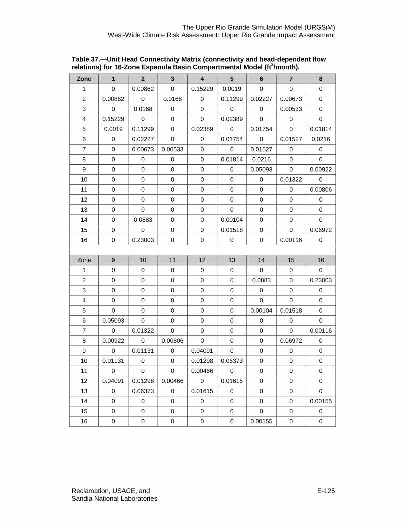
The Upper Rio Grande Simulation Model (URGSiM) West-Wide Climate Risk Assessment: Upper Rio Grande Impact Assessment
Reclamation, USACE, and E-125 Sandia National Laboratories
Table 37.—Unit Head Connectivity Matrix (connectivity and head-dependent flow relations) for 16-Zone Espanola Basin Compartmental Model (ft2/month).
Zone 1 2 3 4 5 6 7 8 1 0 0.00862 0 0.15229 0.0019 0 0 0 2 0.00862 0 0.0168 0 0.11299 0.02227 0.00673 0 3 0 0.0168 0 0 0 0 0.00533 0 4 0.15229 0 0 0 0.02389 0 0 0 5 0.0019 0.11299 0 0.02389 0 0.01754 0 0.01814 6 0 0.02227 0 0 0.01754 0 0.01527 0.0216
7 0 0.00673 0.00533 0 0 0.01527 0 0 8 0 0 0 0 0.01814 0.0216 0 0 9 0 0 0 0 0 0.05093 0 0.00922
10 0 0 0 0 0 0 0.01322 0 11 0 0 0 0 0 0 0 0.00806 12 0 0 0 0 0 0 0 0 13 0 0 0 0 0 0 0 0 14 0 0.0883 0 0 0.00104 0 0 0
15 0 0 0 0 0.01518 0 0 0.06972 16 0 0.23003 0 0 0 0 0.00116 0
Zone 9 10 11 12 13 14 15 16
1 0 0 0 0 0 0 0 0 2 0 0 0 0 0 0.0883 0 0.23003 3 0 0 0 0 0 0 0 0 4 0 0 0 0 0 0 0 0
5 0 0 0 0 0 0.00104 0.01518 0 6 0.05093 0 0 0 0 0 0 0 7 0 0.01322 0 0 0 0 0 0.00116 8 0.00922 0 0.00806 0 0 0 0.06972 0 9 0 0.01131 0 0.04091 0 0 0 0
10 0.01131 0 0 0.01298 0.06373 0 0 0 11 0 0 0 0.00466 0 0 0 0 12 0.04091 0.01298 0.00466 0 0.01615 0 0 0
13 0 0.06373 0 0.01615 0 0 0 0 14 0 0 0 0 0 0 0 0.00155 15 0 0 0 0 0 0 0 0 16 0 0 0 0 0 0.00155 0 0
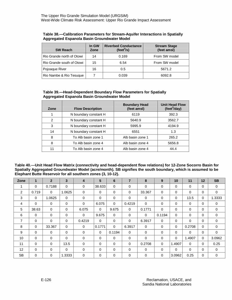
The Upper Rio Grande Simulation Model (URGSiM) West-Wide Climate Risk Assessment: Upper Rio Grande Impact Assessment
E-126 Reclamation, USACE, and
Sandia National Laboratories
Table 38.—Calibration Parameters for Stream-Aquifer Interactions in Spatially Aggregated Espanola Basin Groundwater Model
SW Reach In GW Zone
Riverbed Conductance (feet2/s)
Stream Stage (feet amsl)
Rio Grande north of Otowi 14 0.169 From SW model
Rio Grande south of Otowi 15 6.54 From SW model
Pojoaque River 16 0.5 5671.2
Rio Nambe & Rio Tesuque 7 0.039 6092.8
Table 39.—Head-Dependent Boundary Flow Parameters for Spatially Aggregated Espanola Basin Groundwater Model
Zone Flow Description Boundary Head
(feet amsl) Unit Head Flow
(feet2/day) 1 N boundary constant H 6119 392.3 2 N boundary constant H 5640.9 3562.7 3 N boundary constant H 5995.9 4194.9 14 N boundary constant H 6551 1.3 8 To Alb basin zone 1 Alb basin zone 1 265.2 8 To Alb basin zone 4 Alb basin zone 4 5656.8 11 To Alb basin zone 4 Alb basin zone 4 44.4
Table 40.—Unit Head Flow Matrix (connectivity and head-dependent flow relations) for 12-Zone Socorro Basin for Spatially Aggregated Groundwater Model (acre/month). SB signifies the south boundary, which is assumed to be Elephant Butte Reservoir for all southern zones (3, 10-12).
Zone 1 2 3 4 5 6 7 8 9 10 11 12 SB 1 0 0.7188 0 0 38.633 0 0 0 0 0 0 0 0 2 0.719 0 1.0625 0 0 0 0 33.367 0 0 0 0 0 3 0 1.0625 0 0 0 0 0 0 0 0 13.5 0 1.3333 4 0 0 0 0 6.075 0 0.4219 0 0 0 0 0 0 5 38.63 0 0 6.075 0 9.675 0 0.1771 0 0 0 0 0 6 0 0 0 0 9.675 0 0 0 0.1194 0 0 0 0 7 0 0 0 0.4219 0 0 0 6.3917 0 0 0 0 0
8 0 33.367 0 0 0.1771 0 6.3917 0 0 0 0.2708 0 0 9 0 0 0 0 0 0.1194 0 0 0 0 0 0 0
10 0 0 0 0 0 0 0 0 0 0 1.4907 0 3.0962 11 0 0 13.5 0 0 0 0 0.2708 0 1.4907 0 0 0.25 12 0 0 0 0 0 0 0 0 0 0 0 0 0 SB 0 0 1.3333 0 0 0 0 0 0 3.0962 0.25 0 0
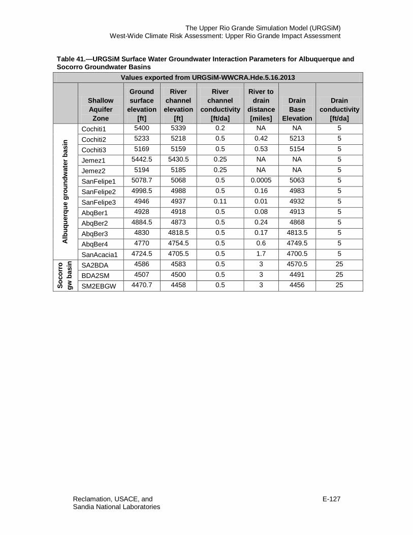
The Upper Rio Grande Simulation Model (URGSiM) West-Wide Climate Risk Assessment: Upper Rio Grande Impact Assessment
Reclamation, USACE, and E-127 Sandia National Laboratories
Table 41.—URGSiM Surface Water Groundwater Interaction Parameters for Albuquerque and Socorro Groundwater Basins
Values exported from URGSiM-WWCRA.Hde.5.16.2013
Shallow Aquifer Zone
Ground surface
elevation [ft]
River channel elevation
[ft]
River channel
conductivity [ft/da]
River to drain
distance [miles]
Drain Base
Elevation
Drain conductivity
[ft/da]
Alb
uque
rque
gro
undw
ater
bas
in
Cochiti1 5400 5339 0.2 NA NA 5
Cochiti2 5233 5218 0.5 0.42 5213 5
Cochiti3 5169 5159 0.5 0.53 5154 5
Jemez1 5442.5 5430.5 0.25 NA NA 5
Jemez2 5194 5185 0.25 NA NA 5
SanFelipe1 5078.7 5068 0.5 0.0005 5063 5
SanFelipe2 4998.5 4988 0.5 0.16 4983 5
SanFelipe3 4946 4937 0.11 0.01 4932 5
AbqBer1 4928 4918 0.5 0.08 4913 5
AbqBer2 4884.5 4873 0.5 0.24 4868 5
AbqBer3 4830 4818.5 0.5 0.17 4813.5 5
AbqBer4 4770 4754.5 0.5 0.6 4749.5 5
SanAcacia1 4724.5 4705.5 0.5 1.7 4700.5 5
Soco
rro
gw b
asin
SA2BDA 4586 4583 0.5 3 4570.5 25
BDA2SM 4507 4500 0.5 3 4491 25
SM2EBGW 4470.7 4458 0.5 3 4456 25

The Upper Rio Grande Simulation Model (URGSiM) West-Wide Climate Risk Assessment: Upper Rio Grande Impact Assessment
E-128 Reclamation, USACE, and
Sandia National Laboratories
Table 42.—Estimated Groundwater Head Values for January 1975
Groundwater Parameter Groundwater Zone
Number Unit Value Esp Basin Initial GW Heads 1 ft 5955.2 Esp Basin Initial GW Heads 2 ft 5696.2 Esp Basin Initial GW Heads 3 ft 6001 Esp Basin Initial GW Heads 4 ft 5919.9 Esp Basin Initial GW Heads 5 ft 5695.6 Esp Basin Initial GW Heads 6 ft 5855.9 Esp Basin Initial GW Heads 7 ft 6210.8 Esp Basin Initial GW Heads 8 ft 5489.1 Esp Basin Initial GW Heads 9 ft 6005.7 Esp Basin Initial GW Heads 10 ft 6562.5 Esp Basin Initial GW Heads 11 ft 5743 Esp Basin Initial GW Heads 12 ft 6150.7 Esp Basin Initial GW Heads 13 ft 6529.6 Esp Basin Initial GW Heads 14 ft 5599.7 Esp Basin Initial GW Heads 15 ft 5384.9 Esp Basin Initial GW Heads 16 ft 5679.7 Alb Basin Initial GW Heads 1 ft 5239.7 Alb Basin Initial GW Heads 2 ft 5209.5 Alb Basin Initial GW Heads 3 ft 5158.4 Alb Basin Initial GW Heads 4 ft 5252.6 Alb Basin Initial GW Heads 5 ft 5219.1 Alb Basin Initial GW Heads 6 ft 5162.5 Alb Basin Initial GW Heads 7 ft 5227.4 Alb Basin Initial GW Heads 8 ft 5174.9 Alb Basin Initial GW Heads 9 ft 5292.9 Alb Basin Initial GW Heads 10 ft 5206.4 Alb Basin Initial GW Heads 11 ft 5430.4 Alb Basin Initial GW Heads 12 ft 5172.1 Alb Basin Initial GW Heads 13 ft 5368.9 Alb Basin Initial GW Heads 14 ft 5134.6 Alb Basin Initial GW Heads 15 ft 5066.3 Alb Basin Initial GW Heads 16 ft 4992 Alb Basin Initial GW Heads 17 ft 4933 Alb Basin Initial GW Heads 18 ft 5070.5 Alb Basin Initial GW Heads 19 ft 4988.1 Alb Basin Initial GW Heads 20 ft 4934 Alb Basin Initial GW Heads 21 ft 5163.5 Alb Basin Initial GW Heads 22 ft 5024.1 Alb Basin Initial GW Heads 23 ft 5037.6 Alb Basin Initial GW Heads 24 ft 4955.1 Alb Basin Initial GW Heads 25 ft 4965.2 Alb Basin Initial GW Heads 26 ft 5226.9

The Upper Rio Grande Simulation Model (URGSiM) West-Wide Climate Risk Assessment: Upper Rio Grande Impact Assessment
Reclamation, USACE, and E-129 Sandia National Laboratories
Table 42.—Estimated Groundwater Head Values for January 1975
Groundwater Parameter Groundwater Zone
Number Unit Value Alb Basin Initial GW Heads 27 ft 4990.9 Alb Basin Initial GW Heads 28 ft 4928.8 Alb Basin Initial GW Heads 29 ft 5020.5 Alb Basin Initial GW Heads 30 ft 4920.3 Alb Basin Initial GW Heads 31 ft 4874.2 Alb Basin Initial GW Heads 32 ft 4819.2 Alb Basin Initial GW Heads 33 ft 4756 Alb Basin Initial GW Heads 34 ft 4916 Alb Basin Initial GW Heads 35 ft 4874.1 Alb Basin Initial GW Heads 36 ft 4820.4 Alb Basin Initial GW Heads 37 ft 4759.5 Alb Basin Initial GW Heads 38 ft 4919.6 Alb Basin Initial GW Heads 39 ft 4916 Alb Basin Initial GW Heads 40 ft 4873.5 Alb Basin Initial GW Heads 41 ft 4875 Alb Basin Initial GW Heads 42 ft 4822.2 Alb Basin Initial GW Heads 43 ft 4776 Alb Basin Initial GW Heads 44 ft 4922.5 Alb Basin Initial GW Heads 45 ft 4894.1 Alb Basin Initial GW Heads 46 ft 4836.3 Alb Basin Initial GW Heads 47 ft 4791 Alb Basin Initial GW Heads 48 ft 4707.2 Alb Basin Initial GW Heads 49 ft 4713.2 Alb Basin Initial GW Heads 50 ft 4774.2 Alb Basin Initial GW Heads 51 ft 4727.5 Soc Basin Initial GW Heads 1 ft 4575 Soc Basin Initial GW Heads 2 ft 4496 Soc Basin Initial GW Heads 3 ft 4459 Soc Basin Initial GW Heads 4 ft 4635 Soc Basin Initial GW Heads 5 ft 4585 Soc Basin Initial GW Heads 6 ft 4595 Soc Basin Initial GW Heads 7 ft 4556 Soc Basin Initial GW Heads 8 ft 4506 Soc Basin Initial GW Heads 9 ft 4515 Soc Basin Initial GW Heads 10 ft 4878 Soc Basin Initial GW Heads 11 ft 4469 Soc Basin Initial GW Heads 12 ft 4469

The Upper Rio Grande Simulation Model (URGSiM) West-Wide Climate Risk Assessment: Upper Rio Grande Impact Assessment
E-130 Reclamation, USACE, and
Sandia National Laboratories
IV. Bibliography Allen, R. G., L. S. Pereira, D. Raes, and Smith, M., 1998. Crop
evapotranspiration —Guidelines for computing crop water requirements. FAO Irrigation and Drainage Paper 56. Rome: FAO - Food and Agriculture Organization of the United Nations.
Baird, K. J. and T. I.Maddock, 2005. Simulating Riparian Evapotranspiration: a New Methodology and Application for Groundwater Models. Journal of Hydrology, Volume 312, Issues 1–4, Pages 176–190. October 10, 2005, Online: <http://www.sciencedirect.com/science/article/pii/S0022169405000879>
Barroll, P. and P. Burck, 2006. Documentation of the OSE Taos Area Calibrated Groundwater Flow Model T17.0. New Mexico Office of the State Engineer Hydrology Bureau Report 06-04. January 11, 2006. http://www.ose.state.nm.us/publications/hydrology/TaosHBR-06-04.pdf
Boroughs, C., 2009. Estimation of Initial Conditions for URGWOM Planning Model Simulations Starting on January 1, 2010. Albuquerque: Technical Memorandum to Leann Towne, Reclamation—PHVA Work Group and April Sanders, United States Army Corps of Engineers.
______, 2010. Notes—July 26-28 2010 URGWOM Technical Team Field Trip to the San Luis Valley. Albuquerque: Technical Memo to URGWOM Technical Team.
Brower, A., 2008. ET Toolbox: Evapotranspiration Toolbox for the Middle Rio Grande, a Water Resources Decision Support Tool. Denver: Water and Environmental Resources Division, Technical Service Center, Reclamation.
Cleverly, J. R., C. N. Dahm, J. R. Thibault, D. E. McDonnell, and J. E. Coonrod, 2006. Riparian Ecohydrology: Regulation of Water Flux from the Ground to the Atmosphere in the Middle Rio Grande, New Mexico. Volume 20, Issue 15, Pages 3207–3225, 15 October 2006 Hydrological Processes.
Frenzel, P. F., 1995. Geohydrology and Simulation of Groundwater Flow near Los Alamos, North-Central New Mexico. Albuquerque: U.S. Geological Survey Water-Resources Investigations Report 95-4091.
Hargreaves, G. H. and R. G.Allen, 2003. History and Evaluation of Hargreaves Evapotranspiration Equation. Journal of Irrigation and Drainage Engineering, January – February 2003, Pages 53-63.

The Upper Rio Grande Simulation Model (URGSiM) West-Wide Climate Risk Assessment: Upper Rio Grande Impact Assessment
Reclamation, USACE, and E-131 Sandia National Laboratories
Hargreaves, G. H. and Z. A.Samani, 1985. Reference Crop Evapotranspiration from Temperature. Applied Engineering in Agriculture, Volume 1, Number. 2, Pages 96-99.
Hearne, G. and J. Dewey, 1988. Hydrologic Analysis of the Rio Grande Basin North of Embudo, New Mexico, Colorado and New Mexico. Denver: United States Geological Survey.
Jemez y Sangre Water Planning Council, 2003, Jemez y Sangre Regional Water Plan. Prepared by Daniel B. Stephens and Associates, Albuquerque, New Mexico, in association with Amy C. Lewis, Santa Fe, New Mexico. Available October 2006 at http://www.ose.state.nm.us/water-info/NMWaterPlanning/regions/jemezysangre/jys_sec1-5.pdf
Jensen, M., 1998. Coefficients for Vegetative Evapotranspiration and Open Water Evaporation for the Lower Colorado River Accountintg System. Boulder City, Nevada: Bureau of Reclamation.
McAda, D. P., and P. Barroll, 2002. Simulation of Groundwater Flow in the Middle Rio Grande Between Cochiti and San Acacia, New Mexico. Albuquerque: U.S. Geological Survey.
McAda, D. and M. Wasiolek, 1988. Simulation of the Regional Geohydrology of the Tesuque Aquifer System near Santa Fe, New Mexico. United States Geological Survey, Albuquerque, New Mexico.
McDonald, M. and Harbaugh, A., 1988. A Modular Thre Dimensional Finit Difference Groundwater Flow Model. In U.S. Survey, U.S. Geological Survey Techniques of Water Resources Investigations, Book 6 (Chapter A1).
Miller, L., and J. Stiles, 2006, Water Resources Data, New Mexico, Water Year 2005. Water-Data Report NM-05-1. United States Geological Survey, New Mexico Water Science Center, Albuquerque, New Mexico. http://pubs.usgs.gov/wdr/2005/wdr-nm-05-1/
New Mexico State University, nd. Weather data. <: http://hydrology1. nmsu.edu/cgi-shl/cns/uberpage.pl?selected=2>. Accessed 1/10/2012.
Penman, H.L. 1948. Natural evaporation from open water, bare soil and grass. Proc. Roy. Soc. London A(194), S. 120-145.
Reclamation, 1997. Middle Rio Grande Water Assessment. Estimates of Consumptive Use Requirements for Irrigated Agriculture and Riparian Vegetation. Volume II Appendices 1-7. Albuquerque, New Mexico.

The Upper Rio Grande Simulation Model (URGSiM) West-Wide Climate Risk Assessment: Upper Rio Grande Impact Assessment
E-132 Reclamation, USACE, and
Sandia National Laboratories
______, 1999. Revised San Juan- Chama Firm Yield (DRAFT). Upper Colorado Region. Albuquerque, New Mexico.
______, 2002. Effects of LFCC Experimental Operations: Water Diversions from the Rio Grande and Parrot Feather Removal. Biological Assesment, Albuquerque, New Mexico
______, 2006. San Juan-Chama Water Contract Amendments with City of Santa Fe, County of Santa Fe, County of Los Alamos, Town of Taos, Village of Taos Ski Valley, Village of Losa Lunas, and City of Espanola. Environmental Assessment, Albuquerque, New Mexico.
Reclamation, 2012. Daily data from ET Toolbox website. <http://www.usbr.gov/pmts/rivers/awards/Nm2/rg/PROD/wx/txt/archive/> downloaded 2/27/2012.
______, 2013. Upper Rio Grande System and Operations. Upper Colorado Region. Albuquerque, New Mexico.
Roach, J. D., 2007. Integrated Surface Water Groundwater Modeling in the Upper Rio Grande in Support of Scenario Analysis. University of Arizona. Tucson, Arizona.
______, 2009. Stochastic Hydrologic Analysis of the Upper Rio Grande Surface Water System in New Mexico. Report to Reclamation. Sandia National Laboratories. Albuquerque , New Mexico.
______, 2011. Expected Hydrologic Impacts Associated with Increased Conservation Storage at El Vado Reservoir, New Mexico. Albuquerque, New Mexico.
______ 2012. Evapotranspiration Calculations in the Upper Rio Grande Simulation Model (URGSiM). Sandia National Laboratories. Albuquerque, New Mexico
Roach, J. D., and V. C Tidwell, 2009. A Compartmental-Spatial System Dynamics Approach to Ground Water Modeling. Ground Water. Volume 47, Number 5, Pages 686-698. September-October 2009. Online <doi: 10.1111/j.1745-6584.2009.00580.x>.
Sammis, T. W., C. L. Mapel, D. G. Lugg, R. R. Lansford, and J. T. McGuckin. 1985. Evapotranspiration Crop Coefficients Predicted Using Growing-Degre Days. Transactions of the ASAE. American Society of Agricultural Engineers, Volume 28, Number 3, Pages 773-780.

The Upper Rio Grande Simulation Model (URGSiM) West-Wide Climate Risk Assessment: Upper Rio Grande Impact Assessment
Reclamation, USACE, and E-133 Sandia National Laboratories
Shafike, N. G. 2005 (groundwater). Steady State Groundwater Heads Simulated for the Socorro Groundwater Basin. Personal email communication.
Shafike, N. G. 2005. Linked Surface Water and Groundwater Model for Socorro and San Marcial Basins between San Acacia and Elephant Butte Reservoir. Albuquerque: Appendix J in Upper Rio Grande Water Operations Review DEIS, pp. J-59 to J-94. <http://w3.spa.usace.army.mil/urgwops/feis/Volume%202/URGWOPS%20FEIS%20Appendix%20J.pdf>.
Sidlow, M. 2006. Personal Communication, from Marc Sidlow, Hydraulic Engineer, U.S. Army Corps of Engineers, to Jesse Roach, Sandia National Laboratories, via email. November 14.
Task Committee on Standardization of Reference Evapotranspiration, 2005. The ASCE Standardized Reference Evapotranspiration Equation. ASC EWRI.
Tetra Tech Inc, 2003. Rio Grande Seepage Study Report, Taos Box Canyon. Final Report for Reclamation. Tetra Tech ISG Project No. P06000-0023-01.
U.S. Army Corps of Engineers, U.S. Geological Survey, Bureau of Reclamation, U.S. Fish and Wildlife Service, U.S. Bureau of Indian Affairs, and International Boundary and Water Commission, 2002. Upper Rio Grande Water Operations Model Model Documentation, Draft. Model Documentation, Albuquerque.
United States Census Bureau, 2007, City, County, and State Population Estimates for New Mexico, 1990, 2000, and 2005. URL accessed February 14, 2007: <http://www.census.gov>.
United States Department of Agriculture, 1970. Irrigation Water Requirements. Technical Release No. 21. Washington DC: U.S. Department of Agriculture Soil Conservation Service.
Western Regional Climate Center, 2013. Bosque Del Apache, New Mexico. Climate data. http://www.wrcc.dri.edu/cgi-bin/cliMAIN.pl?nm1138. Accessed 1/10/2012.
Westfall, Brian. Personal Communication. 7/1/2011. New Mexico State University.
Wilkins, D. W. 1986. Geohydrology of the Southwest Alluvial Basins Regional Aquifer-Systems Analysis, Parts of Colorado, New Mexico, and Texas. U.S. Geological Survey Water Resources Investigations Report 84-4224.