APPENDIX C EVALUATION OF SNL TECHNOLOGY: TESTING OF …
136
APPENDIX C EVALUATION OF SNL TECHNOLOGY: TESTING OF THE DCM3D COMPUTER CODE C-1 TASK OBJECTIVE The objective of this auxiliary analysis is to evaluate the performance assessment technology developed by Sandia National Laboratories (SNL) for the U.S. Nuclear Regulatory Commission (NRC). SNL was the prime NRC contractor for performance assessment from the mid-seventies to 1990, when this technology was transferred to the Center for Nuclear Waste Regulatory Analyses (CNWRA). The SNL-developed computer code DCM3D, a three-dimensional (3-D) dual-porosity saturated-unsaturated flow code, is of special interest for potential application to an unsatu rated site like Yucca Mountain. This code was evaluated at CNWRA and at NRC, to determine how well it would perform as a flow simulator for use in assessing the performance of the total system. C-2 INTRODUCTION The DCM3D code evaluation work began with a review of literature on modeling of partially saturated flow (reported in the CNWRAs First Annual Research Report (see Gureghian and Sagar, 1991)). A more comprehensive review on unsaturated flow has also been performed by Ababou (1991). In Gureghian and Sagar (1991), preliminary tests consisting primarily of those problems provided by the author of the DCM3D computer code were reported. In this second and concluding part of the evaluation, problems not included in the code's User's Manual (see Up degraff et al., 1991) have been solved. The document by Updegraff et al. also discusses the dual-porosity formulation implemented in DCM3D in sufficient detail; therefore, code theory is not discussed any further here. All four test problems described below were extracted from the literature. Because modeling of flow through partially saturated fractured rock is of recent origin, most of the literature considers flow in unfractured soils. In addition, the concept of dual porosity in modeling flow through frac tured rock has rarely been applied to unsaturated regimes; it is even more difficult to find problems in the literature related to this concept. As out lined in Gureghian and Sagar (1991), the major difficulty in applying the dual-porosity concept is the estimation of the fluid transfer term that couples the equations describing flow in the two media (matrix and fracture). This difficulty is also encountered in other approaches. For example, when fractures are treated as networks, the practical determination of hydraulic properties of such networks is a major unsolved problem. Nevertheless, the differences between the pre dicted flow fields need to be determined, using the dual-porosity concept and other approaches. The last problem, taken from the International Code Intercomparison study (known as HYDROCOIN) is an effort to evaluate such differences. Data for the first three test problems have been taken from Magnuson et al. (1990). C-3 TEST PROBLEM NO. 1: COMPARISON WITH THE STAFF'S OWN ANALYTICAL SOLUTION Comparison with an analytic solution for one dimensional unsaturated flow in a horizontal soil column has been discussed by Updegraff et al. (1991), in the User's Manual of DCM3D. Here the staff has added a comparison with a quasi analytic solution representing flow in a vertical column, so that the effects of gravity on flow can be simulated. For a single-porosity homogeneous medium, the quasi-analytic solution was obtained by Philip (1957). This solution is available as a FORTRAN code-INFIL (see EI-Kadi, 1987). The object of solving this problem was to assess the accuracy of DCM3D in determining the position of the wetting front in a soil undergoing vertical moisture infiltration. C-3.1 Problem Description In the test problem, the vertical soil column had a height of 15 centimeters. The finite difference grid was uniform, with a grid spacing of 0.075 centimeters; thus the domain had 200 grid points. The soil was Yolo light clay, with hydraulic properties given by Haverkamp et al. (1977) Equation (C-I) and Equation (C-2), below. The curve-fitting parameters in Equation (C-1) were C-1 NUREG-1464
Transcript of APPENDIX C EVALUATION OF SNL TECHNOLOGY: TESTING OF …
APPENDIX C EVALUATION OF SNL TECHNOLOGY: TESTING OF THE DCM3D
COMPUTER CODE
C-1 TASK OBJECTIVE
The objective of this auxiliary analysis is to evaluate the performance assessment technology developed by Sandia National Laboratories (SNL) for the U.S. Nuclear Regulatory Commission (NRC). SNL was the prime NRC contractor for performance assessment from the mid-seventies to 1990, when this technology was transferred to the Center for Nuclear Waste Regulatory Analyses (CNWRA). The SNL-developed computer code DCM3D, a three-dimensional (3-D) dual-porosity saturated-unsaturated flow code, is of special interest for potential application to an unsaturated site like Yucca Mountain. This code was evaluated at CNWRA and at NRC, to determine how well it would perform as a flow simulator for use in assessing the performance of the total system.
C-2 INTRODUCTION
The DCM3D code evaluation work began with a review of literature on modeling of partially saturated flow (reported in the CNWRAs First Annual Research Report (see Gureghian and Sagar, 1991)). A more comprehensive review on unsaturated flow has also been performed by Ababou (1991). In Gureghian and Sagar (1991), preliminary tests consisting primarily of those problems provided by the author of the DCM3D computer code were reported. In this second and concluding part of the evaluation, problems not included in the code's User's Manual (see Updegraff et al., 1991) have been solved. The document by Updegraff et al. also discusses the dual-porosity formulation implemented in DCM3D in sufficient detail; therefore, code theory is not discussed any further here.
All four test problems described below were extracted from the literature. Because modeling of flow through partially saturated fractured rock is of recent origin, most of the literature considers flow in unfractured soils. In addition, the concept of dual porosity in modeling flow through fractured rock has rarely been applied to unsaturated regimes; it is even more difficult to find problems
in the literature related to this concept. As outlined in Gureghian and Sagar (1991), the major difficulty in applying the dual-porosity concept is the estimation of the fluid transfer term that couples the equations describing flow in the two media (matrix and fracture). This difficulty is also
encountered in other approaches. For example, when fractures are treated as networks, the practical determination of hydraulic properties of such networks is a major unsolved problem. Nevertheless, the differences between the predicted flow fields need to be determined, using
the dual-porosity concept and other approaches. The last problem, taken from the International Code Intercomparison study (known as HYDROCOIN) is an effort to evaluate such differences. Data for the first three test problems have been taken from Magnuson et al. (1990).
C-3 TEST PROBLEM NO. 1: COMPARISON WITH THE STAFF'S OWN ANALYTICAL SOLUTION
Comparison with an analytic solution for onedimensional unsaturated flow in a horizontal soil
column has been discussed by Updegraff et al. (1991), in the User's Manual of DCM3D. Here the
staff has added a comparison with a quasianalytic solution representing flow in a vertical column, so that the effects of gravity on flow can be simulated. For a single-porosity homogeneous medium, the quasi-analytic solution was obtained by Philip (1957). This solution is available as a FORTRAN code-INFIL (see EI-Kadi, 1987). The object of solving this problem was to assess
the accuracy of DCM3D in determining the
position of the wetting front in a soil undergoing vertical moisture infiltration.
C-3.1 Problem Description
In the test problem, the vertical soil column had a
height of 15 centimeters. The finite difference grid was uniform, with a grid spacing of 0.075
centimeters; thus the domain had 200 grid points. The soil was Yolo light clay, with hydraulic properties given by Haverkamp et al. (1977)
Equation (C-I) and Equation (C-2), below. The
curve-fitting parameters in Equation (C-1) were
C-1 NUREG-1464
Appendix C
a = 739.0 and f = 4.0, and those in Equation (C-2) were A = 124.6 and B = 1.77. The saturated hydraulic conductivity was taken to have a constant value of 0.04428 centimeters/hour. The saturated volumetric moisture content (or porosity) was 0.495, and the residual moisture content was 0.124. The relationship of moisturecontent relationship to pressure-head is given by:
0 (1) = '(o,10. +0o' a + [In I11]r (C-1)
and the relationship of hydraulic conductivity to pressure-head is given by:
K(W) =,; A s+ 1,V r (C-2)
where:
0 = volumetric moisture content; 0s = saturated volumetric moisture
content (porosity); Or = residual moisture content; K = unsaturated hydraulic
conductivity (centimeters/hour); Ks = saturated hydraulic conductivity
(centimeters/hour); ' = pressure head (centimeters); and a, P, A, B = curve fitting parameters.
The characteristic curves described in Equation (C-1) and Equation (C-2) are not part of the DCM3D code. These were coded for this test.
Initially the domain had a uniform pressure-head distribution of - 601.8 centimeters, which corresponded to a moisture content of 0.238. The pressure-head boundary condition at the bottom surface corresponded to the value of the initial condition. The pressure-head boundary condition at the top surface was set to -1 centimeters which corresponded to essentially full saturation.
C-3.2 Comparison of Results
DCM3D results were compared with the quasianalytic solution of Philip (1957) generated by the INFIL code in Figure C-1. The comparison showed reasonable agreement between the two solutions. Regarding the minor discrepancies, the
INFIL code had some numerical approximatiot,,_, (e.g., summation of series) of its own. Overall, the DCM3D was able to simulate the problem of one-dimensional vertical infiltration reasonably well.
To solve this problem, DCM3D used 1.24 CPU minutes on a VAX 8700 computer.
C-4 TEST PROBLEM NO. 2 (BENCHMARK): TWO-DIMENSIONAL (2-D) FLOW ON A SATURATEDUNSATURATED REGION
This problem deals with 2-D movement of moisture in a vertical cross-section of an unconfined aquifer, where the zone above the water table is under unsaturated-state conditions. Both the storativity and the hydraulic conductivity may be discontinuous (have a finite jump) at the water table. For example, the storage in the unsaturated zone is caused by change in moisture content caused by proximity to the water table and drainage (or filling) of pores; in the saturated zone, storage is primarily caused by compressibilities of the water and the medium. The objective of this test problem was to investigate the capability of DCM3D to deal with such changes in properties. The problem was solved in a transient mode for a long time to approximate steady-state conditions.
C4.1 Problem Description
The physical domain was modeled as a 150meters-wide by 35-meters-deep, vertical crosssection, as shown in Figure C-2. For the numerical solution, 30 evenly spaced nodes were placed in the x-direction. In the y-direction, a node spacing of 2 meters was used, from y = 0 to y = 18 meters. The y-direction model spacing was reduced to 1 meter after that. This led to 26 nodes in the y-direction for a total of 780 nodes. Initially, the water-table gradient was assumed to be constant and equal to 2/150. This slope was represented in the simulation by imposing hydrostatic fixed-head boundary conditions in the saturated parts of the two vertical boundaries. The water table itself was not an external boundary in this problem; that is, the water table was obtained part of the solution, except at the two external boundaries where it was fixed.
NUREG-1464 C-2

Appendix C
Pressure Head (-cm)
Figure C-I Comparison of DCM3D results with a quasi-analytic solution of a vertical infiltration problem at t = 2 hours
INFILTRATION RATE = (1 m/yr)
WATER TABLE
I 16m
T 19 m
150 m --
Figure C-2 Definition sketch for Test Problem 2
NUREG-1464
15.0
12.5
10.0
E
Z 7.5
5.0
2.5
0.00
T 14 m
21 m
X
A
C-3
Appendix C
The hydraulic properties of the soil were those given by Huyakorn et al. (1989). The saturated porosity was 0.25 and the saturated hydraulic conductivity was 750 meters/year.
The relationship of saturation to pressure-head is given by:
0.75 S = 0.25 + 0.75 1 + (00.2,v (C-3)
and the relationship of relative hydraulicconductivity to pressure-head is given by:
K, = [1 + (0.2T) 2 -4 , (C-4)
where:
Krdegree of saturation; relative hydraulic-conductivity; and pressure head.
At the top boundary, infiltration was assumed to occur at a constant rate of 1 meter/year. The bottom boundary was assigned a no-flow boundary condition, as were the lateral boundaries of the model above the water table. Pressure heads were prescribed on both upstream and downstream parts of the saturated portion of the aquifer. When using DCM3D, either the thermodynamic pressure or the pressure head can be used (but not the total hydraulic head) as the dependent variable. This means that the lateral boundaries in the saturated region have to be assigned pressure heads that vary with elevation.
The initial conditions prescribed were inconsistent with the boundary conditions. The initial conditions were assigned as though there were a water table at a height of 18 meters. Pressure heads were assigned below 18 meters, according to the depth; and above 18 meters, a pressure head of -10 meters was assumed. However, because the problem had to be solved to a steady-state, the initial conditions were not so important.
This problem was solved by DCM3D and PORFLO-3, Version 1.0 (Runchal and Sagar, 1989; and Sagar and Runchal, 1990), and results are compared below.
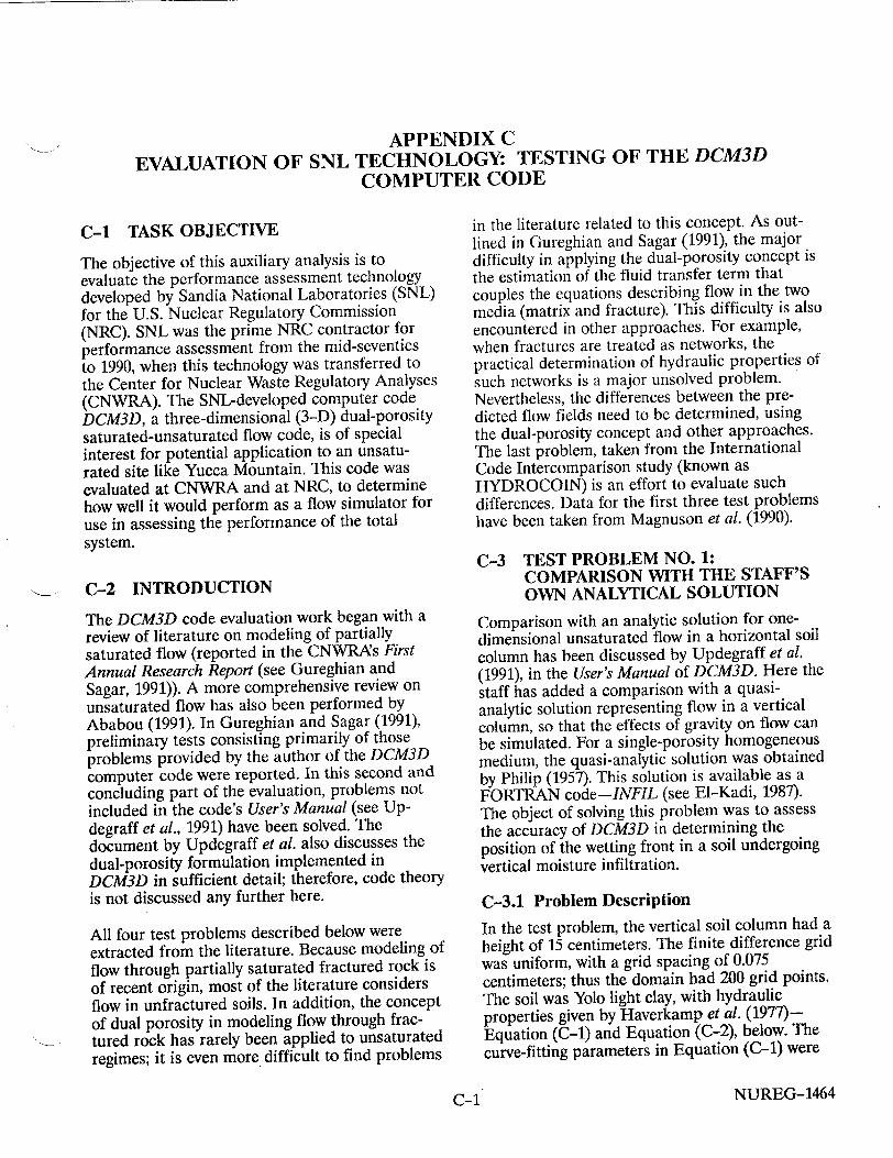
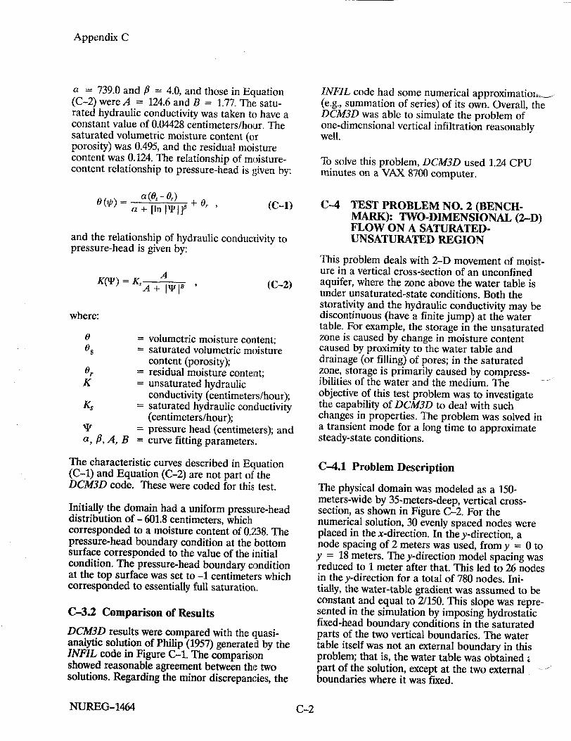
C-4.2 Comparison of Results
The PORFLO-3 results for this problem were taken from the report by Magnuson et al. (1990) where these results were compared with those from FEMWATER (Yeh and Ward, 1979). In Figure C-3, steady-state pressure-head contours from DCM3D are plotted. PORFLO-3 contours are not shown, as these are exactly the same as those for DCM3D, as shown in Figure C-3. Moisture-content profiles at a section 27.5 meters from the left boundary for DCM3D, and 30 meters for PORFLO-3, are compared in Figure C-4. The difference in locations of these sections is because of the two grid types used in the codes. DCM3D places the grid nodes in the middle of a cell, whereas PORFLO-3 places the cell boundary in the middle of the grid nodes. Despite this difference, the moisture contents compare favorably.
To solve this problem, DCM3D used 3.1 CPU minutes on a VAX 8700 computer.
C-5 TEST PROBLEM NO. 3 (BENCHMARK): SIMULATION OF JORNADA TRENCH EXPERIMENT
The Jornada trench experiment is located northeast of Las Cruces, New Mexico, on the New Mexico State University College Ranch. Funded by NRC, this experiment is expressly designed for collected data that can be used in model validation. In the following example, simulation results are not compared with the measured data, but, rather with simulations by another code. Hence, even though the experimental conditions are used as the input data, this test is termed a benchmark (rather than a validation) exercise. A more detailed description of this experiment was provided in the CNWRAs Quarterly Research Report (see Sagar and Wittmeyer, 1991).
The Jornada test problem is conceptualized as a vertical 2-D, multi-zone, unsaturated flow problem. Soil-hydraulic properties used in this test are based on those measured at the experimental site. This particular problem involves transient infiltration of water into an extremely dry, heterogeneous soil. Because of the initial dry conditions, the problem is highly nonlinear, and therefore is a good test for DCM3D.
NUREG-1464 C-4
Appendix C
35
30
2-5
'-20 Ec
Distance (mn)
Figure C-3 DCM3D pressure-head contour for a 2-D, saturated-unsaturated problem
35 a
30 KI
25
Figure C-4 Comparison of moisture contents from DCM3D and PORFL03, for Test Problem No. 2 mvmumo M .. . .
A•A
C-5
I U
WKrIJJL.t%"
Appendix C
C-5.1 Problem Description
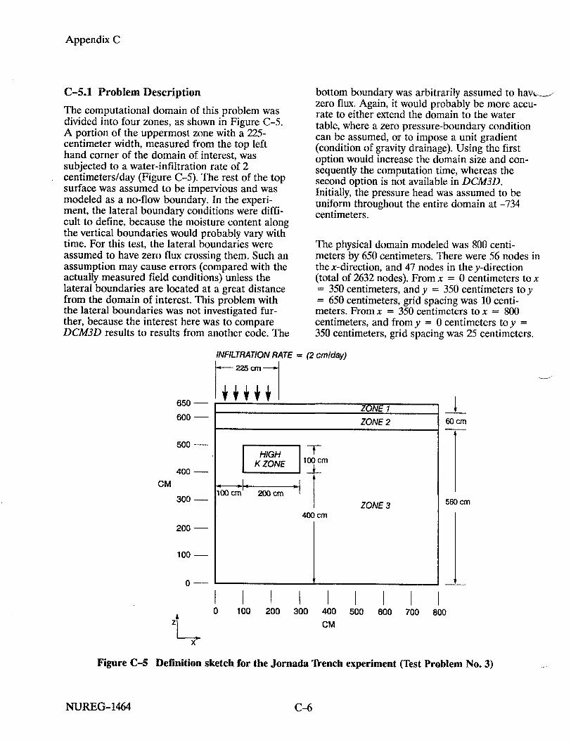
The computational domain of this problem was divided into four zones, as shown in Figure C-5. A portion of the uppermost zone with a 225centimeter width, measured from the top left hand corner of the domain of interest, was subjected to a water-infiltration rate of 2 centimeters/day (Figure C-5). The rest of the top surface was assumed to be impervious and was modeled as a no-flow boundary. In the experiment, the lateral boundary conditions were difficult to define, because the moisture content along the vertical boundaries would probably vary with time. For this test, the lateral boundaries were assumed to have zero flux crossing them. Such an assumption may cause errors (compared with the actually measured field conditions) unless the lateral boundaries are located at a great distance from the domain of interest. This problem with the lateral boundaries was not investigated further, because the interest here was to compare DCM3D results to results from another code. The
bottom boundary was arbitrarily assumed to have_. zero flux. Again, it would probably be more accurate to either extend the domain to the water table, where a zero pressure-boundary condition can be assumed, or to impose a unit gradient (condition of gravity drainage). Using the first option would increase the domain size and consequently the computation time, whereas the second option is not available in DCM3D. Initially, the pressure head was assumed to be uniform throughout the entire domain at -734 centimeters.
The physical domain modeled was 800 centimeters by 650 centimeters. There were 56 nodes in the x-direction, and 47 nodes in the y-direction (total of 2632 nodes). From x = 0 centimeters to x = 350 centimeters, and y = 350 centimeters toy = 650 centimeters, grid spacing was 10 centimeters. From x = 350 centimeters to x = 800 centimeters, and from y = 0 centimeters toy = 350 centimeters, grid spacing was 25 centimeters.
650
600
500
400
CM
300
200
100
0
x
INFILTRATION RATE = (2 cm/day)
225 cr-
0I I I I I I
100 200 300 400 500 600 700 800
CM
Figure C-5 Definition sketch for the Jornada Trench experiment (Test Problem No. 3)
NUREG-1464
ZONE 1 ZONE 2
K ZONE 1 0 cm
ZONE 3
400 cm
60 cm
560 cm
C-6

Appendix C
"The relationship of moisture content to pressurehead and the relationship of relative-permeability to moisture content are described by the van Genuchten (1980) equations as follows:
01(s0) (aTiy)+ 0T (C-5)
and
K, =F,11-[1-(ý - (C-6)
The variables are defined as follows:
0 = volumetric moisture content; Or = residual moisture content; 0, = saturated moisture content; S= pressure head; n = van Genuchten parameter; m = van Genuchten parameter
= (1 - 1/n); a = parameter; and Kr = relative hydraulic-conductivity.
The values of the input parameters for the four layers are given in Table C-1. The solver used was the LSODES, contained in ODEPACK (Hindmarsh, 1983). A relative convergence criterion of 1.0 X 10⁻⁵ and an absolute convergence criterion of 1.0 X 10⁻² were imposed.
C-5.2 Comparison of Results
Again, DCM3D results were compared to PORFLO-3 results taken from the report by Magnuson et al. (1990) in which PORFLO-3 results were compared with the results from FLASH (Baca and Magnuson, 1992). Earlier, Smyth et al. (1989) used the same data for a test of TRACER3D, a code developed at Los Alamos Laboratories by Travis (1984).
The simulations were run in 30-day durations. The saturations at 30 days after the start of the moisture infiltration are shown in Figure C-6. The previous comparison of PORFLO-3, FLASH, and TRACER3D results are shown in Figure C-7. All four codes showed a pronounced effect of the high permeability zone on moisture distribution. For this complex problem, results of all the codes differed somewhat from each other. Figure C-7 indicates large differences between results (e.g. in advance of the wetting front) from TRACER3D and the other codes. The DCM3D results were reasonably close to those from PORFLO-3 and FLASH.
DCM3D used 237 minutes of CPU time on a VAX 8700, while PORFLO-3 used 5.95 minutes of INEL Cray CPU time. For the same problem, the CPU times for TRACR3D and FLASH were reported to be 5.79 Hanford CRAY minutes and 16.8 INEL CRAY minutes, respectively. Unfortunately, because of different computing environments, these execution times were not directly comparable.
Table C-i Van Genuchten Soil Parameters
Zone 0s Or ar (cm- 1) n Ks
1 0.368 0.1020 0.0334 1.982 790.9
2 0.351 0.0985 0.0363 1.632 469.9
3 0.325 0.0859 0.0345 1.573 415.0
4 0.325 0.0859 0.0345 1.573 4150.0
NUREG-1464C-7

Appendix C
E .5 E 350 I
o 300 --. , . - .- I I
250 _
200 .6 •°°
ISO .4 DCM3D 15---------------------- C3
------. PORFLO-3 100
50
-- I 1. , 1 , f I ,, I , I I I I I 0 100 200 300 400 500 600
Distance (cm)
Figure C-6 Comparison of DCM3D and PORFLO-3 results (moisture contents) for the Jornada Trench experiment (Test Problem No. 3)
0 100 200 300 400 500
Distance (cm)
Figure C-7 Moisture content results for Test BT-2
600
NUREG-1464
CD
X-
C-8

Appendix C
Table C-2 Coordinates of the Numbered Points in Figure C-7 (from Prindle and Hopkins, 1990)
Coordinates (m) Coordinates (m)
Point x z Point x y
1 0.0 635.5 13 1000.0 224.0
2 0.0 608.7 14 1000.0 219.5
3 0.0 570.6 15 1000.0 130.3
4 0.0 440.5 16 1000.0 0.0
5 0.0 329.1 17 1000.5 530.4
6 0.0 324.6 18 1000.5 503.6
7 0.0 235.4 19 1000.5 465.5
8 0.0 0.0 20 1000.5 335.4
9 1000.0 530.4 21 1000.5 224.0
10 1000.0 503.6 22 1000.5 219.5
11 1000.0 465.5 23 1000.5 130.3
12 1000.0 465.5 24 1000.5 0.0
C-6 TEST PROBLEM NO. 4: 2-D FLOW THROUGH FRACTURED ROCK
The distinguishing feature of the DCM3D computer code is that it employs a dual-porosity conceptualization of the fractured porous medium, instead of an equivalent porous (singleporosity) medium or a fracture-network conceptualization. In the more common equivalent porous-medium approach, the characteristic curves for the rock matrix and the fractures are combined to form a composite characteristic curve. The composite curve assumes a rapid (with respect to the time scale of the flow being simulated) equilibration between the pressures of the fracture and matrix continua; and thus, the equilibration of pressure between the two continua is affected.
An important question is how different are the predicted flow fields for these two different conceptualizations. A convenient test case to explore this question was taken from the HYDROCOIN study. The test case was based on a flow field associated with unsaturated-fractured tuff (Prindle and Hopkins, 1990). The HYDROCOIN
test case was used here to examine the differences in the two conceptualizations, as well as to compare the DCM3D results with the HYDROCOIN results, to provide a measure of verification for DCM3D.
C-6.1 Problem Description
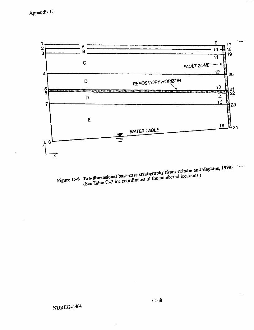
A complete description of the test case is provided in Prindle and Hopkins (1990). Only the information pertinent to the current simulations is provided here. The 2-D cross-section was comprised of five layers, with a uniform dip of 6 degrees at unit interfaces (Figure C-8). Additionally, a repository location and a fault zone were defined for the test case. Material properties for the various layers were reproduced from the Prindle and Hopkins report, in Table C-3.
The current simulations used modification 1, from the Prindle and Hopkins (1990) study. Modification 1 changed the original model description by not explicitly considering the fault zone and by modifying the rock properties, according to Table C-4. This modification was selected primarily because the beta parameter used for the van
NUREG-1464C-9
Appendix C
1 21 3
20
21 22
23
8 z
K
T8wo-dimensional base-case stratigraphY (from Prindle and Hopkins, 19 90)
(See Table C-2 for coordinates Of the numbered locationS.)
C-10
N-UREGIA464
24

Appendix C
Table C-3 Base Case Material Properties Used for the Hydrologic Units, as Depicted by Letters in Figure C-7 (from Prindle and Hopkins, 1990)
Matrix Properties
Hydraulic Conductivity Residual van Genuchten Parameters Unit Porosity (misec) Saturation Alpha (1/m) Beta
A 0.08 9.7 x 10⁻¹² 0.002 .00821 1.558 (.05 to .15) (1 X 10-13 to 5 x 10⁻¹⁰) (0. to .18) (.003 to .024) (1.3 to 2.4)
B 0.40 3.9 x 10⁻⁷ 0.100 .0015 6.872 (.20 to .70) (1 x 10⁻⁹ to 5 x 10⁻⁶) (0. to .15) (.001 to .031) (1.2 to 15.)
C 0.11 1.9 x 10⁻¹¹ 0.080 .00567 1.798 (.05 to .20) (1 x 10-13 to 5 x 10⁻¹⁰) (0. to .23) (.001 to .020) (1.2 to 2.5)
D 0.11 1.9 x 10⁻¹¹ 0.080 .00567 1.798 (.05 to .20) (1 x 10- 13 to 5 x 10⁻⁹) (0. to .32) (.001 to .020) (1.2 to 2.5)
Ev 0.46 2.7 x 10⁻⁷ 0.041 .0016 3.872 (.30 to .55) (1 x 10-13 to 5 x 10⁻⁶) (0. to .25) (.005 to .06) (1.3 to 7.0)
Ez 0.26 2.0 x 10⁻¹¹ 0.110 .00308 1.602 (.20 to .45) (1 X 10-14 to 5 x 10⁻¹⁰) (0. to .30) (.001 to .03) (1.2 to 3.5)
Individual Fracture Properties
Aperture Hydraulic Conductivity Density Unit (Microns) (misec) (No. Im 3) Porosity
A 6.74 3.8 x 10⁻⁵ 20 1.4 x 10⁻⁴
(5 X 10⁻⁷ to 5 x 10⁻³) (1 X 10⁻⁵ to .001)
B 27.0 6.1 x 10⁻⁴ 1 2.7 x 10⁻⁵
(5 x 10⁻⁶ to 5 x 10⁻²) (2 x 10⁻⁶ to 2 x 10.4)
C 5.13 2.2 x 10⁻⁵ 8 4.1 x 10⁻⁵ (5 x 10- 7 tol x 10-3) (2 x 10⁻⁶ to1 X 10-3)
D 4.55 1.7 x 10⁻⁵ 40 1.8 x 10⁻⁴
(1 x 10⁻⁷ to 1 X 10⁻³) (1 x 10⁻⁵ to 5 x 10⁻³)
Ev 15.5 2.0 x 10⁻⁴ 3 4.6 x 10⁻⁵ (2 x 10⁻⁶ to2 x 10-2) (5 x 10⁻⁶ to5 x 10-4)
Ez 15.5 2.0 x 10⁻⁴ 3 4.6 x 10⁻⁵
(2 x 10⁻⁶ to 2 x 10⁻²) (5 x 10⁻⁶ to 5 x 10⁻⁴)
NUJREG-1464C-11

Appendix C
Table C-3 (continued)
Bulk Fracture Properties
Bulk Hydraulic Conductivity Residual van Genuchten Parameters Unit Porosity (m/sec) Saturation Alpha(I/m) Beta
A 1.4 x 10⁻⁴ 5.3 x 10⁻⁹ 0.0395 1.285 4.23 (1 x 10⁻⁵ to .001) (5 x 10-12 to 5 x 10⁻⁶) (0. to .15) (.2 to 6.0) (1.2 to 7.0)
B 2.7 x 10⁻⁵ 1.6 x 10⁻⁸ 0.0395 1.285 4.23 (2 x 10⁻⁶ to 2 x 10⁻⁴) (1 x 10-11 to 1 x 10⁻⁵) (0. to .15) (.2 to 6.0) (1.2 to 7.0)
C 4.1 x 10⁻⁵ 9.0 x 10⁻¹⁰ 0.0395 1.285 4.23 (2 x 10⁻⁶ to 1 x 10⁻³) (1 X 10-12 to 1 x 10⁻⁶) (0. to .15) (.2 to 6.0) (1.2 to 7.0)
D 1.8 x 10⁻⁴ 3.1 x 10⁻⁹ 0.0395 1.285 4.23 (1 x 10⁻⁵ to 5 x 10⁻³) (1 X 10-12 to 1 X 10⁻⁶) (0. to .15) (.2 to 6.0) (1.2 to 7.0)
Ev 4.6 x 10⁻⁵ 9.2 x 10⁻⁹ 0.0395 1.285 4.23 (5 x 10⁻⁶ to 5 x 10⁻⁴) (1 x 10-11 to 1 x 10⁻⁵) (0. to .15) (.2 to 6.0) (1.2 to 7.0)
Ez 4.6 x 10⁻⁵ 9.2 x 10⁻⁹ 0.0395 1.285 4.23 (5 x 10⁻⁶ to 5 x 10⁻⁴) (1 X 10-11 to 1 x 10⁻⁵) (0. to .15) (.2 to 6.0) (1.2 to 7.01
Table C-4 Material Properties Used in Modification
(from Prindle and Hopkins, 1990)
Property Unit B Unit C Unit D
Km, b 1.0 X 10⁻⁷ 8.0 X 10⁻¹¹ 8.0 X 10⁻¹¹ am 0.010 0.015 0.015
#im 2.2 1.6 1.6 Kf,,b 3.6 x 10⁻⁶ 2.0 x 10⁻⁹ 3.1 x 10⁻⁹ nf 9.0 X 10⁻⁶ 9.0 x 10- 5 1.8 x 10⁻⁴
NUREG-1464 C-12

Appendix C
Genuchten equation was significantly lower (2.2 compared with 6.8) than the original value and was anticipated to lead to much shorter simulation times.
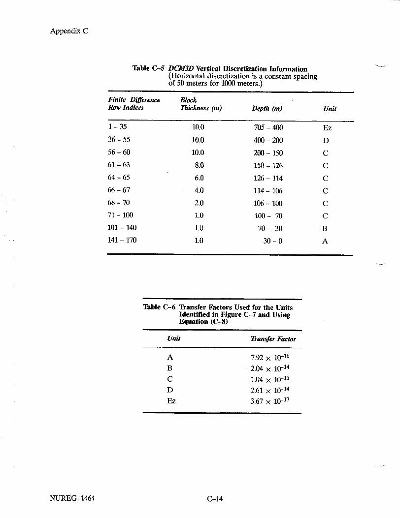
The finite difference grid for DCM3D was set up to provide the finest discretization in the vertical direction for the upper units (Table C-5) and a constant spacing in the horizontal direction. Rather than "stair-stepping" grid blocks at unit interfaces, the cross-sectional tilt was obtained by tilting gravity and increasing the depth to the water table by 100 meters (the depth to the water table was increased to decrease the affect of tilting the water-table boundary condition on the computational area of interest).
The tilting of gravity was considered to represent the problem description reasonably well, with the exception being near the side and bottom boundaries. Near the side boundaries, rather than a vertical boundary, the tilting of gravity causes the boundary to also appear slightly tilted. Near the bottom boundary, a significant flow is induced because of the tilting of gravity, which results in a gradient of 0.1. Despite these inaccuracies, the conceptualization was considered reasonable for examining flow diversion in the upper units (top 50 meters) and the spatial distribution of flow at the repository level (400 meters below the surface).
One additional parameter (the transfer term between matrix and fracture) was needed to perform the DCM3D simulations. The transfer term or factor, together with the gradient between the fracture and matrix controls the rate at which the fracture and matrix continua equilibrate. in the DCM3D User's Manual (Updegraff et al., 1991), this parameter is defined by the following equation:
(C-7)A =A,-T I
where:
A
Astransfer factor; matrix saturated permeability; fracture specific surface area per unit volume; and
= length parameter for gradient between fracture and matrix.
An attempt to determine the transfer factor in Equation (C-7), based on measurable quantities related to the fractures and matrix, was done by assuming that fractures were regularly spaced and planar and adopting a fracture-coating term. The fracture-coating term is used to represent a decrease (values less than 1) in transfer of water, resulting from a coating on the surface of the fracture, or an increase in transfer of water because of micro-fractures.
This conceptualization is represented by the following equation:
(C-8)Ar= 4Cn2 (k)-
where:
Ar = transfer factor, assuming regularspaced planar fractures;
C = fracture-coating term; n = number fractures per unit area; and S= saturated permeability of the matrix.
Equation C-8, the parametric values presented in Table C-3, and a coating factor of 0.5 were used to determine the transfer terms (see Table C-6).
One objective of this analysis was to compare the results, assuming a composite curve, with those obtained by assuming a dual-continuum approach. It was considered advantageous to implement a composite curve approach within DCM3D, so as to use one input file for both conceptualizations. Modifications to DCM3D were made such that it would accept the composite characteristic curve as input.
C-6.2 Comparison of Results
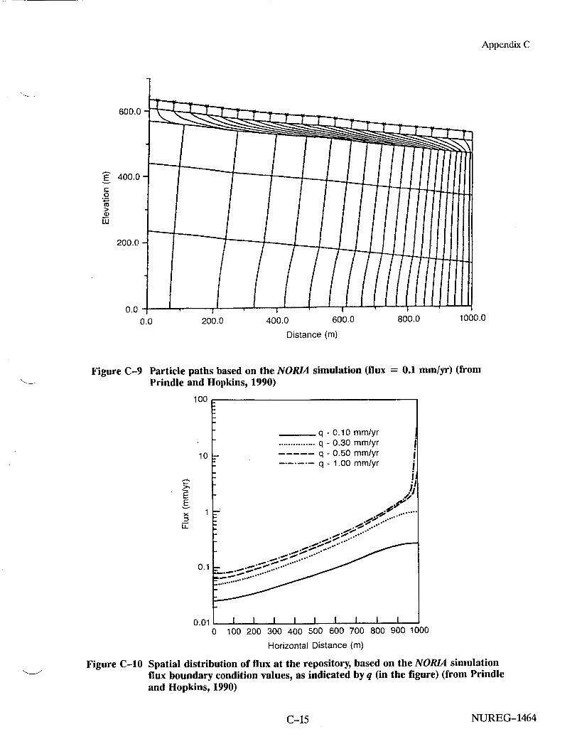
Performance measures used for this analysis were: (1) particle paths starting along the upper boundary; and (2) the spatial distribution of water flux at the repository level. The HYDROCOIN results are taken from Prindle and Hopkins (1990) and are presented in Figures C-9 and C-10. These simulation results were obtained with the computer program called NORMA (Bixler, 1985).
NUREG-1464C-13
Appendix C
Table C-5 DCM3D Vertical Discretization Information (Horizontal discretization is a constant spacing of 50 meters for 1000 meters.)
Finite Difference Block Row Indices Thickness (m) Depth (M) Unit
1-35 10.0 705-400 Ez
36-55 10.0 400-200 D
56-60 10.0 200-150 C
61-63 8.0 150-126 C
64-65 6.0 126-114 C
66-67 4.0 114-106 C
68-70 2.0 106-100 C
71-100 1.0 100- 70 C
101-140 1.0 70- 30 B
141-170 1.0 30-0 A
Table C-6 Transfer Factors Used for the Units Identified in Figure C-7 and Using Equation (C-8)
Unit Transfer Factor
A 7.92 x 10⁻¹⁶
B 2.04 x 10⁻¹⁴
C 1.04 x 10⁻¹⁵ D 2.61 x 10⁻¹⁴
Ez 3.67 x 10⁻¹⁷
NUREG-1464 C-14
200.0 400.0 600.0 800.0
Distance (m)
Particle paths based on the NORIA simulation (flux Prindle and Hopkins, 1990)
= 0.1 mm/yr) (from
100
q - 0.10 mm/yr ................ q - 0.30 mm/yr
10 q - 0.50 mm/yr ----q - 1.00 mm/yr
E E
2 ...,,, 0.1
0.01 I i I I I I I
0 100 200 300 400 500 600 700 800 900 1000
Horizontal Distance (m)
Figure C-10 Spatial distribution of flux at the repository, based on the NORIA simulation flux boundary condition values, as indicated by q (in the figure) (from Prindle and Hopkins, 1990)
NUREG-1464
Appendix C
600.0
E 400.0
200.0
0.0.
0.0
Figure C-9
1000.0
C-15
Appendix C
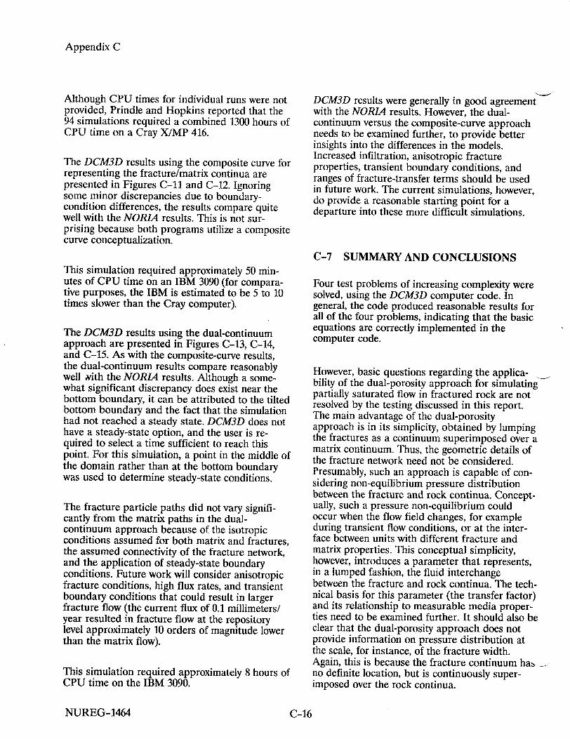
Although CPU times for individual runs were not provided, Prindle and Hopkins reported that the 94 simulations required a combined 1300 hours of CPU time on a Cray X/MP 416.
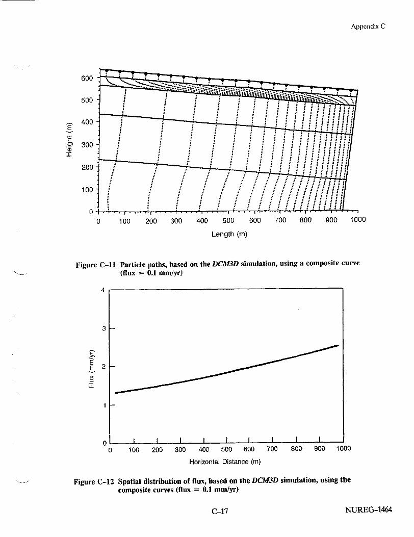
The DCM3D results using the composite curve for representing the fracture/matrix continua are presented in Figures C-11 and C-12. Ignoring some minor discrepancies due to boundarycondition differences, the results compare quite well with the NORM results. This is not surprising because both programs utilize a composite curve conceptualization.
This simulation required approximately 50 minutes of CPU time on an IBM 3090 (for comparative purposes, the IBM is estimated to be 5 to 10 times slower than the Cray computer).
The DCM3D results using the dual-continuum approach are presented in Figures C-13, C-14, and C-15. As with the composite-curve results, the dual-continuum results compare reasonably well 1vith the NORIA results. Although a somewhat significant discrepancy does exist near the bottom boundary, it can be attributed to the tilted bottom boundary and the fact that the simulation had not reached a steady state. DCM3D does not have a steady-state option, and the user is required to select a time sufficient to reach this point. For this simulation, a point in the middle of the domain rather than at the bottom boundary was used to determine steady-state conditions.
The fracture particle paths did not vary significantly from the matrix paths in the dualcontinuum approach because of the isotropic conditions assumed for both matrix and fractures, the assumed connectivity of the fracture network, and the application of steady-state boundary conditions. Future work will consider anisotropic fracture conditions, high flux rates, and transient boundary conditions that could result in larger fracture flow (the current flux of 0.1 millimeters/ year resulted in fracture flow at the repository level approximately 10 orders of magnitude lower than the matrix flow).
This simulation required approximately 8 hours of CPU time on the IBM 3090.
DCM3D results were generally in good agreement with the NORIA results. However, the dualcontinuum versus the composite-curve approach needs to be examined further, to provide better insights into the differences in the models. Increased infiltration, anisotropic fracture properties, transient boundary conditions, and ranges of fracture-transfer terms should be used in future work. The current simulations, however, do provide a reasonable starting point for a departure into these more difficult simulations.
C-7 SUMMARY AND CONCLUSIONS
Four test problems of increasing complexity were solved, using the DCM3D computer code. In general, the code produced reasonable results for all of the four problems, indicating that the basic equations are correctly implemented in the computer code.
However, basic questions regarding the applicability of the dual-porosity approach for simulating partially saturated flow in fractured rock are not resolved by the testing discussed in this report. The main advantage of the dual-porosity approach is in its simplicity, obtained by lumping the fractures as a continuum superimposed over a matrix continuum. Thus, the geometric details of the fracture network need not be considered. Presumably, such an approach is capable of considering non-equilibrium pressure distribution between the fracture and rock continua. Conceptually, such a pressure non-equilibrium could occur when the flow field changes, for example during transient flow conditions, or at the interface between units with different fracture and matrix properties. This conceptual simplicity, however, introduces a parameter that represents, in a lumped fashion, the fluid interchange between the fracture and rock continua. The technical basis for this parameter (the transfer factor) and its relationship to measurable media properties need to be examined further. It should also be clear that the dual-porosity approach does not provide information on pressure distribution at the scale, for instance, of the fracture width. Again, this is because the fracture continuum has no definite location, but is continuously superimposed over the rock continua.
NUREG-1464 C-16
Appendix C
0 100 200 300 400 500 600 700 800 900 1000
Length (m)
Figure C-II
4
3
E
0
Figure C-12
Particle paths, based on the DCM3D simulation, using a composite curve (flux = 0.1 mm/yr)
0 100 200 300 400 500 600 700 800 900 1000
Horizontal Distance (m)
Spatial distribution of flux, based on the DCM3D simulation, using the composite curves (flux = 0.1 mm/yr)
NUREG-1464
E
9M
600
500
400
300
200
100
0
C-17

Appendix C
600
500
400
300
200 /
100
OL 0
0 1
-Figure C-13
-' an
00 200 4uU - Length (in)
Particle paths in the matrix, based on the DCM3D simulations, using the
dual-porositY model (flux = 0.1 mm/yr)
5 4-,
600
500
400
3001
200 /
100
0 0
Figure C-14
100 200 300
1000500 600
Length (m)
Particle paths in the fracture, based on DCM3D simulations' using the
dual-POrosity model (flux =0.1 mm/y'
NUREG-1464
E
-c
1000

Appendix C
4
3 H
E E
2
0 100 200 300 400 500 600 700 800 900 1000
Horizontal Distance (m)
Figure C-15 Spatial distribution of flux in the matrix, based on the DCM3D simulation, using the dual-porosity model (flux = 0.1 mm/yr)
Similar problems are also attendant to other approaches to modeling partially saturated flow in fractured porous media. Use of a composite characteristic curve has the same disadvantage as the dual-porosity approach, in not distinguishing the distinct location and geometry of the fractures. In addition, this approach requires the assumption that locally (within a computational cell) the pressures in the fracture and the rock are instantaneously in equilibrium. However, computationally, the composite-curve approach is simpler and less time-consuming than the dualporosity approach, because only a single governing equation needs to be solved. The fracturenetwork type of modeling requires not only detailed definition of the fracture topology, but also definition of its characteristic curves. Therefore, not only are the data needs multiplied, but the computation times become large. It may be that a mixed approach is appropriate, where the large faults that could control the flow system to a significant spatial scale (of the order of hundreds of meters) are represented as separate entities in the model, whereas the small fractures
are dealt with as dual-porosity or composite curves.
As new users1 of the DCM3D code, the IPA Phase 2 staff had difficulty in setting up the test problems. Some of the problems and recommendations are as follows:
" There is a need for experimental investigations of fracture-matrix interaction, to provide insight into applicability of the dualporosity concept and the composite-curve approach.
" The idea of using an approach that combines features of the dual-porosity and fracturenetwork approaches should be investigated.
" The input structure, in general, is cumbersome; no comments are allowed, and the analyst has to input a great deal of
1The authors of this report often ran into trouble while setting up the test problems previously discussed. When called upon, Mr. C. David Updegraff, developer of the DCM3D computer code, was gracious in providing advice. His help is gratefully acknowledged.
NUREG-1464C-19
0(
Appendix C
inconsequential quantities. The input can certainly be improved to compress the input files and make these more readable.
"* The options for the medium characteristic curves are too limited; at least one option allowing the input of a characteristic curve in a table format should be added.
"* Only rectangular coordinates are allowed; it should be a relatively minor matter to add the cylindrical coordinates.
"* Steady-state option is not available, and this problem cannot be easily fixed.
"* It would be worthwhile to examine what modifications are required to implement a steady-state option and to make the input more user-friendly.
"* The manner in which the gravity is introduced in the model is confusing.
"* The switch from thermodynamic pressure to pressure head is not straightforward; it essentially requires fooling the code, and total hydraulic head can not be used as a dependent variable, at all.
C-8 REFERENCES
Ababou, R., 'Approaches to Large Scale Unsaturated Flow in Heterogeneous, Stratified, and Fractured Geologic Media," U.S. Nuclear Regulatory Commission, NUREG/CR-5743, August 1991. [Prepared by the Center for Nuclear Waste Regulatory Analyses.]
Baca, R.G. and S.O. Magnuson, "FLASH-A Finite Element Computer Code for Variably Saturated Flow," Idaho Falls, Idaho, Idaho National Engineering Laboratory, EGG-GEO10274, August 1992. [Prepared by EG&G, Inc., for the U.S. Department of Energy.]
Bixler, N.E, "NORIA-A Finite Element Computer Program for Analyzing Water, Vapor, and Energy Transport in Porous Media," Albuquerque, New Mexico, Sandia National Laboratory, SAND84-2057, August 1985. [Prepared for the U.S. Department of Energy.]
E1-Kadi, A.I, INFIL, Indianapolis, Indiana, Holcomb Research Institute/International Groundwater Modeling Center, June 1987. [Computer program]
Gureghian, A.B. and B. Sagar, "Evaluation of DCM3D-A Dual Continuum, 3-D Groundwater Flow Code for Unsaturated, Fractured, Porous Media," in Patrick, WC. (ed.), "Report on Research Activities for Calendar Year 1990," U.S. Nuclear Regulatory Commission, NUREG/CR5817 (vol. 1), December 1991. [Prepared by the Center for Nuclear Waste Regulatory Analyses.]
Haverkamp, R., M. Vanclin, J. Touma, P. J. Wierenga, and G. Vachaud, 'A Comparison of Numerical Simulation Models for OneDimensional Infiltration," Soil Science Society of America Journal, 41:285-294 [1977].
Hindmarsh, A.C., "ODEPAK: A Systematized Collection of ODE Solvers," in Stepleman, R.S., et al. (eds.), Scientific Computing, Amsterdam, North-Holland Publishing Co., pp. 55-64, 1983.
Huyakorn, P.S., J.B. Kool, and J.B. Robertson, "VAM2D--Variably Saturated Analysis Model in Two Dimensions," U.S. Nuclear Regulatory Commission, NUREG/CR-5352, May 1989. [Prepared by Hydro Geologic, Inc.]
Magnuson, S.O., R.G. Baca, and A. Jeff Sondrup, "Independent Verification and Benchmark Testing of the PORFLO-3 Computer Code (Version 1.0)," Idaho Falls, Idaho, Idaho National Engineering Laboratory, EGG-BG-9175, August 1990. [Prepared by EG&G, Inc., for the U.S. Department of Energy.]
Philip, J.R, "Numerical Solution of Equations of the Diffusion Type with Diffusivity ConcentrationDependent II," Australian Journal of Physics, 10:29-42 [1957].
Prindle, R.W and P. Hopkins, "On Conditions and Parameters Important to Model Sensitivity for Unsaturated Flow Through Layered Fractured Tough; Results of Analyses for HYDROCOIN Level 3, Case 2," Sandia National Laboratories, SAND89-0652, July 1990.
Runchal, A.K. and B. Sagar, "PORFLO-3: A Mathematical Model for Fluid Flow, Heat and Mass Transport in Variably Saturated Geologic
NUREG-1464 C-20

Appendix C
Media-User's Manual (Version 1.0)," Richland, Washington, Westinghouse Hanford Company, WHC-EP-0041, July 1989.
Sagar, B. and A.K. Runchal, "PORFLO-3: A Mathematical Model for Fluid Flow, Heat and Mass Transport in Variably Saturated Geologic Media-Theory and Numerical Methods (Version 1.0)," Richland, Washington, Westinghouse Hanford Company, WHC-EP-0042, March 1990.
Sagar, B. and G. Wittmeyer, "Phase 2 Interval Project: Las Cruces Trench Solute Transport Modeling study, Plot 2, Experiment A," in Patrick, WC. (ed.), Report on the Research Activities for the Quarter January 1 Through March 31, 1991, San Antonio, Texas, Center for Nuclear Waste Regulatory Analyses, CNWRA 91-01Q, November 1991.
Smyth, J.D., S.B. Yabusaki, and G.W Gee, "Infiltration Evaluation Methodology--Letter Report 3: Selected Tests of Infiltration Using Two-Dimensional Numerical Models," Richland,
Washington, Pacific Northwest Laboratory, July 1989.
Travis, B.J., "TRACER3D: A Model of Flow and Transport in Porous-Fractured Media," Los Alamos, New Mexico, Los Alamos National Laboratories, LA-9667-MS, May 1984. [Prepared for the U.S. Department of Energy.]
Updegraff, C.D., C.E. Lee, and D.P. Gallegos, "DCM3D: A Dual-Continuum, ThreeDimensional, Ground-Water Flow Code for Unsaturated, Fractured, Porous Media," U.S. Nuclear Regulatory Commission, NUREG/CR5536, February 1991.
Van Genuchten, M.T, 'A Closed-Form Equation for Predicting the Hydraulic Conductivity of Unsaturated Soils," Soil Science, 44:892-898 [1980].
Yeh, G.T, and D.S. Ward, "FEMWATER: A Finite-Element Model of Water Flow through SaturatedUnsaturated Porous Media," Oak Ridge, Terinessee, Oak Ridge National Laboratory, ORNL-5567, August 1979.
NUREG-1464C-21

APPENDIX D Kd APPROXIMATION TESTING
D-1 INTRODUCTION
The most widely accepted conceptualization for the release of radionuclides from a geologic repository for high-level radioactive waste (HLW) to the accessible environment involves ground water that flows through the repository, interacts with the radioactive waste, and carries the resulting dissolved and/or suspended contaminants to the accessible environment (10 CFR 60.2). In traveling along the path from the repository to the accessible environment, these radionuclides can interact with solids. These interactions can include precipitation/dissolution and sorption/desorption. This auxiliary analysis will focus on sorption/desorption reactions. When associated with the solid as results from sorption reactions, the radionuclide is immobile. The length of time the radionuclide is associated with the immobile solid phase versus the time the radionuclide spends in the flowing ground water affects the rate of radionuclide migration. The "more time spent on the solid, the more retarded is the movement of the radionuclide relative to the ground-water flow rate. The retardation of radionuclides by interactions with the geologic medium can limit the amount of radionuclides reaching the accessible environment in 10,000 years, as required by the Nuclear Regulatory Commission's regulation.1
Retardation is a process ascribed to dynamic systems. Chromatographic theory, however, states that, given certain assumptions, parameters measured in static systems can be used to calculate retardation in dynamic systems. Traditionally, static, batch experiments are performed in which
lCurrently, a revised set of standards specific to the Yucca Mountain site is being developed in accordance writh the provisions of the Energy Policy Act of 1992. The Energy Policy Act of 1992 (Public Law 102-486), approved October 24, 1992, directs NRC to promulgate a rule, modifying 10 CFR Part 60 of its regulations, so that these regulations are consistent with EPAs public health and safety standards for protection of the public from releases to the accessible environment from radioactive materials stored or disposed of at Yucca Mountain, Nevada, consistent with the findings and recommendations made by the National Academy of Sciences, to EPA, on issues relating to the environmental standards governing the Yucca Mountain repository. It is assumed that the revised EPA standards for the Yucca Mountain site will not be substantially different from those currently contained in 40 CFR Part 191, particularly as they pertain to the need to conduct a quantitative performance assessment as the means to estimate postclosure performance of the repository system.
ground water containing a radionuclide is brought into contact with solids expected to occur along the flowpath to the accessible environment. The radionuclide partitions itself between solid and liquid phases. After the experiment, the concentrations of radionuclide on the solid and in the liquid are measured. When sorption/desorption are the processes controlling radionuclide/solid interactions, the ratio of radionuclide concentration on the solid to that in the liquid is called the sorption coefficient, or Kd, and normally has units of milliliters per gram. The relationship of Kd to retardation is:
1-f Kd (D-1)
where o is the bulk density, 6 is the porosity, and Rf is the retardation factor, which is defined as the ratio of the velocity of the groundwater to that of the radionuclide. Freeze and Cherry (1979, p. 404) state that Equation (D-1) is valid when:
" The sorption reaction is fast and reversible; and
"* The sorption isotherm is linear.
A sorption isotherm is the locus of points describing the concentration of radionuclide on the solid as a function of its concentration in the liquid. When the isotherm is linear, Kd is constant (i.e., independent of radionuclide concentration in the liquid.)
D-2 BACKGROUND/DEFINITION OF ISSUES
The total-system performance assessment (TPA) computer code of the present NRC performance assessment effort uses the Kd approach in estimating retardation of radionuclides. The sources of the values of Kd used in the TPA computer code are Meijer (1990) and Thomas (1987). These Kds are based on batch sorption tests, supported in some cases by corresponding flow-through column experiments performed by investigators from the Los Alamos National Laboratory. The batch sorption tests use site-specific ground water
NUREG-1464
Appendix D
to which radionuclides have been added, and crushed solids expected to occur along the flowpath from the repository to the accessible environment.
In a system as complex as Yucca Mountain, it remains to be demonstrated that simplifications such as the Kd approach in estimating retardation are valid. This auxiliary analysis tests the requirement that the sorption isotherm needs to be linear to make Equation (D-1) valid. The method involves modeling sorption reactions in a one-dimensional flowing system. Two specific sorption reactions are ion exchange and surface complexation. This modeling exercise simulates ion exchange involving sodium and potassium. The reaction considered is:
K+ + NaX = KX + Na+ (D-2)
where X is the sorbing site on the solid. This simple system was chosen as a first attempt to investigate the effects of ion exchange on solute migration. Lacking thermodynamic data on site-specific components, this simple system can be viewed as an analog for the radionuclide-tuff reactions at Yucca Mountain. The computer code capable of simulating these processes is PHREEQM, for use in mixing cell flowtube simulations described by Appelo and Willemsen (1987). This code, an adaptation of PHREEQE (Parkhurst et al., 1990) can simulate speciation and mass-transfer processes, including precipitation, and dissolution, plus it can simulate ion exchange reactions, one-dimensional flow and transport, diffusion, and dispersion in a porous media. The reaction written above describes the situation where a solution containing potassium flows through a porous medium initially loaded with sodium. The potassium dissolved in the aqueous phase displaces sodium on the solid and this solute-solid interaction retards the movement of potassium down the column relative to that of water. One could also imagine that the potassium represents a radionuclide and X represents sorbing site on the tuff.
Investigators involved in the Yucca Mountain geochemical program perform batch sorption tests to determine an isotherm. If the isotherm is linear, a retardation factor is calculated. Sometimes, additional characterization may be performed to
establish the actual mechanism responsible foi the sorption. In this auxiliary analysis, however, the sorption mechanism is already known. Simulation of a flow-through experiment produces elution curves that are retarded relative to the flow of water. Thus, retardation factors can be determined. Finally, Kd values and sorption isotherms can be generated by characterizing the partitioning of the sorbing species for all points along the column at all times.
The mass-action equation corresponding to Equation (D-2) is:
[K+][NaI ' [K+ - [KNaXl (D-3)
where K is the equilibrium constant for the reaction and brackets represent activities. For this reaction, K is 5 (an arbitrary value in the database used by PHREEQM). For this study, accurate values for thermodynamic constants for specific reactions are not required, as only general relationships among parameters and their effects on solute migration are investigated. In compar" son, the exchange constant for the K+ - Na+ ion-exchange reaction involving clinoptilolite is 17.2 (Pabalan, 1991). If the reverse of Equation (D-2) is considered,
Na+ + KX -K+ +NaX , (D-4)
where the equilibrium constant is 1/5.
Vermeulen et al. (1987) subdivide sorption reactions into various types, depending on the shape of the isotherm. Isotherms that are convex up are termed favorable (e.g., Figure D-la) and those that are concave up are termed unfavorable (e.g., Figure D-lb). The terms favorable and unfavorable refer to the ability of a chromatographic process to separate species that are variably sorbed. A favorable sorption reaction would result in elution curves with constant-shaped fronts. These are also termed self-sharpening fronts. An unfavorable sorption reaction would result in elution curves with changing or spreading fronts. For an ion-exchange process, if the equilibrium constant is greater than 1, sorption processes favorable for chromatographic separation are present. If the equilibrium constant is less thart unfavorable conditions are present.
NUREG-1464 D-2

Appendix D
-o
0
S(a) 0
~0
r- (b)
0 t
Concentration of Radionuclide in Liquid
Figure D-1 Nonlinear isotherms ((1a) Favorable isotherm; (1b) Unfavorable isotherm.)
Some of the sorption isotherms using site-specific materials from Yucca Mountain are nonlinear (DOE, 1988; pp. 4-81-4-82). These isotherms have been fitted using a Freundlich formulation:
C, = KC7' , (D-5)
where Cs and C1 are concentrations on the solid and in the liquid, respectively, and K and n are empirical constants. When n is greater than 1, the isotherm is concave up, and when it is less than 1, it is convex up. For plutonium, n is 0.84 to 0.88, when YM-22 (welded tuff) is the solid substrate and 0.96 to 1.0, when YM-49 (partially zeolitized and vitric sample) is the solid. For strontium, cesium, barium, and europium, n ranges from 0.71 to 0.92, when the solid substrate is YM-22 (DOE, 1988; p. 4-82). The isotherm for these elements is linear when the solid is zeolitized.
By simulating flow-through experiments involving "ion exchange represented by Equations (D-2) and (D-4), both favorable and unfavorable elutions
are modeled. The significance of these types of elutions to performance assessment can then be better appreciated.
Simulations
Conceptually, the column is divided into cells. Initially, the chemical constituents in each cell are reacted to equilibrium. The possible reactions include precipitation, dissolution, speciation, and ion exchange. Mixing is then simulated between adjacent cells. The mixing can be caused by both dispersion and diffusion. However, in the present study, it was decided arbitrarily that only dispersion be included in the simulation. Following mixing, the solutions in each cell are moved to the next cell downstream and re-equilibrated. The solution added to the column is called the flushing solution. Its composition remains constant throughout the simulation. Before adding the flushing solution, the compositions of both liquid and solid in the column are defined. The parameters that are varied in this study are the relative
NUREG-1464D-3
Appendix D
concentrations of competing species, and concentration of the sorbing site or complex, X-.
The capability of a solid to sorb is commonly described in terms of cation-exchange capacity. The code, however, uses the concentration of the sorbing site, X- (in milliequivalents per litermeq/L), which is related to the cation exchange capacity by the relation:
CEC x 1000 X-(meq/L) = 100 X 0 (D-6)
Q
where CEC is the cation exchange capacity in meq per 100 grams soil, 0 is the porosity, and Q is the bulk density of the soil in kilograms per liter.
Porosity is an input in the simulation and must remain constant along the length of the column, to maintain the constancy of masses of solution moving from cell to cell. The simulations involve only saturated hydrologic conditions. Porosity in these simulations has been set at 0.3, which lies within the range of porosities found at Yucca Mountain (see DOE, 1988; p. 3-192).
In the PHREEQM code, mixing between adjacent cells is calculated using the relation:
f= DISP(i) + DISP(i + 1) + 4 x DM x DELTAT L(i) + L(i + 1) (L(i) + L(i + 1))2
(D-7)
where f is the mixing factor, DISP is the dispersivity in meters, L is the length of the cell in meters, i represents the cell number, DM is the diffusivity in square meters/second, DELTAT is the time for diffusion in seconds. The mixing factor is the percentage of a cell's dissolved contents that is transferred to an adjacent cell. Both upstream and downstream adjacent cells are involved in the mixing process. The code restricts f < 0.33 so that at least one-third of the original contents of a cell remain after a mixing simulation. All the factors on the right side of Equation (D-7) are inputs to the code. For this study, no diffusion is simulated, so the second term on the right side of Equation (D-7) is zero, and only the dispersion component
of spreading is considered. All the simulations this study have the same dispersivity.
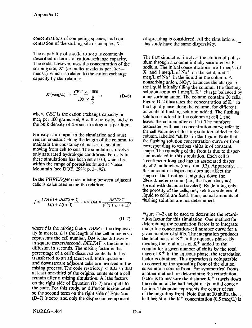
The first simulation involves the elution of potassium through a column initially saturated with sodium. The initial concentrations are 1 meq/L of X- and 1 meq/L of Na+ on the solid, and 1 meq/L of Na+ in the liquid in the column. A nonsorbing anion, NO3-, balances the charge in the liquid initially filling the column. The flushing solution contains 1 meq/L K+ charge balanced by a nonsorbing anion. The column contains 20 cells. Figure D-2 illustrates the concentration of K+ in the liquid phase along the column, for different amounts of flushing solution added. The flushing solution is added to the column at cell 1 and leaves the column after cell 20. The numbers associated with each concentration curve refer to the cell volumes of flushing solution added to the column, labelled "shifts" in the figure. Note that the flushing solution concentration curve or front corresponding to various shifts is of constant shape. The rounding of the front is due to dispersion modeled in this simulation. Each cell is 1-centimeter long and has an associated disper ity of 2 millimeters (thus, f = 0.2). Apparently, this amount of dispersion does not affect the shape of the front as it migrates down the 20-centimeter column (i.e., the front does not spread with distance traveled). By defining only the porosity of the cells, only relative volumes of liquid to solid are fixed. Thus, actual amounts of flushing solution are not determined.
Figure D-2 can be used to determine the retardation factor for this simulation. One method for determining the retardation factor is to integrate under the concentration-cell number curve for a given number of shifts. The integration produces the total mass of K+ in the aqueous phase. By dividing the total mass of K+ added to the column for a given number of shifts by the total mass of K+ in the aqueous phase, the retardation factor is obtained. This operation is comparable to converting the spreading front of the elution curve into a square front. For symmetrical fronts, another method for determining the retardation factor is to measure the distance K+ travels down the column at the half height of its initial concer tration. This point represents the center of ma, of the migrating front. Note that at 20 shifts, th.half height of the K+ concentration (0.5 meq/L) is
NUREG-1464 D--4

Appendix D
1 2 3 4 5 6 7 8 9 10 11 12 13 14 15 16 17 18 19 20
Cell NumberFlushing solution concentration versus cell number, flushing solution solute preferentially sorbed, equal starting concentrations of flushing solution solute, competing cation and sorbing site
in cell 10. Thus, at this point the water has traveled all the way through the column, but K+ has traveled only half the distance. Consequently, the retardation factor, Rf, is 2. From Equation (D-1), if e is assumed to be 2.5, the Kd is 0.12.
Each cell can be considered as a separate batch sorption test. The code calculates the partitioning of the ions between solid and liquid. Thus, it is possible to determine a Kd for K+ for each cell and each shift. Figure D-3 is a plot of Kd versus cell number for various shifts. The Kd values range from 0.6 to 0.12 and are not constant for a particular cell (space), but change with the number of shifts (time). For example, cell 6 has a Kd of 0.6 at 4 shifts and 0.12 at 15 shifts. It should be noted that K+ has reached cell 6 after only four shifts because of the dispersion where 20 percent of the dissolved contents of each cell is moved downstream per shift. Combined with information from Figure D-2, it is apparent that higher concentrations of K+ in a particular cell
correspond to the lower Kd value and vice versa. This observation provides an explanation for constant shape of the elution curve. Low concentrations lead high concentrations down the column. However, low concentrations correspond to high Kd values and so are slowed more than the high concentrations. The result is a front that maintains its steep concentration gradient.
The fact that this simulation produced a range of Kd values for particular cells raises an important issue, namely, what Kd value should be assigned to each cell? It is clear in this simulation that the appropriate Kcj for use in Equation (D-1) to determine retardation corresponds to the one measured at the highest flushing solution concentration. But, what if, as in the case of many of the radionuclides studied in the Yucca Mountain Project, only Kd values as a function of radionuclide concentration are determined for rockwater systems representing various locations in the repository block? Must not the radionuclide
NUREG-1464
1.0
0.9
0.8
0.7
0.6
0.5
0.4
0.3
0.2
0.1
0
CH
0
0 0
Figure D-2
D-5

Appendix D 0.7
0.6
0.5
E 0.4
0.3
0.2
01 2 3 4 5 6 7 8 9 10 11 12 13 14 15 16 17 18 19 20
Cell Number Figure D-3 Kd versus cell number for flow-through ion exchange simulation illustrated
in Figure D-2
concentration at each location also be known in order to assign the appropriate Kd value? The approach to modelling radionuclide migration in the Yucca Mountain Project is to assume that Kd values are a function only of space and not time (Meijer, 1992). With this approach, a Kd value is chosen that is conservative relative to all Kd values, no matter what radionuclide concentration is present. However, it must be noted that Equation (D-5), describing the relation of radionuclide concentration on the solid to that in the liquid, has no formulation to limit the radionuclide concentration in the liquid. This limit must be supplied by additional information, such as solubilities.
From Figure D-2, it is evident that the concentrations of K+ in a particular cell can vary from 0 to 1 meq/L depending on the number of shifts and the position of the cell. By plotting the concentration of K+ on the solid in milliequivalents per gram versus the concentration in the liquid for all cells and all shifts, the sorption isotherm
can be generated. Figure D-4 is such a plot. This isotherm is convex up, and thus produces a front of constant shape, which is consistent with the description of Vermuelen et al. (1987). The points on Figure D-4 could be fitted to a curve such as the Freundlich formulation (Equation (D-5)), but it is not necessary for this study.
Figure D-5 illustrates the effect of doubling the concentration of K+ in the flushing solution while keeping all other parameters the same as in the first simulation. Here, for 20 shifts, or cell volumes added, the front measured at half concentration, falls between cell 12 and 13. This is comparable to a Kd of 0.07. Figure D-6 shows Kd values versus cell number for this simulated elution. Unlike in Figure D-2, where the Kd values monotonically change from one extreme to the other for a given shift, these curves develop a bulge with more shifts. The bulge can be explained by rearranging Equation (D-3) to express Kid as:
NUREG-1464
S.. . . . ..................... .............. .............
I
, / I Shift 4
II Shift 6Shift 15-..Shift 20 ..................
a 0 ' ~/"
K! / /
It
B •;
D-6

Appendix D
0.14
E•
2
0 C
0.12
0.1
0.0.
0.0
0.0
0.0
0 0.1 0.2 0.3 0.4 0.5 0.6 0.7 0.8 0.9 1.0 1.1
Concentration (meq/mi) Thousandths
Figure D-4 Sorption isotherm calculated from flow-through ion exchange simulation illustrated in Figure D-3 showing favorable characteristics
2.5
2
0)0
cc5
CO 0
0 0
1.5
1
0.5
01 2 3. 4 5 6 7 8 9 10 11 12 13 14 15 16 17 18 19 20
Cell Number
Figure D-5 Flushing solution concentration versus cell number, flushing solution solute perferentially sorbed, effect of doubling starting concentration of flushing solution solute relative to competing cation and sorbing site concentrations
NUREG-1464
0 -O nm
8
6
4
I
2, I 1 i I
D-7
^

Appendix D
E
0.7
0.6
0.5
0.4
0.3
0.2
0.1
0
hift4 Shift 8 .........
- Shift 12 Shift 16 -. . Shift 20. Shift 24 ................
- - - - -
/i'
4• 4,
4,4,
4, 4, *4
4, S
1 I
I I
I I
I I
I I
I 4,
•,
I I I I I I I I I I I I
1 2 3 4 5 6 7 8 9 10 11 12 13 14 15 16 17 18 19 20
Cell Number
4, 4,
4,
Kd versus cell number for flow-through ion exchange simulation illustrated in Figure D-5
x INaXI [Na+]
(D-8)
where activities approximate concentrations. Since the equilibrium constant is fixed, the variation in Kd is caused by a variation in the concentrations of the sodium species. Figure D-7 shows the displacement of sodium on the solid by potassium in the flushing solution. As a result of the higher K+ concentration, more Na+ is displaced to the liquid in each cell downstream than was originally present (1 meqL in liquid and 1 meq/L on solid). A wave of Na develops with its crest increasing with the number of cell volumes added to the column. Thus, although the [NaX] varies smoothly from 0 to 1 meq/L down the column, the [Na +] goes through a maximum. This variation causes the bulge in the Kdj values.
The ion-exchange reaction represented by Equation (D-4) involves the migration of sodium
through a column initially saturated with potassium. With an equilibrium constant of 115, this simulation should result in the unfavorable condition of non-constant-shaped fronts. Figure D-8 illustrates the elution of 1 meq/L of Na+ in the flushing solution through a column having 1 meq/L for both KX on the solid and K+ in solution. The curves representing various shifts definitely are not of constant shape. The retardation factor calculated for shift 16 is approximately 1.6. Unlike the favorable condition (Figure D-2) where, with a retardation factor of 2, no flushing solution solute was exiting the column even after 24 shifts, here significant flushing solution solute passes through the column at 20 shifts. Dispersivity for both favorable and unfavorable simulations is the same (2 millimeters). This simulation demonstrates that, in addition to the retardation factor, the shape of the curve is also important. Thus, with regard to Yucca Mountain, for a given retardation factor, the amount of radionuclidF reachingthe accessible environment depends whether the ion exchange is favorable or not.
NUREG-1464
Figure D-6
[K] - Kd =K [K+1
It° I1•
D-8

Appendix D
2.5
2
1.5
1 2 3 4 5 6 7 8 9 10 11 12 13 14 15 16 17 18 19 20
Figure D-7 I
1 .1
0.9
0.8
-" 0.7
.S" 0.6
-U)
= 0.5 0 0.4
Cell Number
Concentration of competing cation versus cell number for flow-through ion exchange simulation illustrated in Figure D-5
0.3
0.2
0.1
01 2 3. 4 5 6 7 8 9 10 11 12 13 14 15 16 17 18 19 20
Cell Number
Figure D-8 Flushing solution concentration versus cell number, flushing solution solute perferentially desorbed, equal starting concentrations of flushing solution solute, competing cation and sorbing site
NUREG-1464
-.2_
0 0 -
0.5
0
D-9
Appendix D
Figure D-9 shows Kd versus cell number for this simulation. Again the Kd values are not constant for a given cell. This graph does not have the same shape as Figure D-3, where the Kj values ranged between two extremes, with a retardation factor appropriately calculated from one of the Kd extremes. Here, the retardation factor corresponds to an intermediate Kd value. Figure D-10 is the sodium isotherm for this simulation. The curve is concave up, consistent with the unfavorable condition as described by Vermuelen et al. (1987).
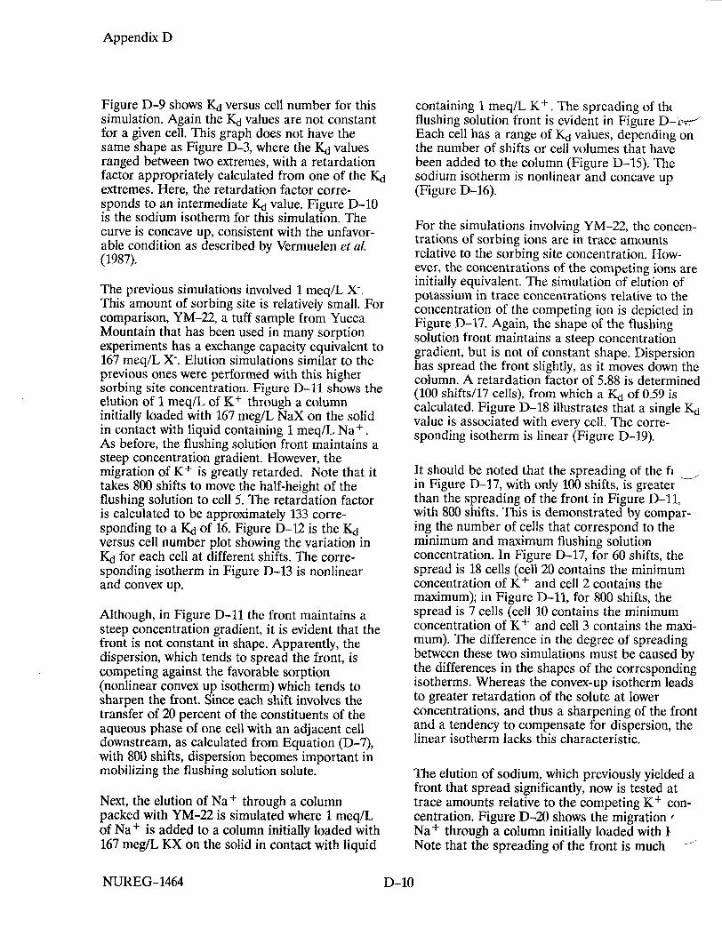
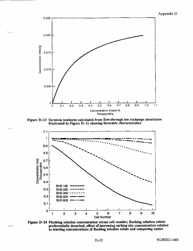
The previous simulations involved 1 meq/L X-. This amount of sorbing site is relatively small. For comparison, YM-22, a tuff sample from Yucca Mountain that has been used in many sorption experiments has a exchange capacity equivalent to 167 meq/L X-. Elution simulations similar to the previous ones were performed with this higher sorbing site concentration. Figure D-11 shows the elution of 1 meq/L of K+ through a column initially loaded with 167 meg/L NaX on the solid in contact with liquid containing 1 meq/L Na+. As before, the flushing solution front maintains a steep concentration gradient. However, the migration of K+ is greatly retarded. Note that it takes 800 shifts to move the half-height of the flushing solution to cell 5. The retardation factor is calculated to be approximately 133 corresponding to a Kd of 16. Figure D-12 is the Kd versus cell number plot showing the variation in Kd for each cell at different shifts. The corresponding isotherm in Figure D-13 is nonlinear and convex up.
Although, in Figure D-11 the front maintains a steep concentration gradient, it is evident that the front is not constant in shape. Apparently, the dispersion, which tends to spread the front, is competing against the favorable sorption (nonlinear convex up isotherm) which tends to sharpen the front. Since each shift involves the transfer of 20 percent of the constituents of the aqueous phase of one cell with an adjacent cell downstream, as calculated from Equation (D-7), with 800 shifts, dispersion becomes important in mobilizing the flushing solution solute.
Next, the elution of Na + through a column packed with YM-22 is simulated where 1 meq/L of Na + is added to a column initially loaded with 167 meg/L KX on the solid in contact with liquid
containing 1 meq/L K+. The spreading of tht flushing solution front is evident in Figure D-ir•-Each cell has a range of Kd values, depending on the number of shifts or cell volumes that have been added to the column (Figure D-15). The sodium isotherm is nonlinear and concave up (Figure D-16).
For the simulations involving YM-22, the concentrations of sorbing ions are in trace amounts relative to the sorbing site concentration. However, the concentrations of the competing ions are initially equivalent. The simulation of elution of potassium in trace concentrations relative to the concentration of the competing ion is depicted in Figure D-17. Again, the shape of the flushing solution front maintains a steep concentration gradient, but is not of constant shape. Dispersion has spread the front slightly, as it moves down the column. A retardation factor of 5.88 is determined (100 shifts/17 cells), from which a Kd of 0.59 is calculated. Figure D-18 illustrates that a single K, value is associated with every cell. The corresponding isotherm is linear (Figure D-19).
It should be noted that the spreading of the fi in Figure D-17, with only 100 shifts, is greater than the spreading of the front in Figure D-11, with 800 shifts. This is demonstrated by comparing the number of cells that correspond to the minimum and maximum flushing solution concentration. In Figure D-17, for 60 shifts, the spread is 18 cells (cell 20 contains the minimum concentration of K+ and cell 2 contains the maximum); in Figure D-11, for 800 shifts, the spread is 7 cells (cell 10 contains the minimum concentration of K+ and cell 3 contains the maximum). The difference in the degree of spreading between these two simulations must be caused by the differences in the shapes of the corresponding isotherms. Whereas the convex-up isotherm leads to greater retardation of the solute at lower concentrations, and thus a sharpening of the front and a tendency to compensate for dispersion, the linear isotherm lacks this characteristic.
The elution of sodium, which previously yielded a front that spread significantly, now is tested at trace amounts relative to the competing K+ concentration. Figure D-20 shows the migration Na+ through a column initially loaded with I Note that the spreading of the front is much
NUREG-1464 D-10

Appendix D
1 2 3 4 5 6 7 8 9 10 11 12 13 14 15 16 17 18 19 20
Cell Number
Figure D-9 1
0.14
0.12
0.10
'a
E3,
~00.08
0.06
0.04
0.02
Kd versus cell n Figure D-8
number for flow-through ion exchange simulation illustrated
0 0.1 0.2 0.3 0.4 0.5 0.6 0.7 0.8 0.9 1.0 1.1
Concentration (meq/ml) Thousandths
Figure D-10 Sorption isotherm calculated from flow-through ion exchange simulation illustrated in Figure D-8 showing unfavorable characteristics
NUREG-1464
0.13
0.12
0.11
0.1
0.09
S0.08 E "- 0.07
0.06
0.05
0.04
0.03
0.02
D-11

Appendix D
1.1
0.9
0.8
0.7
0.6
0.5
0.4
0.3
0.2
0.1
0
Figure D-1I
110
100 "
90
80 -
-o
70
60
50
40
30 "
20 [ 10
Figure D-12
Flushing solution concentration versus cell number, flushing solution solute preferentially sorbed, effect of increasing sorbing site concentration relative to starting concentrations of flushing solution solute and competing cation
I /
-I I
-I
iI I I
Shift 100 Shift 200 .... Shift 400 .......... Shift 600 Shift 800
I Il I I
1 2 3 4 5 6 7 8 9 10
Cell Number
Kd versus cell number for flow-through ion exchange simulation illustrated in Figure D-11
NUREG-1464
0
CO C-) C:
0 0
C')
0
I-
Shift 100 - \ \ Shift 200 -...
* Shift 400 ........... - Shift 600
"Shift 800
-. * \ \
I . \. .
2 3 4 5 6 7 8 9 10
Cell Number
D-12
= m 1 I ISI | I I
=
Appendix D
0 0.1 0.2 0.3 0.4 0.5 0.6 0.7 0.8 0.9 1.0 1.1
Figure D-13
1.1
11-
0.9 [
0.8 F-
6c 0.7
S0.6
.U) G 0: 0.5 o g
0 (j 0.4
0.3
0.2
0.1
0
F
4. 4.
4. 4.
4.
4. 4. 4.
Concentration (meq/ml) Thousandths
Sorption isotherm calculated from flow-through ion exchange simulation illustrated in Figure D-11 showing favorable characteristics
,t. .. .
%4.
Shift 100 Shift 200 Shift 400 ------Shift 600 Shift 800
I I I I I I
1 2 3 4 5 6 Cell Number
7 8 9 10
Figure D-14 Flushing solution concentration versus cell number, flushing solution solute preferentially desorbed, effect of increasing sorbing site concentration relative to starting concentrations of flushing solution solute and competing cation
NUREG-1464
0.025
0) 0� 0) E C 0
C a) C., C 0 0
III i . m m
I-_
D-13

Appendix D
4
3.5
3
E *0
2.5
2
1.51 2 3 4 5 6 7 8 9 10
Cell Number
Figure D-15
3.5
Kd versus cell number for flow-through ion exchange simulation illustrated in Figure D-14
3.0 H-
2.5 h-
__2.0
-2 o - 1.5
0
1.0
0.5 k-
0
Figure D-16
0 0.1 0.2 0.3 0.4 0.5 0.6 0.7 0.8 0.9 1.0 1.1Concentration (meq/ml)
Thousandths
Sorption isotherm calculated from flow-through ion exchange simulation illustrated in Figure D-14 showing unfavorable characteristics
NUREG-1464
.....................
%, -.............-......
-S.
S. -S. - -
Shift 100 Shift 200 .... Shift 400 ........... Shift 600 Shift 800
a I I I I
I I I I I I I I I I I
I I I I I I
D-14

Appendix D
0.03
0.025
0.02
0.015
0.01
0.005
1 2 3 4 5 6 7 8 9 10 11 1,
Cell Number
2 13 14 15 16 17 18 19 20
Figure D-17
1.1
0.9
0.8
Cr 0.7
8 0.6
5 0.5 U.!
O 0.4 C
0.3
0.2
0.1
0
Flushing solution concentration versus cell number, flushing solution solute preferentially sorbed, trace starting concentration of flushing solution solute, relative to competing cation and sorbing site concentrations
1 2 3 4 5 6 7 8 9 10 11 12 13 14 15 16 17 18 19 20
Cell Number
Figure D-18 Kd versus cell number for flow-through ion exchange simulation illustrated in Figure D-17
NUREG-1464
II 1 _ 1 I I I I I I I I I I
Shifts 20, 40, 60, 80 and 100
E Vý
0
D-15

Appendix D
0.7
0.6
0.5
0.4
0.3
0.2
0.1
00 0.1 -0.2 0.3 0.4 0.5 0.6 0.7 0.8 0.9
Concentration (meq/ml) Millionths
Figure D-19
1.1
0.9
0.8
C- 0.7
5 0.6 E0 0.5
0 0.4
0.3
0.2
0.1
0
Figure D-20
Sorption isotherm calculated from flow-through ion exchange simulation illustrated in Figure D-17 showing linear behavior
1 2 3. 4 5 6 7 8 9 10 11 12 13 14 15 16 17 18 19 20
Cell Number
Flushing solution concentration versus cell number, flushing solution solute preferentially desorbed, trace starting concentration of flushing solution solute, relative to competing cation and sorbing site concentrations
NUREG-1464
E
0
.C
0
1 1.1
D-16
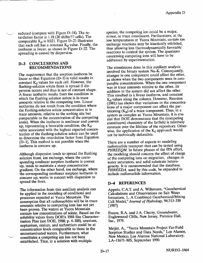
Appendix D
reduced (compare with Figure D-14). The retardation factor is 1.18 (20 shifts/17 cells). The comparable Kd is 0.021. Figure D-21 illustrates that each cell has a constant Kd value. Finally, the isotherm is linear, as shown in Figure D-22. The spreading is caused by dispersion.
D-3 CONCLUSIONS AND RECOMMENDATIONS
The requirement that the sorption isotherm be linear so that Equation (D-l) is valid results in constant Kd values for each cell. However, the flushing-solution solute front is spread if dispersion occurs and thus is not of constant shape. A linear isotherm results from the condition in which the flushing solution solute is in trace amounts relative to the competing ions. Linear isotherms do not result from the condition where the flushing-solution solute concentration is in trace amounts, relative to the sorbing site but comparable to the concentration of the competing ion(s). When the isotherm is nonlinear and convex up, representing a favorable condition, the Kd value associated with the highest expected concentration of the flushing-solution solute can be used to determine the retardation factor from Equation (D-1). This method is not possible when the isotherm is concave up.
Although dispersion tends to spread the flushing solution front, ion exchange, where the corresponding nonlinear sorption isotherm is convex up, tends to maintain a steep concentration gradient. On the other hand, ion exchange, where the corresponding nonlinear sorption isotherm is concave up, works in concert with dispersion to spread the front.
The information from this auxiliary analysis can be applied to the modeling of conditions and processes expected at Yucca Mountain. The assumption that all radionuclides will be in trace amounts relative to competing ions has not yet been proven. The waters at Yucca Mountain contain low concentrations of solute. Based on the solubility values from DOE's 1988 Site Characterization Plan (see DOE, 1988; p. 4-100), uranium, neptunium, cesium, and technetium could be at concentration levels comparable to those in the uncontaminated waters. Furthermore, what "constitutes a competing ion has not been established. Thus, in a solution with multiple
species, the competing ion could be a major, minor, or trace constituent. Furthermore, at the low temperatures at Yucca Mountain, certain ion exchange reactions may be kinetically inhibited, thus allowing less thermodynamically favorable reactions to control the system. The questions concerning competing ions will have to be addressed by experimentation.
The simulations done in this auxiliary analysis involved the binary system Na-K. Consequently, changes in one component could affect the other, as shown when the two components were in comparable concentrations. When the one component was in trace amounts relative to the other, its addition to the system did not affect the other. This resulted in a linear isotherm, and constant Kd values along the column. However, Reardon (1981) has shown that variations in the concentrations of a major component can affect the partitioning (Kd) of a trace component. Thus, in a system as complex as Yucca Mountain, it is crucial that DOE demonstrate that the (competing constituent) chemistry of the farfield is relatively constant over the lifetime of the repository. Otherwise, the application of the Kd approach would not be technically defensible.
There are a number of aspects to modeling radionuclide transport that can be tested using PHREEQM. In future phases of the IPA effort, the modeling should concern the effect of charge of the competing ions on migration, changes in water saturation, and solid substrate heterogeneity. It is recommended that the database, PHREEDA, used by this code, be expanded to include radionuclide information.
D-4 REFERENCES
Appelo, C.A.T and A. Willemsen, "Geochemical Calculations and Observations on Salt Water Intrusions, I., A Combined Geochemical/Mixing Cell Model," Journal of Hydrology, 94:313-330 [1987].
Freeze, R.A. and J.A. Cherry, Groundwater, Englewoood Cliffs, New Jersey, Prentice Hall, Inc., 1979.
Meijer, A., "Yucca Mountain Project Far-Field Sorption Studies and Data Needs," Los Alamos, New Mexico, Los Alamos National Laboratory, LA-11671-MS, September 1990.
NUREG-1464D-17

Appendix D
0.03
0.025 Shifts 4, 8, 12, 16, 20 and 24
0.02
o0.015
0.01
0.005
0 I I I 1 2 3 4 5 6 7 8 9 10 11 12 13 14 15 16 17 18 19 20
Cell Number
Figure D-21 Kd versus cell number for flow-through ion exchange simulation illustrated in Figure D-20
0.030
0.025
(D 0~
oct -o •=
0
0
0.020
0.015
0.010
0.005
0
Figure D-22
0 0.1 0.2 0.3 0.4 0.5 0.6 0.7 0.8 0.9 1.0 1.1
Concentration (meq/mt,) Millionths
Sorption isotherm calculated from flow-through ion exchange simulation illustrated in Figure D-20 showing linear behavior
NUREG-1464 D-18

Appendix D
Meijer, A., 'A Strategy for the Derivation and Use of Sorption Coefficients in Performance Assessment Calculations for the Yucca Mountain Site," Proceedings of the DOE/Yucca Mountain Site Characterization Project Radionuclide Adsorption Workshop, September 11-12, 1990, Los Alamos, New Mexico, Los Alamos National Laboratory, LA-12325-C, August 1992.
Pabalan, R.T, "Nonideality Effects on the Ion Exchange Behavior of the Zeolite Mineral Clinoptilolite," in Abrajano, T, Jr. and L.H. Johnson (eds.), Scientific Basis for Nuclear Waste Management XIV Materials Research Society Symposium Proceedings, 212:559-567 [1991].
Parkhurst, D.L., D.C. Thorstenson, and L.N. Plummer, "PHREEQE: A Computer Program for Geochemical Calculations," U.S. Geological Survey, Water Research Investigations Report, WRI-80-96, August 1990.
Plummer, L.N., et al., "Dissolution of AragoniteStrontionite Solid Solutions in Nonstoichiometric Sr(HCO 3)2-Ca(HCO 3)2-CO 2-H 20 Solutions," Geochimica et Cosmochimica Acta, 56:3045-3072 [1992].
Reardon, E.J., "Kd's--Can They Be Used to Describe Reversible Ion Sorption Reactions in
Contaminant Migration?," Groundwater, 19:279-286 [1981].
Thomas, K., "Summary of Sorption Measurements Performed with Yucca Mountain, Nevada, Tuff Samples and Water from Well J-13," Los Alamos, New Mexico, Los Alamos National Laboratory, LA-10960-MS, December 1987.
U.S. Department of Energy, "Site Characterization Plan, Yucca Mountain Site, Nevada Research and Development Area, Nevada," Nevada Operations Office/Yucca Mountain Project Office, Nevada, DOE/RW-0199, 9 vols., December 1988.
U.S. Nuclear Regulatory Commission, "Site Characterization Analysis of the Department of Energy's Site Characterization Plan, Yucca Mountain Site, Nevada," Office of Nuclear Material Safety and Safeguards, NUREG-1347, October 1989.
Vermeulen, T, et aL, 'Adsorption and Ion Exchange (Section 16)" in Perry, R.H., D.W Green, and J.O. Maloney (eds.), Perry's Handbook of Chemical Engineering (Sixth Edition), New York, McGraw-Hill, 1987.
NUREG-1464D-19
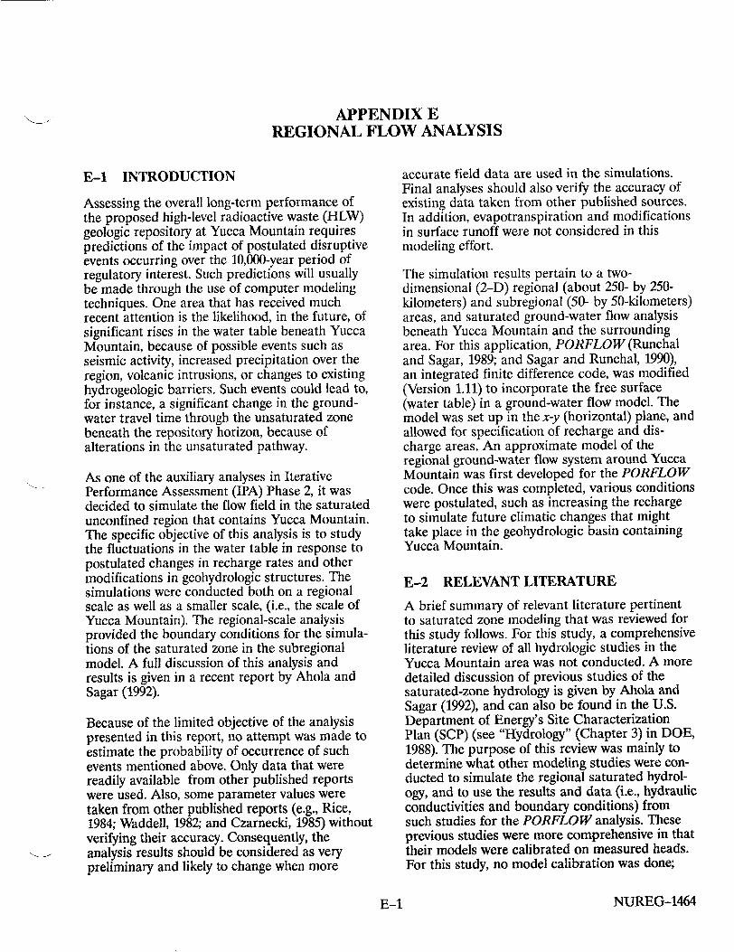
APPENDIX E REGIONAL FLOW ANALYSIS
E-1 INTRODUCTION
Assessing the overall long-term performance of the proposed high-level radioactive waste (HLW) geologic repository at Yucca Mountain requires predictions of the impact of postulated disruptive events occurring over the 10,000-year period of regulatory interest. Such predictions will usually be made through the use of computer modeling techniques. One area that has received much recent attention is the likelihood, in the future, of significant rises in the water table beneath Yucca Mountain, because of possible events such as seismic activity, increased precipitation over the region, volcanic intrusions, or changes to existing hydrogeologic barriers. Such events could lead to, for instance, a significant change in the groundwater travel time through the unsaturated zone beneath the repository horizon, because of alterations in the unsaturated pathway.
As one of the auxiliary analyses in Iterative Performance Assessment (IPA) Phase 2, it was decided to simulate the flow field in the saturated unconfined region that contains Yucca Mountain. The specific objective of this analysis is to study the fluctuations in the water table in response to postulated changes in recharge rates and other modifications in geohydrologic structures. The simulations were conducted both on a regional scale as well as a smaller scale, (i.e., the scale of Yucca Mountain). The regional-scale analysis provided the boundary conditions for the simulations of the saturated zone in the subregional model. A full discussion of this analysis and results is given in a recent report by Ahola and Sagar (1992).
Because of the limited objective of the analysis presented in this report, no attempt was made to estimate the probability of occurrence of such events mentioned above. Only data that were readily available from other published reports were used. Also, some parameter values were taken from other published reports (e.g., Rice, 1984; Waddell, 1982; and Czarnecki, 1985) without verifying their accuracy. Consequently, the analysis results should be considered as very preliminary and likely to change when more
accurate field data are used in the simulations. Final analyses should also verify the accuracy of existing data taken from other published sources. In addition, evapotranspiration and modifications in surface runoff were not considered in this modeling effort.
The simulation results pertain to a twodimensional (2-D) regional (about 250- by 250kilometers) and subregional (50- by 50-kilometers) areas, and saturated ground-water flow analysis beneath Yucca Mountain and the surrounding area. For this application, PORFLOW (Runchal and Sagar, 1989; and Sagar and Runchal, 1990), an integrated finite difference code, was modified (Version 1.11) to incorporate the free surface (water table) in a ground-water flow model. The model was set up in the x-y (horizontal) plane, and allowed for specification of recharge and discharge areas. An approximate model of the regional ground-water flow system around Yucca Mountain was first developed for the PORFLOW code. Once this was completed, various conditions were postulated, such as increasing the recharge to simulate future climatic changes that might take place in the geohydrologic basin containing Yucca Mountain.
E-2 RELEVANT LITERATURE
A brief summary of relevant literature pertinent to saturated zone modeling that was reviewed for this study follows. For this study, a comprehensive literature review of all hydrologic studies in the Yucca Mountain area was not conducted. A more detailed discussion of previous studies of the saturated-zone hydrology is given by Ahola and Sagar (1992), and can also be found in the U.S. Department of Energy's Site Characterization Plan (SCP) (see "Hydrology" (Chapter 3) in DOE, 1988). The purpose of this review was mainly to determine what other modeling studies were conducted to simulate the regional saturated hydrology, and to use the results and data (i.e., hydraulic conductivities and boundary conditions) from such studies for the PORFLOW analysis. These previous studies were more comprehensive in that their models were calibrated on measured heads. For this study, no model calibration was done;
NUREG-1464E-1
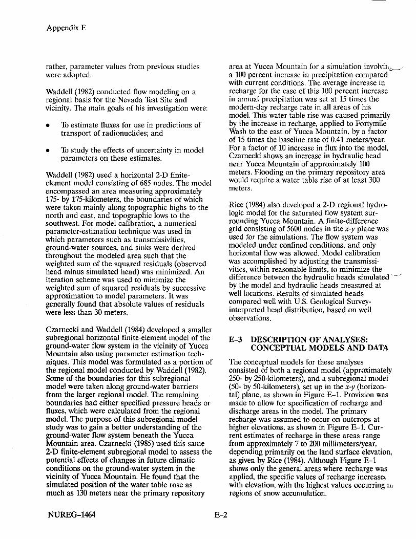
Appendix E
rather, parameter values from previous studies were adopted.
Waddell (1982) conducted flow modeling on a regional basis for the Nevada Test Site and vicinity. The main goals of his investigation were:
" To estimate fluxes for use in predictions of transport of radionuclides; and
" To study the effects of uncertainty in model parameters on these estimates.
Waddell (1982) used a horizontal 2-D finiteelement model consisting of 685 nodes. The model encompassed an area measuring approximately 175- by 175-kilometers, the boundaries of which were taken mainly along topographic highs to the north and east, and topographic lows to the southwest. For model calibration, a numerical parameter-estimation technique was used in which parameters such as transmissivities, ground-water sources, and sinks were derived throughout the modeled area such that the weighted sum of the squared residuals (observed head minus simulated head) was minimized. An iteration scheme was used to minimize the weighted sum of squared residuals by successive approximation to model parameters. It was generally found that absolute values of residuals were less than 30 meters.
Czarnecki and Waddell (1984) developed a smaller subregional horizontal finite-element model of the ground-water flow system in the vicinity of Yucca Mountain also using parameter estimation techniques. This model was formulated as a portion of the regional model conducted by Waddell (1982). Some of the boundaries for this subregional model were taken along ground-water barriers from the larger regional model. The remaining boundaries had either specified pressure heads or fluxes, which were calculated from the regional model. The purpose of this subregional model study was to gain a better understanding of the ground-water flow system beneath the Yucca Mountain area. Czarnecki (1985) used this same 2-D finite-element subregional model to assess the potential effects of changes in future climatic conditions on the ground-water system in the vicinity of Yucca Mountain. He found that the simulated position of the water table rose as much as 130 meters near the primary repository
area at Yucca Mountain for a simulation involvir,,._.• a 100 percent increase in precipitation compared with current conditions. The average increase in recharge for the case of this 100 percent increase in annual precipitation was set at 15 times the modern-day recharge rate in all areas of his model. This water table rise was caused primarily by the increase in recharge, applied to Fortymile Wash to the east of Yucca Mountain, by a factor of 15 times the baseline rate of 0.41 meters/year. For a factor of 10 increase in flux into the model, Czarnecki shows an increase in hydraulic head near Yucca Mountain of approximately 100 meters. Flooding on the primary repository area would require a water table rise of at least 300 meters.
Rice (1984) also developed a 2-D regional hydrologic model for the saturated flow system surrounding Yucca Mountain. A finite-difference grid consisting of 5600 nodes in the x-y plane was used for the simulations. The flow system was modeled under confined conditions, and only horizontal flow was allowed. Model calibration was accomplished by adjusting the transmissivities, within reasonable limits, to minimize the difference between the hydraulic heads simulated by the model and hydraulic heads measured at well locations. Results of simulated heads compared well with U.S. Geological Surveyinterpreted head distribution, based on well observations.
E-3 DESCRIPTION OF ANALYSES: CONCEPTUAL MODELS AND DATA
The conceptual models for these analyses consisted of both a regional model (approximately 250- by 250-kilometers), and a subregional model (50- by 50-kilometers), set up in the x-y (horizontal) plane, as shown in Figure E-1. Provision was made to allow for specification of recharge and discharge areas in the model. The primary recharge was assumed to occur on outcrops at higher elevations, as shown in Figure E-1. Current estimates of recharge in these areas range from approximately 7 to 200 millimeters/year, depending primarily on the land surface elevation, as given by Rice (1984). Although Figure E-1 shows only the general areas where recharge was applied, the specific values of recharge increaser with elevation, with the highest values occurring it, regions of snow accumulation.
NUREG-1464 E-2
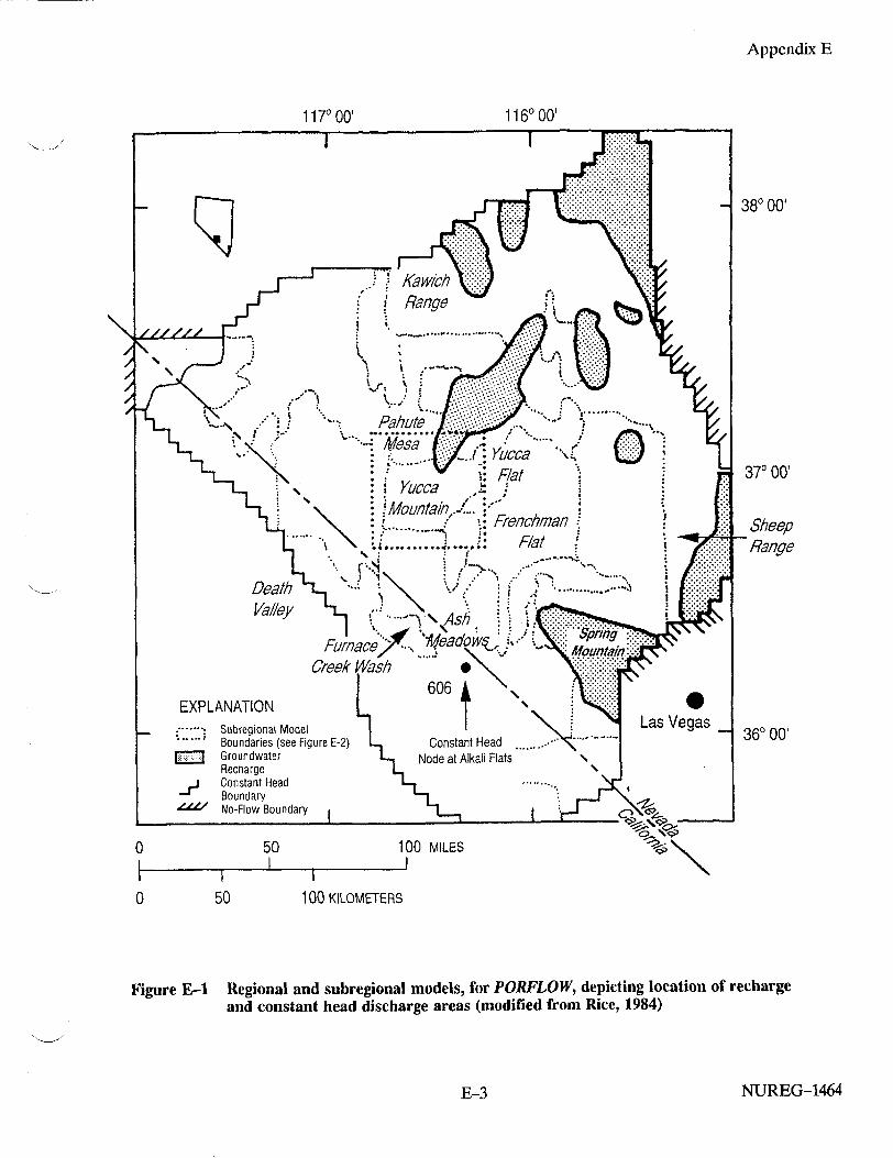
Appendix E
1170 00' 1160 00'
380 00'
370 00'
Sheep Range
360 00'
I I I 0 50 100 KILOMETERS
Regional and subregional models, for PORFLOW, depicting location of recharge and constant head discharge areas (modified from Rice, 1984)
NUREG-1464
Figure E-1
E-3

Appendix E
Discharge areas included Alkali Flats and the Furnace Creek Ranch, which were modeled as fixed head boundaries. Mathematical boundary conditions for the regional model consisted of both fixed pressures and no-flow boundaries; these boundary conditions were chosen to be consistent with the physical boundaries (Figure E-1). The regional and subregional models consisted of 13,161 and 18,225 finite difference computational cells, respectively. Each grid cell in the regional model was 2.5 kilometers on a side, encompassing an area of 6.25 square kilometers. The grid cells for the subregional model ranged from 100 meters on a side near the center to 2.5 kilometers on a side near the outer edges. The boundary conditions for this model consisted only of fixed pressures that were obtained from the simulation results of the larger regional model. The hydrological data for the simulations were obtained from the review of previously published studies (Rice, 1984; Waddell, 1982; Waddell et al., 1984; Czarnecki and Waddell, 1984; and Czarnecki, 1985).
The entire modeled region was divided into zones having one of eight possible values for the hydraulic conductivity as shown in Figure E-2 and listed in Table E-1. These hydraulic conductivities varied over several orders of magnitude, and were estimated from transmissivity data published by Rice (1984). The model contains a low permeability zone north and northeast of Yucca Mountain indicated in Figure E-2 by Zones 1 and 2 (i.e., hatched regions in the area of Yucca Mountain and Yucca Flats) for simulating the presentday high hydraulic gradient at that location. The actual cause of the steep gradient is not yet fully known.
To conduct the study, PORFLOWwas modified (Version 1.11) to incorporate the free surface (water table) in a ground-water flow model. The free-surface boundary condition and approximations (e.g., Dupuit) used in the modifications to PORFLOW are described in Bear (1988). Ahola and Sagar (1992) provide a detailed discussion of the specific modifications to PORFLOW. In essence, the model allowed 2-D flow in the horizontal plane, with the height of the water table adjusted such that the water pressure along this boundary is just equal to zero.
Table E-1 Hydraulic Conductivities for the Model
Hydraulic Conductivity
Zone Number (m/sec)
1 5.80E-08
2 6.34E-07
3 3.49E-06
4 8.69E-06
5 3.47E-05
6 L.OOE-04
7 6.OOE-04
8 3.50E-03
E-4 ANALYSES RESULTS
E-4.1 Regional Model Results
For the regional analysis, a steady-state solution to the flow system was first obtained to represent the present-day conditions under normal precipitation and ground-water recharge. Figure E-3 shows a portion of the simulated regional water table in the area of interest under assumed modern-day recharge. Yucca Mountain is indicated by the small rectangular box in this figure and represents approximately two grid nodes in the regional model (250- by 250-kilometers) because of the 2.5 kilometer grid node spacing. Thus, on the Yucca Mountain scale, the regional model is quite coarse. Based on the simulation, one can see the steep hydraulic gradient to the north and northeast of Yucca Mountain, which is comparable to results obtained in previous studies. It should be noted, however, that no calibration of this model was conducted for this study. The results are based on the use of data published from previously calibrated models. Since the results appeared consistent with previous studies and our objective was to focus more on relative changes in the water table rather than on the absolute water table elevation itself, they were deemed acceptable for use as a base case L initial state for analyzing the effects of various postulated disruptive conditions.
NUREG-1464 E-4

Appendix E
Finite Difference Grid
38000'
37o00'
36000'
Figure E-2 Regional model for PORFLOW depicting boundary conditions and various hydraulic conductivity zones (modified from Rice, 1984) (Hatched areas indicate low permeability.)
NUREG-1464
200 kn
100 km
E-5

Appendix E
180000
Pahute Mesa
170000 "
1525
160000 -10
150000 1
140000 14000 \,.5• ...--./Mountain
Area
130000
120000
825
110000
90000 100000 110000 120000 130000 140000 150000 160000
Meters
Figure E-3 Simulated hydraulic head distribution in the vicinity of Yucca Mountain, under assumed present-day conditions
NUREG-1464
CD
G)
170000
E-6
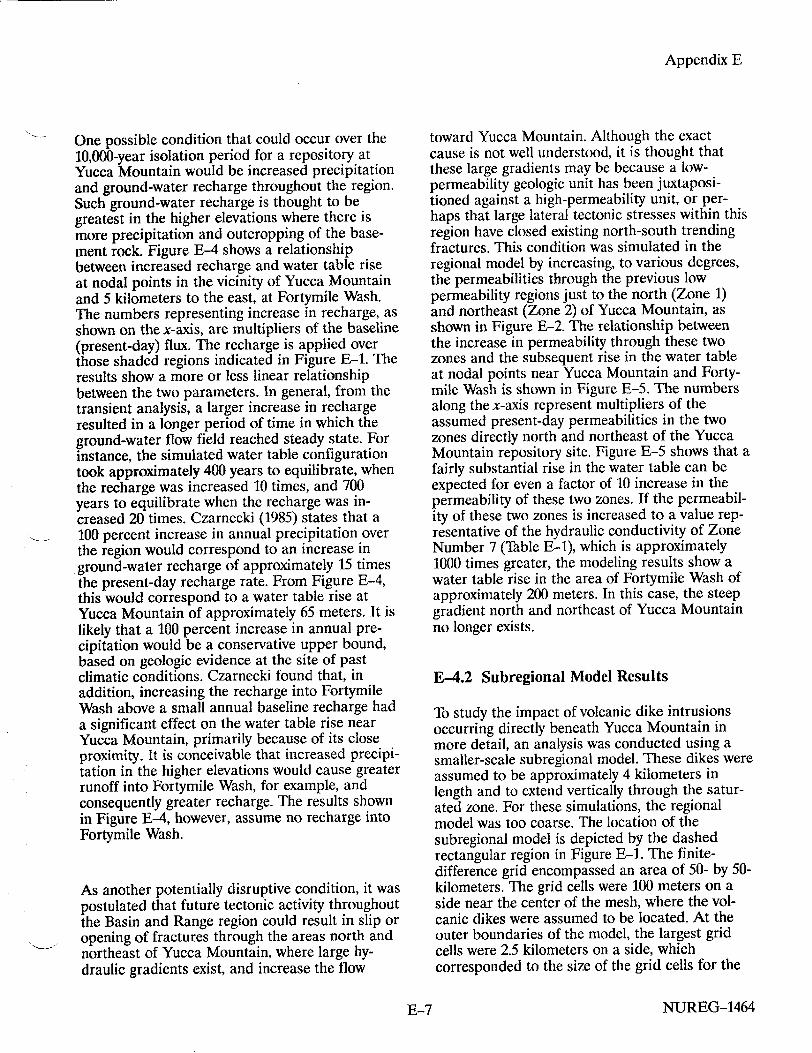
Appendix E
One possible condition that could occur over the 10,000-year isolation period for a repository at Yucca Mountain would be increased precipitation and ground-water recharge throughout the region. Such ground-water recharge is thought to be greatest in the higher elevations where there is more precipitation and outcropping of the basement rock. Figure E-4 shows a relationship between increased recharge and water table rise at nodal points in the vicinity of Yucca Mountain and 5 kilometers to the east, at Fortymile Wash. The numbers representing increase in recharge, as shown on the x-axis, are multipliers of the baseline (present-day) flux. The recharge is applied over those shaded regions indicated in Figure E-1. The results show a more or less linear relationship between the two parameters. In general, from the transient analysis, a larger increase in recharge resulted in a longer period of time in which the ground-water flow field reached steady state. For instance, the simulated water table configuration took approximately 400 years to equilibrate, when the recharge was increased 10 times, and 700 years to equilibrate when the recharge was increased 20 times. Czarnecki (1985) states that a 100 percent increase in annual precipitation over the region would correspond to an increase in ,ground-water recharge of approximately 15 times the present-day recharge rate. From Figure E-4, this would correspond to a water table rise at Yucca Mountain of approximately 65 meters. It is likely that a 100 percent increase in annual precipitation would be a conservative upper bound, based on geologic evidence at the site of past climatic conditions. Czarnecki found that, in addition, increasing the recharge into Fortymile Wash above a small annual baseline recharge had a significant effect on the water table rise near Yucca Mountain, primarily because of its close proximity. It is conceivable that increased precipitation in the higher elevations would cause greater runoff into Fortymile Wash, for example, and consequently greater recharge. The results shown in Figure E-4, however, assume no recharge into Fortymile Wash.
As another potentially disruptive condition, it was postulated that future tectonic activity throughout the Basin and Range region could result in slip or opening of fractures through the areas north and northeast of Yucca Mountain, where large hydraulic gradients exist, and increase the flow
toward Yucca Mountain. Although the exact cause is not well understood, it is thought that these large gradients may be because a lowpermeability geologic unit has been juxtapositioned against a high-permeability unit, or perhaps that large lateral tectonic stresses within this region have closed existing north-south trending fractures. This condition was simulated in the regional model by increasing, to various degrees, the permeabilities through the previous low permeability regions just to the north (Zone 1) and northeast (Zone 2) of Yucca Mountain, as shown in Figure E-2. The relationship between the increase in permeability through these two zones and the subsequent rise in the water table at nodal points near Yucca Mountain and Fortymile Wash is shown in Figure E-5. The numbers along the x-axis represent multipliers of the assumed present-day permeabilities in the two zones directly north and northeast of the Yucca Mountain repository site. Figure E-5 shows that a fairly substantial rise in the water table can be expected for even a factor of 10 increase in the permeability of these two zones. If the permeability of these two zones is increased to a value representative of the hydraulic conductivity of Zone Number 7 (Table E-1), which is approximately 1000 times greater, the modeling results show a water table rise in the area of Fortymile Wash of approximately 200 meters. In this case, the steep gradient north and northeast of Yucca Mountain no longer exists.
E-4.2 Subregional Model Results
To study the impact of volcanic dike intrusions occurring directly beneath Yucca Mountain in more detail, an analysis was conducted using a smaller-scale subregional model. These dikes were assumed to be approximately 4 kilometers in length and to extend vertically through the saturated zone. For these simulations, the regional model was too coarse. The location of the subregional model is depicted by the dashed rectangular region in Figure E-1. The finitedifference grid encompassed an area of 50- by 50kilometers. The grid cells were 100 meters on a side near the center of the mesh, where the volcanic dikes were assumed to be located. At the outer boundaries of the model, the largest grid cells were 2.5 kilometers on a side, which corresponded to the size of the grid cells for the
NUREG-1464E-7
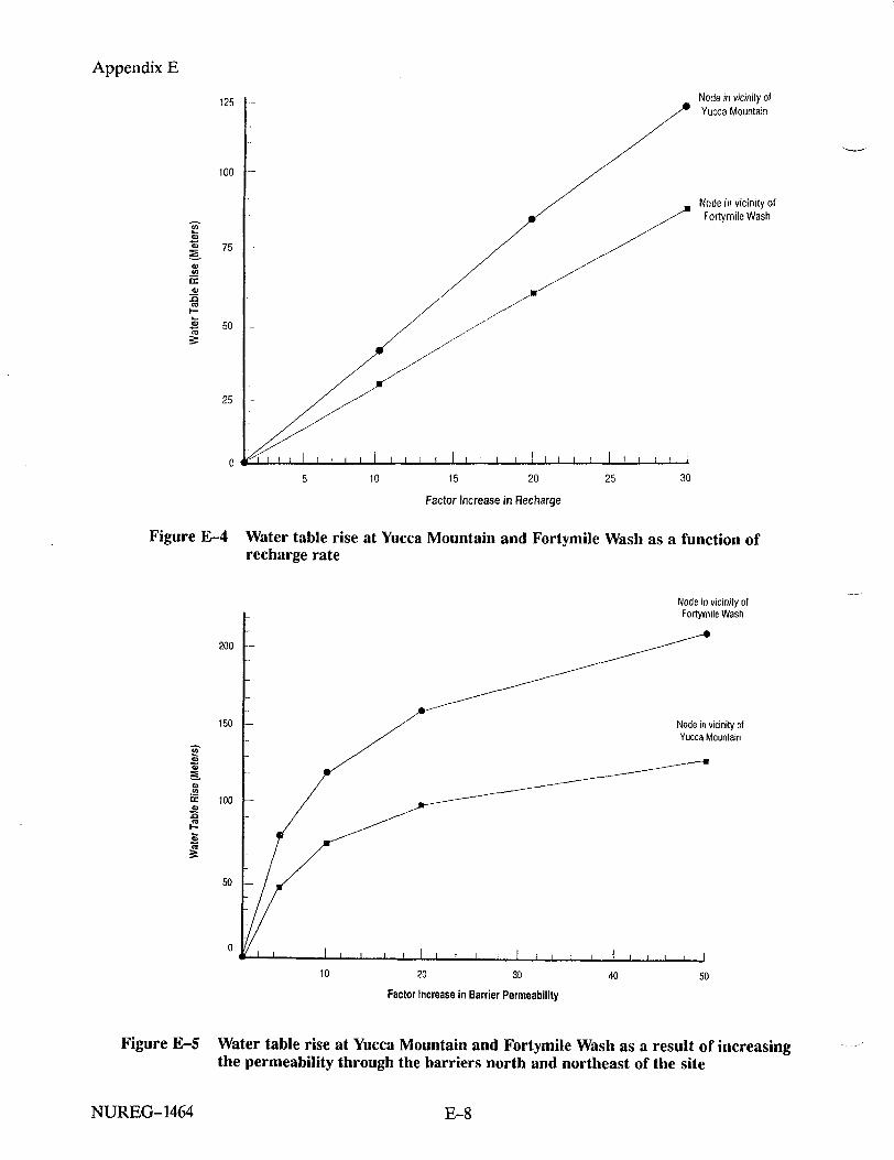
5 10 15 20 25
Factor increase in Recharge
Figure E-4
200
150
CC
C)
U) CC
0)
C) IC) C)
100
50
Water table rise at Yucca Mountain and Fortymile Wash as recharge rate
a function of
Node in vicinity of Forlymile Wash
Node in vicinity of Yucca Mountain
10 20 30 40 50
Factor Increase in Barrier Permeability
Water table rise at Yucca Mountain and Fortymile Wash as a result of increasing the permeability through the barriers north and northeast of the site
NUREG-1464
Appendix E
125
100
U) C) C)
C)
C) C)
F
C) (0
Node in vicinity of Yucca Mountain
Node in vicinity of Fortymile Wash
75
50
25
030
Figure E-5
E-8

Appendix E
regional model. The boundary conditions along all four sides of this model consisted of fixed pressures obtained from corresponding nodes in the regional model. Linear interpolation was done to assign values of pressure to those additional nodes along the boundary of the subregional model as a result of refining the mesh. These fixed boundary pressures corresponded to the baseline (or current) water table configuration from the regional model.
No attempt was made to take into account the effect the temperature of the intruding dike might have on the saturated zone. The narrow dikes essentially acted as dams within the flow field, and were assumed to extend through the water table and well above any potential water table rise. They were created by specifying a very low permeability along lines one gridpoint in thickness and 4 kilometers in length. Figure E-6 shows the velocity vectors and several streamlines (dark solid lines) depicting the ground-water flow field directly beneath Yucca Mountain, for the case of a single dike oriented N15°E, where the north direction is to the top of the plot. Based on the existing fracture and faulting pattern at Yucca Mountain, it is believed that this could be a likely orientation for a possible dike intrusion. Figure E-6 shows that to the left of the dike, the flow field can be seen to be directed toward the south. Around the lower tip of the dike, some of the flow is directed back to the north. Without the presence of the dike, the flow through this area is primarily east and southeast. The small circle in this figure indicates the location where the maximum water table rise occurred, which in this case was 79 meters. Even though the groundwater travel time through the unsaturated zone would be somewhat decreased, the travel time in the saturated zone could be substantially increased, especially for the portion of the radionuclide inventory that entered the saturated zone on the left side of the dike. Figure E-7 shows the numerical simulation results for the water table rise at the repository site for various dike orientations. The figure suggests that a dike oriented roughly north to northeast would produce the maximum water table rise for a single dike intrusion.
Figure E-8 shows the intrusion of a second dike, which is perpendicular to the one shown in Figure E-6. This case was simulated because it is believed to be not uncommon for volcanic dikes to occur in pairs at more or less perpendicular orientations. Interestingly, Figure E-8 shows the dikes create stagnant pools of water which again may increase the length of the flow path in the saturated zone to the accessible environment. The maximum water table rise for this case of two perpendicular dikes was 103.4 meters.
E-5 CONCLUSIONS
A summary of the results from both a regional and subregional ground-water flow analysis of the saturated zone surrounding Yucca Mountain, using the PORFLOW finite difference code, is presented. These results show the effects of various disruptive conditions on the water table elevations and resulting ground-water flow directions near the proposed HLW repository. The results give an indication of what conditions would have a minimal impact on the saturated zone hydrology near the site, and those that would have a major impact. A rise in water table in the area of Fortymile Wash was calculated to be greater than 200 meters, based on certain disruptive conditions simulated using the regional model. Because evapotranspiration and surface runoff were neglected, the actual rise would be less than calculated. In addition, the subregional model analysis showed a rise in the water table near the repository ranging from a few meters to as much as 103 meters, depending on the orientation of the simulated volcanic dikes.
The results presented here are meant to be preliminary and likely to change as site characterization studies at Yucca Mountain provide more accurate hydrological parameters and better information on which disruptive conditions would be more likely to occur in the future. Also, some of the assumptions in this analysis could be improved in future studies. For instance, with respect to the high water table rises predicted, the formation of new discharge areas that such rises may cause was completely neglected.
NUREG-1464E-9

Appendix E
3.25E4
3.00E4
2.75E4
2.50E4
2.25E4
***..l** 4 .4,4444 444 44 , 44 44 4 4 44 44 44
...... . ..... ......... .. .. 4 ....... ....... . ..
.. ..... ... ... 444 ,4 . 4, ,
\\\\I Z 1 I /
Si 44 4 4 444 4 ....... 4 44 44 44 44 44 44 . . . .
. . . . . .. . . . . . . . . . .I ' 4 4 4 4 4 4 4 4 44 4440 4 4 4
1\\\\. 444
t /1\../ /
"N W1.25E4 1.50E4 1.75E4 2.00E4 2.25E4
x (meters)
Figure F,-6 Impact of the intrusion of a single volcanic dike oriented NI5°E on the groundwater flow field directly below the repository (The straight line indicates the location of the dike. The 0 designates the location of the maximum water table rise (79.3 meters).)
NUREG-1464
E
2.50E4
E-10

75
50
CC
1.._
a,, 4
S25
0
00 II
"• ~Figure E--7 Maximum water table rise at potential repository site as a function of dik
4-a
125
•e orientation
(

Appendix E
3.25E4
3.00E4
E 2.75E4
2.50E4
2.25E41.25E4
..... ................ .. ...... ......... . .... .. .. . .. . ... .....
I~~~ ~ "."• .... ..., ...... \ \.I. . . . . ... .I . . . .. .'
,, ~ .. . . .. . .. . , , ,, , , ..,
L, , --. - --\\'\ n.... \\V£• \\NN , T
1.50E4 1.75E4 2.00E4 2.25E4 2.50E4
x (meters)
Figure E-8
NUREG-1464
Impact of the intrusion of multiple volcanic dikes on the ground-water flow field directly below the repository. (The straight lines indicate the location of the dikes. The 0 designates the location of the maximum water table rise (103.4 meters).)
E-12

Appendix E
E-6 REFERENCES
Ahola, M.P. and B. Sagar, "Regional Groundwater Modeling of the Saturated Zone in the Vicinity of Yucca Mountain, Nevada," U.S. Nuclear Regulatory Commission, NUREG/CR-5890, October 1992. [Prepared by the Center for Nuclear Waste Regulatory Analyses.]
Bear, J., Dynamics of Fluids in Porous Media, New York, Dover Publications, Inc., 1988.
Czarnecki, J.B. and R.J. Waddell, "Finite-Element Simulation of Groundwater Flow in the Vicinity of Yucca Mountain, Nevada-California, "U.S. Geological Survey, Water Resources Investigations Report, WRI-84-4349, 1984.
Czarnecki, J.B., "Simulated Effects of Increased Recharge on the Groundwater Flow System of Yucca Mountain and Vicinity, NevadaCalifornia," U.S. Geological Survey, WaterResources Investigations Report, WRI-84-4344, 1985.
Rice, WA., "Preliminary Two-Dimensional Regional Hydrologic Model of Nevada Test Site and Vicinity," Sandia National Laboratories, SAND83-7466, August 1984. [Prepared for the U.S. Department of Energy.]
Runchal, A.K. and B. Sagar, "PORFLOW: A Mathematical Model for Fluid Flow, Heat, and Mass Transport in Variably Saturated Geologic Media-Users Manual (Version 1.0), Richland, Washington, Westinghouse Hanford Company, WHC-EP-0041, July 1989.
Sagar, B. and A.K. Runchal, "PORFLOW: A Mathematical Model for Fluid Flow, Heat, and Mass Transport in Variably Saturated Geologic Media-Theory and Numerical Methods (Version 1.0)," Richland, Washington, Westinghouse Hanford Company, WHC-EP-0042, March 1990.
U.S. Department of Energy, "Site Characterization Plan, Yucca Mountain Site, Nevada Research and Development Area, Nevada," Nevada Operations Office/Yucca Mountain Project Office, Nevada, DOE/RW-0199, 9 vols., December 1988.
Waddell, R.K., "Two-Dimensional, Steady-State Model of Ground Water Flow, Nevada Test Site and Vicinity, Nevada-California," U.S. Geological Survey Water-Resources Investigations Report, WRI-82-4085, 1982.
Waddell, R.K., J.H. Robison, and R.K. Blankennagel, "Hydrology of Yucca Mountain and Vicinity, Nevada-California: Investigative Results Through Mid1983," U.S. Geological Survey Water Resources Investigation Report, WRI-84-4267, 1984.
NUREG-1464E-13

APPENDIX F EFFECTS OF STRATIFICATION, DIP OF STRATA,
AND SUB-VERTICAL FAULTS
F-1 INTRODUCTION
This section presents results of unsaturated flow simulations undertaken as an auxiliary analysis for the Iterative Performance Assessment (IPA) Phase 2 project, one of the approaches adopted by the U.S. Nuclear Regulatory Commission (NRC) staff to develop its license application review capabilities. The effects of common geological features on flow in a two-dimensional (2-D) domain, such as inclined stratification and vertical or near-vertical fault zones intersecting the strata, are of importance. In this work, numerical analysis is performed for a deep (approximately 530 meters) hard rock system. The BIGFLOW numerical code (Bagtzoglou et al., 1992) is used in these simulations. Some of the data (i.e., the depth to water table, the number of primary geologic strata, their dip angle, and the existence of a fault zone) for the analysis were taken from the Yucca Mountain project reports (Scott and Bonk, 1984), but were adjusted to enhance the effects under study. In particular, extreme net infiltration rates (up to 50 millimeters/year) and hydraulic properties similar to the Calico Hills nonwelded, vitric (Chnv) unit were considered. Therefore, conclusions regarding the suitability of Yucca Mountain for the proposed geologic repository for high-level radioactive waste are not directly derivable from this analysis. Recognizing that there are no simple, natural initial-boundary conditions that can be used for the more complex problems, a method of successive approximation is implemented. This method uses solutions of auxiliary flow problems to set up pressure boundary conditions for the more complex problems. This is necessary because, in practice, no natural boundaries exist (or are adequately defined), especially in the lateral directions. The investigation is limited to threedimensional (3-D) simulations in a vertical, thin slice, cross-section, with dipping strata intersected by a subvertical fault zone. The simulations are performed in a transient mode to study the manner in which the solutions of the flow equation approach steady state. A "wet," in terms of perceived net infiltration rates, hydroclimatic
condition corresponding to a net annual infiltration rate of 50 millimeters/year is modeled. A hypothetical test problem is developed to study the effects of bedding, presence of a subvertical fault, and inclination of the beds.
The BIGFLOW simulation code accommodates 3-D transient or steady flow in saturated, or partially saturated, porous media with heterogeneous or spatially random hydrodynamic coefficients. For partially saturated flow, a mixed variable formulation of Richards' equation is used. That is:
aO (h,x) = V IK(h,x) (Vh + g)] at (F-1)
where h is pressure head (meters), 0 is volumetric water content (cubic meters/cubic meters), K is hydraulic conductivity (meters/second), and g is the body force unit vector aligned with, and opposed to, the acceleration of gravity. The differential equations are discretized by an implicit finite difference scheme, two-point backward Euler in time, and seven-point centered in space. The spatial mesh is a regular rectangular lattice. The time step is generally variable and self-adjusted. The computational domain is a 3-D parallelepiped, whose coordinate system may be inclined at arbitrary angles with respect to the natural, horizontal-vertical coordinate system.
F-2 DESCRIPTION OF ANALYSES
The hydrogeologic properties in the unsaturated zone of Yucca Mountain, Nevada, were considered in order to represent, to some degree, the general features of the site in the simulations. Yucca Mountain consists of a series of Northtrending fault-block ridges composed of strata of volcanic ash tuffs that generally have a regional dip of 50 to 70 to the East (Scott and Bonk, 1984). The proposed repository area is also bounded by steeply dipping faults or by fault zones, and is transected by a few normal faults. Therefore, it is important to study the effects of stratification,
NUREG-1464F-1

Appendix F
regional dipping, and fault zones on unsaturated water flow.
In the simulations presented herein, the computational domain is assumed to consist of five strata with approximately equal thicknesses spanning a total depth of 530 meters at which depth the water table is assumed to be located. The computational domain used in these simulations is based on a 3-D Cartesian grid system. The axes of this system are aligned with East-West (x-axis), North-South (y-axis), and vertical (z-axis). The dimensions of the computational domain are 1230 meters, 80 meters, and 530 meters in the x-, y-, and z-directions, respectively. The domain is discretized into 29 by 5 by 54 nodes, comprising a total of 7830 nodes (Figure F-i).
The functional forms of pressure-dependent hydraulic conductivity and water content used
Y
herein are the exponential Gardner model for K(h) and the van Genuchten model for O(h). The exponential conductivity model is:
K(h) = K, exp [a(h-hb)] , if h < h,
(F-2)
K(h) = K,, if h > hb
where K, is the saturated hydraulic conductivity, a is a characteristic inverse length scale or capillary diffusivity (Ababou, 1991), h is the pressure, and ib is the air-entry pressure. The van Genuchten model for the retention curve is:
o(h) = o, + (0, - 0) [1 + (-/h)nl-m
where O, and 0, are the saturated and residual moisture contents, respectively, #3 is a characteristic inverse length (similar to a in Equation
Fault Zone
X
Figure F-I
NUREG-1464
Computational grid
(F-3)
F-2
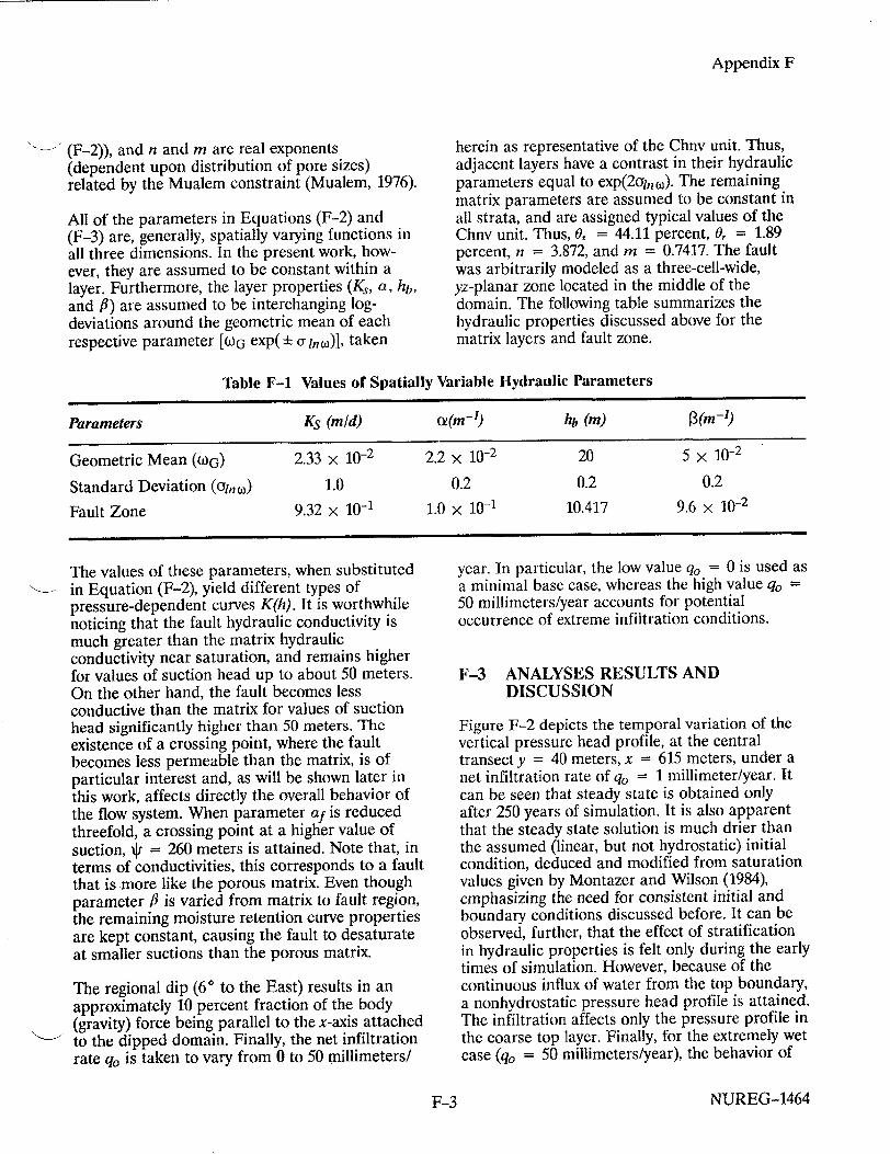
Appendix F
(F-2)), and n and m are real exponents (dependent upon distribution of pore sizes) related by the Mualem constraint (Mualem, 1976).
All of the parameters in Equations (F-2) and (F-3) are, generally, spatially varying functions in all three dimensions. In the present work, however, they are assumed to be constant within a layer. Furthermore, the layer properties (Ks, a, hb, and fP) are assumed to be interchanging logdeviations around the geometric mean of each respective parameter [w)G exp( ± cr1, w)], taken
herein as representative of the Chnv unit. Thus, adjacent layers have a contrast in their hydraulic parameters equal to exp(2oi,1•). The remaining matrix parameters are assumed to be constant in all strata, and are assigned typical values of the Chnv unit. Thus, 0. = 44.11 percent, 0 = 1.89 percent, n = 3.872, and m = 0.7417. The fault was arbitrarily modeled as a three-cell-wide, yz-planar zone located in the middle of the domain. The following table summarizes the hydraulic properties discussed above for the matrix layers and fault zone.
Table F-1 Values of Spatially Variable Hydraulic Parameters
Parameters KS (mid) oe(m-) hb (m) 1(m 1)
Geometric Mean (WoG) 2.33 x 10⁻² 2.2 x 10⁻² 20 5 x 10⁻²
Standard Deviation (on o) 1.0 0.2 0.2 0.2
Fault Zone 9.32 x 10⁻¹ 1.0 x 10⁻¹ 10.417 9.6 x 10⁻²
The values of these parameters, when substituted in Equation (F-2), yield different types of pressure-dependent curves K(h). It is worthwhile noticing that the fault hydraulic conductivity is much greater than the matrix hydraulic conductivity near saturation, and remains higher for values of suction head up to about 50 meters. On the other hand, the fault becomes less conductive than the matrix for values of suction head significantly higher than 50 meters. The existence of a crossing point, where the fault becomes less permeable than the matrix, is of particular interest and, as will be shown later in this work, affects directly the overall behavior of the flow system. When parameter af is reduced threefold, a crossing point at a higher value of suction, * = 260 meters is attained. Note that, in terms of conductivities, this corresponds to a fault that is more like the porous matrix. Even though parameter fl is varied from matrix to fault region, the remaining moisture retention curve properties are kept constant, causing the fault to desaturate at smaller suctions than the porous matrix.
The regional dip (60 to the East) results in an approximately 10 percent fraction of the body (gravity) force being parallel to the x-axis attached "to the dipped domain. Finally, the net infiltration rate q0 is taken to vary from 0 to 50 millimeters/
year. In particular, the low value q, = 0 is used as a minimal base case, whereas the high value q0 50 millimeters/year accounts for potential occurrence of extreme infiltration conditions.
F-3 ANALYSES RESULTS AND DISCUSSION
Figure F-2 depicts the temporal variation of the vertical pressure head profile, at the central transect y = 40 meters, x = 615 meters, under a net infiltration rate of q0 = 1 millimeter/year. It can be seen that steady state is obtained only after 250 years of simulation. It is also apparent that the steady state solution is much drier than the assumed (linear, but not hydrostatic) initial condition, deduced and modified from saturation values given by Montazer and Wilson (1984), emphasizing the need for consistent initial and boundary conditions discussed before. It can be observed, further, that the effect of stratification in hydraulic properties is felt only during the early times of simulation. However, because of the continuous influx of water from the top boundary, a nonhydrostatic pressure head profile is attained. The infiltration affects only the pressure profile in the coarse top layer. Finally, for the extremely wet case (qo = 50 millimeters/year), the behavior of
NUREG-1464F-3
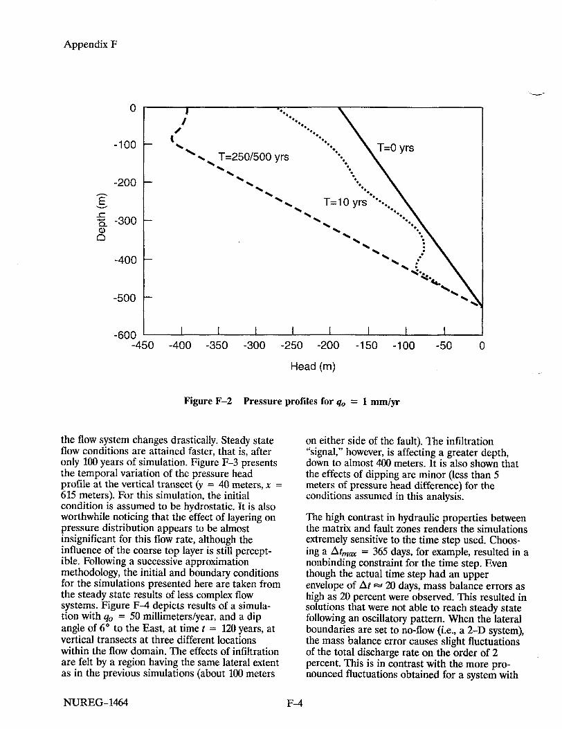
Appendix F
0
-100
-200
-300
-400
-500
-600 -450 -400 -350 -300 -250 -200 -150 -100 -50 0
Head (m)
Figure F-2 Pressure
the flow system changes drastically. Steady state flow conditions are attained faster, that is, after only 100 years of simulation. Figure F-3 presents the temporal variation of the pressure head profile at the vertical transect (y = 40 meters, x = 615 meters). For this simulation, the initial condition is assumed to be hydrostatic. It is also worthwhile noticing that the effect of layering on pressure distribution appears to be almost insignificant for this flow rate, although the influence of the coarse top layer is still perceptible. Following a successive approximation methodology, the initial and boundary conditions for the simulations presented here are taken from the steady state results of less complex flow systems. Figure F-4 depicts results of a simulation with q = 50 millimeters/year, and a dip angle of 60 to the East, at time t = 120 years, at vertical transects at three different locations within the flow domain. The effects of infiltration are felt by a region having the same lateral extent as in the previous simulations (about 100 meters
profiles for q, = 1 mm/yr
on either side of the fault). The infiltration "signal," however, is affecting a greater depth, down to almost 400 meters. It is also shown that the effects of dipping are minor (less than 5 meters of pressure head difference) for the conditions assumed in this analysis.
The high contrast in hydraulic properties between the matrix and fault zones renders the simulations extremely sensitive to the time step used. Choosing a Atm,, = 365 days, for example, resulted in a nonbinding constraint for the time step. Even though the actual time step had an upper envelope of At ,t 20 days, mass balance errors as high as 20 percent were observed. This resulted in solutions that were not able to reach steady state following an oscillatory pattern. When the lateral boundaries are set to no-flow (i.e., a 2-D system), the mass balance error causes slight fluctuations of the total discharge rate on the order of 2 percent. This is in contrast with the more pronounced fluctuations obtained for a system with
NUREG-1464
E
F-4

Appendix F
0
-100
-200
t-• -300
-400
-500
-600 ' -600 -500 -400 -300 -200 -100
Head (m)
Figure F-3 Pressure profiles for qo, = 50 mm/yr
0-200 -150 -100 -50
Head (m)
Figure F-4 Pressure profiles for qo = 50 mm/yr and a dip angle of 60
NUREG-1464
0
0
--, -200 E
0
o-400
-600 1 -250
F-5

Appendix F
the fault cutting Dirichlet boundaries. It was found that in order to obtain a well-behaved numerical solution, with clearly stable convergence to steady state, the time step had to be drastically reduced. When the maximum time step was decreased to Atma, = 10 days, the mass balance plots indicated a complete elimination of large mass balance errors (except for early transients). The conclusion in this case is that, although the discrete-time system was unstable, the continuous time system corresponding to a vanishingly small time step (At -+ 0) is, in fact, stable and leads to a unique steady state solution as t -4 oo. While this phenomenon results from the discreetness (in time) of the numerical flow problem, it indicates a peculiar phenomenon related with the 3-D configuration of the faulted domain and with the direct connection between fault and permeable boundaries.
The steady state flow pattern in each case is best represented by 2-D vector plots of the unsaturated water velocity (or flux), and particle tracks depicting the locations of particles released in the steady flow system at selected points. These 2-D vector and particle tracks are shown in Figures F-5a and F-5b for the higher and milder property contrast case, respectively. Inspection of these figures clearly shows a significant effect of the contrast between slopes of the matrix/fault unsaturated conductivities. When the fault's conductivity slope is comparatively much larger than that of the matrix (am = 0.022 meters- 1, af = 0.10 meters-1 ), higher fluxes were observed in the matrix. This results in a front that lags within the fault zone. Figure F-5(a) shows this effect for two lines of particles released at elevations 500 meters and 300 meters, respectively, and tracked for 1000 years. In this case, the maximum distance traveled in 1,000 years is approximately 67 meters. When the contrast is milder (am, = 0.022 meters- 1, af = 0.035 meters-1 ), the opposite behavior is observed. The fluxes within the fault zone are greater, but they point towards the matrix (Figure F-5(b)). This creates a frontal shape that continuously expands outward from the fault zone. In this case, the maximum distance traveled in 1000 years is 165 meters and more than 200 meters, for the two release planes, respectively. This important difference in behavior is because of the different values of the crossing- point suction in the two cases. Recall that the contrast between matrix and fault moisture retention curves was not changed. As a
consequence, the steady state moisture patterns above the water table are almost identical for the two contrast cases studied. What is important to keep in mind is that the travel time of particles is sensitive to the unsaturated conductivity slope, even when the moisture retention curve is held constant.
F-4 CONCLUSIONS
A hypothetical test problem was developed in order to study the effect of bedding on flow, the presence of a subvertical fault zone, and the effect of inclination of the beds. A number of auxiliary tests were also conducted, using variations on these hypothetical data. There are some similarities between this hypothetical problem and the Yucca Mountain stratigraphy, but since all site properties are not used, these simulations are not representative of the Yucca Mountain flow conditions.
Recognizing that there may not be natural initialboundary conditions that can be used for the more complex problems, a method of successive approximation was implemented. This method uses solutions of auxiliary flow problems to set up pressure conditions for more complex problems. An oscillatory flow regime was observed at large times, that is, after initial transients died out. This was shown to be an effect of the discrete-time nature of the equations being solved, and was eliminated by using extremely small time steps (At --* 0). The techniques used to identify these effects relied on detailed plots of global mass balance in terms of instantaneous net discharge rate and instantaneous rate of change of total mass. Large At yielded oscillations for both 2-D and 3-D flow systems, but seemed more consequential in 3-D (fault-cutting pressure boundaries).
Based on the parameters used, and the simulations performed in this study, the following conclusions can be reached:
"* The effects of stratification are important only for low net infiltration rates and during the early parts of transient simulations.
"* A dip angle of 6' to the East has a minimal effect on the pressure head distributions (approximately 2 percent of the maximum pressure head difference).
NUREG-1464 F-6
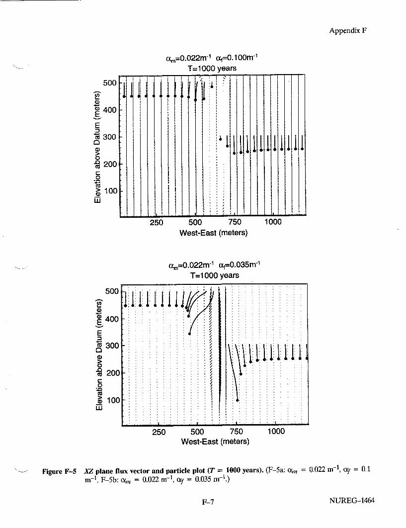
Appendix F
am=0.022m-1 a1=0.100m-1 T=1000 years
I I IIIIIII1L
. . ,I I , I! 21 . .d -. , -" . ,, . .. . . .
250 500 750 1000
West-East (meters)
am=0.022m-1 af=0.0 3 5 m-' T=I 000 years
S .. . . . . . . . . . .
S. . .. . . . . .
S.. . . . . . . . / . . . . . . . . S.. .. . . . . . . . . . .. . . .
500 750 1000West-East (meters)
Figure F-5 XZ plane flux vector and particle plot (T = 1000 years). (F-5a: Oa, = 0.022 m-1, of = 0.1 m-1. F-5b: otm = 0.022 m- 1, of = 0.035 m- 1.)
NUREG-1464
I500
( 400 E
E
"E" 300 0 CD
"- 200
0
>100 LU
500
0)
400 E E
300
. 200 0
S100 ED
250
F-7
I

Appendix F
* The flow behavior (ground-water fluxes and travel times) of a system consisting of highly contrasted matrix and vertical fault properties is greatly influenced by the ratio of the slopes of the matrix and fault unsaturated hydraulic conductivity curves.
F-5 REFERENCES
Ababou R., 'Approaches to Large Scale Unsaturated Flow on Heterogeneous, Stratified, and Fractured Geologic Media," U.S. Nuclear Regulatory Commission, NUREG/CR-5743, August 1991. [Prepared by the Center for Nuclear Waste Regulatory Analyses.]
Bagtzoglou, A.C., R. Ababou, and A. Nedungadi, "BIGFLOW: A Multi-Dimensional Code for Flow in Heterogeneous and Variably Saturated Geologic Media (Theory and User's Manual-Version
1.0)," Center for Nuclear Waste Regulatory Analyses, CNWRA92-026, December 1992. [Prepared for the U.S. Nuclear Regulatory Commission.]
Montazer, P. and WE. Wilson, "Conceptual Hydrologic Model of Flow in the Unsaturated Zone, Yucca Mountain, Nevada," U.S. Geological Survey, Water Resources Investigation Report, WRI-84-4345, 1984.
Mualem, Y., 'A Catalogue of the Hydraulic Properties of Unsaturated Soils," Haifa, Israel, Technion Institute of Technology, Hydrodynamics and Hydraulic Laboratory, Research Project No. 442, 1976.
Scott, R.B. and J. Bonk, "Preliminary Geologic Map of Yucca Mountain with Geologic Sections, Nye County, Nevada," U.S. Geological Survey, Open-File Report 84-494, 1984.
NUREG-1464 F-8
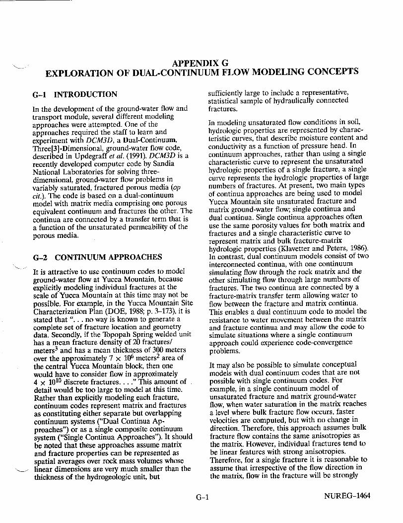
APPENDIX G EXPLORATION OF DUAL-CONTINUUM FLOW MODELING CONCEPTS
G-1 INTRODUCTION
In the development of the ground-water flow and transport module, several different modeling approaches were attempted. One of the approaches required the staff to learn and experiment with DCM3D, a Dual-Continuum, Three[3]-Dimensional, ground-water flow code, described in Updegraff et al. (1991). DCM3D is a recently developed computer code by Sandia National Laboratories for solving threedimensional, ground-water flow problems in variably saturated, fractured porous media (op cit.). The code is based on a dual-continuum model with matrix media comprising one porous equivalent continuum and fractures the other. The continua are connected by a transfer term that is a function of the unsaturated permeability of the porous media.
G-2 CONTINUUM APPROACHES
It is attractive to use continuum codes to model ground-water flow at Yucca Mountain, because explicitly modeling individual fractures at the scale of Yucca Mountain at this time may not be possible. For example, in the Yucca Mountain Site Characterization Plan (DOE, 1988; p. 3-173), it is stated that ".. . no way is known to generate a complete set of fracture location and geometry data. Secondly, if the Topopah Spring welded unit has a mean fracture density of 20 fractures/ meters 3 and has a mean thickness of 300 meters over the approximately 7 x 10⁶ meters2 area of the central Yucca Mountain block, then one would have to consider flow in approximately 4 x 10¹⁰ discrete fractures... ." This amount of detail would be too large to model at this time. Rather than explicitly modeling each fracture, continuum codes represent matrix and fractures as constituting either separate but overlapping continuum systems ("Dual Continua Approaches") or as a single composite continuum system ("Single Continua Approaches"). It should be noted that these approaches assume matrix and fracture properties can be represented as spatial averages over rock mass volumes whose linear dimensions are very much smaller than the thickness of the hydrogeologic unit, but
sufficiently large to include a representative, statistical sample of hydraulically connected fractures.
In modeling unsaturated flow conditions in soil, hydrologic properties are represented by characteristic curves, that describe moisture content and conductivity as a function of pressure head. In continuum approaches, rather than using a single characteristic curve to represent the unsaturated hydrologic properties of a single fracture, a single curve represents the hydrologic properties of large numbers of fractures. At present, two main types of continua approaches are being used to model Yucca Mountain site unsaturated fracture and matrix ground-water flow; single continua and dual continua. Single continua approaches often use the same porosity values for both matrix and fractures and a single characteristic curve to represent matrix and bulk fracture-matrix hydrologic properties (Klavetter and Peters, 1986). In contrast, dual continuum models consist of two interconnected continua, with one continuum simulating flow through the rock matrix and the other simulating flow through large numbers of fractures. The two continua are connected by a fracture-matrix transfer term allowing water to flow between the fracture and matrix continua. This enables a dual continuum code to model the resistance to water movement between the matrix and fracture continua and may allow the code to simulate situations where a single continuum approach could experience code-convergence problems.
It may also be possible to simulate conceptual models with dual continuum codes that are not possible with single continuum codes. For example, in a single continuum model of unsaturated fracture and matrix ground-water flow, when water saturation in the matrix reaches a level where bulk fracture flow occurs, faster velocities are computed, but with no change in direction. Therefore, this approach assumes bulk fracture flow contains the same anisotropies as the matrix. However, individual fractures tend to be linear features with strong anisotropies. Therefore, for a single fracture it is reasonable to assume that irrespective of the flow direction in the matrix, flow in the fracture will be strongly
NUREG-1464G-1
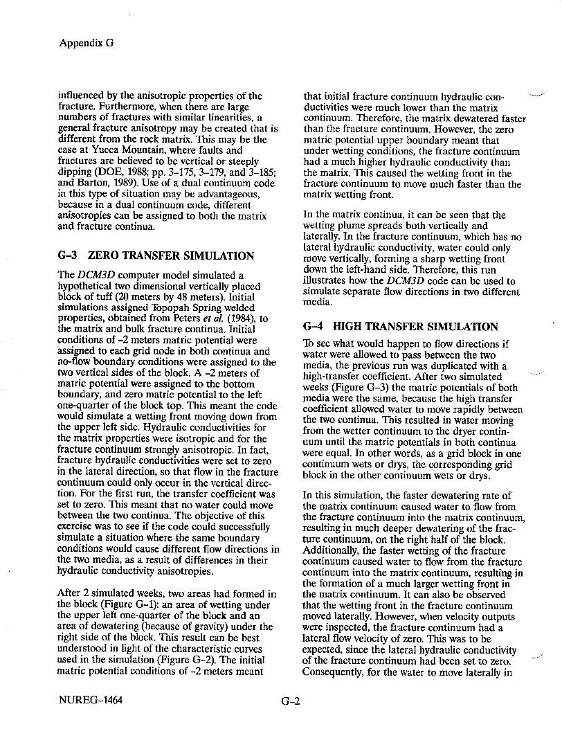
Appendix G
influenced by the anisotropic properties of the fracture. Furthermore, when there are large numbers of fractures with similar linearities, a general fracture anisotropy may be created that is different from the rock matrix. This may be the case at Yucca Mountain, where faults and fractures are believed to be vertical or steeply dipping (DOE, 1988; pp. 3-175, 3-179, and 3-185; and Barton, 1989). Use of a dual continuum code in this type of situation may be advantageous, because in a dual continuum code, different anisotropies can be assigned to both the matrix and fracture continua.
G-3 ZERO TRANSFER SIMULATION
The DCM3D computer model simulated a hypothetical two dimensional vertically placed block of tuff (20 meters by 48 meters). Initial simulations assigned Topopah Spring welded properties, obtained from Peters et a[. (1984), to the matrix and bulk fracture continua. Initial conditions of -2 meters matric potential were assigned to each grid node in both continua and no-flow boundary conditions were assigned to the two vertical sides of the block. A -2 meters of matric potential were assigned to the bottom boundary, and zero matric potential to the left one-quarter of the block top. This meant the code would simulate a wetting front moving down from the upper left side. Hydraulic conductivities for the matrix properties were isotropic and for the fracture continuum strongly anisotropic. In fact, fracture hydraulic conductivities were set to zero in the lateral direction, so that flow in the fracture continuum could only occur in the vertical direction. For the first run, the transfer coefficient was set to zero. This meant that no water could move between the two continua. The objective of this exercise was to see if the code could successfully simulate a situation where the same boundary conditions would cause different flow directions in the two media, as a result of differences in their hydraulic conductivity anisotropies.
After 2 simulated weeks, two areas had formed in the block (Figure G-1): an area of wetting under the upper left one-quarter of the block and an area of dewatering (because of gravity) under the right side of the block. This result can be best understood in light of the characteristic curves used in the simulation (Figure G-2). The initial matric potential conditions of -2 meters meant
that initial fracture continuum hydraulic conductivities were much lower than the matrix continuum. Therefore, the matrix dewatered faster than the fracture continuum. However, the zero matric potential upper boundary meant that under wetting conditions, the fracture continuum had a much higher hydraulic conductivity than the matrix. This caused the wetting front in the fracture continuum to move much faster than the matrix wetting front.
In the matrix continua, it can be seen that the wetting plume spreads both vertically and laterally. In the fracture continuum, which has no lateral hydraulic conductivity, water could only move vertically, forming a sharp wetting front down the left-hand side. Therefore, this run illustrates how the DCM3D code can be used to simulate separate flow directions in two different media.
G-4 HIGH TRANSFER SIMULATION
To see what would happen to flow directions if water were allowed to pass between the two media, the previous run was duplicated with a high-transfer coefficient. After two simulated weeks (Figure G-3) the matric potentials of both media were the same, because the high transfer coefficient allowed water to move rapidly between the two continua. This resulted in water moving from the wetter continuum to the dryer continuum until the matric potentials in both continua were equal. In other words, as a grid block in one continuum wets or drys, the corresponding grid block in the other continuum wets or drys.
In this simulation, the faster dewatering rate of the matrix continuum caused water to flow from the fracture continuum into the matrix continuum, resulting in much deeper dewatering of the fracture continuum, on the right half of the block. Additionally, the faster wetting of the fracture continuum caused water to flow from the fracture continuum into the matrix continuum, resulting in the formation of a much larger wetting front in the matrix continuum. It can also be observed that the wetting front in the fracture continuum moved laterally. However, when velocity outputs were inspected, the fracture continuum had a lateral flow velocity of zero. This was to be expected, since the lateral hydraulic conductivity of the fracture continuum had been set to zero. Consequently, for the water to move laterally in
N-UREG-1464 G-2

Appendix G
Fractures
Wetting Dewatering
47 45 43
41 39
37
35 33 31
29
27
25 23 21
19 17 15
13 11
9
7
5 3 1
1 3 5 7 9 11 13 1517 19 Meters
47 45 43
41 39
37
35 33 31
29
27
25 23 21 19
17 15
13 11
9
7
5 3 1
Wetting Dewatering
1 3 5 7 9 11 13 15 17 19 Meters
Contour plot of matric potentials for hypothetical block of Topopah Spring tuff matrix and fracture continua after simulating two weeks of flow (There is no flow between the two continua.)
NUREG-1464
Matrix
(I) L.. a,
4-' a,
Uf) W
Figure G-1
G-3

Appendix G
2
4
"1
0 C)
104
103 102
10 1
10-1 10-2
10-3 10-4
10-5
10-6
10-7
10-8
10-9 10-10
10-11 10-12
10-13
10-14
10-15
10-16
10-17
10-2 10-1 1 10 102
Pressure Head (-M)
Figure G-2 Topopah Spring welded unit fracture and matrix properties
NUREG-1464
103
G-4
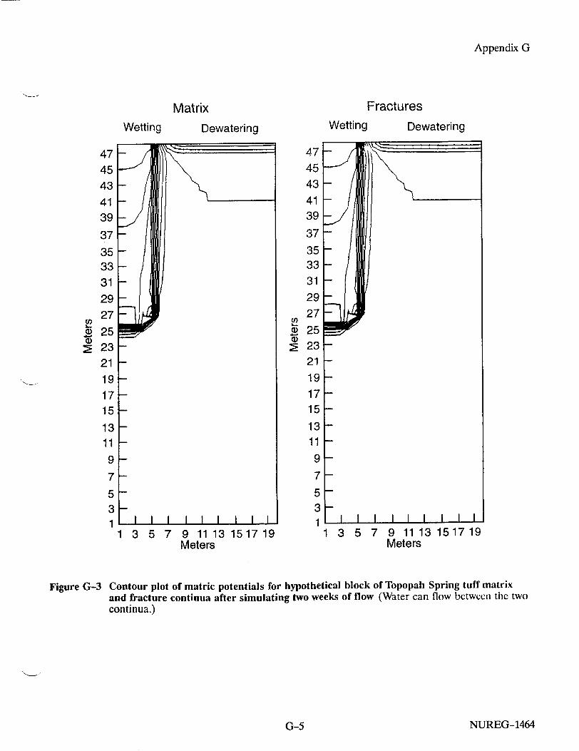
Appendix G
Fractures
Dewatering Wetting Dewatering
1357
47 45 43
41 39
37
35 33
31
29
27
25 23 21
19
17 15
13 11
9
7
5 3 1
9 11 13 15 17 19 Meters
47
45 43
41 39
37
35 33
31
29
27
25 23 21
19
17 15
13 11
9
7
5 3 1
1 3 5 7 9 11 13 15 17 19 Meters
Contour plot of matric potentials for hypothetical block of Topopah Spring tuff matrix and fracture continua after simulating two weeks of flow (Water can flow between tile two continua.)
NUREG-1464
MatrixWetting
(U L.. 0) 4ci)
CD
Figure G-3
G-5

Appendix G
the fracture continuum, it first had to move into the matrix continuum, move laterally in the matrix continuum, and then move back into the fracture continuum. In nature, this would be analogous to flowing fractures wetting up the matrix, which, in turn, causes other fractures to flow. Therefore, an interpretation of model matric potentials, water contents, and velocities, which ignores water movement between the two continua, may be misleading about the rate and direction of fluid flow.
G-5 SIMULATION COMPARING SINGLE AND DUAL CONTINUUM APPROACHES
To further compare the single and dual continuum approaches, the DCM3D input was modified to make it simulate a single continuum approach. In a single continuum code, the combined matrix and fracture flow properties are assumed to have the same porosities and the same hydraulic conductivity anisotropies.
It was decided to make DCM3D mimic a single continuum code by assigning isotropic hydraulic conductivities to the fracture continuum, and to repeat the high transfer coefficient run. It was a little less clear what porosity values should be input. If a single porosity value were used for both the matrix and fracture continua, the simulation would contain a much higher total pore space than a single continuum approach would use. It was therefore decided to leave the porosity values the same as the previous high-transfer coefficient run. This meant that the matrix continuum had a porosity of 0.11 and that the fracture continuum, had a porosity of 1.8 x 10-. This was believed to be a reasonable compromise, since, in a single continuum approach, fracture flow is simulated when the pore space is nearly filled. The output from the previous dual continuum high-transfer run and the simulated single continuum run is compared in Figure G-4. This comparison shows that the lack of lateral fracture conductivity in the
dual continuum simulation caused the wetting front to travel deeper, with less lateral spreading than the single continuum simulation.
G-5 CONCLUSIONS
These simulations demonstrate that the dual continuum code DCM3D can model flow in two continua with different anisotropies and that, depending on the problem to be modeled, it may produce significantly different answers than a single continuum code.
G-6 REFERENCES
Barton, C., W. Page, and T Morgan, "Fractures in Outcrops in the Vicinity of Drill Hole USW G-4, Yucca Mountain, Nevada, Data Analysis and Compilation," U.S. Geological Survey, Open File Report 89-92, 1989.
Klavetter, E.A. and R.P. Peters, "Fluid Flow in a Fractured Rock Mass," Albuquerque, New Mexico, Sandia National Laboratories, SAND85-0855, March 1986.
Peters, R. R., et al., "Fracture and Matrix Hydrologic Characteristics of Tuffaceous Materials from Yucca Mountain, Nye County, Nevada," Albuquerque, New Mexico, Sandia National Laboratories, SAND84-1471, December 1984.
Updegraff, C.D., C.E. Lee, and D.P. Gallegos, "DCM3D: A Dual-Continuum, ThreeDimensional, Ground-Water Flow Code for Unsaturated, Fractured, Porous Media," U.S. Nuclear Regulatory Commission, NUREG/CR5536, February 1991. [Prepared by the Sandia National Laboratories.]
U.S. Department of Energy, "Site Characterization Plan Overview, Yucca Mountain Site, Nevada Research and Development Area, Nevada," Office of Civilian Radioactive Waste Management, DOE/RW-0198, 9 vols., December 1988.
NUREG-1464 G-6
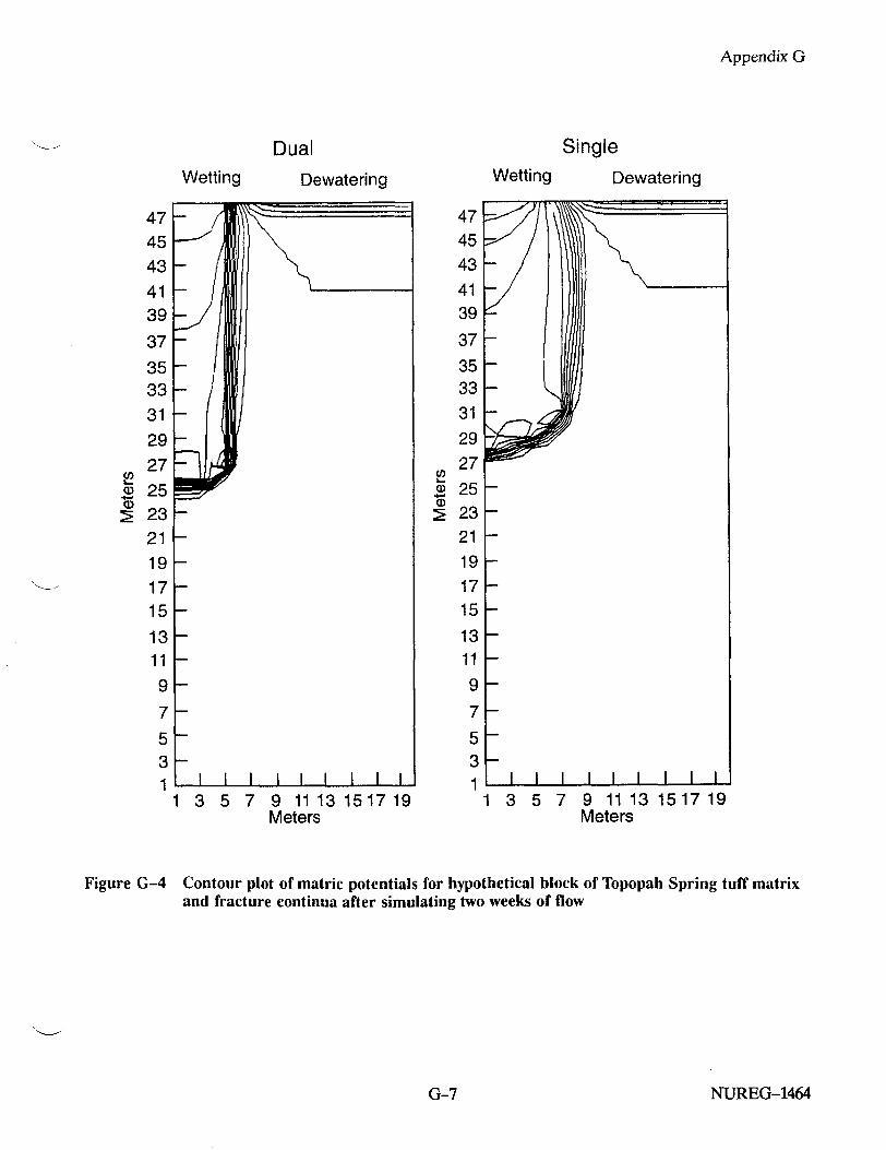
Appendix G
DualWetting Dewatering
47
45 43
41 39
37
35 33
31
29
27
25
23 21
19 17 15
13 11
9
7
5 3 1
1 3 5 7 9 11 13 15 17 19 Meters
47 45 43
41 39
37
35 33 31
29
27
25 23 21
19
17 15
13 11
9
7
5 3 1
Wetting
Single Dewatering
1 3 5 7 9 11 13 151719 Meters
Figure G-4 Contour plot of matric potentials for hypothetical block of Topopah Spring tuff matrix and fracture continua after simulating two weeks of flow
NUREG-1464
U) IQ)
4-. Q)
CO a)
2.
G-7

APPENDIX H RELEASE AND TRANSPORT OF POTENTIALLY GASEOUS RADIONUCLIDES
OTHER THAN 14C DURING VOLCANISM AND NORMAL OPERATIONS
H-1 INTRODUCTION
The Yucca Mountain site is unique among other proposed sites for the disposal of high-level radioactive waste because it would be constructed above the water table. One of the considerations at this site is radionuclide release from the waste package in the gas phase and possible transport as a gas to the atmosphere. Even if the gaseous release cannot escape to the atmosphere, it may serve as a source of contamination for the liquid pathway.
Several potentially volatile radionuclide compounds of 79Se, 991c, and 1291 have been identified in spent nuclear fuel (Lehrman, 1989; and Park, 19911). The question of whether there is sufficient cause to consider the gaseous release and transport of these volatile radionuclides further has been addressed through a series of conservative "calculations in the following sections. The direct release of the radioactive inventory by extrusive volcanism (i.e., the direct entrainment of the waste in magma brought to the surface of the earth) has been dealt with in Section 6.5. The present analysis is restricted to conditions of normal repository operation and intrusive volcanism that could potentially release volatile radionuclides from the waste package, but do not necessarily provide a mechanism for transport to the surface.
H-2 VOLATILE RELEASES RESULTING FROM THE INTRUSION OF A DIKE
To demonstrate the potential, caused by magmatic intrusion, for release of volatile radionuclides other than 14C from the engineered barrier system, consider an example of a large dike through the middle of the Yucca Mountain site. The example considers only a single dike that intrudes into the repository and does not continue to flow. The dike is represented as an instantaneous vertical plane heat source with a heat content Q per unit area (but representing a dike of finite thickness). The staff calculated the maximum
"Park, U.S., "Gaseous and Semi-Volatile Radionuclides," Unpublished Science Applications International Corporation Presentation to the U.S. Nuclear Waste Technical Review board, Denver, Colorado, June 25-27, 1991.
effect of the temperature increase at distances greater than half the assumed width of the dike, and compared the potential release of volatile radionuclides with present release limits, without specifying, at this point, a mechanistic model for the release of these components from the waste package. Although unlikely, the staff does not consider this example to be necessarily a "worst-case" situation. The example does not include the following phenomena that could lead to predictions of higher temperatures or releases:
* The formation of sills filling horizontal weakness in the rock or the repository drifts;
"* Multiple dikes and sills;
"* Long-term continuing eruptions;
"* Heat transfer by convecting gas and water vapor; and
"* Effect of corrosive volcanic gases on the waste form.
Assume for the purpose of this demonstration that a dike 10 meters in width and 3000 meters long intrudes through the middle of the repository, and that the waste packages are randomly spaced throughout the assumed site area of 5 square kilometers. Assuming that the dike intrusion is instantaneous and does not continue to the surface, the maximum range of significant heating can be determined by assuming the dissipation of heat from an infinite plane source (Turcotte and Schubert, 1982):
Q _2 T- To 2e 4 2 LC ~aic
(H-1)
where:
e = density of the country rock; C = heat capacity of country rock; Q = instantaneous sensible and latent heat
content of dike per unit area; KC = thermal diffusivity; y = distance from dike centerline;
NUREG-1464H-1

Appendix H
t TO
= time; and = ambient temperature.
The maximum temperature at any distance y from the dike centerline is (Turcotte and Schubert, 1982):
T. = T0 + Q e(H Q Cy (H-)
The time at which the maximum temperature occurs would be (Turcotte and Schubert, 1982):
tmna= - (H 2K
For the present example:
Q = 5.44 x 10⁹ Joules/square meter; @ = 2640 kilograms/cubic meter; C = 687 Joules/kilogram - degrees Kelvin
(°K); and KC 1.1 x 10⁻⁶ square meters/second
With the above set of parameters, a maximum temperature increase of 10*K would extend only 78 meters from the dike centerline and would occur only about 0.13 years after dike penetration. The 100'K isotherm would extend a maximum of 7.8 meters from the centerline.
2)
From the above analysis, the staff choose what were believed to be a very conservative maximum extent of thermal influence of the dike as 50 meters from the centerline and a 3000-meter linear extent covering an area of 300,000 square meters. The total repository area is approximately
-3) 5 x 10⁶ square meters, so the dike would affect approximately 6 percent of the waste packages. If it were conservatively assume that all of the volatile radionuclides other than 14C were driven off by the excess heat (99Tc, 79Se, and 1291) in the affected area, then the amounts in terms of the 40 CFR Part 191 (EPA, 1986) cumulative release limits would be only 0.125 as summarized in Table H-1.
Table H-I Cumulative Releases for Selected Radionuclides
EPA Limita Nuclide Inventory Curies .06 x Inventory for Repository EPA Ratio R
1291 2200 132 7000 0.019
7 9Se 28,300 1698 70,000 0.024 99Tc 915,000 54,900 700,000 0.078
Total - - 0.125
'Currently, a revised set of standards specific to the Yucca Mountain site is being developed in accordance with the provisions of the Energy Policy Act of 1992. The Energy Policy Act of 1992 (Public Law 102-486), approved October 24, 1992, directs NRC to promulgate a rule, modifying 10 CFR Part 60 of its regulations, so that these regulations are consistent with EPA's public health and safety standards for protection of the public from releases to the accessible environment from radioactive materials stored or disposed of at Yucca Mountain, Nevada, consistent with the findings and recommendations made by the National Academy of Sciences, to EPA, on issues relating to the environmental standards governing the Yucca Mountain repository. It is assumed that the revised EPA standards for the Yucca Mountain site will not be substantially different from those currently contained in 40 CFR Part 191, particularly as they pertain to the need to conduct a quantitative performance assessment as the means to estimate postclosure performance of the repository system.
NUREG-1464 H-2
Appendix H
H-3 RELEASES UNDER NORMAL CONDITIONS
Volatility of Radionuclides: Several sources of information for iodine, selenium, and technetium gave widely differing estimates of the vapor pressure. Figure H-1 shows the vapor pressure of several solid and aqueous phases of radionuclides that would occur in spent nuclear fuel, but the source of this information is unknown. Park
(1991) reports values that are considerably lower. These values are shown in Table H-2.
The vapor pressure of Tc20 7 was also estimated from thermodynamic information:
Tc2O7(solid) U Tc207 (gas)
In P = -AGO RT
NUREG-1464H-3

1 /T (10-3 OK)1
1000 500 350 250 150 100 (0C)
50 25 0 -15
1/T (10-3 OK)i
z
I
0• ON
-1
-2
-3
-4
-5
-6 S
-7
-8
-9
-10
-11
1000 500 350 250 150 100 50 25 0
(oC)
Figure H-1 Vapor pressure of several radioactive compounds (from Lehrman, 1992)
K
2
1
0
. -2 0 0) S-3
0 S.--4
-5
-6
-7
-8
-9
L -2
0) 0
0
, -4 0)
-5
-6
-7
-8
-9
-1
-2
-3
-4
-5
-6
-7
-8
-9
-10
-11
E
o2
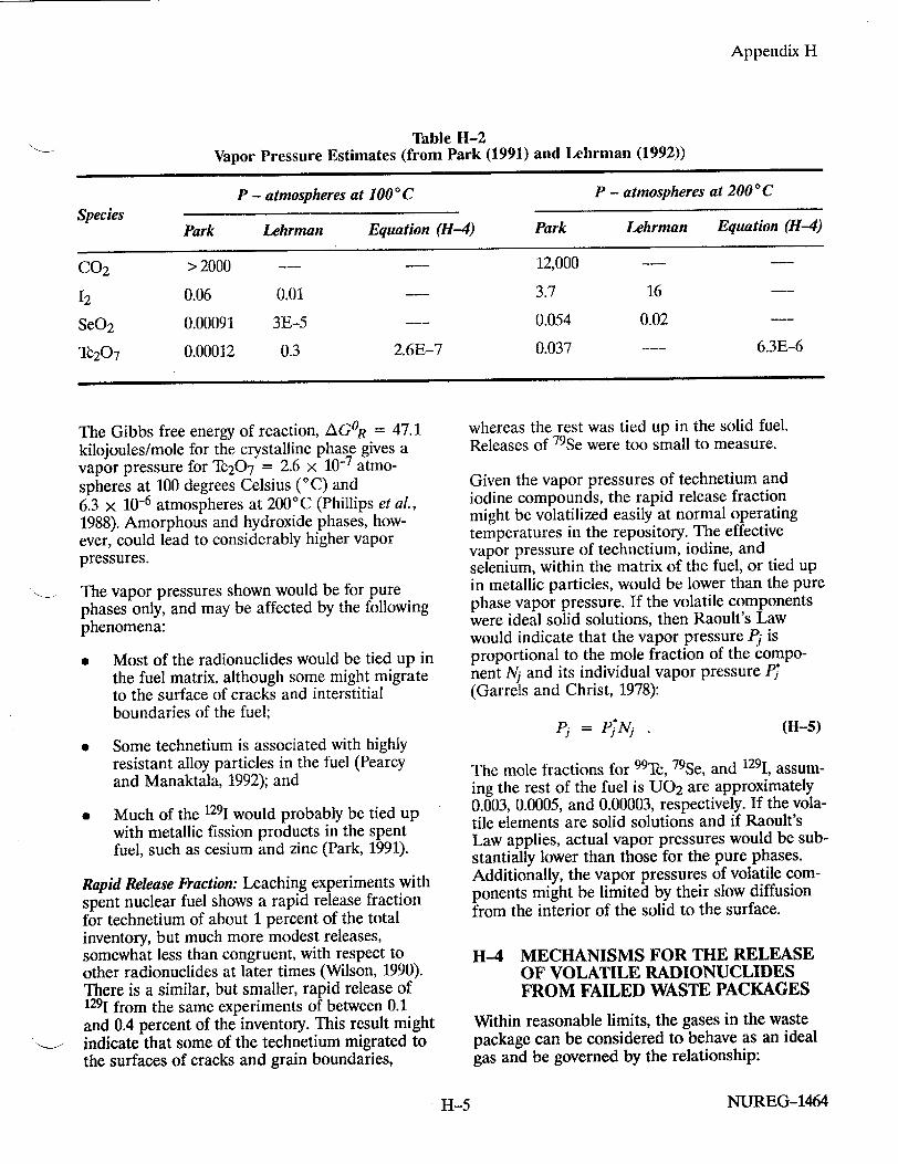
Appendix H
Table H-2 Vapor Pressure Estimates (from Park (1991) and Lehrman (1992))
P - atmospheres at 100°C P - atmospheres at 200'C
Species Park Lehrman Equation (H-4) Park Lehrman Equation (H-4)
C0 2 > 2000 --- 12,000
12 0.06 0.01 -- 3.7 16
SeO 2 0.00091 3E-5 --- 0.054 0.02 -
Tc207 0.00012 0.3 2.6E-7 0.037 6.3E-6
The Gibbs free energy of reaction, AGOR = 47.1 kilojoules/mole for the crystalline phase gives a vapor pressure for Tc2 0 7 = 2.6 x 10⁻⁷ atmospheres at 100 degrees Celsius (°C) and 6.3 x 10⁻⁶ atmospheres at 200'C (Phillips et aL, 1988). Amorphous and hydroxide phases, however, could lead to considerably higher vapor pressures.
The vapor pressures shown would be for pure phases only, and may be affected by the following phenomena:
* Most of the radionuclides would be tied up in the fuel matrix, although some might migrate to the surface of cracks and interstitial boundaries of the fuel;
* Some technetium is associated with highly resistant alloy particles in the fuel (Pearcy and Manaktala, 1992); and
Much of the 1291 would probably be tied up with metallic fission products in the spent fuel, such as cesium and zinc (Park, 1991).
Rapid Release Fraction: Leaching experiments with spent nuclear fuel shows a rapid release fraction for technetium of about 1 percent of the total inventory, but much more modest releases, somewhat less than congruent, with respect to other radionuclides at later times (Wilson, 1990). There is a similar, but smaller, rapid release of 1291 from the same experiments of between 0.1 and 0.4 percent of the inventory. This result might indicate that some of the technetium migrated to the surfaces of cracks and grain boundaries,
whereas the rest was tied up in the solid fuel. Releases of 79Se were too small to measure.
Given the vapor pressures of technetium and iodine compounds, the rapid release fraction might be volatilized easily at normal operating temperatures in the repository. The effective vapor pressure of technetium, iodine, and selenium, within the matrix of the fuel, or tied up in metallic particles, would be lower than the pure phase vapor pressure. If the volatile components were ideal solid solutions, then Raoult's Law would indicate that the vapor pressure Pj is proportional to the mole fraction of the component N) and its individual vapor pressure P; (Garrels and Christ, 1978):
Pj = PUj. (H-5)
The mole fractions for 99Tc, 7 9Se, and 1291, assuming the rest of the fuel is U0 2 are approximately 0.003, 0.0005, and 0.00003, respectively. If the volatile elements are solid solutions and if Raoult's Law applies, actual vapor pressures would be substantially lower than those for the pure phases. Additionally, the vapor pressures of volatile components might be limited by their slow diffusion from the interior of the solid to the surface.
H-4 MECHANISMS FOR THE RELEASE OF VOLATILE RADIONUCLIDES FROM FAILED WASTE PACKAGES
Within reasonable limits, the gases in the waste package can be considered to behave as an ideal gas and be governed by the relationship:
NUREG-1464H-5

Appendix H
pV = nRT, (H-6)
where:
pressure; void volume of waste package; universal gas constant; number of moles of gas; and absolute temperature.
According to Equation (H-6), the number of moles of gas n in a container of volume Vopened to the atmosphere would be directly proportional to P and inversely proportional to T. Volatile radionuclides can be released from a failed waste package by several processes, including venting of waste package pressure, molecular diffusion, and barometric pumping. Pressure within an intact waste package would depend on the initial pressure of the inert gas, release of pressurized gas within the fuel rods, partial pressure of the volatile components, and expansion of gas, because of the rise in temperature of the waste package. Upon waste package failure, the pressure would be vented, carrying with it any of the volatile radionuclides in the gas phase at that time. The fraction of the gas released An/no, assuming constant external pressure, would be:
A.n = A(T) Tno (WP-'')T
(H-7)
where To = the initial temperature at which the waste package was sealed and T' = the temperature at which it fails. Assuming that the void space in a waste package V is 300 liters, and that the inert cover gas was initially charged to the waste package at 25"C (298°K) at one atmosphere, failure of the waste package at 100*C (373"K) would release only 1 - 298/373 = 0.25 of the waste package volume or 75 liters, according to Equation (H-7).
Although molecular diffusion might be a significant effect, barometric pumping is likely to be the most important mechanism for release of volatile radionuclides, in the long term. In this case, the change in the moles of gas in the waste package is proportional to the changes in the pressure. When atmospheric pressure drops, gas
leaves the waste package, carrying with it the volatile components. In one complete cycle of pressure change AP, the fraction of gas exchanges is:
An AP no P0
(H-8)P V R n T
NUREG-1464
Atmospheric pressure changes at the surface of the earth vary on several time scales. Small, rapid pressure changes occur because of local meteorological conditions. Larger and slower changes occur because of passing weather systems. Pressure fluctuations are smaller at depth because of the resistance to gas flow through the rock and the volume of gas held in the rock. Pressure fluctuations in the unsaturated zone at Yucca Mountain are shown in Figure H-2, indicating the damping of pressure with depth (Montazer et al., 1988). Although measurements of pressure fluctuations at the repository level are not available at Yucca Mountain, assume for the sake of this example that a 1 percent fully cyclic pressure change takes place 4 times per year at the repository level. This would lead to an exchange of air within the open waste package, according to the ideal gas law, of 0.04, or 12 liters of gas per year. Over 10,000 years, this gas flow would be 1.2 x 10⁵ liters, far exceeding the initial pulse from pressure relief of the waste package.
H-5 TRANSPORT OF VOLATILE RADIONUCLIDES IN THE GEOSPHERE
The most significant volatile radionuclides other than 14C, namely Tc20 7, SeO2, and 12, are highly reactive chemically and probably will strongly favor the water contained in the unsaturated rock rather than exist as gases in the geosphere (EPA, 1993). Experience with reactor emergency spray systems shows very high removal of iodine gas in slightly alkaline water. Yucca Mountain groundwater is alkaline, leading to the tentative conclusion that most of the iodine released as a gas would transfer to the liquid phase. Escape to the atmosphere, while likely for 14C, is unlikely for the other volatile radionuclides.
Example: To demonstrate the likely maximum consequences of volatile releases of the potential gaseous radionuclides other than 14C, consider
H--6

Appendix H
0.880
0.875
Depth (m)
JJ*- 13 0.870 - -- - 19
- - - - 28
40S 39 4* 81
0.865 Feb. 26 Feb. 27 Feb. 25
1984
Figure H-2 Down-hole pressure variations at bore hole USW UZ-1 (from Montazer et aL., 1988)
the following bounding calculation. The main cause of waste package failure in the Iterative Performance assessment (IPA) Phase 2 assessment (Chapter 5) assumes that most of the waste packages will remain intact until their temperature has fallen below approximately 100'C. For the purpose of this conservative demonstration assume release of volatile radionuclides from a failed waste package under the following assumptions:
* Steady 100'C for a period of 10,000 years;
The quick-release fractions of readilyvolatilized radionuclides will be taken as 1 percent of the inventory for 99Tc, 0.4 percent of the inventory for 1291, and zero for 79Se (Wilson, 1990);
0 Vapor pressures for the pure substances at 100°C taken to be the largest values reported
in Table H-2, of 0.06 atmospheres for 1291, 0.00091 atmospheres for 79Se, and 0.3 atmospheres for 99Tc;
" The vapor pressures of the quick-release fractions are those of the pure phases;
" The remaining inventories have reduced vapor pressures according to Raoult's Law and their mole fractions in the fuel (i.e., 0.003, 0.0005 and 0.00003 for 99 Tc, 79 Se, and 1291, respectively); and
" The gas exchange during the period is 12 liters/year per waste package.
Assuming no significant radioactive decay, the rate of loss from the quick-release fraction and the solid-solution fraction depends only on the partial pressure of each component and the flow rate of the gas. For the quick release fraction, the
N NUREG-1464
Cd
-C
H--7
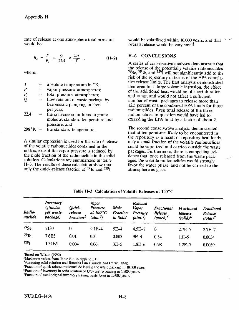
Appendix H
rate of release at one atmosphere total pressure would be:
P Q x 298 PT 22.4 T (H-9)
where:
7' = absolute temperature in 'K; P = vapor pressure, atmospheres; Pt = total pressure, atmospheres; Q = flow rate out of waste package by
barometric pumping, in liters per year;
22.4 = the conversion for liters to gram/ moles at standard temperature and pressure; and
298°K = the standard temperature.
A similar expression is used for the rate of release of the volatile radionuclides contained in the matrix, except the vapor pressure is reduced by the mole fraction of the radionuclide in the solid solution. Calculations are summarized in Table H-3. The results of these calculation show that only the quick-release fraction of 99Tc and 1291
would be volatilized within 10,000 years, and that overall release would be very small.
H-6 CONCLUSIONS
A series of conservative analyses demonstrate that the release of the potentially volatile radionuclides 79Se, 99Tc, and 1291 will not significantly add to the risk of the repository in terms of the EPA cumulative release limits. The first analysis demonstrated that even for a large volcanic intrusion, the effect of the additional heat would be of short duration and range, and would not affect a sufficient number of waste packages to release more than 12.5 percent of the combined EPA limits for those radionuclides. Even total release of the three radionuclides in question would have led to exceeding the EPA limit by a factor of about 2.
The second conservative analysis demonstrated that at temperatures likely to be encountered in the repository as a result of repository heat loads, only a small fraction of the volatile radionuclides could be vaporized and carried outside the waste packages. Furthermore, there is compelling evidence that, once released from the waste packages, the volatile radionuclides would strongly favor the water phase, and not be carried to the atmosphere as gases.
Table H-3 Calculation of Volatile Releases at 100°C
Inventory Vapor Reduced (gimoles Quick- Pressure Mote Vapor Fractional Fractional Fractional
Radio- per waste release at 1000 C Fraction Pressure Release Release Release nuclide package) Fraction2 (atm. 3) in Solid (atm. 4) (quick)s (solid)6 (total) 7
79Se 7130 0 9.1E-4 5E-4 4.5E-7 0 2.7E-7 2.7E-7 99Tc 7.6E5 0.01 0.3 0.003 9E-4 0.34 i.E-5 0.0034 1291 1.34E5 0.004 0.06 3E-5 1.8E-6 0.98 1.2E-7 0.0039
2Based on Wilson (1990). 3Maximum values from Table F-1 in Appendix F 4Assuming solid solution and Raoult's Law (Garrels and Christ, 1978). 5Fraction of quick-release radionuclide leaving the waste package in 10,000 years. "6Fraction of inventory in solid solution of U0 2 matrix leaving in 10,000 years. 7Fraction of total original inventory leaving waste form in 10,000 years.
NUREG-1464 H-8
Appendix H
H-7 REFERENCES
Garrels, R.M. and C.L. Christ, Solutions, Minerals and Equilibria, San Francisco, California, WH. Freeman, Cooper and Co., 1978.
Lehrman, A. "Volatile Radionuclides: Limiting Concentrations and Transport Rates in an Unsaturated Rock Pore Space," Lawrence Livermore National Laboratory, Chemistry and Migration Behavior of Actinides and Fission Products in the Geosphere: Abstracts of the Second International Conference on Radionculide Migration (Migration '89), November 6-10, 1989, Monterey, California, Abstract No. 2A3, p. 117.
Montazer, P., E.P. Weeks, E Thamir, D. Hammermeister, S.N. Yard, and PB. Hofrichter, "Monitoring the Vadose Zone in Fractured Tuff, Yucca Mountain, Nevada," Groundwater Monitoring Review, 8(2):72-85 [Spring 1988].
Pearcy, E.W and H.K. Manaktala, "Occurrence of Metallic Phases in Spent Nuclear Fuel: Significance for Source Term Predictions for High-Level Waste Disposal," American Nuclear Society/ American Society of Civil Engineers, Proceedings of the Third International Conference: High-Level
Radioactive Waste Management, April 12-16, 1992, Las Vegas, Nevada, 1:131-136 [19921.
Phillips, S.L., EV. Hale, L.E Silvester, and M.D. Siegal, "Thermodynamic Tables for Nuclear Waste Isolation," U.S. Nuclear Regulatory Commission, NUREG/CR-4864, June 1988.
Turcotte, D.L. and G. Schubert, Geodynamics: Application of Continuum Physics to Geological Problems, New York, J. Wiley and Sons, 1982.
U.S. Environmental Protection Agency, "Environmental Standards for the Management of Spent Nuclear Fuel, High-Level and Transuranic Wastes [Final Rule]," Federal Register, vol. 50, no. 182, September 19, 1985, pp. 38066 - 38089.
U.S. Environmental Protection Agency/Science Advisory Board, 'An SAB Report: Review of Gaseous Release of Carbon-14," Washington D.C., EPA-SAB-RAC-93-010, April 1993.
Wilson, C.N., "Results from NNWSI Series 3 Spent Fuel Dissolution Tests", Richland, Washington, Pacific Northwest Laboratories, PNL-7170, June 1990. [Prepared by the Battelle Memorial Institute.]
NUREG-1464H--9

APPENDIX I EVALUATION OF USGS GROUND-WATER MODELING FOR THE
REGION THAT INCLUDES YUCCA MOUNTAIN
I-1 INTRODUCTION
This report describes the major ground-water modeling work that has been performed by the U.S. Geological Survey (USGS) for the region of southern Nevada. Emphasis will be placed on the evolution of the subregional model originally developed by Czarnecki and Waddell (1984). This report is an auxiliary analysis under the staff's Iterative Performance Assessment effort (IPA Phase 2). Through this program, the staff is developing tools needed to review a license application for a potential high-level radioactive waste (HLW) repository.
In the late 1970's, the USGS began an appraisal of the Nevada Test Site as a potential disposal site for HLW. This work included regional geologic and hydrologic investigations, and a regional ground-water flow model was developed by "Waddell (1982). Waddell produced a twodimensional (2-D), steady-state, finite element model that covered an area of about 18,000 square kilometers. This model extended from the Pahranagat Range and Las Vegas Valley on the east to Pahute Mesa and Death Valley on the west (see Figure I-1). The model included the Yucca Mountain area and almost all of the Nevada Test Site.
Rice (1984) developed a preliminary finite difference model covering an even larger area, extending farther west and south than Waddell's (1982) model. One of the simplifying assumptions used was to simulate the flow system under confined conditions. Initial estimates of transmissivity were based on those obtained from the regional model of Waddell (1982). One of Rice's conclusions was that the model could be improved by calibrating it under unconfined conditions.
Following identification of the proposed Yucca Mountain site, Czarnecki and Waddell (1984) developed a subregional model within the hydrologic subbasin that includes the site. Thismodel was derived using a parameter estimation procedure developed by Cooley (1977, 1979, 1982). Czarnecki (1985) later revised and improved this
model to help develop smaller site-scale models of ground-water flow and transport for the Yucca Mountain site. Czarnecki initially prepared a steady-state baseline model and revised it to simulate the geohydrologic effects of increased recharge in the region. A transient version of the model was later used to evaluate scenarios related to the large hydraulic gradient located north of Yucca Mountain (Czarnecki, 1990a). Czarnecki (1992) simulated future water level declines in response to various rates of ground-water withdrawals from Wells J-13 and J-12.
Because of the importance of the USGS regional modeling work with respect to site characterization of the Yucca Mountain site, the NRC staff has acquired the subregional model of Czarnecki (1985) and the MODFE computer code. PC-based versions of the code and model have been prepared to facilitate evaluation by the staff.
This evaluation is provided below, and serves as an example of how the staff can directly obtain and evaluate numerical codes and models developed under the U.S. Department of Energy's (DOE's) HLW program. In this way the NRC staff can become more knowledgeable about codes and models during site characterization and prior to receipt of a potential license application.
1-2 REGIONAL SETTING GEOHYDROLOGY
All aspects of the geohydrologic setting must be considered when developing conceptual and numerical flow models for a site or region. The validity of a numerical model depends entirely on the validity of the conceptual model on which it is based. The conceptual flow model must reasonably represent climatic conditions, surface hydrology, hydrostratigraphy, aquifer coefficients, and recharge and discharge conditions. Chapter 3 ("Hydrology") of the Site Characterization Plan (SCP) (DOE, 1988) reports at length on past hydrogeologic work in southern Nevada. The data and interpretations contained in the 1988 SCP provide a basis for previous regional
NUREG-14641-1

Appendix I
116030, 116000, 115030' 11500'
NEVADA 0,)4G
0 2 MLE
-~~~ ~37030' ,/(0
INDEX MAP QE Al
$ ~TEST STE- A '
PAH.UTE MESA, '
~,~,#~CCCCACC4KCCC
CRATERNA AS
W elds M....t ui
36I30ian Springy.
%.a0e J61 ..... .. .. 4
PAHRUMP
0 25 50 KILOMETERS
0 25 MILES
EXPLANATION QUATERNARY
~jj~ Alluvium, lake beds, and minor volcanic rocks Lower carbonate aquifer TERTIARY PALEOZOIC (CAMBRIAN) AND PRECAMBRIAN
STuff, rhyolite. and associated volcanic rocks Lower classic aquitard MESOZOIC (Minor -- not shown) SYMBOLS
PALE OZOIC ' Contact : Undifferentiated upper classic aquitard. *- Trust fault with sawteeth on upper plate and lower and upper carbonate aquifers Regional model boundary (Waddell, 1982)
p (approximate boundary of ground-water system) SUpper classic aquitard Subregional model boundary (this report)
0 Approximate direction of ground water flow
Figure 1-1 Locations of regional and subregional modeled areas, with generalized ground-water flow directions, and generalized geology (Modified from Czarnecki and Waddell (1984, p. 2).)
NUREG-1464 1-2
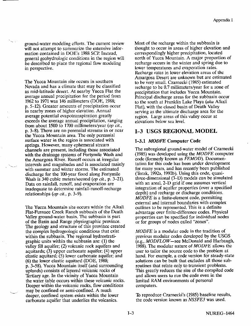
Appendix I
ground-water modeling efforts. The current review will not attempt to summarize the extensive information contained in DOE's 1988 SCP. Instead, general geohydrologic conditions in the region will be described to place the regional flow modeling in perspective.
The Yucca Mountain site occurs in southern Nevada and has a climate that may be classified as mid-latitude desert. At nearby Yucca Flat the average annual precipitation for the period from 1962 to 1971 was 146 millimeters (DOE, 1988; p. 5-12). Greater amounts of precipitation occur in nearby zones of higher elevation. Annual average potential evapotranspiration greatly exceeds the average annual precipitation, ranging from about 1500 to 1700 millimeters/year (op cit., p. 3-8). There are no perennial streams in or near the Yucca Mountain area. The only perennial surface water in the region is associated with springs. However, many ephemeral stream channels are present, including those associated with the drainage systems of Fortymile Wash and the Amargosa River. Runoff occurs at irregular intervals and magnitudes and is associated mainly with summer and winter storms. The estimated discharge for the 100-year flood along Fortymile Wash is 340 cubic meters/second (op cit., p. 3-21). Data on rainfall, runoff, and evaporation are inadequate to determine rainfall-runoff-recharge relationships (op cit., p. 3-9).
The Yucca Mountain site occurs within the Alkali Flat-Furnace Creek Ranch subbasin of the Death Valley ground-water basin. The subbasin is part of the Basin and Range physiographic province. The geology and structure of this province created the complex hydrogeologic conditions that exist within the subbasin. The regional hydrostratigraphic units within the subbasin are: (1) the valley fill aquifer; (2) volcanic rock aquifers and aquitards; (3) upper carbonate aquifer; (4) upper clastic aquitard; (5) lower carbonate aquifer; and (6) the lower clastic aquitard (DOE, 1988; p. 3-58). Yucca Mountain itself (and surrounding uplands) consists of layered volcanic rocks of Tertiary age. In the vicinity of Yucca Mountain the water table occurs within these volcanic rocks. Deeper within the volcanic rocks, flow conditions may be confined or semi-confined. A much deeper, confined system exists within the lower carbonate aquifer that underlies the volcanics.
Most of the recharge within the subbasin is thought to occur in areas of higher elevation and correspondingly higher precipitation, located north of Yucca Mountain. A major proportion of recharge occurs in the winter and spring due to lower temperatures and evaporation rates. Recharge rates in lower elevation areas of the Amargosa Desert are unknown but are estimated to be very small. Czarnecki (1985) estimated recharge to be 0.7 millimeters/year for a zone of precipitation that includes Yucca Mountain. Principal discharge areas for the subbasin occur to the south at Franklin Lake Playa (aka Alkali Flat), with the closed basin of Death Valley serving as the ultimate discharge area for the region. Large areas of this valley occur at elevations below sea level.
1-3 USGS REGIONAL MODEL
1-3.1 MODFE Computer Code
The subregional ground-water model of Czarnecki (1985) was developed using the MODFE computer code (formerly known as FEMOD). Documentation for this code has been under development for many years, and has recently been published (Torak, 1992a, 1992b). Using this code, quasithree-dimensional (3-D) models can be simulated with an areal, 2-D grid if one assumes vertical integration of aquifer properties (over a specified depth) and recharge or discharge conditions. MODFE is a finite-element code, permitting external and internal boundaries with complex outlines to be represented. This is a definite advantage over finite-difference codes. Physical properties can be specified for individual nodes or for groups of nodes called "zones".
MODFE is a modular code in the tradition of previous modular codes developed by the USGS (e.g., MODFLOW-see McDonald and Harbaugh, 1988). The modular nature of MODFE allows the user to tailor the source code to the problem at hand. For example, a code version for steady-state solutions can be built that excludes all those subroutines that relate only to transient problems. This greatly reduces the size of the compiled code and allows users to run the code even in the limited RAM environments of personal computers.
To reproduce Czarnecki's (1985) baseline results, the code version known as NSSFE3 was used.
NUREG-14641-3
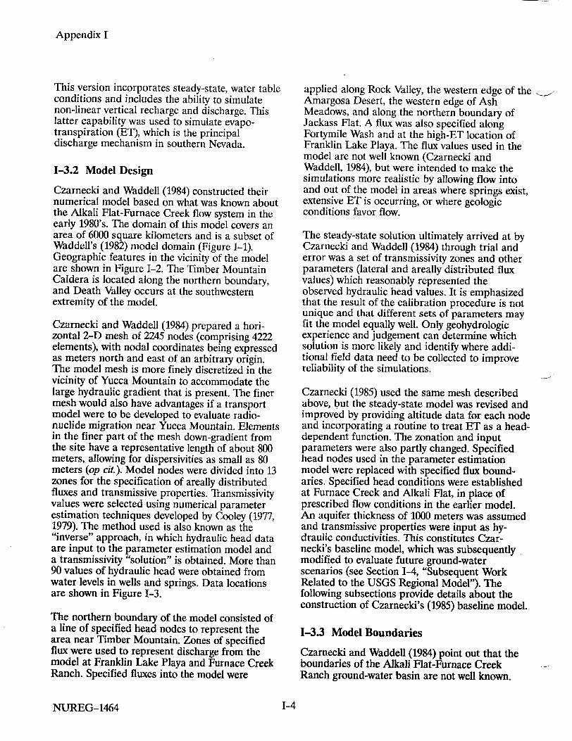
Appendix I
This version incorporates steady-state, water table conditions and includes the ability to simulate non-linear vertical recharge and discharge. This latter capability was used to simulate evapotranspiration (ET), which is the principal discharge mechanism in southern Nevada.
1-3.2 Model Design
Czarnecki and Waddell (1984) constructed their numerical model based on what was known about the Alkali Flat-Furnace Creek flow system in the early 1980's. The domain of this model covers an area of 6000 square kilometers and is a subset of Waddell's (1982) model domain (Figure 1-1). Geographic features in the vicinity of the model are shown in Figure 1-2. The Timber Mountain Caldera is located along the northern boundary, and Death Valley occurs at the southwestern extremity of the model.
Czarnecki and Waddell (1984) prepared a horizontal 2-D mesh of 2245 nodes (comprising 4222 elements), with nodal coordinates being expressed as meters north and east of an arbitrary origin. The model mesh is more finely discretized in the vicinity of Yucca Mountain to accommodate the large hydraulic gradient that is present. The finer mesh would also have advantages if a transport model were to be developed to evaluate radionuclide migration near Yucca Mountain. Elements in the finer part of the mesh down-gradient from the site have a representative length of about 800 meters, allowing for dispersivities as small as 80 meters (op cit.). Model nodes were divided into 13 zones for the specification of areally distributed fluxes and transmissive properties. Transmissivity values were selected using numerical parameter estimation techniques developed by Cooley (1977, 1979). The method used is also known as the "inverse" approach, in which hydraulic head data are input to the parameter estimation model and a transmissivity "solution" is obtained. More than 90 values of hydraulic head were obtained from water levels in wells and springs. Data locations are shown in Figure 1-3.
The northern boundary of the model consisted of a line of specified head nodes to represent the area near Timber Mountain. Zones of specified flux were used to represent discharge from the model at Franklin Lake Playa and Furnace Creek Ranch. Specified fluxes into the model were
applied along Rock Valley, the western edge of the Amargosa Desert, the western edge of Ash Meadows, and along the northern boundary of Jackass Flat. A flux was also specified along Fortymile Wash and at the high-ET location of Franklin Lake Playa. The flux values used in the model are not well known (Czarnecki and Waddell, 1984), but were intended to make the simulations more realistic by allowing flow into and out of the model in areas where springs exist, extensive ET is occurring, or where geologic conditions favor flow.
The steady-state solution ultimately arrived at by Czarnecki and Waddell (1984) through trial and error was a set of transmissivity zones and other parameters (lateral and areally distributed flux values) which reasonably represented the observed hydraulic head values. It is emphasized that the result of the calibration procedure is not unique and that different sets of parameters may fit the model equally well. Only geohydrologic experience and judgement can determine which solution is more likely and identify where additional field data need to be collected to improve reliability of the simulations.
Czarnecki (1985) used the same mesh described above, but the steady-state model was revised and improved by providing altitude data for each node and incorporating a routine to treat ET as a headdependent function. The zonation and input parameters were also partly changed. Specified head nodes used in the parameter estimation model were replaced with specified flux boundaries. Specified head conditions were established at Furnace Creek and Alkali Flat, in place of prescribed flow conditions in the earlier model. An aquifer thickness of 1000 meters was assumed and transmissive properties were input as hydraulic conductivities. This constitutes Czarnecki's baseline model, which was subsequently modified to evaluate future ground-water scenarios (see Section 1-4, "Subsequent Work Related to the USGS Regional Model"). The following subsections provide details about the construction of Czarnecki's (1985) baseline model.
1-3.3 Model Boundaries
Czarnecki and Waddell (1984) point out that the boundaries of the Alkali Flat-Furnace Creek Ranch ground-water basin are not well known.
NUREG-1464 1-4
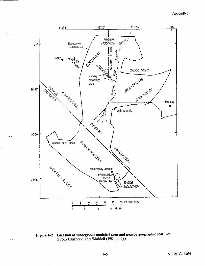
1 1 R°AK' 11 R°qO 116015'11 P5R 1V 5
/
Boundary of modeled area
Beatty -
1160
area
36045' l-
Mercury
Lathrop Walls N,1
36030' r
36015'
0
'9
-9 EAGLE MOUNTAIN
0 5 10 15 20 25 30 KILOMETERS ,, 1 I
0 5 10 15 MILES
Figure 1-2 Location of subregional modeled area and nearby geographic features (From Czarnecki and Waddell (1984, p. 6).)
NUREG-1464
370 1
Appendix I
Ii
t a
1-5

0 5 10 I P I
116030' 116015,
15 20 25 30 KILOMETERS -I- f I , I
10 15 MILES
Figure 1-3 Hydraulic head (1984, p. 13).)
and location of measurement sites (After Czarnecki and Waddell
NUREG-1464
Appendix I
116045' 1160
370
36045'
36030'
36015'
0 5| • _ I • . • i • • •
1-6
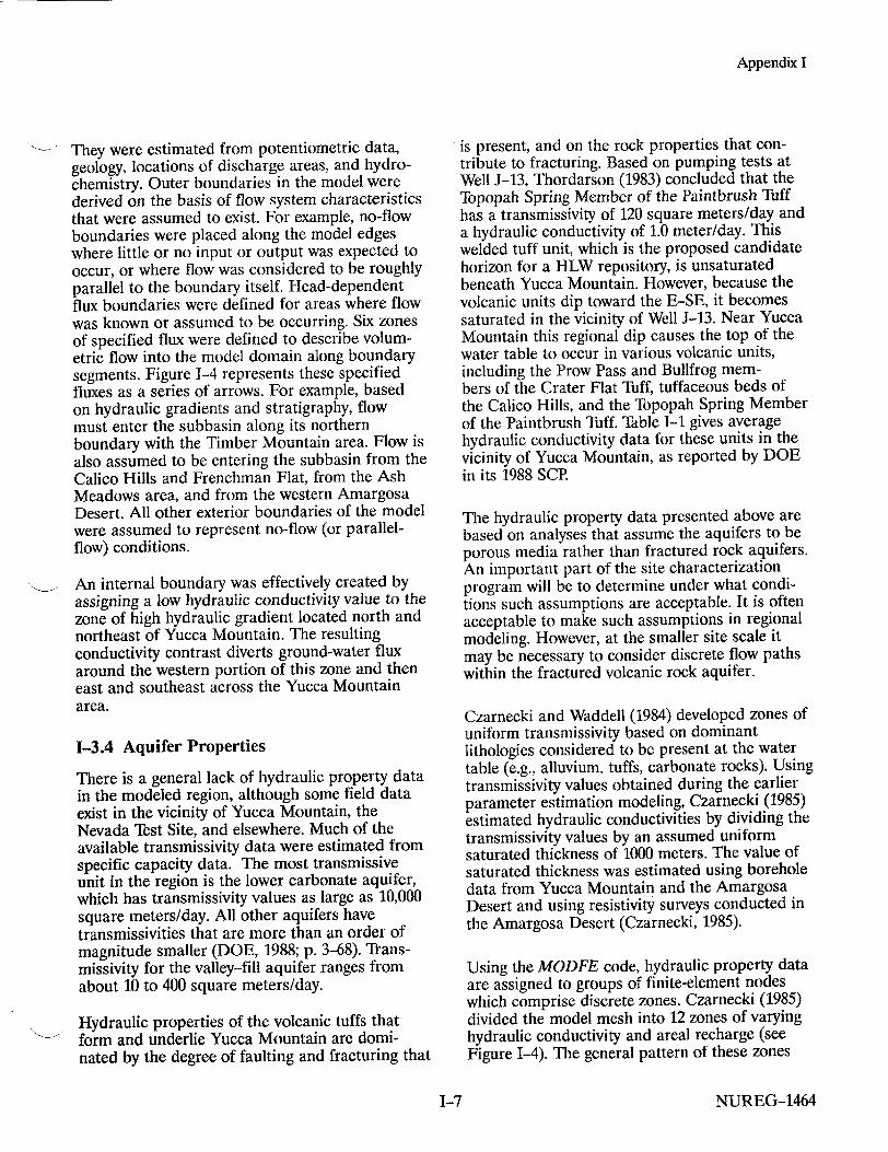
Appendix I
They were estimated from potentiometric data, geology, locations of discharge areas, and hydrochemistry. Outer boundaries in the model were derived on the basis of flow system characteristics that were assumed to exist. For example, no-flow boundaries were placed along the model edges where little or no input or output was expected to occur, or where flow was considered to be roughly parallel to the boundary itself. Head-dependent flux boundaries were defined for areas where flow was known or assumed to be occurring. Six zones of specified flux were defined to describe volumetric flow into the model domain along boundary segments. Figure 1-4 represents these specified fluxes as a series of arrows. For example, based on hydraulic gradients and stratigraphy, flow must enter the subbasin along its northern boundary with the Timber Mountain area. Flow is also assumed to be entering the subbasin from the Calico Hills and Frenchman Flat, from the Ash Meadows area, and from the western Amargosa Desert. All other exterior boundaries of the model were assumed to represent no-flow (or parallelflow) conditions.
An internal boundary was effectively created by assigning a low hydraulic conductivity value to the zone of high hydraulic gradient located north and northeast of Yucca Mountain. The resulting conductivity contrast diverts ground-water flux around the western portion of this zone and then east and southeast across the Yucca Mountain area.
1-3.4 Aquifer Properties
There is a general lack of hydraulic property data in the modeled region, although some field data exist in the vicinity of Yucca Mountain, the Nevada Test Site, and elsewhere. Much of the available transmissivity data were estimated from specific capacity data. The most transmissive unit in the region is the lower carbonate aquifer, which has transmissivity values as large as 10,000 square meters/day. All other aquifers have transmissivities that are more than an order of magnitude smaller (DOE, 1988; p. 3-68). Transmissivity for the valley-fill aquifer ranges from about 10 to 400 square meters/day.
Hydraulic properties of the volcanic tuffs that form and underlie Yucca Mountain are dominated by the degree of faulting and fracturing that
is present, and on the rock properties that contribute to fracturing. Based on pumping tests at Well J-13, Thordarson (1983) concluded that the Topopah Spring Member of the Paintbrush Tuff has a transmissivity of 120 square meters/day and a hydraulic conductivity of 1.0 meter/day. This welded tuff unit, which is the proposed candidate horizon for a HLW repository, is unsaturated beneath Yucca Mountain. However, because the volcanic units dip toward the E-SE, it becomes saturated in the vicinity of Well J-13. Near Yucca Mountain this regional dip causes the top of the water table to occur in various volcanic units, including the Prow Pass and Bullfrog members of the Crater Flat Tuff, tuffaceous beds of the Calico Hills, and the Topopah Spring Member of the Paintbrush Tuff. Table 1-1 gives average hydraulic conductivity data for these units in the vicinity of Yucca Mountain, as reported by DOE in its 1988 SCP.
The hydraulic property data presented above are based on analyses that assume the aquifers to be porous media rather than fractured rock aquifers. An important part of the site characterization program will be to determine under what conditions such assumptions are acceptable. It is often acceptable to make such assumptions in regional modeling. However, at the smaller site scale it may be necessary to consider discrete flow paths within the fractured volcanic rock aquifer.
Czarnecki and Waddell (1984) developed zones of uniform transmissivity based on dominant lithologies considered to be present at the water table (e.g., alluvium, tuffs, carbonate rocks). Using transmissivity values obtained during the earlier parameter estimation modeling, Czarnecki (1985) estimated hydraulic conductivities by dividing the transmissivity values by an assumed uniform saturated thickness of 1000 meters. The value of saturated thickness was estimated using borehole data from Yucca Mountain and the Amargosa Desert and using resistivity surveys conducted in the Amargosa Desert (Czarnecki, 1985).
Using the MODFE code, hydraulic property data are assigned to groups of finite-element nodes which comprise discrete zones. Czarnecki (1985) divided the model mesh into 12 zones of varying hydraulic conductivity and areal recharge (see Figure 1-4). The general pattern of these zones
NUREG-14641-7
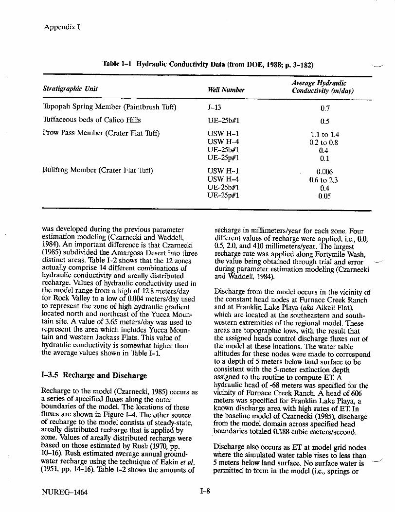
Appendix I
Table I-1 Hydraulic Conductivity Data (from DOE, 1988; p. 3-182)
Average Hydraulic Stratigraphic Unit Well Number Conductivity (m/day)
Topopah Spring Member (Paintbrush Tuff) J-13 0.7
Tuffaceous beds of Calico Hills UE-25b#1 0.5
Prow Pass Member (Crater Flat Tuff) USW H-1 1.1 to 1.4 USW H-4 0.2 to 0.8 UE-25b#1 0.4 UE-25p#1 0.1
1Billfrog Member (Crater Flat Tuft) USW H-1 0.006 USW H-4 0.6 to 2.3 UE-25b#1 0.4 UE-25p#1 0.05
was developed during the previous parameter estimation modeling (Czarnecki and Waddell, 1984). An important difference is that Czarnecki (1985) subdivided the Amargosa Desert into three distinct areas. Table 1-2 shows that the 12 zones actually comprise 14 different combinations of hydraulic conductivity and areally distributed recharge. Values of hydraulic conductivity used in the model range from a high of 12.8 meters/day for Rock Valley to a low of 0.004 meters/day used to represent the zone of high hydraulic gradient located north and northeast of the Yucca Mountain site. A value of 3.65 meters/day was used to represent the area which includes Yucca Mountain and western Jackass Flats. This value of hydraulic conductivity is somewhat higher than the average values shown in Table I-1.
1-3.5 Recharge and Discharge
Recharge to the model (Czarnecki, 1985) occurs as a series of specified fluxes along the outer boundaries of the model. The locations of these fluxes are shown in Figure 1-4. The other source of recharge to the model consists of steady-state, areally distributed recharge that is applied by zone. Values of areally distributed recharge were based on those estimated by Rush (1970, pp. 10-16). Rush estimated average annual groundwater recharge using the technique of Eakin et al. (1951, pp. 14-16). Table 1-2 shows the amounts of
recharge in millimeters/year for each zone. Four different values of recharge were applied, i.e., 0.0, 0.5, 2.0, and 410 millimeters/year. The largest recharge rate was applied along Fortymile Wash, the value being obtained through trial and error during parameter estimation modeling (Czarnecki and Waddell, 1984).
Discharge from the model occurs in the vicinity of the constant head nodes at Furnace Creek Ranch and at Franklin Lake Playa (aka Alkali Flat), which are located at the southeastern and southwestern extremities of the regional model. These areas are topographic lows, with the result that the assigned heads control discharge fluxes out of the model at these locations. The water table altitudes for these nodes were made to correspond to a depth of 5 meters below land surface to be consistent with the 5-meter extinction depth assigned to the routine to compute ET A hydraulic head of -68 meters was specified for the vicinity of Furnace Creek Ranch. A head of 606 meters was specified for Franklin Lake Playa, a known discharge area with high rates of ET In the baseline model of Czarnecki (1985), discharge from the model domain across specified head boundaries totaled 0.188 cubic meters/second.
Discharge also occurs as ET at model grid nodes where the simulated water table rises to less than 5 meters below land surface. No surface water is permitted to form in the model (i.e., springs or
NUREG-1464 I-8

116045, 116030' 116015' 116
70 Boundary oi modeled area
Qfm
Beatty O
Primary repository area 1rv
I v 7 5' N.,''.•,
5-9 V • / Mercun
EXPLANATION 2 TRANSMISSIVITY ZONE
From Czarnecki and
Waddell (1984)
0 606 POINT OF CONSTANT
0 68 \HYDRAULIC HEAD, IN Ojf METERS ABOVE OR
12 \m •BELOW (-) SEA LEVEL
SPECIFIED FLUX i Qjf Jackass Flats
Qrv Rock Valley Qam Ash Meadows Owad Western Amargosa
Desert "3 Qtm Timber Mountain
Qfm Fortymile Wash \606 (areally distributed \, over zone 8)
0 5 10 15 20 25 30 KILOMETERS I i I , II I ~ I I
0 5 10 15 MILES
Figure 1-4 Model boundary fluxes, constant-head nodes, and transmissivity zones (From Czarnecki (1985, p. 7).)
NUREG-1464
Appendix I
O
1-9
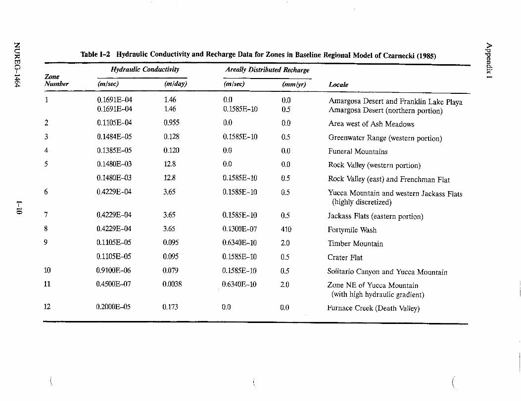
Table 1-2 Hydraulic Conductivity and Recharge Data for Zones in Baseline
Hydraulic Conductivity Areally Distributed Recharge
(misec) (m/day) (m/sec) (mm/yr)
0.1691E-04 1.46 0.0 0.0 0.1691E-04 1.46 0.1585E-10 0.5
0.1105E-04 0.955 0.0 0.0
0.1484E-05 0.128 0.1585E-10 0.5
0.1385E-05 0.120 0.0 0.0
0.1480E-03 12.8 0.0 0.0
0.1480E-03 12.8 0. 1585E- 10 0.5
0.4229E-04 3.65 0.1585E-10 0.5
0.4229E-04
0.4229E-04
0.1105E-05
0.1105E-05
0.9100E-06
0.4500E-07
3.65
3.65
0.095
0.095
0.079
0.0038
0.1585E-10
0.1300E-07
0.6340E-10
0.1585E-10
0.1585E-10
0.6340E-10
0.5
410
2.0
0.5
0.5
2.0
0.173 0.0 0.0
Zone Number
1
2
3
4
5
6
0 7
8
9
10
11
Regional Model of Czarnecki (1985)
Locale
Amargosa Desert and Franklin Lake Playa
Amargosa Desert (northern portion)
Area west of Ash Meadows
Greenwater Range (western portion)
Funeral Mountains
Rock Valley (western portion)
Rock Valley (east) and Frenchman Flat
Yucca Mountain and western Jackass Flats (highly discretized)
Jackass Flats (eastern portion)
Fortymile Wash
Timber Mountain
Crater Flat
Solitario Canyon and Yucca Mountain
Zone NE of Yucca Mountain (with high hydraulic gradient)
Furnace Creek (Death Valley)12 0.2000E-05

Appendix I
creeks). Wherever the simulated water table rises to the land surface, it is discharged entirely as ET
To treat ET in the model, a value for land surface altitude had to be assigned to each node. This information was used by the model subroutine that simulates ET as a non-linear vertical discharge per unit area. This was an important improvement introduced by Czarnecki (1985) over the previous version of this model (Czarnecki and Waddell, 1984), providing a reference altitude for each node to compare with computed water table altitudes. An "extinction" depth of 5 meters was assigned; this was considered the maximum depth from which bare-soil evaporation could occur. During a simulation, ET would occur whenever the simulated water level at a node rose to a depth of less than 5 meters. The ET coefficient used was 0.864 meters/day per unit area at land surface. This very large ET rate was used to prevent the simulated water table from rising above the surface. It also removed water from the model area that might have left through runoff. The ET rate decreased linearly to zero at the extinction depth of 5 meters below land surface (Czarnecki, 1985). Thus, the maximum ET would occur for simulated heads at land surface, and all of the discharge would be treated as ET rather than allowing the creation of surface water bodies like springs and streams.
Discharge data are available for springs in the Furnace Creek Ranch area. Some of the springs occur several hundred meters above the floor of Death Valley. Discharges in this area were estimated at 0.2 cubic meters/second (Waddell, 1982). DOE (1988, Tables B-3-B-5) lists data for more than 20 spring outlets (plus numerous seeps and phreatophyte areas) in the Furnace Creek Ranch area. For those springs for which discharge was determined, the combined discharge totals more than 0.15 cubic meters/second. This is a minimum discharge because it does not include the many seeps and phreatophyte areas in the vicinity. Czarnecki and Waddell (1984) attribute a total discharge flux of 0.22 cubic meters/second to the Furnace Creek Ranch area.
Walker and Eakin (1963) estimated discharge by ET from Franklin Lake Playa to be -0.4 cubic meters/second. Czarnecki (1990b) estimated an average volumetric discharge rate of -0.26 cubic meters/second based on field studies at the playa
(June 1983 to April 1984). Using Czarnecki's estimate, the ET discharge from this playa, when combined with estimated spring discharges in the region near Furnace Creek (-0.2 cubic meters/ second (Waddell, 1982)), yields a total discharge at these locations of about -0.4 to -0.5 cubic meters/second. This can be compared with the simulated steady-state discharges for these areas obtained using Czarnecki's (1985) model. The combined discharge across specified-head boundaries at Franklin Lake Playa and Furnace Creek Ranch is -0.19 cubic meters/second. The nonlinear routine that calculates ET yields a discharge of -0.27 cubic meters/second. The total simulated discharge occurring in the vicinity of Franklin Lake Playa and Furnace Creek Ranch is approximately -0.46 cubic meters/second.
There is apparent agreement between the observed and simulated discharges in the southern part of the model. However, the estimated spring and ET discharges do not include ground-water underflow which may exit the subbasin in these areas. For example, a significant amount of discharge likely occurs through the alluvial sediments that underlie the Amargosa River. This river basin hydrologically connects the Amargosa Desert to Death Valley, even when no surface water is flowing. The course of the ephemeral Amargosa River eventually descends into Death Valley, with a terminus at Badwater Basin (the lowest topographic basin in the U.S.). Some ground-water underflow may also occur beneath the Greenwater and Funeral Mountains via the Paleozoic carbonate aquifer. Further discussion about the discharges in the southern part of the model may be moot given the new conceptual model of flow that includes a possible flow divide in the Greenwater Range (see discussion later in this review).
Czarnecki and Waddell (1984) had previously determined that simulated rates of ET at Franklin Lake Playa had the largest effect (of all the model-boundary conditions) on estimated values for aquifer transmissivity at Yucca Mountain. Therefore, ET estimates for the playa had to be better defined. Czarnecki (1990b) documents an extensive program of field investigations at Franklin Lake Playa between June 1983 and April 1984. The playa shows extensive evidence of ground-water discharge. It is characterized by salt pan and porous surfaces, phreatophytes, very shallow ground water, and upward vertical
NUREG-14641-11

Appendix I
gradients that greatly exceed horizontal hydraulic gradients. In general, the ET rate depends on the types and density of phreatophytes, depth to the water table, ground-water salinity, soil-moisture properties, and climatic conditions (Czarnecki, 1990b). Czarnecki estimated rates of ET (centimeters/day) using various approaches, including energy-balance eddy correlation and analyses of temporal changes in soil moisture content, temperature profiles, vertical gradients in the saturated zone, and others. He concluded that the eddy correlation technique gave the most reliable estimates for ET because it is the most direct method. Czarnecki reported an estimated ET range of 38 to 41 centimeters/year at Franklin Lake Playa for 1983-84.
1-3.6 Model Results
Czarnecki (1985) obtained a baseline, steady-state solution of simulated hydraulic heads for the subbasin (see Figure 1-5). Compared to the solution from the parameter-estimation model of Czarnecki and Waddell (1984), the model results showed a decrease in the range of head residuals (-18.9 to + 21.0 meters) and a reduced estimated sum-of-squared errors for observed-versuscalculated hydraulic heads (4101 square meters). However, these comparisons may not have much meaning because the observed hydraulic head data are concentrated in areas that have small hydraulic gradients (e.g., the Amargosa Desert). Data are needed in areas where water table elevations change more rapidly (e.g., Furnace Creek area, and the region north and west of Yucca Mountain). Figure 1-6 shows the vertically integrated ground-water flux vectors in the vicinity of the Yucca Mountain site for the baseline simulation.
1-3.7 Model Sensitivity and Stability
Modeling studies by Waddell (1982) and Czarnecki and Waddell (1984) showed recharge to be a highly sensitive element of their regional flow models. In particular, the recharge value applied to Fortymile Wash had a strong influence over the simulated heads at nearby Yucca Mountain. The solution was also found to be very sensitive to the rate of ET at Franklin Lake Playa.
Czarnecki (1985) reported instability problems with the model that were probably caused by the nonlinear routine in MOI)FE that handles ET It is known that nonlinear routines can cause instability problems in numerical solutions (Roache, 1973). Significant mass-balance errors resulted when extinction depths of less than 5 meters were specified. Discretization errors may be produced by the presence of obtuse angles within the triangular elements of the finiteelement mesh (Torak, 1992a). The finite-element mesh prepared by Czarnecki and Waddell (1984) contains 4222 elements. The mesh was analyzed with a BASIC routine and found to contain almost 600 elements that include obtuse angles. For a more accurate numerical solution, all angles within the triangular elements should be acute.
In independent simulations, the NRC staff found that Czarnecki's modeling results could be reproduced using 386 and 486 personal computers equipped with WEITEK math 'coprocessors. Serious instability problems caused by round-off errors arose when running the model on computers equipped with another type of math coprocessor. The problem was corrected by specifying floating point double precision (DECLARE ALL REAL*8) in each subroutine of the FORTRAN source code. Of course, the use of double precision greatly increases the memory (RAM) required to run the model.
1-4 SUBSEQUENT WORK RELATED TO THE USGS REGIONAL MODEL
1-4.1 Modeling of the Alkali Flat-Furnace Creek Ranch Subbasin
Czarnecki (1985) investigated the possible effects on the water table of a wetter future climate. He revised the baseline model to simulate the effects of increased recharge in the region. Both recharge amounts and lateral fluxes were increased, resulting in water table rises at the Yucca Mountain site. Based on this model, Czarnecki concluded that a 100 percent increase in precipitation caused the simulated position of the water table at Yucc= Mountain to rise as much as 130 meters. This degree of water table rise would not be enough to flood a hypothetical repository in the 'Ibpopah
NUREG-1464 1-12
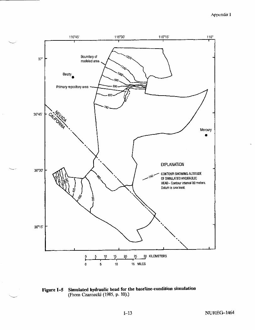
116045' 116030' 116015'
CONTOUR SHOWING ALTITUDE OF SIMULATED HYDRAULIC HEAD - Contour Interval 80 meters. Datum is sea level.
36o15' t-
0 5 10 15 20 25 30 KILOMETERS i i I1 I
o 10 15 MILES
Simulated hydraulic head for the baseline-condition simulation (From Czarnecki (1985, p. 10).)
N3NUREG-1464
370 °
Appendix I
36045'
36030' F
Figure 1-5
1160I I
9
1-13
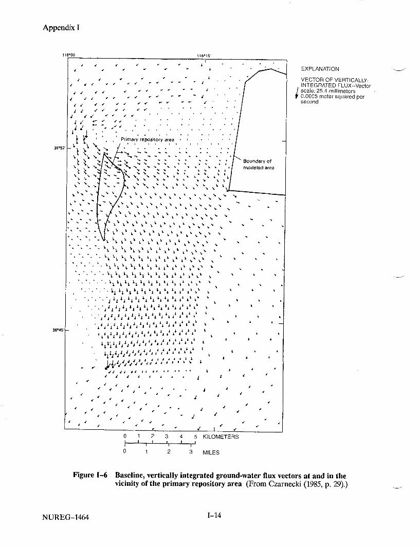
Appendix I
116'00'
e I I I I
j W V e v
6 4 %. %. , . oono ,-o
"J. ' ".: 6 ,' ,
• . ., , .j •t .' ' ••• * • •
L &I %
44 4 1
4' 44 4
44 A
.4 '
4 4 4 4 4 4 4 4 4 4 4 a & I & 4 t
- '4 4 4 4 4 4jA 4 4 4 A4 4 44
* 4 4r 4 4 4
4 4
4 4
4 4 .t
1 d
4 If I
4 4
4
4 - �1
j4
/
4, - 'a'
I
.1
4,
0 1 2 3 4 5 KILOMETERS I I I I
0 1 2 3 MILES
EXPLANATION
VECTOR OF VERTICALLYINTEGRATED FLUX--Vector s cale: 25.4 millimeters 0.0005 meter squared per second
Figure 1-6 Baseline, vertically integrated ground-water flux vectors at and in the vicinity of the primary repository area (From Czarnecki (1985, p. 29).)
NUREG-1464 1-14
116D15"
36*52.
36*45'
116-15'
J
I
I
Appendix I
Spring Member of the Paintbrush Tuff. However, the simulated water table rise would greatly reduce the thickness of the unsaturated zone and would be sufficient to cause springs to form south and west of Timber mountain, along Fortymile Wash, in the Amargosa Desert near Lathrop Wells and Franklin Lake Playa, and near Furnace Creek Ranch in Death Valley.
Czarnecki (1985) noted that the future water table rise due to a wetter climate (and increased recharge) may be exaggerated because surface water runoff was not permitted in the model. All discharges from the model occurred as either ET or lateral ground-water flow. However, it is noted that the future simulations were derived by revising a baseline model that had assumed zero modern-day recharge over large areas of the model domain. It is not yet known whether the recharge assumptions used in the baseline model are reasonable (see discussion under "Revised Conceptual Model, Section 1-4.3").
There is evidence that the water table at Yucca Mountain was significantly higher in the past. Marshall et al. (1993) describe strontium isotopic evidence for a higher water table at Yucca Mountain. They conclude that the water table may have been about 85 meters higher in the past. This degree of water table rise is of the same order of magnitude as that predicted by Czarnecki (1985) under wetter climatic conditions. This is significant with respect to performance of a potential repository. Any long-term rise of the water table over the next 10,000 years would reduce the thickness of the unsaturated zone beneath the repository. This portion of the unsaturated zone is considered the key barrier within the natural system.
Other evidence of a higher water table in the Yucca Mountain region is provided by Quade et al. (1995). They describe a group of spring deposits, informally named the Lathrop Wells diatomites, located about 20 kilometers southwest of the Yucca Mountain site. The diatomites represent fluvial and shallow aquatic environments, and are similar to other spring deposits. Although the age of the deposits is still under study, fossils of horse, camel, mammoth, and rabbit confirm that parts of them date to the Pleistocene. The position of the Lathrop Wells diatomites, relative to the modern water table,
suggests that the water table was formerly no more than 115 meters higher than it is today (op cit., p. 227).
There is also evidence that a perennial water source existed in Fortymile Canyon near Yucca Mountain during the Wisconsin glacial stage. Spaulding (1994, p. 40) concluded that plant macrofossils from a packrat midden site in Fortymile Canyon provide unequivocal evidence that a
perennial water source existed there approximately 47,000 years before the present (ybp) (and possibly earlier). This midden site, designated FMC-7, is located about 13 kilometers northeast of Yucca Mountain adjacent to Fortymile Canyon (in Area 29 of the Nevada Test Site). The site is north of the zone of high hydraulic gradient in an
area where the water table is presently much shallower than at Yucca Mountain. FMC-7 occurs at an elevation of 1250 meters, about 75 meters above the current drainage of Fortymile Canyon. The location of midden site FMC-7, along with its macrofossil and pollen assemblages, led Spaulding (1994) to conclude that the water table was at least 75 meters higher during the Early or EarlyMiddle Wisconsin (ca. 73,000 to 47,000 ybp). He
found it likely that the bed of Fortymile Canyon was 75 to 95 meters higher than today, with 65 meters of alluvium having been removed by stream incision approximately 18,500 ybp. Spaulding (1994, p. 50) provided recommendations for
future paleoecological research, noting the ".... contrast between the widely held belief that the last glacial maximum [ca. 18,000 ybpl was a time
of maximum water-table rise and spring discharge, and the utter lack of stratigraphic evidence for spring discharge during that time...."
Czarnecki (1990a) developed a transient version of his model to investigate phenomena like the large hydraulic gradient located north of the site. In one scenario, a postulated hydrologic barrier was disrupted and large volumes of ground water were released to flow southward. Such a scenario could arise due to faulting associated with an earthquake. This scenario caused a maximum rise of about 40 meters in the simulated water level at Yucca Mountain (National Research Council, 1992 (citing personal communication with J. Czarnecki)).
Czarnecki (1992) simulated water level declines in the Yucca Mountain area in response to future ground-water withdrawals from Wells J-13 and
NUREG-14641-15

Appendix I
J-12, located about 7 kilometers southeast of the Yucca Mountain site. This work is very important because it represents a 10-year forecast of how future ground-water levels will be affected by human activities. This work supported a request from DOE to the State of Nevada for a permit to pump up to 5.7 x 10⁻³ cubic meters/second from Well J-13 (op cit.). DOE requested the water to support site characterization work at Yucca Mountain over the next 10 years. Eight different pumping scenarios were analyzed using a transient version of Czarnecki's 1985 model and various combinations of withdrawal rates. Four of the scenarios involved pumping from a single well, while both wells were pumped in the other four scenarios. For each withdrawal rate, simulations were made with aquifer specific yields set at 0.001, 0.005, and 0.01. Czarnecki (1992) considered a specific yield of 0.01 to be the value that is best supported by available data. The most extreme scenario represented the combined maximum pumping capacities from both wells (8.771 x 10⁻² cubic meters/second) and assumed an aquifer specific yield of 0.001. This resulted in a drawdown of over 12.2 meters at both Wells J-12 and J-13 at the end of the 10-year period. Under the same pumping conditions, and assuming a specific yield of 0.01, simulated drawdowns at Wells J-13 and J-12 were about 3.0 meters and varied from 1.8 to 2.4 meters at the Yucca Mountain site. The simulated drawdown for the anticipated withdrawal rate of 5.7 x 10- 3 cubic meters/second from Well J-13 (based on a 10-year pumping period and a specific yield of 0.01) was 0.29 meters at Well J-13. The drawdown at the Yucca Mountain site would be about 0.2 It is expected that one of the many scenarios analyzed by Czarnecki (1992) will be representative of actual ground-water withdrawals during site characterization and can be used to test how well the regional model represents the flow system.
Oatfield and Czarnecki (1989) analyzed drillers' logs and data from geophysical surveys to identify areas in the Amargosa Desert that have relatively higher or lower transmissivities. They concluded, based on drillers' logs, that the thick alluvial deposits cannot easily be subdivided into correlative stratigraphic units. However, the drillers' logs suggested a trend of increasing consolidation of sediments from north to south. Hydrogeologic interpretation of a resistivity (vertical electric sounding) survey was complicated by a lack of
information about aquifer properties and ground water quality at depth. However, high resistivity values in the upper 75 meters of alluvium were interpreted to coincide with relatively fresh, shallow ground water that may enter the Amargosa Desert via the Fortmile Wash drainage system.
1-4.2 The Szymanski Hypothesis
Szymanski (1989) asserted that ground water at Yucca Mountain had risen to repository level repeatedly in the past, primarily because of tectonic processes. This assertion was based largely on Szymanski's hydrothermal interpretation of the origin of fracture-cementing carbonates and silica exposed in Trench 14. This trench was excavated across the Bow Ridge fault just east of Yucca Mountain. Contrary to Szymanski's interpretation of Trench 14, Quade et al. (1995, p. 228) observed that many years of scrutiny by different researchers (including themselves) have ".... failed to identify unequivocal paleospring deposits adjacent to Yucca Mountain. .... " Based on their study of modern and fossil spring deposits in the region, they found that the mineralogy of Trench 14 has no modern analog. Quade et al. concluded that morphologically, mineralogically, and isotopically, ".... the fracture carbonates in Trench 14 closely resemble pedogenic carbonate in the region.... ." (op cit.)
Before the work of Quade et al. (1995), a panel of the National Research Council (1992) had evaluated the potential for future rises of the water table to occur at Yucca Mountain. The panel assessed the likelihood that the water table could rise to the height of the repository horizon by any plausible geological process, or whether such a rise had occurred in the past. The panel cited the previous work of Waddell and Czarnecki, and emphasized the importance of field evidence in establishing the presence of past discharge areas.
With respect to earthquakes, the National Research Council Panel (1992, p. 124) concluded that "... while there are uncertainties in current interpretations because specific site data are not available, . . . there is nevertheless sufficient confidence in the aseismicity of the site and in the inability of earthquakes to generate large water table changes at the site ... to warrant further characterization of the site to determine its suitability ..... The panel recommended that the
NUREG-1464 1-16

Appendix I
"DOE conduct a literature search regarding the hydrologic effects of historic earthquakes, locally and worldwide, to determine the potential for large water table rises in response to the coupling of seismic and hydrologic systems.
The earthquake that occurred near Little Skull Mountain on June 29, 1992 (magnitude 5.6) caused only a minor, transient change in the water table at the Yucca Mountain site. The maximum fluctuation of the water table at the site was estimated at only 0.4 meters (O'Brien and Tucci, 1992). The data were obtained from two wells instrumented to continuously monitor fluctuations in the water table and fluid-pressure in a deeper, isolated interval. Water table fluctuations of similar magnitude were caused by more distant and more powerful earthquakes. Two major earthquakes occurred in southern California on June 28, 1992. Both were about 300 kilometers from Yucca Mountain and were measured as having magnitudes of 7.5 (Landers) and 6.6 (Big Bear Lake). The Landers and Big Bear Lake quakes caused estimated water table fluctuations of 0.9 meters and 0.2 meters, respectively (op cit.).
1-4.3 Revised Conceptual Model
New ideas about regional flow in the subbasin were presented and documented by Czarnecki (1987, 1989) and Czarnecki and Wilson (1989). The previously accepted conceptual model of the regional ground-water system assumed that flow beneath the central Amargosa Desert ultimately discharges from two major areas: Furnace Creek Ranch and Franklin Lake Playa. In the baseline model of Czarnecki (1985), zero recharge was assumed to be occurring over most of the subregion south of Yucca Mountain. New data were obtained by Czarnecki (1989) which led to an alternate conceptual model of subregional flow. Potentiometric data were obtained from mining property boreholes in the Greenwater Range (between Death Valley and the Amargosa Desert). These data show a water table altitude in that area of about 875 meters (Figure 1-7), providing evidence of significant ground-water recharge and the probable presence of a ground-water flow divide beneath this range. The data suggest that flow divides beneath the Greenwater and Funeral Mountains may isolate the water table aquifer in the Amargosa Desert from the flow system in
Death Valley. Geographic features of this area are illustrated in Figure 1-8.
The inclusion of flow divides beneath the Greenwater and Funeral Mountains is a major revision of the conceptual model used to develop Czarnecki's regional flow model, in that the discharge area at Furnace Creek Ranch may be relatively isolated from the water table aquifer underlying the Amargosa Desert. Instead, Franklin Lake Playa may serve as the principal discharge area for the subregional water table flow system that includes Yucca Mountain, and discharge at Furnace Creek Ranch may be derived primarily from the confined carbonate aquifer. Winograd and Thordarson (1975) had previously suggested this possibility, based on the proximity of spring discharge to the lower carbonate aquifer and temperature and hydrochemical conditions (DOE, 1988; p. 3-79). A portion of the discharge at Furnace Creek Ranch may also be derived from recharge in the nearby mountains. To help confirm the new conceptual model, a number of wells would be needed to better define hydraulic heads in the ground-water divide areas north and east of Furnace Creek Ranch. DOE (1990, p. 3.2-6) describes plans to drill new wells, including one planned for the eastern edge of the Funeral Mountains. Figure 1-7 shows Czarnecki's proposed revision of the flow system with inferred water-level contours based on the data from the Greenwater Range and a principal discharge area at Franklin Lake Playa.
As discussed in Czarnecki and Wilson (1989), a revised conceptual model for the subbasin would include the following:
" The presence of a regional Paleozoic carbonate aquifer which underlies the subbasin that includes Yucca Mountain;
" Upward flow originating from the carbonate aquifer occurs from great depths within the subbasin;
" Spring flow in Death Valley near Furnace Creek Ranch is from the carbonate aquifer, which forms a confined aquifer that is separate from the overlying water table system; and
"* Some recharge to the ground-water system may be occurring even in arid areas such as
N7NUREG-14641-17

Appendix I
the Funeral Mountains and the Greenwater Range.
The revised conceptual model is significant in that it would require less volumetric flow through the region that includes Yucca Mountain. Other conditions being equal, this means that simulated ground-water velocities would generally be less than in the original model. But it also suggests that the flow system may be more susceptible to future large-scale stresses such as extensive ground-water overdrafts.
1-4.4 Site Characterization Study Plans
In support of the Yucca Mountain project, DOE has developed study plans that outline a program for characterizing and modeling the regional flow system. DOE (1990) describes plans to characterize the regional ground-water flow system. The study, "Regional Hydrologic Synthesis and Modeling" (DOE, 1991), will analyze regional ground-water data, formulate conceptual models of the regional flow system, and develop and calibrate numerical models. Other study plans, such as those involving climatology, geochemistry, and geology, are also related to the characterization and modeling of the ground-water system. Results of the regional modeling will be used to specify boundary conditions for site-scale models of the saturated zone at Yucca Mountain. Regional models will also be used to estimate changes in the regional (and local) ground-water system caused by future climatic conditions, human activities, and tectonic events. In this way the modeling results are intended to support site-scale evaluations of repository performance with respect to the NRC's criterion for ground-water travel time (10 CFR 60.113(aX2)) and the EPA standards under 40 CFR Part 191.1
'Currently, a revised set of standards specific to the Yucca Mountain site is being developed in accordance with the provisions of the Energy Policy Act of 1992. The Energy Policy Act of 1992 (Public Law 102-486), approved October 24, 1992, directs NRC to promulgate a rule, modifying 10 CFR Part 60 of its regulations, so that these regulations are consistent with EPA's public health and safety standards for protection of the public from releases to the accessible environment from radioactive materials stored or disposed of at Yucca Mountain, Nevada, consistent with the findings and recommendations made by the National Academy of Sciences, to EPA, on issues relating to the environmental standards governing the Yucca Mountain repository. It is assumed that the revised EPA standards for the Yucca Mountain site will not be substantially different from those currently contained in 40 CFR Part 191, particularly as they pertain to the need to conduct a quantitative performance assessment as the means to estimate postelosure performance of the repository system.
1-4.5 Data Requirements to Improve Regional Model
Documentation of Well Data: Previous reports on regional modeling in the Yucca Mountain region do not provide sufficient information about wells and boreholes used to obtain hydraulic heads for model calibration. For example, Czarnecki and Waddell (1984) provide a table of hydraulic heads and a list of data sources. However, of the five data sources listed, only two are published reports, and only one of these (Walker and Eakin, 1963) lists tabular information about wells in the region. The Walker and Eakin (1963) reference is almost 30 years old and presents well locations using township and range coordinates rather than the currently-used Nevada State plane coordinate system. The other published data source cited by Czarnecki and Waddell (1984) is Waddell (1982). This reference cites Thordarson and Robinson's (1971) inventory of over 6000 wells and springs within a 161-kilometer radius of the Nevada Test Site, but that reference is more than 20 years old. Because these references are decades old, the current status of the documented wells is unknown.
It is recognized that regional modeling studies rely heavily on existing data sources such as irrigation wells, farm and ranch wells, and mining exploration boreholes. These wells and boreholes were not designed for the scientific collection of ground-water data; therefore, details of their construction are usually not well documented. Nevertheless, they are indispensable for establishing long-term water-level changes and calibrating regional models, and known details about such data sources should be documented. Such wells and boreholes are generally privately owned and may become inaccessible to future investigators; therefore, they should be documented to the extent practicable.
Regional Evapotranspiration (ET) and Recharge: DOE (1990) describes characterization of the regional ground-water flow system and includes an activity titled "Evapotranspiration Studies." The objective of the activity is to estimate ET rates in the Amargosa Desert to provide data for regional and subregional models. Although the objective refers to the Amargosa Desert, the activity mainly emphasizes work at Franklin Lake
NUREG-1464 1-18

116030'
,.'AREA OF
SREPOS IT*-'" - • " ". BEATTY i REPOSIT Np. /
/ • -100
.,.•O
Appendix I
LARGE HYDRAULIC GRADIENT AREA
EXPLANATION Subbasin Boundary
WATER-LEVEL CONTOUR Shows altitude of potentiometric surface. Contour interval, in meters, is variable; dashed where inferred. Datum is sea level.
0
-9<' I-
* FURNACE CREEK RANCH
875
0 5 10 MILES
0 5 10 15 KILOMETERS
PIEZOMETER Value is altitude of A potentiometric surface, 875 in meters.
FRANK/IN 4ý' LAKEPLA YA
'V
#4,
Figure 1-7 Subregional potentionmetric surface (From DOE (1990b, p. 1.2-7).)
I (
36030'1.
1160
370
!
1-19 NUREG-1464

Appendix I
370 - / I A/p
"" -" BEATTY / - f EXPLANATION CRA TER BOUNDARY
-- FLA T SUBBASIN ;#•" "•: "• ',ta•. ,, T"4" -•. . .BOUNDARY
"AREA OF' GROUND-WATER - --." .. FLOWACROSS
DESIGN ( SUBBASIN 't w.R - REPOSITORY BOUNDARY
-. ': e AMARGOSA
"I" I VALLEY
; AUARGOS4 S FARMS!
36030' , "
FURNACE ;. .
CREEK ' 0(0 RANCH
S ,. FRANKLIN 2"4/t P" DEATH \,r LAKEPLAZA
- VALLEY "(0%... = ' JUNCTION . \
o 5 10 MILES -4
, .EAGLE 0 5 10 15 KILOMETERS / 7 MOUATAIN
Figure I-8 Location map of ground-water subbasin (Modified from DOE (1990b, p. 1.2-3).)
NUREG-1464 1-20

Appendix I
Playa, a key discharge area. It is not clear how estimates of ET and recharge will be obtained for other areas in the regional model. In fact, Czarnecki (1985) assumed zero recharge for most of the area of the regional model that is south of Yucca Mountain.
Ground-water recharge rates are thought to be small over most of southern Nevada. More ground-water recharge is expected to occur in areas of higher elevation due to lower temperatures and greater annual precipitation. Some areas, such as Fortymile Wash and other alluvial valleys, are capable of producing high recharge fluxes during infrequent, surface-water runoff events of large magnitude. In his steady-state, subregional model, Czarnecki (1985) used recharge rates ranging from 0.0 millimeters/year (Amargosa Desert, western Rock Valley, Franklin Lake Playa, Funeral Mountains) to 410 millimeters/year (Fortymile Wash). Intermediate recharge rates of 0.5 and 2.0 millimeters/year were assigned to other areas, with Timber Mountain having a designated rate of 2.0 millimeters/year.
In most of Nevada, actual rates of ET are much less than the potential evapotranspiration (PET), which is the maximum amount that can occur under given meteorologic conditions. This is true because in many areas the only water available for ET is obtained from scanty precipitation. Franklin Lake Playa is an exception in that groundwater flows upward in this discharge area, producing a shallow water table and maximizing the amount of ET that can occur.
In sensitivity studies of the parameter estimation model of Czarnecki and Waddell (1984), specified flux at the Franklin Lake Playa had the largest effect of all the specified fluxes on the estimate of hydraulic properties in the vicinity of Yucca Mountain. As a result of these sensitivity studies, Czarnecki (1990b) performed extensive fieldwork at the playa to evaluate various methods to estimate ET and to measure hydraulic gradients and aquifer properties (see previous discussion). Czarnecki (1990b) considered a range of 38 to 41 centimeters/year as the most reliable ET estimate at Franklin Lake for 1983-84. Although rates of ET can be estimated at given locations, to obtain volumetric fluxes it is necessary to estimate the area over which a given ET rate is occurring. This is difficult to accomplish in practice and limits
the accuracy of areal estimates of ET over various scales. For example, at Franklin Lake Playa the total area of shallow ground water and relatively high ET is not well known.
There is a need to obtain improved estimates of ET and ground-water underflow at Franklin Lake Playa, especially in light of the alternate conceptual flow model presented in Czarnecki (1989) in which the playa area may act as the principal water table discharge area for the subbasin that includes Yucca Mountain. There is also a need for improved estimates of ET for other areas within the region in order to better estimate rates of deep percolation through the unsaturated zone to the water table. Such estimates are dominated by ET rates because the percentage of precipitation that returns to the atmosphere via ET greatly exceeds the percentage of rainfall that ultimately becomes ground-water recharge.
Hydraulic Heads: Although some aquifer property data exist in the modeled region, the regional model was calibrated primarily based on hydraulic heads. As shown in Figure 1-3, wells in the USGS model are concentrated in three areas: (1) the Amargosa Desert; (2) the vicinity of Yucca Mountain; and (3) near Franklin Lake Playa. For some key areas, well data are practically nonexistent. There are no wells along the northernmost boundary where a ground-water influx is assumed from the Timber Mountain caldera. Insufficient wells exist north of Yucca Mountain to define the extent and nature of a zone of high hydraulic gradient. This high gradient zone is the dominant feature in the potentiometric surface at the site. It is important to determine the source of this feature and its physical properties. This issue was raised by the NRC staff in Comment 20 of its Site Characterization Analysis (NRC, 1989; p. 4-25). DOE has specific plans to explore the high hydraulic gradient, which include the drilling of new wells. Wells WT-23 and WT-24 will be located at intermediate distances between two of the wells that currently define the high gradient, Wells H-1 and 1-1 (DOE, 1991).
Wells are also lacking in the geologic transition zone that occurs between the volcanic terrane of Yucca Mountain and the Amargosa Desert. Wells are similarly lacking in the Funeral Mountains area, south of the Amargosa Desert. The head contours simulated by Czarnecki show a steepened gradient in the vicinity of Furnace Creek
NUREG-14641-21

Appendix I
Ranch. This cannot be verified due to a lack of wells, but it does correspond with a drop in elevation toward Death Valley. But most importantly, the preliminary information, which indicates that a flow divide may exist between Franklin Lake Playa and Furnace Creek Ranch, if confirmed, would require a reconfiguration of the model to properly reflect newly inferred subbasin boundaries.
Three-Dimensional Modeling: DOE (1991) describes plans to proceed with 3-D modeling of the regional ground-water system. Three-dimensional (multi-layer) numerical models can be useful tools for understanding the interactions between unconfined and confined aquifers. However, there must be sufficient potentiometric (and other hydrogeologic) data to reasonably define and calibrate a model to justify the use of 3-D techniques. In other words, to model in three spatial dimensions, supporting hydrogeologic data must be reasonably distributed in three dimensions. DOE (1991) discusses previous regional modeling and indicates that a preliminary quasi-3-D model has already been developed, citing Sinton and Downey (written communication). This model consists of two layers, the lower of which represents the Paleozoic carbonate rocks. DOE (1991, p. 3.4-1) states that ". . . with the existing data base, use of more than two layers to represent the regional ground-water-flow system is not expected to be justified because of a sparsity of data on the 3-D hydrogeologic properties of the system. ... "
It is not clear whether 3-D modeling of even two layers can be supported given that very little hydrologic information presently exists for the deep Paleozoic aquifer system (upper and lower carbonate aquifers). In the vicinity of Yucca Mountain, only one well (UE-25p#1) penetrates Paleozoic carbonate rocks. At this location the carbonates are 1.2 kilometers deep, and have a hydraulic head that is about 19 meters higher than in the overlying zone. Although this is a significant upward gradient, it is not known whether it could significantly influence flow directions and magnitudes in the upper part of the saturated zone, more than 1000 m above the carbonates at the location of borehole UE-25p#1. Even within the tuffs that overlie the deep carbonate rocks, there are zones that are confined or semi-confined, illustrating the complexity of the saturated zone flow system. Without the necessary
subsurface data, there may not be enough potentiometric or physical property data from the Paleozoic carbonates to adequately calibrate a 3-D model.
Data limitations are also discussed in the study plan to characterize the "Yucca Mountain Regional Ground-Water Flow System (DOE, 1990)." That is the key study plan under which data will be collected to support the regional ground-water modeling activities. DOE (1990, p. 3.1-6) states that ". . . little is known about the distribution of hydraulic head with depth within the flow system. Hydraulic-head data in the vertical dimension are critical for calibrating 3-D models of ground-water flow. At present, only a handful of points exist where hydraulic head has been determined at various depths ......
DOE has identified additional wells to be drilled in the vicinity of Yucca Mountain that may penetrate the Paleozoic aquifer and would contribute to 3-D site models. They would not, however, significantly add to regional well coverage. Wells proposed to be drilled in Crater Flat, near Lathrop Wells, and near the Funeral Mountains (DOE, 1990) would improve the regional data base, but it is questionable whether the data would be sufficient to calibrate a 3-D model that includes the Paleozoic carbonates as a separate layer.
Downey et al. (1990) describe a conceptual ground-water model of the southern Nevada and Death Valley region. This conceptual model illustrates the geologic complexity of the region. Downey et al. criticize existing models of the Yucca Mountain region for being 2-D, and inadequate to represent long-term changes in the ground-water flow system. They state that existing models are based on limited head data, elevation and precipitation estimates, and simplified geology. Downey et al. advocate a 3-D approach for boundary selection and estimation to properly represent the ground-water system. Their approach to estimating unknown boundary conditions for the regional flow system includes six steps (op cit., p. 725):
(1) Incorporate known boundary conditions from playas in Death Valley and Ash Meadows;
(2) Use geological, pedological, geomorphological, botanical, and hydrological observations
NUREG-1464 1-22

Appendix I
to develop initial boundary conditions for other boundaries;
(3) Test the initial conditions using steady-state and transient 3-D models;
(4) Back-calculate the boundary conditions for flux boundaries to the northwest, north, and east, thereby obtaining new, improved boundary-condition estimates;
(5) Compare calculated values with known data
during calibration steps; and
(6) Adjust the model.
The apparent intent is to integrate all existing geologic, hydrologic, geophysical, and hydrochemical data for the Death Valley flow system using a Geographic Information System. DOE's intent is to synthesize all existing data into the best regional models that can be generated (Shelor, 1993). Notwithstanding the recommendations of Downey et al. (1990), it is not clear whether their approach will, in practice, be greatly superior to or substantially different from past modeling efforts. Their recommended Step "No. 2" basically says to incorporate more data from interdisciplinary sources. Obtaining more data will improve any model. The 3-D approach will require specification of hydrologic conditions within model layers and along the boundary between layers. Overall, it is not clear whether sufficient data exist or will become available to justify 3-D modeling, particularly for the Paleozoic carbonate aquifer. A commitment to perform 3-D modeling will have to be accompanied by a commitment to obtain enough data to reasonably justify the 3-D approach.
Other Information Needs: Previous reports that document regional modeling do not include adequate information about how model boundaries were selected. It is recognized that the selection of boundaries for any model includes qualitative professional judgements about subsurface flow conditions. Future reports should present the general rationale used in constructing model boundaries. There is also a need to systematically incorporate hydrochemical data in the development and verification of conceptual models of regional flow. The data may provide insight about general recharge conditions,
groundwater age, flowpaths, and interformational hydraulic communication.
1-5 SUMMARY
A number of key activities should be performed in the next few years to improve the regional modeling efforts. The DOE is planning a drilling and testing program to characterize the zone of high hydraulic gradient located north of the Yucca Mountain site. The results of that program could lead to significant changes in numerical models of the site and region. Also, the search should continue for additional evidence of past discharge areas in the currently dry water courses near Yucca Mountain, particularly Fortymile Wash. This would provide further information about possible water table rises over the past several millennia.
Better estimates of present-day recharge over the site and region are needed to improve future estimates of recharge under varying climatic conditions. There is also a need for additional hydraulic conductivity data over the site and region. In particular, there are virtually no data on vertical hydraulic conductivities at the contacts of hydrostratigraphic units. Such data would be needed to support 3-D modeling. Currently available data may not be sufficient to justify the use of 3-D modeling on a regional scale. DOE needs to determine whether the data are sufficient and whether 3-D modeling will be required to adequately represent the regional flow system.
The work of Czarnecki and Waddell (1984), Czarnecki (1985, 1989, 1990a, 1990b), and Czarnecki and Wilson (1989) illustrates a methodical process for developing and improving numerical models of ground-water flow. An initial conceptual model was developed and parameter estimation techniques were applied to help Construct a corresponding numerical model. Sensitivity studies were performed to determine where parameters needed to be refined. Most importantly, the search was continued for hydrologic data in areas where little information existed, leading to the discovery of new potentiometric data from the Greenwater Range. Based on this data, a new conceptual model of regional ground-water flow was developed which will guide future data collection and modeling work. Each of the above steps was documented through professional presentations and publications. In order to use the
NUREG-14641-23
Appendix I
regional flow model to predict future conditions in the regional flow system, the model may need to be modified based on the hydraulic head data from the Greenwater Range and other locations. Other changes may be needed based on results of ongoing site characterization work.
Finally, the work of Czarnecki (1992) represents an important 10-year forecast of how future ground-water levels will be affected by human activities. After 10 years of site characterization, it will be possible to see how well the regional model has predicted the perturbations caused by pumping at Wells J-13 and J-12. It is expected that one of the many scenarios analyzed by Czarnecki will approximate actual ground-water withdrawals at the well sites. This will provide a test of how well the regional model represents present-day conditions in the flow system near Yucca Mountain.
In closing, it is appropriate to consider remarks by Konikow and Bredehoeft (1992, p. 78) in their commentary on model interpretation, validation, and use. They criticize use of the expressions "model validation" and "model verification" because they tend ". . . to lend undue credibility to a process that ... is, in the end, inherently subjective. ... " They prefer to describe the process using expressions such as model testing, model evaluation, model calibration, sensitivity testing, benchmarking, history matching, and parameter estimation. Konikow and Bredehoeft (1992, p. 82) consider that it is ". . naive to believe that we will somehow validate a computer model so that it will make accurate predictions of system responses far into the future. . . ." They note, however, that models ". . . provide a tool for critical analysis. They are a means to organize our thinking, test ideas for their reasonableness, and indicate which are the sensitive parameters. They point the way for further investigation... They serve to sharpen our professional judgement. In the end, action concerning waste disposal will be a judgement; a professional judgement by the scientific community and a judgement by society. . ..
1-6 REFERENCES
Cooley, R.L., 'A Method of Estimating Parameters and Assessing Reliability for Models of Steady State Groundwater Flow, 1-Theory and
Numerical Properties," Water Resources Research, 13:318-324 [19771.
Cooley, R.L., 'A Method of Estimating Parameters and Assessing Reliability for Models of Steady State Groundwater Flow, 2-Application of Statistical Analysis," Water Resources Research, 15:603-617 [1979].
Cooley, R.L., "Incorporation of Prior Information on Parameters into Nonlinear Regression Groundwater Flow Models, 1-Theory," Water Resources Research, 18:965-976 [1982].
Czarnecki, J.B., "Simulated Effects of Increased Recharge on the Ground-Water Flow System of Yucca Mountain and Vicinity, NevadaCalifornia," U.S. Geological Survey, WaterResources Investigations Report, WRI-84-4344, 1985.
Czarnecki, J.B., "Should the Furnace Creek Ranch-Franklin Lake Playa Ground-Water Subbasin Simply be the Franklin Lake Playa Ground-Water Subbasin? [Abstract]," EOS Transactions, American Geophysical Union, 68:1292 [1987].
Czarnecki, J.B., "Characterization of the Subregional Ground-Water Flow system at Yucca Mountain and Vicinity, Nevada-California," Radioactive Waste Management and the Nuclear Fuel Cycle, 13:51-61 [1989].
Czarnecki, J.B., "Preliminary Simulations Related to a Large Horizontal Hydraulic Gradient at the North End of Yucca Mountain, Nevada [Abstract]," American Institute of Hydrology, 1990 Spring Meeting: Abstracts with Program [Topic: Minimizing Risk to the Hydrologic Environment], March 12-16, 1990, Las Vegas, Nevada, p. 18, 1990.
Czarnecki, J.B., "Geohydrology and Evapotranspiration at Franklin Lake Playa, Inyo County, California," U.S. Geological Survey, Open-File Report 90-356, 1990b.
Czarnecki, J.B., "Simulated Water-Level Declines Caused by Withdrawals from Wells J-13 and J-12 Near Yucca Mountain, Nevada," U.S. Geological Survey, Open-File Report 91-478, 1992.
Czarnecki, J.B. and R.K. Waddell, "FiniteElement Simulation of Ground-Water Flow in the
NUREG-1464 1-24

Appendix I
Vicinity of Yucca Mountain, Nevada-California," U.S. Geological Survey, Water-Resources Investigations Report, WRI-84-4349, 1984.
Czarnecki, J.B. and WE. Wilson, "Site Characterization and Conceptual Models of the Regional Ground-Water Flow System, Yucca Mountain and Vicinity, Nevada-California [Abstract]," in Post, R.G. (ed.), Waste Management '89: Proceedings of the Symposium on Waste Management, February 26-March 2, 1989, Tucson, Arizona, 1:473 [1989].
Downey, J.S., K.E. Kolm, and E.D. Gutentag, "Selection of Geohydrologic Boundaries for Ground-Water Flow Models, Yucca Mountain, Nevada," in Post, R.G. (ed.), Waste Management '90: Proceedings of the Symposium on Waste Management, February 26-March 1, 1990, Tucson, Arizona, 2:725-734 [1990].
Eakin, T.E., et al., "Contributions to the Hydrology of Eastern Nevada," Nevada Department of Conservation and Natural Resources, Water Resources Bulletin 12, 1951.
Konikow, L.E and J.D. Bredehoeft, "GroundWater Models Cannot Be Validated," Advances in Water Resources, 15:75-83 [1992].
Marshall, B.D., Z.E. Peterman, and J.S. Stuckless, "Strontium Isotopic Evidence for a Higher Water Table at Yucca Mountain," American Nuclear Society/American Society of Civil Engineers, Proceedings of the Fourth Annual International Conference: High-Level Radioactive Waste Management, April 26-30, 1993, Las Vegas, Nevada, 2:1948-1952 [1993].
McDonald, M.G., and Harbaugh, A.W, 'A Modular Three-Dimensional Finite Difference Ground-Water Flow Model: Techniques of Water Resources Investigations of the U.S. Geological Survey," U.S. Geological Survey, Book 6, Chapter Al, 1988.
National Research Council, "Ground Water at Yucca Mountain: How High Can it Rise? -Final Report of the Panel on Coupled Hydrologic Tectonic/Hydrothermal Systems at Yucca Mountain: Board on Radioactive Waste Management; Commission on Geosciences, Environment, and
Resources," Washington, D.C., National Academy Press, April 1992.
Oatfield, WJ. and J.B. Czarnecki, "Hydrogeologic Inferences from Drillers' Logs and from Gravity and Resistivity Surveys in the Amargosa Desert, Southern Nevada," U.S. Geological Survey, Open-File Report 89-234, 1989.
O'Brien, G.M. and P. Tucci, "Earthquake-Induced Water-Level and Fluid-Pressure Fluctuations of Yucca Mountain, Nevada [Abstract]," EOS Transactions, American Geophysical Union, 73:157 [1992).
Quade, J., et al., "Fossil Spring Deposits in the Southern Great Basin and Their Implications for Changes in Water-Table Levels near Yucca Mountain, Nevada, During Quaternary Time," Geological Society of America Bulletin, 107(2):213-230 [19951.
Rice, WA., "Preliminary Two-Dimensional Regional Hydrologic Model of the Nevada Test Site and Vicinity," Albuquerque, New Mexico, Sandia National Laboratories, SAND83-7466, 1984. [Prepared by Pacific Northwest Laboratory, Richland, Washington.]
Roache, P.J., Computational Fluid Dynamics, Albuquerque, New Mexico, Hermosa Publishers, 1973.
Rush, EE., "Regional Ground-water Systems in the Nevada Test Site Area, Nye, Lincoln, and Clark Counties, Nevada," Nevada Department of Conservation and Natural Resources Water Resources Reconnaissance Series Report 54, 1970.
Shelor, D.E., U.S. Department of Energy/Office of Civilian Radioactive Waste Management, Letter to J.J. Holonich, U.S. Nuclear Regulatory Commission/Division of High-Level Waste Management [Subject: "DOE response to NRC's Phase II Review of Study Plan 8.3.1.2.1.4 ("Regional Hydrologic System Synthesis and Modeling")], August 30, 1993.
Szymanski, J.S., "Conceptual Considerations of the Yucca Mountain Groundwater System with Special Emphasis on the Adequacy of this System to Accommodate a High-Level Nuclear Waste Repository," U.S. Department of Energy, Nevada Operations Office, Yucca Mountain Project Office, Las Vegas, Nevada, July 26, 1989.
NUREG-14641-25
Appendix I
Spaulding, WG., "Paleohydrologic Investigations in the Vicinity of Yucca Mountain: Late Quaternary Paleobotanical and Palynological Records," State of Nevada, Agency for Nuclear Projects/Nuclear Waste Project Office, Report No. NWPO-TR-022-94, October 1994.
Thordarson, W, "Geohydrologic Data and Test Results from Well J-13, Nevada Test Site, Nye County, Nevada," U.S. Geological Survey, WaterResources Investigations Report, WRI-83-4171, 1983.
Thordarson, W and B.P. Robinson, "Wells and Springs in California and Nevada Within 100 Miles of the Point 37 Deg. 15 Min. N., 116 Deg. 25 Min. W, on Nevada Test Site," U.S. Geological Survey, USGS-474-85, 1971.
Torak, L.J., 'A Modular Finite-Element Model (MODFE) for Areal and Axisymmetric GroundWater Flow-Problems, Part 1: Model Description and User's Manual," U.S. Geological Survey, Open-File Report 90-194, 1992a.
Torak, L.J., 'A Modular Finite-Element Model (MODFE) for Areal and Axisymmetric GroundWater-Flow Problems, Part 3: Design Philosophy and Programming Details," U.S. Geological Survey, Open-File Report 91-471, 1992b.
U.S. Department of Energy, "Site Characterization Plan, Yucca Mountain Site, Nevada Research and Development Area, Nevada," Office of Civilian Radioactive Waste Management, Nevada, DOE/RW-0199, 9 vols., December 1988.
U.S. Department of Energy, "Characterization of the Site Saturated-Zone Ground-Water Flow System (Revision 0)" Office of Civilian Radioactive Waste Management, Study Plan 8.3.1.2.3.1.1-6,
May 1990a. [Prepared by the U.S. Geological Survey.]
U.S. Department of Energy, "Characterization of the Yucca Mountain Regional Ground-Water Flow System (Revision 0)" Office of Civilian Radioactive Waste Management, Study Plan 8.3.1.2.1.3, September 1990b. [Prepared by the U.S. Geological Survey.]
U.S. Department of Energy, "Regional Hydrologic Synthesis and Modeling (Revision 0)" Office of Civilian Radioactive Waste Management, Study Plan 8.3.1.2.1.4, July 1991. [Prepared by the U.S. Geological Survey.]
U.S. Nuclear Regulatory Commission, "NRC Staff Site Characterization Analysis of the Department of Energy's Site Characterization Plan, Yucca Mountain Site, Nevada," Office of Nuclear Material Safety and Safeguards, NUREG-1347, August 1989.
Waddell, R.K., "Two-Dimensional, Steady-State Model of Ground-Water Flow, Nevada Test Site and Vicinity, Nevada-California," U.S. Geological Survey, Water Resources Investigations Report, WRI-82-4085, 1982.
Walker, G.E. and TE. Eakin, "Geology and Ground Water of Amargosa Desert, NevadaCalifornia," U.S. Geological Survey, GroundWater Resources-Reconnaissance Series, Report 14, 1963.
Winograd I.J. and W Thordarson, "Hydrogeologic and Hydrochemical Framework, SouthCentral Great Basin, Nevada-California, with Special Reference to the Nevada Test Site (Hydrology of Nuclear Test Sites)," U.S. Geological Survey Professional Paper 712-C, 1975.
NUREG-1464 1-26

APPENDIX J MODELING SATURATED ZONE FLOW TO THE
ACCESSIBLE ENVIRONMENT
J-1 INTRODUCTION
In the development of the ground-water flow and transport module, several different modeling approaches were attempted. One of the approaches used DCM3I), a Dual-Continuum, Three[3]-Dimensional, ground-water flow code for unsaturated, fractured, porous media (Updegraff et al., 1991). Using this code, a onedimensional saturated zone flow model was built from a Yucca Mountain site geologic crosssection. The cross-section ran in a southeast direction from Well H-4 to Well J-13 (Figures J-1 and J-2) and was built using stratigraphic data and water-level data from Wells H-4, UE25p#1, and J-13 (Thordarson, 1983; Whitfield et al.; 1984, Craig and Robinson, 1984; DOE, 1988; and Czarnecki et al., 1984). It should be noted that Well H-4 is located at the proposed repository boundary and Well J-13 is near the presently defined "accessible environment boundary" (10 CFR 60.2). This means the cross-section passes through that portion of the saturated zone simulated by the performance assessment flow module.
J-2 DISCUSSION
Water levels and stratigraphic changes along the surface of the water table were used to construct a one-dimensional model of ground-water flow. In building the model, some changes from the crosssection were made. The cross-section covers a length of 5582.1 meters, whereas the model covers a length of 5000 meters. Furthermore, the head elevation at well H-4 is 730.1 meters mean seal level (msl) and at J-13, 728.1 meters msl. In the model, head elevations at well H-4 were set at 730 meters msl and at the other end of the model (5000 meters), head elevations were set at 728 meters msl. At the time, these changes were made for ease of input, with the result that model output could come close, but could never duplicate actual head elevations.
SN Saturated hydraulic conductivity and porosity
values were varied, whereas, head values at both
boundaries were fixed. A constant head boundary of 730 meters msl was assigned to the upgradient end and 728 meters to the down gradient end. Calico Hills nonwelded zeolitized unit properties were assigned from the up gradient end to 2310 meters and Topopah Spring welded unit properties were assigned from 2310 meters to the down gradient end at 5000 meters.
Saturated hydraulic conductivity and porosity data for the Calico Hills and Topopah Spring units were obtained from a variety of sources. Table J-1 contains saturated hydraulic conductivity and porosity inputs used in the runs. Run No. 1 used average matrix and porosity values and Run No. 2 used maximum matrix values. Run No. 3 used minimum bulk fracture properties and Run No. 4 used maximum bulk fracture properties. Properties for Run Nos. 1, 2, 3, and 4 were obtained from Peters et al. (1984), Ababou (1991), Barnard et al. (1991), and Dudley et al. (1988). These runs reflect the hydrologic parameters of the Calico Hills and Topopah Spring units used in the iterative performance assessment simulations.
Run No. 5 was constructed using average values from Yucca Mountain well tests (Lahoud et al., 1984; Montazer et al., 1988; and Thordarson, 1983). This run illustrates how saturated zone data may be used to help characterize the unsaturated zone (or vice versa). At Yucca Mountain, it may be difficult to determine bulk fracture saturated hydraulic conductivities in the unsaturated zone. However, within a few kilometers of the site, rock units in the Yucca Mountain unsaturated zone dip below the water table. If it is assumed that saturated hydraulic conductivities determined from well tests are representative of bulk fracture saturated hydraulic conductivities, well test data may be used to help determine parameters useful in unsaturated zone modeling.
At this time, well test data from the site are limited. Therefore, Run No. 5 used average saturated hydraulic conductivity values from just five wells; with two wells (J-13 and UE-25b#1), supplying much of the data. Furthermore, because porosity data were not available, the same
NUREG-1464J-1
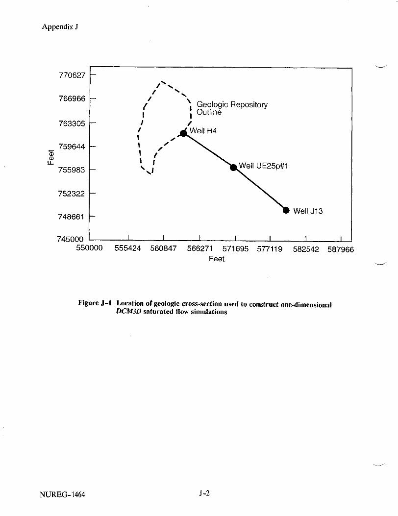
Appendix J
555424 560847 566271 571695 Feet
577119 582542 587966
Figure J-I Location of geologic cross-section used to construct one-dimensional DCM3D saturated flow simulations
NUREG-1464
770627
766966
763305
759644
755983
752322
748661
IL
It
/ Geologic Repository I IOutline I I
/ WellIH4 - ! /
~ I Well UE25p#1
Well J13
II I I I I745000 1
550(000
J-2

Appendix J
1200 WELL
A H-4 1100- 0 UE25p#1
S[0 J-13
1000
S900 S~Tsw "
c800 0 "• CHnz _WATER TABLE ,_
700
600 -
500 PPw
400 . . . . I
0 1000 2000 3000 4000 5000 6000
ZL 0Horizontal Distance (meters)
x
Figure J-2 Geologic cross-section based on Wells H1-4, UE25p#1, and J-13
NUREG-1464J-3

Appendix J
Table J-1 Input Data for DCM3D One-Dimensional Simulations
Topopah Spring
Description
Average matrix Maximum matrix Minimum fracture Maximum fracture From well tests
Ksat (m/yr)
6.0 x 10⁻⁴
6.0 x 10⁻²
3.0 x 10⁻⁴
3.0 x 100 2.8 x 10²
Calico Hills
Porosity
0.11
0.11
0.000021
0.000041
0.000041
Ksat (m/yr)
6.0 x 10⁻⁴
6.0 x 10⁻²
3.0 x 10⁻³
3.0 x 100 2.0 x 101
porosity values as Run Nos. 3 and 4 were used in Run No. 5.
Each simulation was run until it approached steady-state conditions. Table J-2 contains output from these runs. Output is presented in the form of average Darcy velocity, average seepage velocity, and flow time from one end of the simulation to the other (calculated from the seepage velocities).
J-3 SUMMARY OBSERVATIONS/ CONCLUSIONS FROM RUNS
A number of interesting observations can be made from these runs:
(1) The slowest velocities and longest flow times were obtained from runs that used matrix properties. Seepage velocities were 1.3 x 10⁻⁶ and 1.6 x 10⁻⁵ meters/year, resulting in extremely long calculated flow times of 3180 million years and 31.7 million years. This indicates that in this model, matrix flow cannot readily transport radionuclides from the site.
(2) The fastest velocities and shortest flow times were obtained from runs that used hydrologic properties from well tests. The average seepage velocity was 473 meters/year and the calculated flow time was 10.6 years.
(3) Run No. 3 was constructed using minimum fracture flow properties with saturated hydraulic conductivities as low as the matrix
property runs (Run Nos. 1 and 2). However, Run No. 3 produced faster flow velocities and shorter flow times than the matrix property runs, because of the small porosity values used in the Run No. 3 simulation. Since porosity values used in all the fracture property runs were hypothetically determined, they illustrate the importance of porosity in flow velocity calculations and the need to determine representative bulk fracture porosities during site characterization.
A plot of hydraulic heads for each of the runs was prepared to compare the results from each simulation to the cross-section water levels (see Figure J-3). The cross-section water table illustrates the low head gradient over this distance (2 meters). A change in the head gradient occurs at 2310 meters, which is where the hydrogeologic stratigraphy in the cross-section changes from the Calico Hills unit to the Topopah Spring unit. Run No. 3, using minimum bulk fracture values, produced the best match in heads. The staff recognizes that a match between predicted and actual heads does not prove that a model is correct. However, it does provide added confidence that the range of iterative performance assessment hydraulic conductivity values may be conservative (produce fast flow rates).
J-4 REFERENCES Ababou, A.C., 'Approaches to Large Scale Unsaturated Flow in Heterogenous, Stratified, and Fractured Geologic Media," U.S. Nuclear Regulatory Commission, NUREG/CR-5743,
NUREG-1464
Run No.
1 2 3 4
5
Porosity
0.28 0.28
0.000046
0.000046 0.000046
0.000046
Calico Hills
J-4
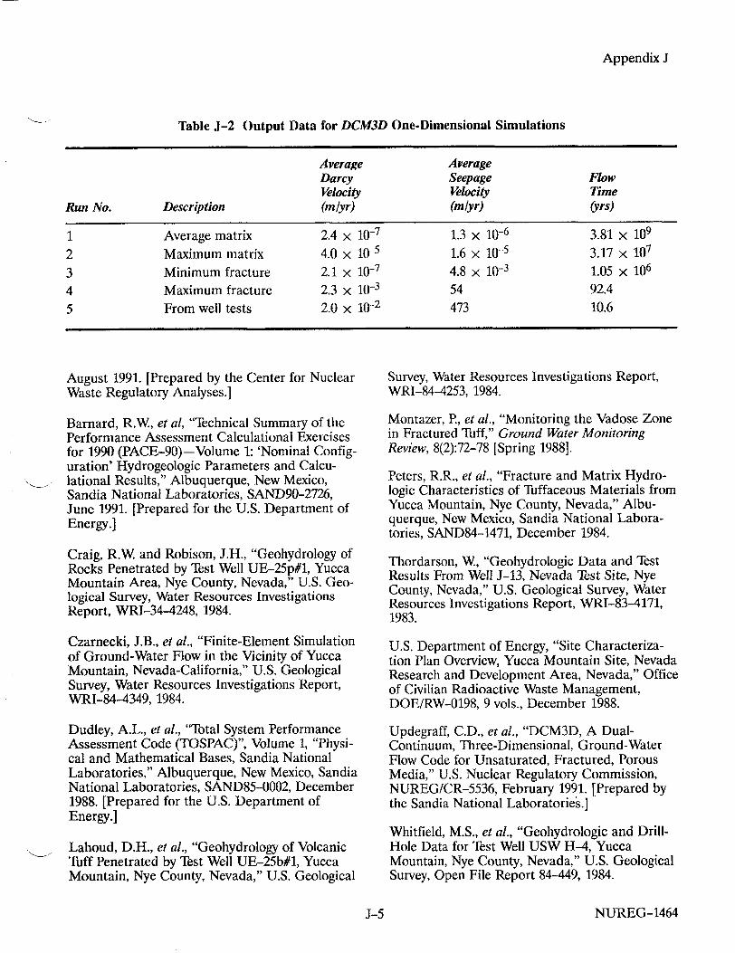
Appendix J
Table J-2 Output Data for DCM3D One-Dimensional Simulations
Average Average Darcy Seepage Flow Velocity Velocity Time
Run No. Description (mlyr) (m/yr) (yrs)
1 Average matrix 2.4 x 10⁻⁷ 1.3 x 10⁻⁶ 3.81 x 10⁹ 2 Maximum matrix 4.0 x 10-S 1.6 x 10⁻⁵ 3.17 x 10⁷
3 Minimum fracture 2.1 x 10⁻⁷ 4.8 x 10- 3 1.05 X 10⁶
4 Maximum fracture 2.3 x 10⁻³ 54 92.4 5 From well tests 2.0 x 10⁻² 473 10.6
August 1991. [Prepared by the Center for Nuclear Waste Regulatory Analyses.]
Barnard, R.W, et al, "Technical Summary of the Performance Assessment Calculational Exercises for 1990 (PACE-90)-Volume 1: 'Nominal Configuration' Hydrogeologic Parameters and Calculational Results," Albuquerque, New Mexico, Sandia National Laboratories, SAND90-2726, June 1991. [Prepared for the U.S. Department of Energy.]
Craig, R.W. and Robison, J.H., "Geohydrology of Rocks Penetrated by Test Well UE-25p#1, Yucca Mountain Area, Nye County, Nevada," U.S. Geological Survey, Water Resources Investigations Report, WRI-34-4248, 1984.
Czarnecki, J.B., et al., "Finite-Element Simulation of Ground-Water Flow in the Vicinity of Yucca Mountain, Nevada-California," U.S. Geological Survey, Water Resources Investigations Report, WRI-84-4349, 1984.
Dudley, A.L., et al., "Total System Performance Assessment Code (TOSPAC)", Volume 1, "Physical and Mathematical Bases, Sandia National Laboratories," Albuquerque, New Mexico, Sandia National Laboratories, SAND85-0002, December 1988. [Prepared for the U.S. Department of Energy.]
Lahoud, D.H., et al., "Geohydrology of Volcanic Tuff Penetrated by Test Well UE-25b#1, Yucca Mountain, Nye County, Nevada," U.S. Geological
Survey, Water Resources Investigations Report, WRI-84-4253, 1984.
Montazer, P., et al., "Monitoring the Vadose Zone in Fractured Tuff," Ground Water Monitoring Review, 8(2):72-78 [Spring 19881.
Peters, R.R., et al., "Fracture and Matrix Hydrologic Characteristics of Tuffaceous Materials from Yucca Mountain, Nye County, Nevada," Albuquerque, New Mexico, Sandia National Laboratories, SAND84-1471, December 1984.
Thordarson, W, "Geohydrologic Data and Test Results From Well J-13, Nevada Test Site, Nye County, Nevada," U.S. Geological Survey, Water Resources Investigations Report, WRI-83-4171, 1983.
U.S. Department of Energy, "Site Characterization Plan Overview, Yucca Mountain Site, Nevada Research and Development Area, Nevada," Office of Civilian Radioactive Waste Management, DOE/RW-0198, 9 vols., December 1988.
Updegraff, C.D., et al., "DCM3D, A DualContinuum, Three-Dimensional, Ground-Water Flow Code for Unsaturated, Fractured, Porous Media," U.S. Nuclear Regulatory Commission, NUREG/CR-5536, February 1991. [Prepared by the Sandia National Laboratories.]
Whitfield, M.S., et al., "Geohydrologic and DrillHole Data for Test Well USW H-4, Yucca Mountain, Nye County, Nevada," U.S. Geological Survey, Open File Report 84-449, 1984.
NUREG-1464

Appendix J
730.5
730.0 / WaterTable S",•, Run 3
a)
r-: 72. ,Rn 0)
CZ
.o * 44
> %%
-. 729.0 w •
............. ........... ... 72 . 1 1*1 ........."o 728.0
" 0 1000 2000 3000 4000 5000 6000
Horizontal Distance (Meters)
Figure J-3 Plot of water table and computer run head elevations
NUREG-1464 J-6

APPENDIX K GEOCHEMICAL MODEL FOR 14C TRANSPORT IN UNSATURATED ROCK
K-I INTRODUCTION
Under oxidizing conditions in a geologic repository, 14C in high-level radioactive waste might be
released as 14C0 2 (Light et al., 1990). Any such gas escaping the engineered barrier will be incorporated in the existing carbon system of the geosphere, and be transported along with gaseous and dissolved carbon. Several recent studies addressed 14C gaseous transport at the Yucca Mountain repository environment using simplified models of geochemical retardation (Ampter and Ross, 1990; Light et al., 1990; and Knapp, 1990). Accurate modeling of 14C transport requires coupling of relations between the source, heat flow, two-phase fluid flow, and the distribution of
chemical species among solid (s), liquid (1), and gas (g) phases (Codell and Murphy, 1992). Interphase exchange of carbon could result in a significant retardation of released 14 C, thereby delaying its arrival at the accessible environment. This auxiliary analysis reports on a mechanistic model for the geochemical interaction of 14C for a geologic repository in partially saturated rock.
The 14 C transport model consists of three parts:
(1) A geochemical model describing the state of all carbon species in a representative volume of rock;
(2) A flow and transport model for movement of
total carbon through the system which consists of a number of connected volumes or "cells"; and
(3) A model of 14C migration as a trace quantity in the general movement of total carbon.
K-2 GEOCHEMICAL MODEL
A carbon system geochemical model which incorporates all reactions of primary significance
to 14C transport in unsaturated fractured rock can
be based on local chemical equilibrium and mass
and charge conservation in a representative volume. Chemical reactions in the model comprise carbonate equilibria among aqueous (aq)
species, dissociation of water, vapor-liquid equilibria for CO 2 and H20, and calcite dissolution and precipitation. In addition to the aqueous species in these equilibria, the present model includes Na+ to represent other aqueous cations. The reactions represented in the present model are given next:
H20(l) + C0 2(aq) U5 H+ + HC03
HCO3 U H+ 3HCO
H+ + OH- U H20
(K-1)
(K-2)
(K-3)
(K-4)
(K-5)
CaC0 3(s) + H+ U5 Ca 2+ + HCO3
C0 2(g) = C0 2(aq)
Local charge balance in the model aqueous phase is represented by equating sums of aqueous cation and anion equivalents. Local mass conservations for carbon and calcium are maintained within each cell, and the mass of sodium is conserved in the aqueous phase.
Given the total masses of C, Ca and other species, mass of water, and the temperature, pore volume and pressure of each cell, the above relationships lead to a set of nonlinear algebraic equations that are solved simultaneously to characterize local equilibrium in each cell for each time step. Equilibrium constants for reactions 1 to 5 are functions of temperature only at one bar pressure. Activity coefficients are functions of ionic strength, and are generated from an extended Debye-Lihckel equation. Calcite is permitted to precipitate or dissolve at equilibrium, and the model solution is undersaturated with respect to calcite in its absence. The partial pressure of CO 2
is calculated from the activity of aqueous C0 2, assuming ideal gas relations.
NUREG-1464K-1
Appendix K
K-3 TOTAL CARBON TRANSPORT MODEL
The calculation of transport of total carbon through the modeled system is performed by sequential iteration in the following steps:
(1) Local chemical equilibrium is calculated in each cell at time t, using the geochemical model;
(2) Inputs and outputs to each cell are determined from an independent flow model for the next time step t + At. In the present model, only advective transport by gaseous flow is allowed. Therefore, the input of CO2 to a cell is determined only by the partial pressure of CO 2 in the previous cell or upstream boundary and the flow of the transporting gas from that cell. Gaseous flow and condensation/evaporation of water are accounted for independently as part of the flow model and input to the chemical model; and
(3) Mass distributions are revised in the cells for time step t + At, using the geochemical model with updated temperature and liquid saturation states.
The carbon transport algorithm in the preceding steps simulates changes to the chemistry of each phase in the system, as a function of time and space. The carbon transport model determines the quantities of CO2 gas moving through the system of cells, as well as the exchange rates of carbon between the various phases.
K-4 14C TRANSPORT MODEL The 14C transport model uses the state and evolution of total carbon speciation to simulate transport of trace amounts of 14C through the system.
C is assumed to behave exactly in proportion to the total carbon, with no isotopic fractionation. However, radioactive decay removes 14C from the solid, liquid, and gas inventories. The model assumes 14C enters the system as an instantaneous pulse within a specified cell. 14C is removed from the liquid/gas phases if calcite precipitates from solution. It re-enters the system if previously contaminated calcite dissolves. The model assumes that calcite dissolves first from the
14C-contaminated calcite inventory before uncontaminated calcite redissolves. The model further assumes that the 14C is distributed homogeneously within the contaminated calcite of each cell.
K-5 EXAMPLE
The present geochemical transport model has been applied to simplified examples, to demonstrate the range of possible phenomena associated with the release and transport of 14C0 2 in unsaturated fractured rock. The model system is a one-dimensional column of 145 cells, represented in Figure K-i, with constant hydraulic properties and cross section, passing through the center of a hypothetical repository plane, which is located at cell 55. Water, gas, and relevant mineral chemistries, as well as the geothermal gradient that resemble those factors observed at Yucca Mountain, are provided as initial conditions. The system chosen for the example was simple, so as not to confound the results of the geochemical transport model with other phenomena. For example, gas is assumed to flow in the upward direction only, even though thermal-hydraulic simulations indicate an initially outward gas flow in all directions from a heated repository in unsaturated tuff (Nitao, 1990). Additionally, there is no transport of 14C by water flow or diffusion in gas or water.
Time-dependent temperature and gas flow used in the present example were generated from twodimensional (2-D) codes, developed by the U.S. Nuclear Regulatory Commission staff for predicting air flow through Yucca Mountain. The NRC models are similar to those developed by Ampter and Ross (1990). Temperature, represented in Figure K-2, was calculated from a 2-D thermal conduction model that included the geothermal gradient. Gas flux, shown in Figure K-3, varied with time, but was uniform through the one-d imensional column.
Liquid saturation is shown in Figure K-4. The temperature and gas flow models did not include water saturation explicitly. Therefore, an approximate empirical model for saturation of the column was derived from the results of simulations of two-phase thermally induced circulation near repositories in tuff. The empirical model
NUREG-1464 K-2

Appendix K
Depth Below
Surface 0.0 m
450 m
725 m - L
Volume Position
- 145
- 55
- 1 -
A4
• - Constant Temperature Boundary
- Local Chemical Equilibrium in each Representative Volume
Uniform Gas Flow in one Dimension
*-Repository:
Heat Source and 14 C Source
*-Gas Input with CO2
Figure K-1 One-dimensional flow and transport model
NUREG-1464K-3

Appendix K
150
140
130
120 0- 1years
-- 100 110 ON 1 O •,•.--"-- 1000
-2000 100- -\\ --- 4000
90 - ... •. .0. *
90 :- 0 . 6o "
50 - .•.•.2..
40 -,
30 -- "':
'0,P 20 - ,
40 30- - - I
,"F,
0 II
280 300 320 340 360 380
Temperature (OK)
Figure K-2 Temperature in one-dimensional model as a function of time
NUREG-1464 K-4
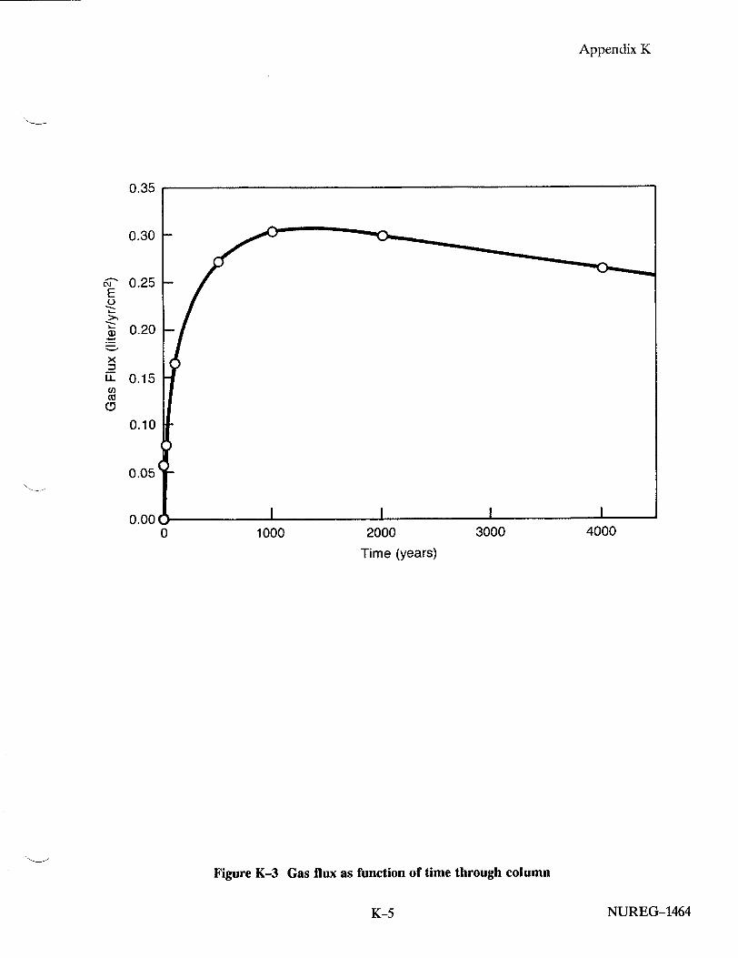
Appendix K
2000
Time (years)
Figure K-3 Gas flux as function of time through column
K-5 NUREG-1464
C\j E
(.)
ci,
.0
0.35
0.30
0.25
0.20
0.15
0.10
0.05
0.00
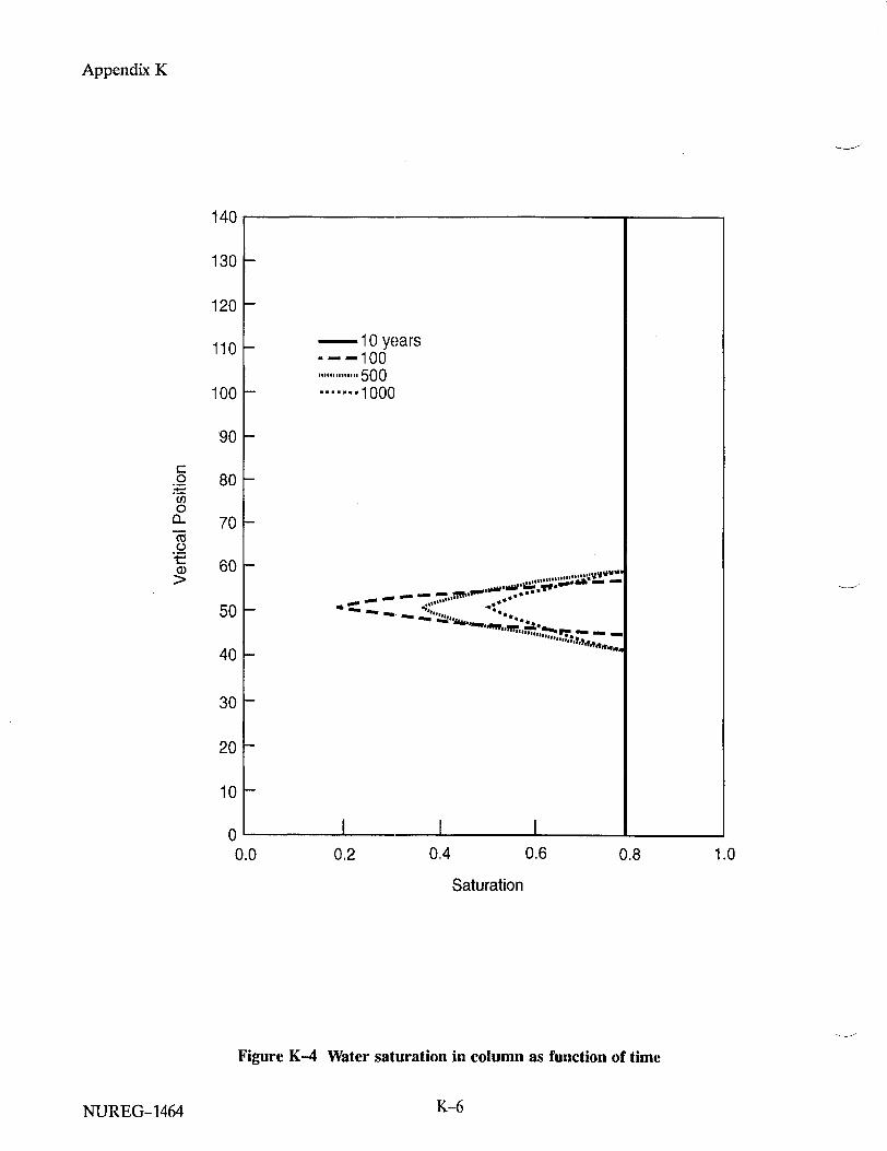
Appendix K
140
130
120
110 - 10 years --- 100 11 ....I........ 500
100 ....... 1000
90
.o 80
0 IL 70
1= 60
50 "- - - .... "'"1 ,m.wwYw&
40
30
20
10
0 I I I
0.0 0.2 0.4 0.6 0.8 1.0
Saturation
Figure K-4 Water saturation in column as function of time
NUREG-1464 K-6

Appendix K
used in the example predicts that water saturation is 80 percent except within a zone of about 50 meters above and below the repository for a period of less than 2000 years.
Other initial conditions and parameters of the example system are given in the Table K-1. These conditions lead to an initial solution with pH 7.2, moderately undersaturated with respect to calcite with the QIK (saturation index/equilibrium constant) about 0.2, and partial pressures of CO 2 in the range 0.005 to 0.008 bar, depending on temperature.
Results for the Carbon Model: Results for the carbon transport model are given in Figure K-5, which shows the distribution of carbon for each cell among the gas, liquid, and solid phases for various times after repository closure. Initially, the carbon content decreases in the liquid phase and increases in the solid and gas phases near the repository level. Just above the repository, however, the carbon content of the gas and liquid phases increases, a reflection of gas transport of the pulse of CO2 initially volatilized from the liquid near the repository and transported. Increasing temperature, decreasing solvent mass, and increasing pH because of CO2 volatilization all promote calcite precipitation near the repository horizon.
At 500 years, the initially volatilized CO 2 pulse has been flushed out the top of the column. The calcite content continues to grow, spreading above and below the repository level, as temperature increases. At 2000 and 4000 years, the calcite progressively redissolves while the liquid content of carbon increases as the rock cools.
Results of 14C Model: Figure K-6 shows the distribution of 14C for each cell in the gas, liquid and solid phases, at various times for 10-6 curies of 14C released 15 meters below the assumed repository plane at time zero. The 14C was released below the repository plane to account for gas circulation expected near the repository, and allows interaction of the contaminant below as well as above the engineered barrier.
At 100 years, most of the 14C has redistributed to the liquid phase. The liquid and gas inventories of 14C have moved above the repository plane be
cause of gas transport, even though the fraction of 14C in the gas phase is small. The 14C in the calcite remains fixed until calcite redissolves. At 500 years, the gas and liquid inventories of 14C have moved further above the repository plane. Some of the calcite near the repository plane redissolves, releasing its 14C inventory, which in turn is partially captured by precipitating calcite further from the repository plane, where temperature continues to increase.
Table K-I Initial Conditions and Parameters
Parameter Value
Cell Cross Section
Cell Spacing
Cell Volume
Porosity
Initial Saturation
Initial C/cell
Na/cell
Ca/cell
CO 2 Input Gas
12.5 cm 2
5m
6250 cm 3
0.2
0.8
0.00202 moles
0.001 moles
0.0004 moles
2.53 x 10- 4 moles/liter
NUREG-1464K-7
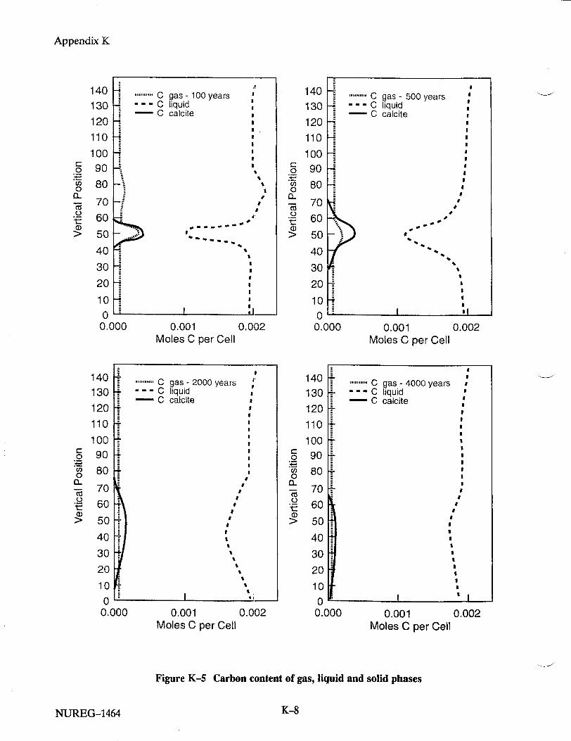
Appendix K
0
0 0o
76
0)
0
0
C-)
._o
140
130
120
110
100
90
80
70
60
50
40
30
20
10 0
0.0
140 130
120
110
100 90
80
70 60
50
40
30
20
10
0 0.0
S ..... C gas -l100years
"---C Liquida - C calcite
II
I II I |
I I
II
*
-z I
II
4 '
iI
0.001 0.002 Moles C per Cell
0
.2 0
a_
0.001 0.002 Moles C per Cell
0 (0
0
CL)
140
130
120
110
100
90
80
70 60
50
40
30 20
10 0 0.000
140 130
120
110
100 9o 80
70
60
50
40
30
20 10 0 0.000 0.001 0.002
Moles C per Cell
Figure K-5 Carbon content of gas, liquid and solid phases
NUREG-1464
0.001 0.002 Moles C per Cell
00
00
K-8
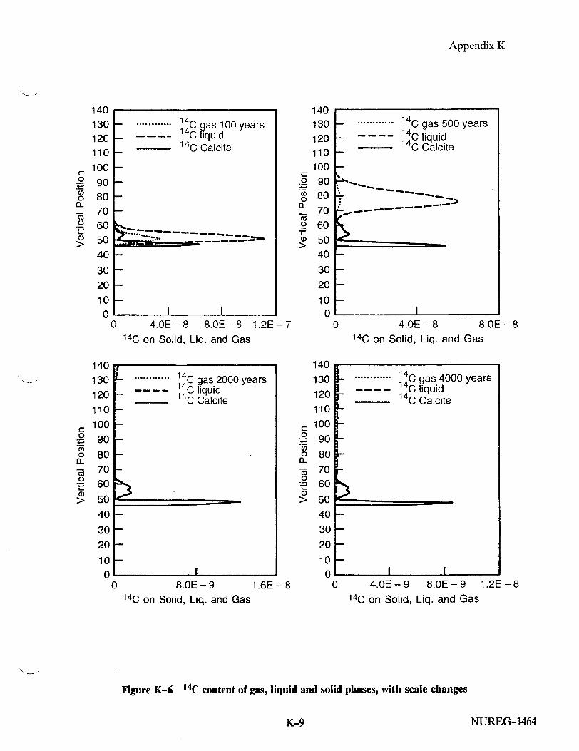
Appendix K
140 130 120 110
100
90 80 70 60 50 40
30 20
10 0
140 130
120
110
100
90
80 70
60
50
40
30
20
10 0
0 4.OE-8 8.OE-8 1.2E-7 14C on Solid, Liq. and Gas
r0
0 D.
I.
C: 0 pl, 0
a.)
8.E - 9 1.6E - 8 14C on Solid, Liq. and Gas
S............ 14C gas 100 years 14 C liquid 14C Calcite
140 130
120 110 100
90 80 70 60
50 40
30 20
10 0
140
130
120
110
100
90
80 70
60
50 40
30
20
10 0
4.OE - 8 8.OE - 8 140 on Solid, Liq. and Gas
0 4.OE - 9 8.OE - 9 1.2E - 8 14C on Solid, Liq. and Gas
Figure K-6 1 4 C content of gas, liquid and solid phases, with scale changes
NUREG-1464
0
. ............ 140 gas 500 years 140 liquid
- 14C Calcite
- --
0
a_
"-FO
C:
0 03
0o
C.
I. 0as 2000 years
14C liquid 14C Calcite
0
K-9
Appendix K
By 2000 years, nearly all 14C is swept from the column, except that which remains trapped in the calcite. At this point in time, calcite is redissolving everywhere, so the contaminated calcite acts as a long-term source of 14C to the system. Some of this residual 14 C remains even at 4000 years.
Dependence on Time of Release: The model predicts that calcite starts to precipitate shortly after repository closure and then redissolves. Therefore, the timing of the release of 14C from the waste is important to its ultimate fate. 14C released after most calcite has precipitated will not be removed from the liquid and gas phases as effectively as 14 C released during the period of active calcite precipitation. Figure K-7 shows the cumulative release, over 1500 years after repository closure, of 14 C past several points in the column as a function of time of 14C release. This figure demonstrates the interesting phenomenon that 14C released at early times can arrive at the end of the column after 14 C released at later times.
K-6 CONCLUSIONS
Numerical experiments with a flow and transport model that includes coupled nonisothermal geochemistry provide insights into the behavior of 14 C in an unsaturated geologic repository for nuclear waste. These experiments have been applied to a system resembling the proposed repository at Yucca Mountain, Nevada. Model results show a significant redistribution of autochthonous carbon among solid, liquid, and gas phases, even in areas remote from the repository plane. Carbon remains predominantly in the aqueous solution, in spite of the fact that nearfield heating results in a reduction of liquid saturation, abundant calcite precipitation, and increased equilibrium fractionation of CO 2 into the gas phase.
Transport of 14C released from the repository is generally retarded by a factor of approximately 30 to 40, because of immobilization in the liquid phase. In addition, 14C released early during the period of solid calcite precipitation can be fixed for a long period before repository cooling leads to redissolution of the calcite.
Although simplified, the model demonstrates the complex nature of the geochemical processes affecting 14C release. Results of the simulation depend strongly on model assumptions, and retardation of 14C in the liquid or solid phases could be greater or smaller under different conditions of chemistry, hydrology, temperature, or gas flow. The staff contemplate coupling geochemistry and carbon transport models with more realistic two-or-three-dimensional treatments of heat and mass transfer near a repository in unsaturated tuff, which would include transport in the gas and liquid phases and allow for molecular diffusion.
K-7 REFERENCES
Amter, S. and B. Ross, "Simulation of Gas Flow Beneath Yucca Mountain, Nevada, with a Model Based on Fresh Water Head," in Post, R.G. (ed.), Waste Management '90: Proceedings of the Symposium on Waste Management, February 25 March 1, 1990, Tucson, Arizona, 2:915-925 [1990].
Codell, R.B. and WM. Murphy, "Geochemical Model for 14 C Transport in Unsaturated Rock," American Nuclear Society/American Society of Civil Engineers, Proceedings of the Third International Conference.- High-Level Radioactive Waste Management, April 12-16, 1992, Las Vegas, Nevada, 2:1959-1965 [1992].
Knapp, R.B., 'An Approximate Calculation of Advective Gas-Phase Transport of 14C at Yucca Mountain, Nevada", Journal of Contaminant Hydrology, 5:133-154 [1990].
Light, WB., et al., 'Analytical Models for C-14 Transport in a Partially Saturated, Fractured, Porous Media," American Nuclear Society, Proceedings of the Topical Meeting on Nuclear Waste Isolation in the Unsaturated Zone (FOCUS '89), September 17-21, 1989, Las Vegas, Nevada, pp. 271-277 (1990].
Nitao, J.J., "Numerical Modeling of the Thermal and Hydrological Environment Around a Nuclear Waste Package Using the Equivalent Continuum Approximation: Horizontal Emplacement," Livermore, California, Lawrence Livermore National Laboratory, UCID-21444, May 1990.
K-10NUREG-1464

Appendix K
1.00
0.95
I 0.90 ci) (D I)
=3 0.85 E =3
0.80
0.75
0.70 L0.0 200.0 400.0 600.0 800.0 1000.0
Time of Release (years)
Figure K-7 Cumulative release by 1500 years as a function of when 14 C was released
NUREG-1464K-11

APPENDIX L THE EXCHANGE OF MAJOR CATIONS AT YUCCA MOUNTAIN
L-1 INTRODUCTION
An important characteristic of Yucca Mountain, the proposed geologic repository for high-level radioactive waste (HLW), is the presence of zeolitic tuffs. Zeolites are crystalline, hydrated aluminosilicates, which are characterized by an ability to readily exchange cations with aqueous solutions. The presence of zeolites is seen as an important barrier to the migration of radionuclides to the accessible environment. This auxiliary analysis was designed to answer two questions related to the exchange of cations in Yucca Mountain.
The first question concerned the stability (i.e., constancy of exchangeable cation composition) of zeolites. Using potassium/argon (K/Ar) dating techniques, WoldeGabriel et al. (1992) determined that the zeolites from drillholes in the Yucca Mountain vicinity range in age from 2 million years to 10 million years old. However, ion exchange involving potassium and sodium on zeolites has been shown to reach equilibrium in about 2 days (Pabalan, 1991). How, then, can a mineral that can alter within a couple of days exist for at least 2 million years? To answer that question, simulations were performed in which pore water, whose composition approximates that found at Yucca Mountain, percolates through site-specific zeolite layers for a period of approximately 150,000 years. The simulation was intended to represent the chemical reactions that would take place between the cations dissolved in the pore water and the cations sorbed onto zeolites. If, in the simulation, the K ions attached to the zeolites become mobile, there would be reason to doubt the zeolites could be accurately dated, using a K/Ar technique. If, however, the K is immobile, the K/Ar ratios would not be affected by ion-exchange reactions. This information is important to the siting of the repository, for it supports the conceptualization that the zeolites should remain stable for the lifetime of the repository and should act as a barrier for the release of radionuclides to the accessible environment (10 CFR 60.2).
The second question to be answered by this analysis involved the determination of pore water compositions from the unsaturated zone. Peters el al. (1992) describe methods of measuring pore water compositions from rocks of the unsaturated zone, plus the possible causes of changes in the compositions of the pore waters because of the method of extraction (compression). Given that ion-exchange reactions involving zeolites are fast (Pabalan, 1991), can we determine the chemical composition of pore water from the unsaturated zone, if the composition of the zeolite in direct contact with the pore water is known? If the answer is yes, then are there any significant spatial patterns of these compositions?
L-2 BACKGROUND Ion exchange is a process by which ions in one phase displace ions in another phase. For example:
m A" + nBX,, = m AX,, + nB"+ (, (L-
where A and B represent cations of charge n and m, respectively, and X represents the sorption site on the solid phase. The cation exchange capacity (CEC) and the quantity of major cations present in a system can strongly influence the exchange or distribution coefficient (Kd) of radionuclides, as shown in the following equations:
Rn +NaX =RnX + Na ,
K - [RnX][Nal [Rn][NaX]
[Na]
(L--2)
(L-3)
(L-4)
where Rn represents a radionuclide, Kd is the distribution of the radionuclide between the solid and the aqueous phase, K is the equilibrium constant, and brackets represent activities. The Kd of a specific nuclide in a specific environment is commonly used when describing sorptive properties. Since Kd is directly related to the cation content, an understanding of the major
NUREG-1464L-1

Appendix L
cation chemistry (Na+, Ca2 +, and K+) is needed to fully understand the ability of Yucca Mountain to sorb radionuclides.
L-3 GEOCHEMICAL CODE The simulations performed to address the first question in this auxiliary analysis concerning the validity of K/Ar dating relied on the geochemical modeling code PHREEQM, a code for use in mixing cell flowtube simulations, described by Appelo and Willemsen (1987). PHREEQM (Ph-REdox-EQuilibrium-Mixing), a modification of PHREEQE, has the same capabilities of PHREEQE, plus it can simulate one-dimensional fluid flow, diffusion, dispersion, and ion exchange. PHREEQE (Ph-REdox-EQuilibrium-Equations) is based on an ion-pairing aqueous model and can calculate pH, redox potential, and mass transfer as a function of reaction progress (Parkhurst et al., 1980).
PHREEQM has the ability to simulate the flow of a solution through a multilayered heterogeneous column of porous material. Up to 10 layers, or a total of 100 cells, can be included in the simulated column. In each layer, equilibration with up to 10 minerals and reaction with up to 10 components can be simulated. Initial solid and liquid compositions in the column are input parameters of the code. Other input parameters are the length of each cell, the dispersivity associated with each cell, the porosity of any cell, the number of cell volumes of flushing solution added to the column, the composition of the flushing solution, the time allowed for diffusion/mixing of chemical constituents between adjacent cells, and the molecular diffusivity of elements in water.
Output includes composition of liquid, quantities of minerals precipitated or dissolved, and composition of solid ion exchanger in each cell for all time-steps. The output is presented in spreadsheet format, to facilitate the graphing of the results.
L-4 SIMULATIONS
L-4.1 Effect of Ion Exchange on K/Ar Dating
This analysis involved simulating the flow of site-specific ground water, through site-specific porous rock, at a site-specific rate. The simulation that was performed used mole fractions of Na,
Ca + Mg, and K derived from the zeolite compositions reported by Broxton et al. (1986). In that study, the mole fractions of the exchangeable cations were determined for an extensive array of samples taken from boreholes in the vicinity of Yucca Mountain, in both the saturated and unsaturated zones. The zeolitic compositions vary both laterally and vertically. To simplify the simulation, a solid ion-exchanger composition was chosen that approximates the average composition of zeolites from the Topopah Spring member of the Paintbrush Tuff, where the proposed HLW repository is to be sited. The relative mole fractions for Ca + Mg, Na, and K were 33 percent, 19 percent, and 48 percent, respectively. The flushing solution composition in the simulation approximates that of the site-specific water from Peters et al. (1992). This site-specific water was extracted from pores, from several representative samples of tuff, by means of compression. Given that the zeolite compositions from Broxton et al. summed the concentrations of the exchangeable cations, Ca and Mg, the same was done for the liquid. The composition of the simulated water (flushing solution) was 3.10 moles/liter Ca + Mg, 1.83 moles/liter Na, and 8.03 moles/liter Cl. Other chemical constituents measured in the pore water from the squeezed rock but not included in this simulation, were H, HCO3, S04, and SiO 2. These constituents have no effect on the reaction modeled.
The column through which water flowed in the simulation was divided into 100 cells. Each cell was 5 meters long. The whole column was then composed of 500 meters of the Paintbrush Tuff unit. The porosity of the column is assumed to be 0.3, which lies within the range of porosities found at Yucca Mountain.
The percolation flux of flushing solution through the column was set at 0.6 millimeters/year. This is comparable to moving the liquid from one cell to an adjacent cell downstream every 2500 years. This value approximates that derived from matrix potentials in Well USW UZ-1 (Montazer et al., 1986). The range of estimates of percolation fluxes, however, extend from negative values (upward fluxes) to 100 millimeters/year (Montazer and Wilson, 1984; and Montazer et al., 1986). The dispersivity associated with each cell was arbitrarily set at 0.02 meters. Molecular diffusivity was 3 square meters/100 years.
NUREG-1464 L-2

Appendix L
The CEC was set at 6667 milliequivalents/liter. This value lies approximately halfway between the extremes of CEC's of rocks from Yucca Mountain (from Thomas, 1987). The three ion-exchange reactions modeled are:
NaX + K+ KX + Na+ ,
2Na+ + CaX2 i 2NaX + Ca2+
2K+ + CaX2 ± 2KX + Ca2+
(L-5)
(L-6)
(L-7)
Equilibrium constants for Equations (L-5) and (L-6) were from Pabalan (1991). The equilibrium constant for Equation (L-7) was derived by multiplying Equation (L-5) by two and adding the result to Equation (L-6). In this simulation, ideal mixing was assumed in the solid phase. This assumption is most likely incorrect, as indicated by the experimental evidence of nonideality in the binary systems Na-K and Na-Ca clinoptilolite (Pabalan, 1991). However, experimental studies on mixing in the solid phase of the ternary system Na-K-Ca clinoptilolite have yet to be performed, so the assumption of ideality in the solid phase was required.
L-4.2 Calculated Compositions of Water from the Unsaturated Zone
By using the compositions of clinoptilolites from the unsaturated zone of Yucca Mountain (from Broxton et al., 1986) and the equilibrium constants from Pabalan (1991) and this study for Equations (L-5) through (L-7), the relative concentrations of the exchangeable cations in the pore were calculated. Again, ideality of mixing in the solid was assumed. Activity coefficients for species in the liquid phase were derived from the Debye-Hliickel formulation. However, the ionic strength of pore water in equilibrium with the zeolites is assumed to be constant and comparable to the extracted pore water from Peters et al. (1992). Consequently, the activity coefficients are likewise constant.
L-5 RESULTS
L-5.1 Effect of Ion Exchange on K/Ar Dating
Figure L-1 shows the concentration of exchangeable cations in the solid versus distance along flow path (represented as cell numbers). Cell 0
represents the top of the column; cell 100 represents the bottom of the column. The flushing solution is input into the top of the column at cell 0. The horizontal lines represent the chemical composition of the solid phase in the column after 60 shifts (cell volumes) or 150,000 years. The composition is relatively constant, except in the first few cells.
Figure L-2 represents the composition of the solution passing through the column after 60 shifts. The original water composition is shown on the Y-axis. This graph demonstrates that the composition of the pore water is dominated by the composition of the zeolites. Since the composition of the zeolites varies, it is reasonable to assume that the pore water chemistry will also vary, as the water percolates through the zeolites.
The results of this auxiliary analysis demonstrate that the K in the zeolites is relatively immobile. This is because of the large reservoir of K held in the zeolite versus the amount of exchangeable cations in the liquid. There simply are not enough cations in the pore water to exchange with the K on the zeolites, and therefore the K remains immobile. Consequently, the K/Ar technique for determining the age of the zeolites should not be affected by ion exchange, given the low concentrations of cations in the ground water.
L-5.2 Calculated Compositions of Water from the Unsaturated Zone
The compositions of zeolites and ground waters in equilibrium with those zeolites were plotted on ternary diagrams using the code GRAPHER. The ternary diagrams illustrate the relative concentrations of sodium, potassium, and calcium and not the total concentrations. This representation for the liquid compositions is consistent with ternary representations of solid compositions in Broxton et al. (1986). Figure L-3 is a ternary diagram showing the relationship of the zeolite compositions to the liquid compositions, in equilibrium with those solids in Well G-4. This figure contains solid and liquid compositions from the unsaturated zone. The solid compositions have an average K content of 50 percent. However, the water in equilibrium with these solids contains very little potassium. The saturated zone information was not included in the graph, so the unsaturated zone information is
NUREG-1464L-3
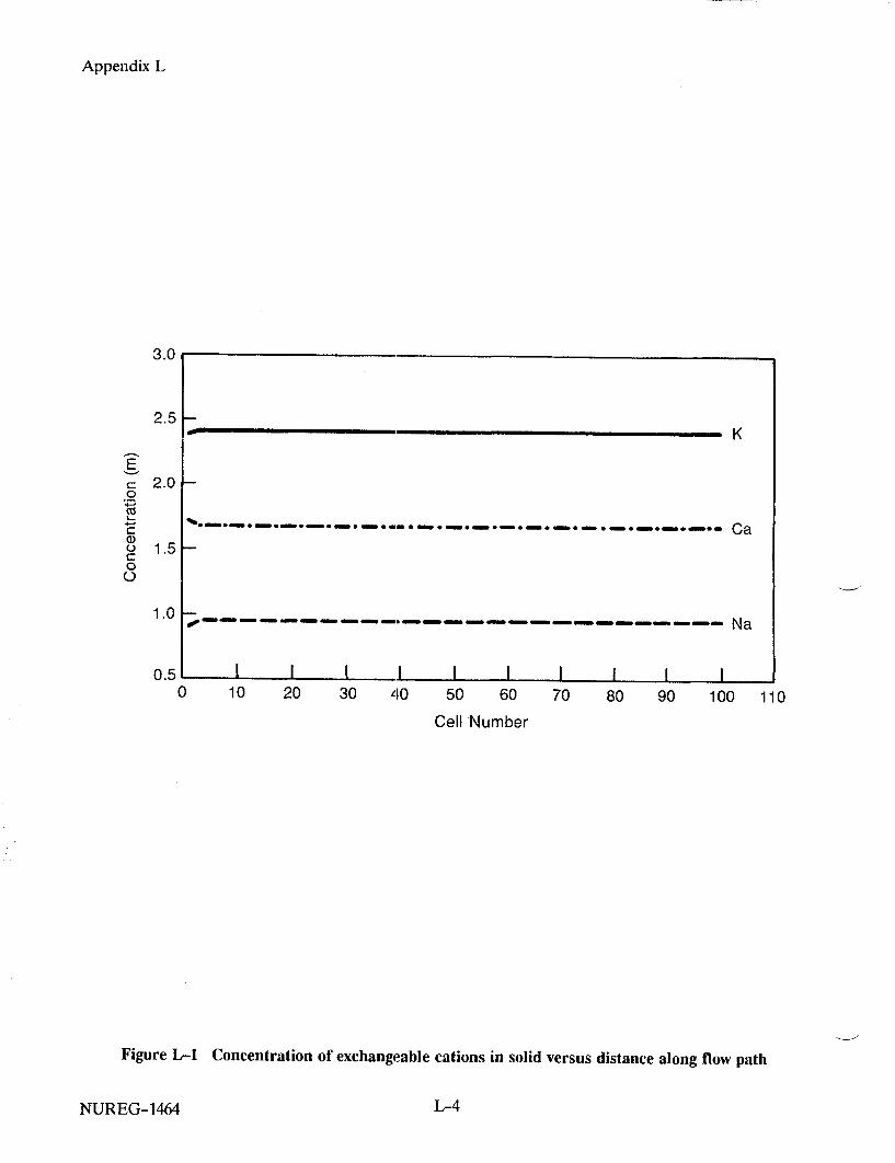
Appendix L
3.0
2.5
E 0 C
.2 0 co
0 0
2.0
1.5
1.0
0.5 L. I I I I I I 0 10 20 30 40 50 60 70 80 90 100 110
Cell Number
Figure L-1 Concentration of exchangeable cations in solid versus distance along flow path
NUREG-1464 L-4
K
S * * ~ -. ~ a.- s~* -en - 0*- -*- *- .a. . a -Ca
- - - - a -- -n. ---- ---- --- -- N a

Appendix L
2.5
2
1.5
0 10 20 30 40 50 Cell
60 Number
70 80 90 100 110
Figure L-2 Composition of solution passing through column
NUREG-1464
4
3.5
Cl)
"0 t-
0
C
0
0 C
--- Na
7
Ca
-K - ---------------- ----- --- -- -
I I I !I I I I II
1
0.5
0
3
L.-5

Appendix L
K
0 0
0= Solid 2-i= Liquid
<0/#
4R
/
Na0 "25 50 75
Figure L-3
NUREG-1464
Ternary diagram of zeolite compositions to liquid compositions in Well G-4 saturated and unsaturated zones using Broxton's solid compositions with liquid in equilibrium
L-6
-o'
0 Ca100

Appendix L
more defined. Figure L-3 clearly demonstrates that the zeolites of the unsaturated zone are deficient in Na, where the pore water in equilibrium is Na-rich and K-deficient. The potassium concentrations of the unsaturated zone pore water measured by Peters et al. (1992) were suspect, and so were not reported. The potassium concentration measured in replicate samples varied, but generally was less than 10 parts per million (C.A. Peters, personal communication, 1993).
Figures L-4 through L-8 illustrate the compositions of zeolites and coexisting ground waters in Wells G-1, G-2, G-3, H-3, and H-4. On Figure L-8, the composition of J-13 well water is plotted, as well as the composition of the water removed from Well USW-H4. The Na-rich composition of the water from USW-H4 is consistent with Na-K-rich zeolites analyzed from this well in the saturated zone. Establishing a comparable match with J-13 ground water/zeolite is not apparent, possibly because of not knowing the depth from which the water comes.
L-6 CONCLUSIONS
In summary, this auxiliary analysis has produced valuable information on the exchange of the major cations in Yucca Mountain. The results indicate that the potassium associated with the zeolites is relatively immobile for the time period of these modeling runs. It also demonstrates the wide variation, in the pore water chemistry, which is possible in this environment. In addition, this analysis has shown that the chemical composition of the pore waters in contact with the solids in the unsaturated zone may be different from the composition of the water in the saturated zone. This is important for those who wish to do exchange experiments and require the solution and solids to be in equilibrium.
L-7 REFERENCES
Appelo, C.A.T and A. Willemsen, "Geochemical Calculations and Observations on Salt Water Intrusions, I., A Combined Geochemical/Mixing Cell Model," Journal of Hydrology, 94:313-330 [1987].
Broxton, D.E., et al., "Chemistry of Diagenetically Altered Tuffs at a Potential Nuclear Waste Repository, Yucca Mountain, Nye County, Nevada,"
Los Alamos, New Mexico, Los Alamos National Laboratory, LA-10802-MS, October 1986.
Montazer, P., and WE Wilson, "Conceptual Hydrologic Model Flow in the Unsaturated Zone, Yucca Mountain, Nevada, Water Resources Investigations," U.S. Geological Survey, Water Resources Investigations Report, WRI-84-4345, 1984.
Montazer, P., et al., "Monitoring the Vadose Zone in Fractured Tuff, Yucca Mountain, Nevada," Proceedings of the National Water Well Association Conference on Characterization and Monitoring of the Vadose (Unsaturated) Zone, Worthington, Ohio, November 19-21, 1985, pp. 439-469 [1986].
Pabalan, R.T, "Nonideality Effects on the Ion Exchange Behavior of the Zeolite Mineral Clinoptilolite," in Abrajano, T, Jr. and L.H. Johnson (eds.), Scientific Basis for Nuclear Waste Management XIV Materials Research Society Symposium Proceedings, 212:559-567 [1991].
Parkhurst, D.L., D.C. Thorstenson, and L.N. Plummer, "PHREEQE-A Computer Program for Geochemical Calculations," U.S. Geological Survey, Water Resources Investigations Report, WRI-80-96, August 1980.
Peters, C.A., et al., 'A Preliminary Study of the Chemistry of Pore Water Extracted from Tuff by One-Dimensional Compression," in Kharaka Y.K., and A.S. Maest (eds.), International WaterRock Interaction Symposium Proceedings, Park City, Utah, July 13-23, 1992, pp. 741-745 [1992]. [Published by A.A. Balkema, Rotterdam, Holland.]
Thomas, K., "Summary of Sorption Measurements Performed with Yucca Mountain, Nevada, Tuff Samples and Water from Well J-13," Los Alamos, New Mexico, Los Alamos National Laboratory, LA-10960-MS, December 1987.
WoldeGabriel, G., et al., "Preliminary Assessment of Clinoptilolite K/Ar Results from Yucca Mountain, Nevada, USA: A Potential High-Level Radioactive Waste Repository Site," in Kharaka, Y.K., and A.S. Maest (eds.), International WaterRock Interaction Symposium Proceedings, Park City, Utah, July 13-23, 1992, pp. 457-461 [1992].
NULJREG-1464L-7

Appendix L
K
0 = Solid [] = Liquid
0
/\/
\a-'---• \ / /
Na. Ca 0 C25 50 75 100
Figure L-4 Ternary diagram of zeolite compositions to liquid compositions for Well G-1 using Broxton's solid compositions with liquid in equilibrium
NUREG-1464 L-8

Appendix L
KQ0
0= Solid [] = Liquid
/4
-- - -- -
-0*
Na I r Ca 0 E25 50 75 100
Figure L-5 Ternary diagram of zeolite compositions to liquid compositions for Well G-2 using Broxton's solid compositions with liquid in equilibrium
NUREG-1464
-A 10"
LI-9

Appendix L
K
0ý
0= Solid 11 = Liquid
cv' 0%
0R IS
Na ( Ca~~ 0 [25 50 75 100
Figure L-6 Ternary diagram of zeolite compositions to liquid compositions for Well G-3 using Broxton's solid compositions with liquid in equilibrium
NUREG-1464 L-10

Appendix L
K
0= Solid E] = Liquid
00
Na" Ca 0 25 50 75 100
Figure L-7 Ternary diagram of zeolite compositions to liquid compositions for Well H-3 using Broxton's solid compositions with liquid in equilibrium
NUREG-1464L-11
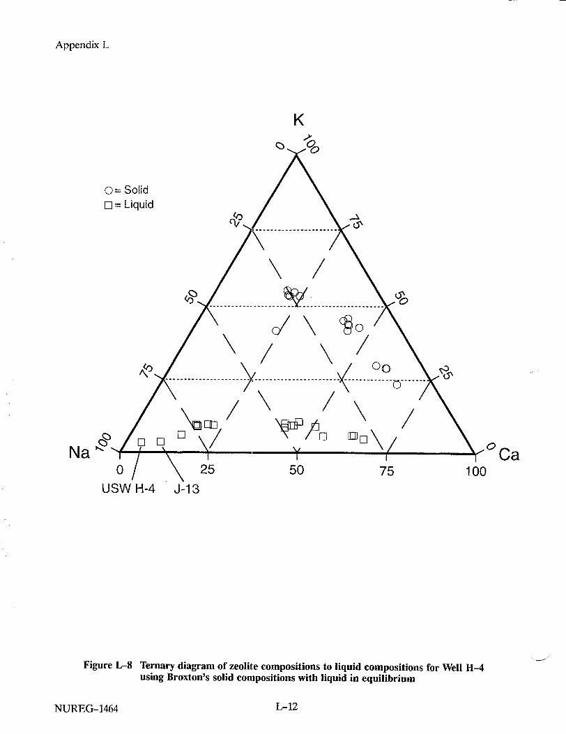
Appendix L
K0I'll
O= Solid Ei = Liquid
S\\N
0 0
25
J-13
0/ USW H-4
Figure L-8 Ternary diagram of zeolite compositions to liquid compositions for Well H-4 using Broxton's solid compositions with liquid in equilibrium
NUREG-1464
A..
0'* .0
-0'
Na50 75
0 Ca100
L-12

APPENDIX M ENSEMBLE AVERAGING FOR SOURCE TERM PARAMETERS
M-1 INTRODUCTION
For the sake of computational speed, the Iterative Performance Assessment (IPA) Phase 2 analysis used a "lumped-parameter" approach, in which the entire geologic repository is represented by a relatively small number of representative waste packages. Since the entire repository source term, consisting of over 25,000 waste packages, is being represented by only seven zones or sub-areas, with only one waste package per repository sub-area, there must be careful consideration given to the way in which the repository sub-areas represent the ensemble of waste packages they are supposed to represent.
Presently, the arithmetic average of external environmental parameter values (e.g., temperature, infiltration) for all waste packages in the repository sub-area are chosen for a representative waste package. Additionally, there is only one set of source term parameter values (e.g., corrosion parameters, solubilities) representing the corrosion, liquid, and gaseous release submodels per repository sub-area. The present auxiliary analysis examines the relationships of several key independent parameters, in the source term models, from the standpoint of their behavior under ensemble averaging.
The flow rate q and the volume V affect the dissolved release model in two ways:
" They determine the time that the waste package fills to the point of overflowing; and
" They determine the release rate for solubility limited radionuclides.
The demonstration of the effects of ensemble averaging on the cumulative release rate was performed for only two radionuclides, one solubility limited and the other limited by congruent dissolution of the U0 2 fuel. To further simplify the calculations, both radionuclides have infinite half lives, no other isotopes are present, and daughter products are not considered.
M-2 SOLUBILITY LIMITED CASE For the stated conditions within a given vector, the concentration C, within the waste package will be constant (i.e., the solubility). Therefore, the cumulative release for 10,000 years per waste package ma for a solubility limited radionuclide by advection will be proportional to the flow rate through the waste package:
ma = Cqj [10, 000 - tj , (M-1)
where if = time to fill waste package, and years = Vo/q.
The cumulative diffusive release md, is proportional to the concentration:
md = kC, [10,000 - tfad] , (M-2)
where k is a proportionality constant related to the diffusion coefficient and retardation coefficient in the surrounding rock, which are constants within a given vector. The waste package failure time tfail, is related to a number of parameters in the waste package failure model or disruptive failure models, and varies from place to place within a vector.
The cumulative release of the radionuclide for all waste packages is equal to the sum of the releases from each waste package after their filling, that is,
M = f qi(1 0, 000- L )+ kW,(10, O000-tpd
(M-3)
The average cumulative release per waste package is therefore the result of Equation (M-3), divided by N. After some rearrangement, Equation (M-3) can be shown to reduce to:
< m > = C,[10,000 < q > -< Vo > + 10,000k-k < tfai >]
(M-4)
where the angle brackets (< >) denote ensemble average over all N waste packages.
NUREG-1464M-1

Appendix M
M-3 CONGRUENTLY RELEASE RATE
For the case where the release rate is controlled not by the solubility of the radionuclide, but by the rate of release from the fuel matrix, a different set of relationships controls the ensemble average. In this case, the concentration of the radionuclide in the waste package, Co, is no longer a constant, but changes with time and is a function of the rate of release by advection and diffusion. Since Co is no longer a constant, the integration for cumulative release over 10,000 years must be done formally:
N [ 11 < m > = I rM0 10, 000 + - [k (10,000 - tfa>) - Vol,
(M-9)
which reduces, after some rearrangement, to:
1 < m >= 1,000MO kr < (1-.) > -Mo kr <
q
+ 1O, OOrMo + Mor < (->)
! q!l)(M-10)
10,000 10,000
M fJ kC dt + J qjCo dt (M-5
'fail I
For a long half life, Co is related to the alteration rate of the matrix r, the inventory in the matrix M0 , and the flow rate, all of which are constant within a given vector. Therefore:
_o rM0 P and
10,000 10,000
M= f kCodt + f rModt . (M
Ifad I
Applying the same definitions for tf and after evaluating the integrals, the cumulative release becomes:
in k rmo (10, 000-ttf/i) + 10, 000- . (M
The ensemble average for N waste packages can be found by summing, as in the case of the concentration limited release:
M-4 CONCLUSIONS
For solubility limited releases of single, long-lived radionuclides, the ensemble average cumulative release per waste package is represented exactly by the arithmetic averages of the flow rate per waste package <q>, the waste package failure time <tfail >, and the waste package failure volume < Vo >.
The ensemble mean parameters for the congruent release case, should be < 1/q > (the harmonic mean), < tfail/q >, and < Vo/q >.
Experiments with the release rate models, themselves, confirm that cumulative release of the long-lived solubility limited radionuclides is proportional to flow, which demonstrates that the arithmetic mean flow rate is the correct ensemble mean to use for these radionuclides. Release of congruently released radionuclides is not proportional to the flow rate, but for these radionuclides,
8) the flow rate is relatively unimportant. A 35-fold increase in flow rate led to only about a 60 percent increase in releases. The effects of using the arithmetic mean of the VO and the parameters for the failure model have not been determined for IPA Phase 2.
NUREG-1464
t,•'\
M-2

NRC FORM 335 US. NUCLEAR REGULATORY COMMISSION 1. REPORT NUMBER (2-89) (Assigned by NRC, Add Vol., NRCM 1102, Supp., Rev., and Addendum Num3201, 3202 BIBLIOGRAPHIC DATA SHEET bars, if any.)
(See Instructions on the reverse) NUREG-1464 2. TITLE AND SUBTITLE_______________
3. DATE REPORT PUBLISHED
NRC Iterative Performance Assessment Phase 2: Development of Capabilities MONTH 1 YEAR
for Review of a Performance Assessment for a High-Level Waste Repository October I 1995
4. FIN OR GRANT NUMBER
5. AUTHOR(S) 6. TYPE OF REPORT Technical
R. G. Wescott 1 , M. P Lee1 , T. J. McCartin 2, N. A. Eisenbergl, and R. G. Baca 3
(editors) 7. PERIOD COVERED (Inclusive Dates)
8. PERFORMING ORGANIZATION - NAME AND ADDRESS (If NRC, provide Division, Office or Region, U.S. Nuclear Regulatory Commission, and mailing address; if contractor, provide name and mailing address.)
1 Office of Nuclear Material Safety and Safeguards 3Center for Nuclear Waste Regulatory Analyses 2Office of Nuclear Regulatory Research 6220 Culebra Road U.S. Nuclear Regulatory Commission San Antonio, TX 78228-0510 Washington, DC 20555-0001
9. SPONSORING ORGANIZATION - NAME AND ADDRESS (If NRC, type "Same as above"; if contractor, provide NRC Division, Office or Region, U.S. Nuclear Regulatory Commission, and mailing address.)
Same as 8. above
10. SUPPLEMENTARY NOTES
1i11, ABSTRACT (200 words or less)
In order to better review a potential license application to construct and operate a geologic repository for spent nuclear fuel and high-level radioactive waste (HLW), the Nuclear Regulatory Commission staff (and its contractor) has expanded and improved its capability to conduct performance assessments. This report documents the demonstration of the second phase of this capability. The demonstration made use of the scenario selection procedure developed by Sandia National Laboratories to provide a set of scenarios, with corresponding probabilities, for use in the consequence analysis of a potential HLW disposal site in unsaturated tuff. Models of release of radionuclides from the waste form and transport in ground water, air and by direct pathways provided preliminary estimates of releases to the accessible environment for a 10,000 year period. The input values of parameters necessary for the consequence models were sampled numerous times using Latin Hypercube Sampling from assumed probability distributions. The results from the consequence models were then used to generate Complementary Cumulative Distribution Functions (CCDFs) for either release to the accessible environment or effective dose equivalents to a target population. CCDFs were calculated for probabilistically significant combinations (scenarios) of four disruptive events; drilling, pluvial climate, seismicity and magmatism. Sensitivity and uncertainty analyses of the calculated releases and effective dose equivalents were also used to determine the importance of the parameters. Because of the preliminary nature of the analysis and the lack of an adequate data base, the results and conclusions presented in this report should be carefully interpreted. They should not be misconstrued to represent the actual performance of the proposed Yucca Mountain repository nor serve as an endorsement of the methods used.
I
12. KEY WORDS/DESCRIPTORS (List words or phrases that will assist researchers in locating the report.)
Computer code Dose Geologic repository Performance assessment Sensitivity and uncertainty analysis Source term Yucca Mountain
Disruptive consequences EPA Standard High-level waste Probabilistic risk assessment Scenario Transport Parameter
a
13. AVAILABILITY STATEMENT
Unlimited14, SECURITY CLASSIFICATION
(This Page)
Unclassified (This Report)
Unclassified 15. NUMBER OF PAGES
16. PRICE
SFORM 335 (2-89)
Federal Recycling Program