Appendix B: Spatial Team Final Report

Maggi Kelly, P.I.

Qinghua Guo, P.I.

August 31, 2015

B2

Table of Contents

Executive Summary – Spatial Team ......................................................................................... B4

1 Introduction ........................................................................................................................... B9

2 Data Description .................................................................................................................. B14 2.1 Base data ........................................................................................................................... B14 2.2 Lidar – Light Detection and Ranging ............................................................................... B14 2.3 Field data ........................................................................................................................... B14

2.3.1 GPS protocol ............................................................................................................. B14 2.3.2 Stand map data collection ......................................................................................... B16 2.3.3 Plot photos................................................................................................................. B16

3 Methods ................................................................................................................................ B17 3.1 Standard Lidar products: DTM, DSM, CHM ................................................................... B17 3.2 Topographic products ....................................................................................................... B17

3.2.1 Digital Terrain or Elevation Model .......................................................................... B17 3.3 Individual trees.................................................................................................................. B18 3.4 Lidar metrics ..................................................................................................................... B19 3.5 Forest structure products ................................................................................................... B21

3.5.1 Vegetation products................................................................................................... B21 3.5.2 Canopy cover............................................................................................................. B22 3.5.3 Leaf area index .......................................................................................................... B22

3.6 Fire behavior modeling inputs .......................................................................................... B23 3.7 Tradeoffs in Lidar density ................................................................................................. B24 3.8 Vegetation maps................................................................................................................ B24 3.9 Forest fuel treatment detection .......................................................................................... B25

4 Results .................................................................................................................................. B26 4.1 Standard Lidar products: DTM, DSM, CHM ................................................................... B26 4.2 Topographic products ....................................................................................................... B26 4.3 Individual trees.................................................................................................................. B27 4.4 Lidar metrics ..................................................................................................................... B28 4.5 Forest structure products ................................................................................................... B28 4.6 Fire behavior modeling inputs .......................................................................................... B28 4.7 Tradeoffs in Lidar density ................................................................................................. B29 4.8 Vegetation maps................................................................................................................ B29 4.9 Forest fuel treatment extent .............................................................................................. B29

5 Discussion ............................................................................................................................. B32 5.1 Lidar maps and products ................................................................................................... B32 5.2 Wildlife ............................................................................................................................. B33 5.3 Forest management ........................................................................................................... B33 5.4 Fire behavior modeling ..................................................................................................... B34 5.5 Biomass ............................................................................................................................. B34

6 Resource-specific management implications and recommendations ............................. B34 6.1 Lidar maps and products ................................................................................................... B34

6.1.1 Management implications ......................................................................................... B34

B3

6.2 Wildlife ............................................................................................................................. B35 6.2.1 Management implications ......................................................................................... B35

6.3 Fire behavior modeling ..................................................................................................... B35 6.3.1 Management implications ......................................................................................... B35

6.4 Forest management ........................................................................................................... B35 6.4.1 Management implications ......................................................................................... B35

7 References ............................................................................................................................ B37

8 Appendices ........................................................................................................................... B41 8.1 Appendix B1: SNAMP Spatial Team publications .......................................................... B41 8.2 Appendix B2: SNAMP Spatial Team Integration Team meetings, workshops, and

webinars ............................................................................................................................ B46 8.3 Appendix B3. SNAMP Spatial Team newsletters ............................................................ B47 8.4 Appendix B4: Base GIS data ............................................................................................ B48

B4

Executive Summary – Spatial Team

The SNAMP Spatial Team was formed to provide support for the other SNAMP science

teams through spatial data acquisition and analysis. The objectives of the SNAMP Spatial Team

were: (1) to provide base spatial data; (2) to create quality and accurate mapped products of use

to other SNAMP science teams; (3) to explore and develop novel algorithms and methods for

Lidar data analysis; and (4) to contribute to science and technology outreach involving mapping

and Lidar analysis for SNAMP participants. The SNAMP Spatial Team has focused on the use of

Lidar – Light Detection and Ranging, an active remote sensing technology that has the ability to

map forest structure.

Lidar data were collected for Sugar Pine (117km2) in September 2007 (pre-treatment),

and Nov 2012 (post-treatment); and for Last Chance (107km2) on September 2008 (pre-

treatment) and November 2012 and August 2013 (post-treatment). Field data were collected at

each site according to an augmented protocol based on the Fire and Forest Ecosystem Health

(FFEH) Team plot method. From the Lidar data, field data and aerial imagery (for some of the

products), a range of map products were created, including: canopy height model, digital surface

model and digital terrain model; topographic products (digital elevation model, slope, aspect);

forest structure products (mean height, max height, diameter at breast height (DBH), height to

live canopy base (HTLCB), canopy cover, leaf area index (LAI), and map of individual trees);

fire behavior modeling products (max canopy height, mean canopy height, canopy cover, canopy

base height, canopy bulk density, basal area, shrub cover, shrub height, combined fuel loads, and

fuel bed depth), as well as a map of individual trees, and a detailed vegetation map of each site.

Lidar data have been used successfully in the SNAMP project in a number of ways: to capture

forest structure; to map individual trees in forests and critical wildlife habitat characteristics; to

predict forest volume and biomass; to develop inputs for forest fire behavior modeling, and to

map forest topography. The SNAMP Spatial Team also explored several avenues of

investigation with Lidar data that resulted in eleven peer-reviewed publications, listed in

Appendix B1. Our work has been significant over a range of areas.

B5

Technical advances from the SNAMP Spatial Team

In a comprehensive evaluation of interpolation methods, we found simple interpolation

models are more efficient and faster in creating DEMs from Lidar data, but more complex

interpolation models are more accurate, and slower (Guo et al. 2010 SNAMP Publication #4).

The Lidar point cloud (as distinct from the canopy height model) can be mined to identify and

map key ecological components of the forest. For example, we mapped individual trees with

high accuracy in complex forests (Li et al. 2012 SNAMP Publication #6 and Jakubowski et al.

2013 SNAMP Publication #24), and downed logs on the forest floor (Blanchard et al. 2011

SNAMP Publication #7). We investigated the critical tradeoffs between Lidar density and

accuracy and found that low-density Lidar data may be capable of estimating plot-level forest

structure metrics reliably in some situations, but canopy cover, tree density and shrub cover were

more sensitive to changes in pulse density (Jakubowski et al. 2013 SNAMP Publication #18).

Lidar data used to map wildlife habitat

Lidar can be used to map elements of the forest that are critical for wildlife species. We

used our data to map large residual trees and canopy cover – two key elements of forests used by

California spotted owl (Strix occidentalis occidentalis) for nesting habitat (Garcia-Feced et al.

2012 SNAMP Publication #5). Lidar also proved useful for characterizing the forest habitat

conditions surrounding trees and snags used by the Pacific fisher (Pekania [Martes] pennanti)

for denning activity. Large trees and snags used by fishers as denning structures were associated

with forested areas with relatively high canopy cover, large trees, and high levels of vertical

structural diversity. Den structures were also located on steeper slopes, potentially associated

with drainages with streams or access to water (Zhao, et al. 2012 SNAMP Publication #16).

Lidar products used in fire behavior modeling

Forest fire behavior models need a variety of spatial data layers in order to accurately

predict forest fire behavior, including elevation, slope, aspect, canopy height, canopy cover,

crown base height, crown bulk density, as well as a layer describing the types of fuel found in the

forest (called the “fuel model”). These spatial data layers are not often developed using Lidar

(light detection and ranging) data for this purpose (fire ecologists typically use field-sampled

B6

data), and so we explored the use of Lidar data to describe each of the forest-related variables.

We found that stand structure metrics (canopy height, canopy cover, shrub cover, etc.) can be

mapped with Lidar data, although the accuracy of the product decreases with canopy penetration.

General fuel types, important for fire behavior modeling, were predicted well with Lidar, but

specific fuel types were not predicted well with Lidar (Jakubowski et al. 2013 SNAMP

Publication #13).

Use of Lidar for biomass estimation

Accurate estimation of forest above ground biomass (AGB) (all aboveground vegetation

components including leaves/needles) has become increasingly important for a wide range of

end-users. Lidar data can be used to map biomass in forests. However, the availability of, and

uncertainly in, equations used to estimate tree volume allometric equations influences the

accuracy with which Lidar data can predict biomass from Lidar-derived volume metrics (Zhao et

al. 2012a SNAMP Publication #14). Many Lidar metrics, including those derived from

individual tree mapping are useful in estimating biomass volume. We found that biomass can be

accurately estimated with regression equations that include tree crown volume and that include

an explicit understanding of the overlapping nature of tree crowns (Tao et al. 2014 SNAMP

Publication #29). Satellite remote sensing has provided abundant observations to monitor forest

coverage, validation of coarse-resolution above ground biomass derived from satellite

observations is difficult because of the scale mismatch between the footprints of satellite

observations and field measurements. Lidar data when fused with course scale, fine temporal

resolution imagery such as MODIS, can be used to estimate regional scale above ground forest

biomass (Li et al. 2015 SNAMP Publication #37).

Management implications

Our work has several management implications. Lidar will continue to play an

increasingly important role for forest managers interested in mapping forests at fine detail.

Understanding the structure of forests – tree density, volume and height characteristics - is

critical for management, fire prediction, biomass estimation, and wildlife assessment. Optical

remote sensors such as Landsat, despite their synoptic and timely views, do not provide

B7

sufficiently detailed depictions of forest structure for all forest management needs. We provide

management implications in four areas:

1. Lidar maps and products

• Lidar data can produce a range of mapped product that in many cases more accurately

map forest height, structure and species than optical imagery alone.

• Lidar software packages are not yet as easy to use as the typical desktop GIS software.

• There are known limitations with the use of discrete Lidar for forest mapping - in

particular, smaller trees and understory are difficult to map reliably.

• Discrete Lidar can be used to map the extent of forest fuel treatments; treatment methods

cannot be detected using discrete Lidar, but waveform Lidar might be alternative choice

to map understory change.

2. Wildlife

• Lidar is an effective tool for mapping important forest habitat variables – such as

individual trees, tree sizes, and canopy cover - for sensitive species.

• Lidar will increasingly be used by wildlife managers, but there remain numerous

technical and software barriers to widespread adoption. Efforts are still needed to link

Lidar data, metrics and products to measures more commonly used by managers such as

CWHR habitat classes.

3. Fire behavior modeling

• Lidar data are not yet operationally included into common fire behavior models, and

more work should be done to understand error and uncertainty produced by Lidar

analysis.

4. Forest management

• There is a trade-off between detail, coverage and cost with Lidar. The accurate

identification and quantification of individual trees from discrete Lidar pulses typically

requires high-density data. Standard plot-level metrics such as tree height, canopy cover,

and some fuel measures can reliably be derived from less dense Lidar data.

B8

• Standard Lidar products do not yet operationally meet the requirements of many US

forest managers who need detailed measures of forest structure that include

understanding of forest heterogeneity, and understanding of forest change. More work is

needed to translate between the remote sensing community and the forest management

community in some areas of the US to ensure that Lidar products are useful to and used

by forest managers.

• The fusion of hyperspectral imagery with Lidar data may be very useful to create detailed

and accurate forest species maps.

The future of Lidar for forest applications will depend on a number of considerations. These

include: 1) costs, which have been declining; 2) new developments to address limitations with

discrete Lidar, such as the use of waveform data; 3) new analytical methods and more easy-to-

use software to deal with increasing data sizes, particularly with regard to Lidar and optical

imagery fusion; and 4) the ability to train forest managers and scientists in Lidar data workflow

and appropriate software.

B9

1 Introduction

The SNAMP Spatial Team provided support for the other SNAMP science teams through

spatial data acquisition and analysis. The objectives of the SNAMP Spatial Team were to:

1) To provide base spatial data;

2) To create quality and accurate mapped products of use to other SNAMP science teams;

3) To explore and develop novel algorithms and methods for Lidar data analysis; and

4) To contribute to science and technology outreach around mapping and Lidar analysis for

SNAMP participants.

The SNAMP Spatial Team has focused on the use of Lidar – Light Detection and Ranging, an

active remote sensing technology that has the ability to map forest structure. In this report we

refer to the technology as “Lidar”, it is although referred to elsewhere as “LIDAR” and

“LiDAR”.

Lidar works by “sounding” light against a target in a similar way to sonar or radar. The

actual concept that makes Lidar work is quite simple. First, the system generates a short pulse of

electromagnetic energy at a specific

wavelength (i.e., a laser pulse) and

directs it towards a target. In our case,

the sensor is attached to the underside

of an aircraft and the laser is directed

towards the ground. The wavelengths

used are typically in the visible or near

infrared region of the electromagnetic

spectrum, mostly because the

production of such lasers is

inexpensive. The laser pulse is emitted

towards the earth, reflected back

towards the airborne sensor where it is

detected and recorded. Because the

speed of light is known, the round-trip Figure B1: Discrete return Lidar System. Graphic modified from Lefsky et al. 2002 with tree from globalforestscience.org.

B10

time for the pulse of light is converted to distance. Simultaneously, the aircraft’s exact position

and orientation is measured by an attached global positioning system (GPS) and inertial

measurement unit (IMU). The combination of all the above measurements allows us to

backtrack and calculate the three-dimensional position where the light pulse was reflected

(Dubayah and Drake 2000; Lefsky et al. 2002; Roth et al. 2007; Vierling et al. 2008).

In the simplest case, light is reflected by the ground back to the airborne sensor where it

is measured and converted to ground elevation. In a more complex situation, for example over a

forest, the light can be reflected either by the ground, by the top of a tree, or it can be bounced

around by the branches and leaves before returning to the sensor. In a more realistic situation,

light can also undergo more convoluted behaviors such as scattering by the atmosphere and

bouncing from a target towards a completely different direction, in which case it is never

detected. The above process is repeated many times per second (the laser pulse repetition

frequency) to map out the surface structure below. The collection method quickly leads to

immense number of measurements over a relatively small area, and large file size is one of the

challenges in processing and storing Lidar data. This predicament is compounded by the fact

that there are multiple possible measurements for any sensed light pulse, as described below.

Initially, laser systems were capable of simply detecting a returned pulse (or “a return”). Better

understanding of the laser ranging system and improvements in technology led to more

comprehensive measurements. Many commercial Lidar systems are now capable of collecting

four or more returns and their intensities for each sent pulse – that is eight recorded values for

every sensed location. Although this significantly increases the size of data and slows down its

analysis, the additional information is very valuable. In a forest setting, multiple returns are

fractions of the primary laser pulse reflected by the many parts of tree crown, branches, shrubs,

or the understory. Their significance comes in the ability to describe forest structure as opposed

to simply the average elevation of an area. The pulses intensity can also be recoded. The

intensity of a pulse is related to the reflectance (i.e., albedo) of the target material – high intensity

indicates a highly reflective material such as white paint or bright sand.

There are currently two common types of Lidar systems: full waveform and discrete,

small footprint pulse. Thus far, we have only described a discrete pulse system. The major

B11

difference between waveform and discrete system can be attributed to their characterization of

vertical structure of measurement – where a pulse system collects, four vertical points at a

location, the waveform system completely describes the vertical characteristic. A discrete return

system is demonstrated in Figure B1. Waveform Lidar can provide a better description of forest

structure than a discrete system. However, the footprint and spatial resolution of a waveform

system is typically much larger and therefore does not provide as much detail about the forest

system as a discrete system. The benefits and efficacy of a discrete system outweigh currently

available waveform Lidar for the purposes of the SNAMP project.

Another important aspect of discrete Lidar data is its point density, usually specified in

number of points per unit of area. There are a number of aspects that influence the density of

laser data. From the physical perspective, point density depends on the aircraft’s altitude or

above ground level (AGL). The closer the sensor is to the ground, the higher the density of the

data. On the contrary, as AGL decreases, the aircraft must stay in the air for a longer time to

cover the same amount of area, which significantly increases the acquisition costs. Point density

also depends on the technical aspects of the sensor. Earlier systems collected data at about one

pulse per square meter, although this figure varies from project to project and on average

increases over time. Our data have been collected at six to twelve points per square meter.

Lidar data are typically delivered as a point cloud, a collection of elevations (x, y, z coordinates)

and their intensities that can be projected in a three-dimensional space. These data are used to

produce a number of valuable spatial information products. Good reviews of the system, data,

and analyses can be found in Gatziolis and Andersen (2008).

One of the most common uses of laser altimetry and typically the first step in analyses is

to transform the data into a bare earth model, or digital elevation model. As defined by the U.S.

Geological Survey, a grid Digital Elevation Model (DEM) is the digital cartographic

representation of the elevation of the land at regularly spaced intervals in x and y directions,

using z-values referenced to a common vertical datum (Aguilar et al. 2005; Raber et al. 2007). A

DEM is essential to various applications such as terrain modeling, soil-landscape modeling and

hydrological modeling (Anderson et al. 2005). Consequently, the quality of a DEM and derived

terrain attributes become important in spatial modeling (Anderson et al. 2005; Thompson et al.

B12

2001). Lidar has emerged as an important technology for the acquisition of high quality DEM

due to its ability to generate 3D data with high spatial resolution and accuracy. Compared to

traditional DEM derived from photogrammetric techniques such as a widely used DEM within

the United States produced by the U.S. Geological Survey (USGS), Lidar-derived DEM has

much higher resolution with high accuracy and precision.

Another typical step in processing Lidar data is to extract individual trees, or to derive

stand-level forest characteristics (Anderson et al. 2008; Dubayah and Drake 2000; Henning and

Radtke 2006; Leckie et al. 2003; Naesset 2004; Popescu and Wynne 2004; Popescu et al. 2004;

Popescu and Zhao 2008; Radtke and Bolstad 2001; Zhao et al. 2009). Chen and colleagues

(2006) used discrete return Lidar data to isolate individual trees with 64% absolute accuracy.

The project was located near Ione, CA, in a savannah woodland mostly composed of blue oaks

(Chen et al. 2006). Naesset and Bjerknes (2001) developed regression models between field and

Lidar data for mean canopy height and tree density of stands in a young forest in Norway. Their

tree height model was explained 83% of the variability in field mean tree height (Naesset and

Bjerknes 2001). Airborne Lidar data have also been used to map course woody debris volumes

in a forest (Pesonen et al. 2008), and biomass (Naesset and Gobakken 2008). Other research

shows that it may be more accurate to isolate trees by combining laser altimetry with remotely

sensed imagery. For instance, Leckie and colleagues were able to separate trees with 80-90%

correspondence with ground truth by combining Lidar data with multispectral imagery (Leckie et

al. 2003).

The vertical structure of forests is also an important driver of forest function, affecting

microclimate, controlling fire spread, carbon and energy balance, and impacting the behavior of

species. But there are no standard metrics of preferred data format to capture vertical structure

of forests. The analysis of Lidar data holds promise for the theoretical development of

functionally relevant metrics that capture the vertical structure in forests. For example, Zimble

and colleagues (2003) demonstrated that Lidar data could be used to classify a forest into single-

story and multistory vertical structural classes. Their landscape-scale map of forest structure was

97% accurate (Zimble et al. 2003).

B13

The intensity of the return pulse has also been used to assist the classification of tree

species in some cases. Ørka and colleagues (2007) discriminated between spruce, birch, and

aspen trees using the return intensity from a multiple return Lidar system with overall

classification accuracies from 68 to 74% (Ørka et al. 2007).

Where aerial photography and optical remote sensing once provided the inputs to fire

models, Lidar data are increasingly being used alone or fused with remote sensing imagery to

derive parameters used in fire modeling (Mutlu et al. 2008; Riano et al. 2003). For example,

stand height, canopy cover, canopy bulk density, and canopy base height have been correlated

with ground truth data based on height quintile estimators of the laser data (Andersen et al.

2005). The reported accuracies ranged between r2=0.77 and r2=0.98, with canopy height being

most accurate and canopy base height the least accurate. This study is particularly interesting

because its objective was to derive input parameters for the FARSITE wildfire model (Finney

1995; Finney 1998).

Full waveform Lidar systems record the entire waveform of the reflected laser pulse, not

only the peaks as with the discrete multiple return Lidar. The reflected signal of each emitted

pulse is sampled in fixed time intervals, typically 1 ns, equal to a sampling distance of 6 in (15

cm). This provides a quasi-continuous extremely high-resolution profile of the vegetation canopy

structure, making it suitable for the analysis of vegetation density, vertical structure, fuels

analysis, and wildlife habitat mapping. The downside of the waveform technology is the huge

amount of data that need to be stored and processed; full waveform datasets drastically increase

processing time and complexity compared with discrete data also, and there are fewer

commercial software packages designed to process of full waveform data over large project areas

(Kelly and Tommaso 2015).

The Spatial Team conducted several workshops and public meetings throughout the life of

the project, including a series of hands-on workshops for the public and forest managers to learn

about and use Lidar data. The full list of these meetings is found in Appendix B2. Lidar related

newsletters that highlighted the Spatial Team’s work are found in Appendix B3.

B14

2 Data Description 2.1 Base data

Base geospatial data were collected for each study area. Base data are listed in Appendix

B4. Projection information for the northern site was NAD 83, UTM Zone 10N; for the southern

site was NAD 83, UTM Zone 11N. The vertical datum for data with a z-dimension we used

NAVD 1988 in meters.

2.2 Lidar – Light Detection and Ranging Lidar data were used to quantify forest structure and topography at high spatial resolution

and precision. Lidar was collected pre-treatment and post-treatment for our two study areas:

Sugar Pine and Last Chance. We contracted with the National Center for Airborne Lidar

Mapping (NCALM) for our data. They collected the data using the Optech GEMINI instrument

at approximately 600-800 m above ground level, with 67% swath overlap. The sensor was

operated at 100-125 kHz laser pulse repetition frequency with a scanning frequency of 40–60 Hz

and a scan angle of 12–14° on either side of nadir. The instrument collected up to 4 discrete

returns per pulse, with intensity readings of 12-bit dynamic range per measurement, at 1047nm.

The delivered data had an average density of 10 points per m2 and ranged from 6-12 pt/m2. Data

were collected for Sugar Pine (117km2) in September 2007 (pre-treatment), and Nov 2012 (post-

treatment); and for Last Chance (107km2) on September 2008 (pre-treatment) and November

2012 and August 2013 (post-treatment). Over 800 ground check points, positioned by ground

GPS, were set to calibrate and assess the vertical and horizontal accuracy of the lidar flights. The

obtained horizontal accuracy was around 10 cm and the vertical accuracy was from 5 to 35 cm.

2.3 Field data

2.3.1 GPS protocol Ground control for airborne Lidar data is critical to correctly map individual trees, and to

scale up forest parameters to stands. The Lidar ground protocol was developed based on the

FFEH field protocol which established a 12.6m radius area from the plot center (“the plot”) in

which all trees above DBH=15cm were tagged, identified and measured and within which linear

transects were developed to collect fuel information. The ideal position for the GPS was at the

plot center with a large opening in the canopy above it. When the canopy was closed, thick, or

very tall, we moved the GPS away from the plot center by no more than 30 meters. We collected

B15

at least 300 GPS measurements at PDOP ≤ 5. The GPS record often contained about 1,000 and

up to 7,000 measurements collected at 1-second intervals for each plot. We used a Trimble

GeoXH differential GPS with a Trimble Zephyr Antenna on top of a 3-meter GPS antenna pole

to minimize multipath problems. The positioning accuracy was within 10 cm. In the northern

study area, we used Continuously Operating Reference Stations (CORS) and University

NAVSTAR Consortium (UNAVCO) stations less than 20 km away from all field measurements

for differential GPS post-processing. In the southern area, all publicly available CORS and

UNAVCO data were used in addition to our own base station. The DGPS base station was

established 12.8 km away from the farthest field measurement. Once the center point was

marked, we recorded the bearing and distance from directly below the antenna to the plot center

in degrees. A compass was used to measure the bearing (according to true north), and the

horizontal distance is measured using a Vertex hypsometer.

For every plot, we established a laser position near the plot boundary. The laser position

was chosen such that all critical locations, and all or most tree trunks within the plot are visible

from it. Critical locations include the GPS, the plot center, and any additional measurements,

such as hemispherical photograph. Originally, we established two laser positions at

approximately 90 degrees to each other, to increase the positional precision of each target.

However, our analysis throughout the field season indicated that two laser angles do not

sufficiently improve the positional accuracy of the tree locations to justify their collection at each

plot. Further analysis required measurements taken from a single laser location, unless the tree

density is so high that tree occlusion became problematic. Once the laser and GPS positions were

established, we calibrated the laser equipment. Most importantly, we leveled the laser with the

help of an electronic sensor, and calibrated the electronic compass using an established routine.

We used a reflector and collected laser distances with the "filter" rangefinder setting to minimize

measurement error. Typical errors of the rangefinder and the electronic compass are 0.02 m and

0.5 degrees, respectively. The field protocol is illustrated in Figure B2.

B16

Figure B2: Diagram of field method: a) plot, b) equipment used to collect positions of trees, c) individual tree marker, and d) plot center mark.

2.3.2 Stand map data collection The laser rangefinder was connected to the electronic compass, which was connected to

ArcPad on a Trimble GeoExplorer. We used ArcPad to generate a stand map shapefile; the

shapefile included all tagged trees, the plot center, GPS position, hemispherical photo position,

and any additional measurements. We took at least three measurements of the critical locations

(described above) to minimize positional error. The unique tree ID (previously established by the

FFEH team) was recorded for each tree measurement. In case of the marker trees, we measured

and recorded the tree species, height, and DBH.

2.3.3 Plot photos We took plot photographs to have a general idea of the terrain after the field season. They

were also used as an indicator of the site fuel model for fire simulation input (the most important

B17

variable). Five photographs were taken from north, east, south, and west towards the plot center,

as well as one photograph from the plot center directly up toward the sky.

3 Methods 3.1 Standard Lidar products: DTM, DSM, CHM

The main protocol for deriving terrain and forest variables from airborne LIDAR data is to

separate the ground returns from the vegetation returns. This process involves first extracting the

digital surface model (DSM) from the first return data and then extract the digital terrain model

(DTM) or elevation model from the last return data. The canopy height model (CHM) is

calculated as CHM = DSM – DTM, and can be used with field data to map some forest attributes

over space (e.g., canopy height, canopy cover, etc.). The accuracy of the Lidar product was

verified with field plot data. Other forest variables make use of the multiple returns, and

calculate metrics based on the density of returns at specific heights from the ground.

Determination of canopy base height and canopy bulk density for example require analysis of the

vertical structure of multiple returns.

These products are made from “first return” data (Figure B1). The method involved

classifying the highest reflections, and interpolating the missing points to create a smoothed

surface. This is often expressed as a raster grid of a chosen cell size (e.g., 1m resolution). The

canopy height model is the difference between the DSM and the DTM, and can be used to map

tree height, canopy cover, and individual trees over space. Other forest attributes require more

processing of the multiple return data.

3.2 Topographic products

3.2.1 Digital Terrain or Elevation Model The Lidar derived DEM product is made from “last return” data (Figure B1). The method

involves filtering out the false ground, and interpolating to a continuous surface of a chosen cell

size. Interpolation methods can vary, and might include Kriging, nearest neighbor, inverse

distance weighted, and Spline. We created a DTM at 1-m grid from which slope and aspect

grids were created. We systematically evaluated the impact of slope variation and Lidar density

on different interpolation methods (Figure B3). Our result indicated that the Kriging-based

B18

methods consistently outperformed the other interpolation methods in all different elevation

conditions in the Sugar Pine study area (Guo et al. 2010). We produced Digital Elevation

Models (DEM) at 1m, slope and aspect at 1m, and all topographic products were also resampled

as needed at user-defined scales (e.g., up to 30m).

Figure B3: Influence of slope variation (denoted by the elevation CV (coefficient of variation)) (left) and sampling density on the accuracy of DTMs (denoted by the RMSE (root mean squared error)) at 1 m resolution. IDW, NN, TIN, Spline, OK, and UK represent inverse distance weighted, natural neighbor, triangulated irregular network, spline, ordinary kriging, and universal kriging interpolation schemes, respectively.

3.3 Individual trees A challenge of Lidar is to convert the raw data, which are just a collection or cloud of

points (indicating x, y location and height above the ground), into meaningful information about

individual trees. Information about individual trees is useful for wildlife studies, carbon

estimates, and forest planning, for example. Most methods to delineate individual trees from

Lidar data do not use the raw data – rather they use a transformed version of the data. We used

the raw Lidar data cloud, and thus were able to work with more detailed data. Our method started

with the highest point in an area, and grows individual trees by adding points within a certain

distance of the original point. It worked iteratively from top to bottom and isolates trees

individually and sequentially from the tallest to the shortest. We compared our results to field

data across dense and sparse forests (Li et al. 2012). The location of, and other attributes of these

delineated trees were used in subsequent work. For example, we characterized individual trees in

a range of metrics used to model fisher denning habitat (Table B1) (Zhao et al. 2012b). We

B19

further evaluated our method in comparison with other standard methods in (Jakubowski et al.

2013a).

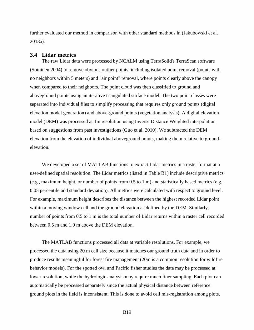
3.4 Lidar metrics The raw Lidar data were processed by NCALM using TerraSolid's TerraScan software

(Soininen 2004) to remove obvious outlier points, including isolated point removal (points with

no neighbors within 5 meters) and "air point" removal, where points clearly above the canopy

when compared to their neighbors. The point cloud was then classified to ground and

aboveground points using an iterative triangulated surface model. The two point classes were

separated into individual files to simplify processing that requires only ground points (digital

elevation model generation) and above-ground points (vegetation analysis). A digital elevation

model (DEM) was processed at 1m resolution using Inverse Distance Weighted interpolation

based on suggestions from past investigations (Guo et al. 2010). We subtracted the DEM

elevation from the elevation of individual aboveground points, making them relative to ground-

elevation.

We developed a set of MATLAB functions to extract Lidar metrics in a raster format at a

user-defined spatial resolution. The Lidar metrics (listed in Table B1) include descriptive metrics

(e.g., maximum height, or number of points from 0.5 to 1 m) and statistically based metrics (e.g.,

0.05 percentile and standard deviation). All metrics were calculated with respect to ground level.

For example, maximum height describes the distance between the highest recorded Lidar point

within a moving window cell and the ground elevation as defined by the DEM. Similarly,

number of points from 0.5 to 1 m is the total number of Lidar returns within a raster cell recorded

between 0.5 m and 1.0 m above the DEM elevation.

The MATLAB functions processed all data at variable resolutions. For example, we

processed the data using 20 m cell size because it matches our ground truth data and in order to

produce results meaningful for forest fire management (20m is a common resolution for wildfire

behavior models). For the spotted owl and Pacific fisher studies the data may be processed at

lower resolution, while the hydrologic analysis may require much finer sampling. Each plot can

automatically be processed separately since the actual physical distance between reference

ground plots in the field is inconsistent. This is done to avoid cell mis-registration among plots.

B20

In other words, each individual plot raster is generated based on the position of its plot center in

such a way that the central pixel precisely overlaps the plot center.

In addition, we appended topographical information based on the DEM derived from the

Lidar data. All topographical measures (listed in Table B1) were derived from the DEM using

ITT's ENVI 4.5 Topographical Modeling feature (ITT Visual Information Solutions 2009). The

plot rasters described above and the topographical information were combined into a raster

dataset (Lidar data cube, or the LDC) with a set of bands similar to a hyperspectral image cube,

where each band describes different Lidar data or topography metrics. The LDC is saved in the

Tagged Image File Format (TIFF) raster format to increase compatibility with external analysis

software. An ENVI header file is generated to preserve metadata and description of each metric.

All metrics are listed in Table B1.

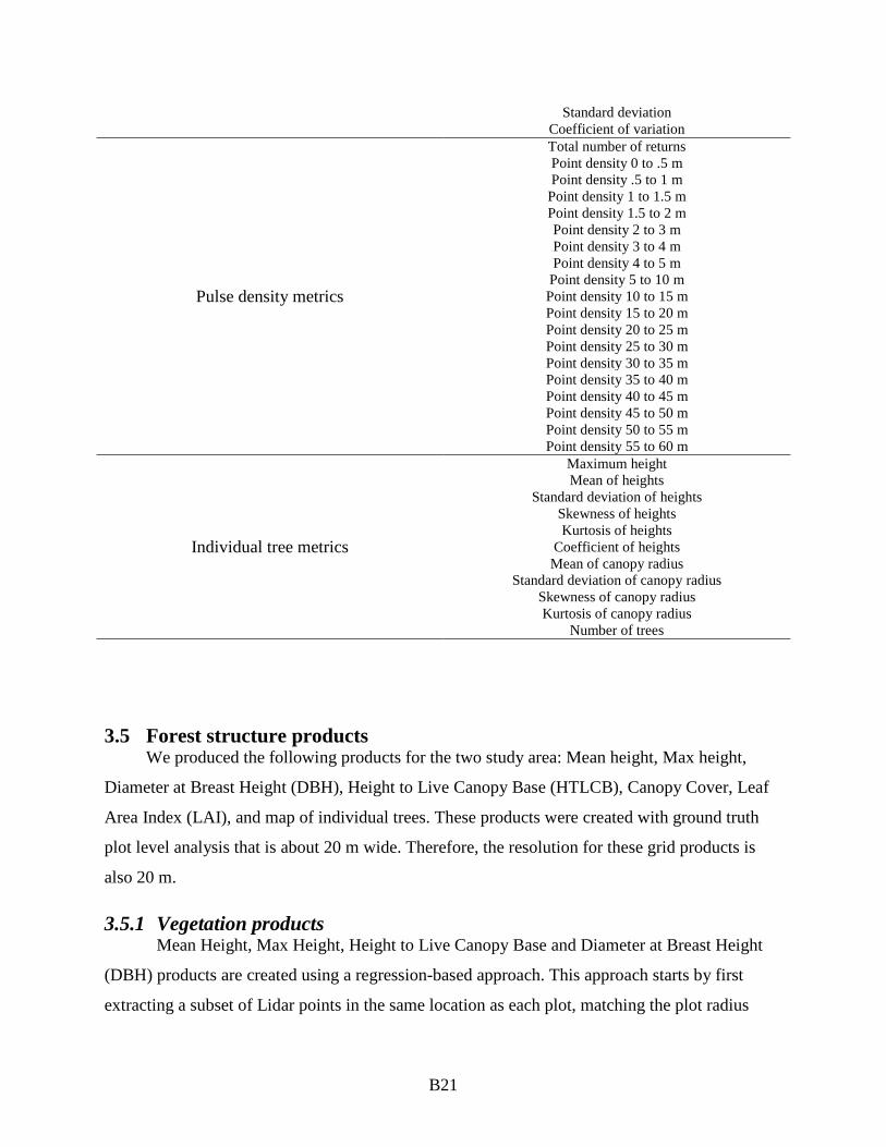
Table B1: Example of all metrics extracted from Lidar data, used to create forest structure and other products with regression.

Topographic variables 1m, 10, 20m Elevation

Slope Aspect

Topographic variables 1m

Profile convexity Planar convexity

Longitudinal convexity Cross-sectional convexity

Minimum curvature Maximum curvature

Height metrics

Height: minimum Height: mean

Height: maximum Height: standard deviation

Skewness of heights Kurtosis of heights

Coefficient of heights Quadradic mean of heights

Lorey’s height (modeled variable)

Percentile metrics

Percentile 0.01 Percentile 0.05 Percentile 0.10 Percentile 0.25 Percentile 0.50 Percentile 0.75 Percentile 0.90 Percentile 0.95 Percentile 0.99

Minimum Maximum

Mean

B21

Standard deviation Coefficient of variation

Pulse density metrics

Total number of returns Point density 0 to .5 m Point density .5 to 1 m

Point density 1 to 1.5 m Point density 1.5 to 2 m Point density 2 to 3 m Point density 3 to 4 m Point density 4 to 5 m

Point density 5 to 10 m Point density 10 to 15 m Point density 15 to 20 m Point density 20 to 25 m Point density 25 to 30 m Point density 30 to 35 m Point density 35 to 40 m Point density 40 to 45 m Point density 45 to 50 m Point density 50 to 55 m Point density 55 to 60 m

Individual tree metrics

Maximum height Mean of heights

Standard deviation of heights Skewness of heights Kurtosis of heights

Coefficient of heights Mean of canopy radius

Standard deviation of canopy radius Skewness of canopy radius Kurtosis of canopy radius

Number of trees

3.5 Forest structure products We produced the following products for the two study area: Mean height, Max height,

Diameter at Breast Height (DBH), Height to Live Canopy Base (HTLCB), Canopy Cover, Leaf

Area Index (LAI), and map of individual trees. These products were created with ground truth

plot level analysis that is about 20 m wide. Therefore, the resolution for these grid products is

also 20 m.

3.5.1 Vegetation products Mean Height, Max Height, Height to Live Canopy Base and Diameter at Breast Height

(DBH) products are created using a regression-based approach. This approach starts by first

extracting a subset of Lidar points in the same location as each plot, matching the plot radius

B22

(12.62 m). The Lidar points were normalized by subtracting the ground points (DEM) from the

extracted Lidar points. A height profile is created on the normalized points using the following

groups: z values for minimum, percentiles (1st, 5th, 10th, 25th, 50th, 75th, 90th, 95th, 99th),

maximum, mean, standard deviations and the coefficient of variation.

The Lidar-based predictors (height profile) are fitted against the field measurements by

stepwise regression modeling (Andersen et al., 2005). The best models are then applied to the

entire study area. This is done by iterating through each pixel of the product grid, extracting

Lidar points that fall within that pixel and calculating the pixel value using the relation found in

the previously mentioned analysis.

3.5.2 Canopy cover Canopy Cover (CC) is determined by analyzing the canopy height model (CHM). CHMs

typically have a resolution of 1 m, and the canopy covers have a resolution of 20 m. Each pixel

in the canopy cover grid is iterated and CHM pixel values that fall within the canopy cover pixel

are extracted. The value of the canopy cover pixel is calculated as the ratio of CHM pixels that

have a value above a threshold to the total number of extracted pixels from the CHM (Lucas et

al. 2006). The height threshold of 1.5 m is used to differentiate between trees and shrubs.

3.5.3 Leaf area index The leaf area index (LAI) product is created using the Lidar vegetation points,

normalized by the DEM. Each pixel in the LAI grid is iterated and Lidar points that fall within

the pixel are extracted. An average scan angle is calculated using the extracted Lidar points and

the following equation:

nangle

angn

i i∑== 1

where 𝑎𝑎𝑎 is the average scan angle, n is the number of extracted points and anglei is the scan

angle for a single extracted point i. Next the gap fraction (𝐺𝐺) is calculated using the following

equation:

B23

nn

GF ground=

where nground is the number of extracted points that have a z value smaller than 1.5 m (equivalent

to the height of a hemispherical camera) and n is the total number of extracted points. Finally,

the LAI value is calculated using the following equation:

kGFangLAI )ln()cos( ×

−=

where 𝐿𝐿𝐿 is the extinction coefficient and ln is the natural logarithm (Richardson et al. 2009).

The value 0.5 is used for the extinction coefficient k, as suggested in the literature (Richardson et

al. 2009).

3.6 Fire behavior modeling inputs Forest fire behavior models need a variety of spatial data layers in order to accurately

predict forest fire behavior, including elevation, slope, aspect, canopy height, canopy cover,

crown base height, crown bulk density, as well as a layer describing the types of fuel found in the

forest (called the “fuel model”). These spatial data layers are not often developed using Lidar

data for this purpose (fire ecologists typically use field-sampled data), and so we explored the

use of Lidar data to describe each of the forest-related variables (Jakubowski et al. 2013b). We

conducted a comprehensive examination of forest fuel models and forest fuel metrics derived

from Lidar and color infrared (CIR) imagery (CIR is often used for mapping vegetation since

plants reflect infrared light well) for use in fire behavior modeling. Specifically, we used high-

density, discrete return airborne Lidar data and National Agriculture Imagery Program (NAIP) 1-

meter resolution imagery to find the optimal combination of data input (Lidar, imagery, and their

various combinations/transforms), and method (we used three types of methods: clustering,

regression trees, or machine learning algorithms) in order to extract surface fuel models and

canopy metrics from Sierra Nevada mixed conifer forests. All Lidar-derived metrics were

evaluated by comparing them to field data and deriving correlation coefficients.

B24

3.7 Tradeoffs in Lidar density Collection of Lidar (light detection and ranging) data can be costly, and costs depend on

the density of the resulting data (pulses or “hits” per m2). The density of our Lidar product is

shown in Figure B4, where we have progressively thinned the data from 10 pulses/m2 to 0.02

pulses/m2. Most Lidar acquisitions capture the highest possible density of data (up to 12

pulses/m2); but it is not known if that level of detail is always required. The benefit of collecting

less dense data might be that data would be able to be captured over a larger area for the same

cost. We investigated the ability of different densities of Lidar data to predict forest metrics at

the plot scale (e.g., 1/5-hectare or ½-acre).

We examined ten

canopy metrics

(maximum and mean

tree height, total basal

area, tree density,

mean height to live

crown base (HTLCB),

canopy cover,

maximum and mean

diameter at breast

height (DBH), and

shrub cover and height) based on varying pulse density of Lidar data – from low density

(0.01pulses/m2) to high density (10 pulses/m2). We tested the agreement between each metric

and field data across the range of Lidar densities to see when and if accuracy dropped.

3.8 Vegetation maps Accurate and up-to-date vegetation maps are critical for managers and scientists, because

they serve a range of functions in natural resource management (e.g., forest inventory, forest

treatment, wildfire risk control, and wildlife protection), as well as ecological and hydrological

modeling, and climate change studies. Traditional methods for vegetation mapping are usually

based on field surveys, literature reviews, aerial photography interpretation, and collateral and

ancillary data analysis (Pedrotti 2012). However, these methods can be very expensive and time-

consuming, and usually the vegetation maps obtained from these traditional methods are time

Figure B4: Figure showing progressively less dense Lidar point cloud from left to right.

B25

sensitive. Remote sensing has proved to be very powerful in vegetation mapping by employing

image classification techniques. Multispectral remote sensing imagery such as Landsat, SPOT,

MODIS, AVHRR, IKONOS, and QuickBird are among of the most commonly used. However,

most studies using both multispectral and hyperspectral imagery usually only focus on either

mapping the land cover type or mapping the vegetation composition. Examining the vertical

structure in forests has rarely been considered because the limited penetration capability for

multispectral and hyperspectral data. We developed a new strategy to map vegetation

communities in the SNAMP study areas by considering both the tree species composition and

vegetation vertical structure characteristics. We developed a novel unsupervised classification

scheme using an automatic cluster determination algorithm based on Bayesian Information

Criterion (BIC) and k-means classification which was applied to the Lidar and imagery data

(NAIP imagery) to map the vegetation community, and the post-hoc analysis based on field

measurements was used to define the property for each vegetation group.

3.9 Forest fuel treatment detection The planned forest fuel treatment boundaries are often geographically distinct from the

planned extents due to the operational constraints and protection of resources (e.g., perennial

streams, cultural resources, wildlife habitat, etc.). Knowing the actual (as opposed to planned)

extent of forest fuel treatments is critical for understanding how they affect wildfire risk, wildlife

and forest health. Traditionally, the method for reporting complete forest fuel treatment extent is

highly dependent on field observations, which is very labor-intensive and expensive. Moreover,

since forest fuel treatments typically focus on reducing ladder and surface fuels and decreasing

small tree density, aerial imagery with limited penetration capability through forest canopy can

be hardly used to identify their extent. In this study, we examined the capability of multi-

temporal Lidar data on forest fuel treatment detection. Our approach involved the combination

of a pixel-wise thresholding method and an object-of-interest (OBI) segmentation method.

Firstly, the differences between the pre- and post-treatment Lidar derived canopy cover were

used to represent the change information. We assumed that this change information should be

normally distributed, and the variation within the 95% confidence should be recognized as the

background information. Thus, µ +/- 1.96σ was used as the threshold to differentiate the treated

and untreated pixels, where µ and σ are the mean and standard deviation of the change image,

respectively. Finally, to further remove noise, the OBIA segmentation method was used to filter

B26

the pixel-wise result considering the fact that forest fuel treatments were usually conducted in

spatially continuous areas (Zhang et al. 2013).

4 Results 4.1 Standard Lidar products: DTM, DSM, CHM

Slope based filtering method is an efficient method to discriminant ground returns from

Lidar point cloud in areas with flat terrain. Its accuracy linearly decreases with the rise of slope.

While vegetation density has a great influence on other filtering algorithms, such as

interpolation-based filtering algorithm and morphological filtering algorithm. Fine resolution

DTM and DSM products can be interpolated from the obtained ground returns and first returns

of the Lidar point cloud. Results show that the accuracy of the interpolated DTM and DSM

products increases with the sampling density. Finally, the CHM product can be directly

calculated from the difference between the DTM and DSM (Figure B5). The accuracy of these

products is reported in Table B2.

Figure B5: Lidar-derived canopy height model (CHM): a) Last Chance study area, b) Sugar Pine study area.

4.2 Topographic products We created detailed Digital Elevation Model (DEM) products or both study sites (Figure

B6). In our investigation of different interpolation methods, our results show that simple

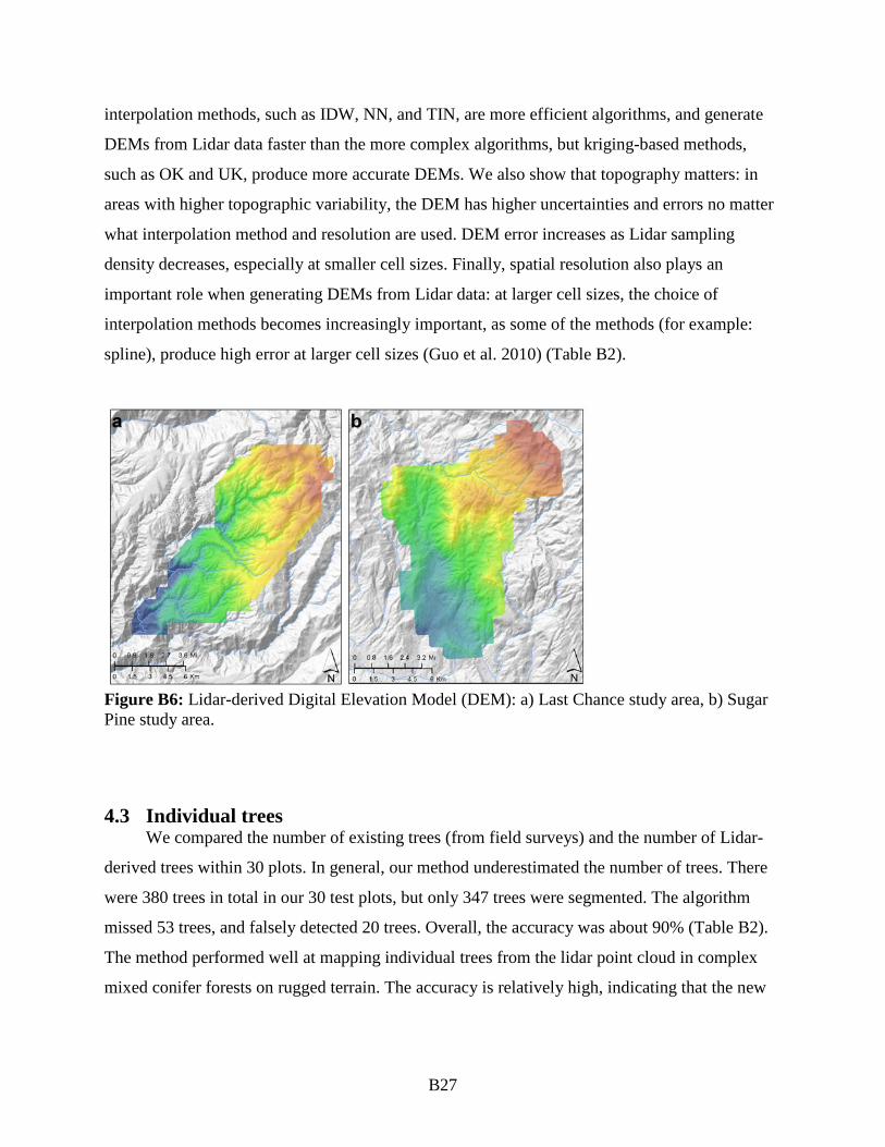
B27

interpolation methods, such as IDW, NN, and TIN, are more efficient algorithms, and generate

DEMs from Lidar data faster than the more complex algorithms, but kriging-based methods,

such as OK and UK, produce more accurate DEMs. We also show that topography matters: in

areas with higher topographic variability, the DEM has higher uncertainties and errors no matter

what interpolation method and resolution are used. DEM error increases as Lidar sampling

density decreases, especially at smaller cell sizes. Finally, spatial resolution also plays an

important role when generating DEMs from Lidar data: at larger cell sizes, the choice of

interpolation methods becomes increasingly important, as some of the methods (for example:

spline), produce high error at larger cell sizes (Guo et al. 2010) (Table B2).

Figure B6: Lidar-derived Digital Elevation Model (DEM): a) Last Chance study area, b) Sugar Pine study area.

4.3 Individual trees We compared the number of existing trees (from field surveys) and the number of Lidar-

derived trees within 30 plots. In general, our method underestimated the number of trees. There

were 380 trees in total in our 30 test plots, but only 347 trees were segmented. The algorithm

missed 53 trees, and falsely detected 20 trees. Overall, the accuracy was about 90% (Table B2).

The method performed well at mapping individual trees from the lidar point cloud in complex

mixed conifer forests on rugged terrain. The accuracy is relatively high, indicating that the new

B28

algorithm has good potential for use in other forested areas, and across broader areas than is

possible with fieldwork alone.

4.4 Lidar metrics We created a suite of Lidar metrics that were used in the creation of a range of maps and

products through various regression approaches. The accuracy of these products is summarized

below in Table B2.

4.5 Forest structure products Mean height, max height, DBH, HTLCB, canopy cover, and LAI products were made for

both sites. The product showing canopy cover for both sites is in Figure B7.

Figure B7: Lidar-derived canopy cover: a) Last Chance study area, b) Sugar Pine study area.

4.6 Fire behavior modeling inputs Specific surface forest “fuel models” (these are detailed descriptions like “dwarf conifer

with understory” or “low load compact conifer litter”) proved difficult to predict in this dense

forest environment, although general fuel types (such as predominantly shrub, or mostly timber)

were estimated with reasonable (up to 76% correct) accuracy because fewer of the light energy

from the Lidar penetrated to the forest floor in denser forests, making accurate characterization

of understory shrubs more difficult. The predictive power of canopy metrics increases as we

describe metrics higher up in the canopy. The accuracy—in terms of Pearson’s correlation

B29

coefficient—ranged from 0.87 for estimating canopy height, through 0.62 for shrub cover, to

0.25 for canopy base height.

4.7 Tradeoffs in Lidar density The accuracy of the Lidar predictions for all ten metrics increased as the Lidar density

increased from 0.01 pulses/m2 to 1 pulse/m2. However, the accuracy of many of the metrics

showed very little improvement after that. Metrics that described forest cover (e.g., forest canopy

and shrub cover) required higher densities of Lidar data to be mapped accurately. In general, the

results confirm findings from previous studies: the overall accuracy of a predicted forest

structure metric decreased roughly with its vertical position within the canopy: metrics that

estimate the tops of forests are more accurately mapped with Lidar than those in the middle of

the canopy or on the forest floor and so require less dense data for most applications (Jakubowski

et al. 2013c).

Many plot-scale forest canopy measures (e.g., maximum and mean tree height, total basal

area, maximum and mean diameter at breast height (DBH)) are well predicted with moderate

density Lidar data: 1 pulse/m2. More detailed features, such as individual trees, would likely

require high-density Lidar data. Coverage metrics (canopy cover, tree density, and shrub cover)

were more sensitive to pulse density.

4.8 Vegetation maps The vegetation map created for each site shows complex and unique vegetation structure

characteristics and vegetation species composition. The overall accuracy and kappa coefficient of

the vegetation mapping results are over 78% and 0.64 for both study sites. The vegetation map

product, and in particular the boundaries of forest stands created was used by the FFEH Team in

their fire behavior modeling work.

4.9 Forest fuel treatment extent The forest fuel treatment detection result is well in agreement with the proposed forest

treatment operation extent. By assessing with the field observations, the result also shows a

satisfactory accuracy. The overall accuracy is 93.5% and the kappa coefficient is 0.70. Although

there are some detected treated areas are not within the proposed forest treatment operation

extents, most of them may have been treated based on field observations and direct Lidar point

B30

cloud comparison. Figure B8 shows a direct comparison between the pre-treatment and post-

treatment Lidar point cloud. Moreover, the same forest treatment detection routine was also

applied on airborne imagery. Results show that Lidar derived canopy cover outperformed the

aerial image and is more robust to detect light forest treatment areas. Accuracy of all products is

listed in Table B2.

Figure B8: An example of direct point cloud comparison in an area with forest fuel treatments.

B31

Table B2: Accuracy results for most of the products created by the SNAMP Spatial Team.

Product Type/Method Accuracya SNAMP Publication

Standard Lidar products DTMb Derived from Lidar point

cloud 20-30 cm NCALM

report DSMb Derived from Lidar point

cloud 20-30cm NCALM

report CHMb Direct: from DTM + DEM 20-30 cm NCALM

report Topographic products

DEMb Direct, from DTM 20-30 cm #4 Individual trees

Individual trees Derived from Lidar point cloud

90% #6

Individual trees Derived from Lidar + imagery 0.91 - 0.95 #24 Forest structure products (20m)

Mean height Indirect: from regression 0.67 Max height Indirect: from regression 0.78

DBH Indirect: from regression 0.61 HTLCB Indirect: from regression 0.62

Canopy Cover Indirect: from regression 0.62 LAI Direct Not

measured

Fire behavior modeling inputs (20m) Canopy height (max) Indirect: from regression 0.87 #13

Canopy cover Indirect: from regression 0.83 #13 Total basal area Indirect: from regression 0.82 #13

Shrub cover Indirect: from regression 0.62 #13 Canopy height (mean) Indirect: from regression 0.60 #13

Shrub height Indirect: from regression 0.59 #13 Canopy base height Indirect: from regression 0.41 #13

Canopy bulk density Indirect: from regression 0.25 #13 Combined fuel loads Indirect: from regression 0.48 #13

Fuel bed depth Indirect: from regression 0.35 #13 Vegetation map

Vegetation map Derived from Lidar + imagery 78% Publication to be submitted

a Accuracy is listed as best r2, unless otherwise noted. b The accuracy of DTM, DSM, CHM, and DEM were evaluated by the ground measured GPS transects data provided by NCLAM. All other vegetation-related products were evaluated by in-situ measurements.

B32

5 Discussion Mapping has always been critical for forest inventory, fire management planning, and

conservation planning. Understanding the structure of forests – tree density, volume and height

characteristics - is critical for management, fire prediction, biomass estimation, and wildlife

assessment. In California, these tasks are particularly challenging, as our forests exhibit

tremendous variability in composition, volume, quality, and topography. Optical remote sensors

such as Landsat, despite their synoptic and timely views, do not provide sufficiently detailed

depictions of forest structure for all forest management needs. We anticipate that Lidar will

continue to play an increasingly important role for forest managers interested in mapping forests

at fine detail. We discuss our broader findings in the following five areas.

5.1 Lidar maps and products Lidar data can produce a range of mapped product that in many cases more accurately map

forest height, structure and species than optical imagery alone. Mapped products include

topographic maps, locations of individual trees, forest height, canopy cover, shrub cover, fuels,

and detailed species, among other variables. Accuracies in these products ranged greatly;

generally the closer to the ground the lower the accuracy, especially in dense canopy. Many of

these mapped products can be produced at a range of spatial resolutions, from 1m to 20m and

larger. The 20m resolution adequately matches the approximate resolution of a 12.54m radius

plot.

However, Lidar data can be large in size, and there are few commonly used and easy-to-

use software packages to produce the products. Our work required a range of tools, most of them

requiring specialized coding in python, Matlab and other languages and software packages.

Moreover, although Lidar data can be used to generate maps that depict accurate forest

structure, the lack of spectral reflectance data makes the production of vegetation maps with

Lidar data alone difficult. The recorded intensity information of the Lidar data cannot be used to

reflect the forest surface reflectance characteristics due to the influence of the multi-path effect.

Our work indicated that the combination of high resolution multi-spectral aerial/satellite imagery

and lidar data is very helpful in mapping vegetation communities as well as characterizing forest

structure zones.

B33

5.2 Wildlife Lidar is an effective tool for mapping important potential forest habitat variables – such as

individual trees, tree sizes, and canopy cover - for sensitive species (Temple et al., 2015). We

believe that Lidar can help forest managers and scientists in the assessment of wildlife–habitat

relationships and conservation of important wildlife species by allowing managers to better

identify habitat characteristics on a large scale. More work can be done to link Lidar products

with CWHR habitat classes. More work needs to be done to define a particular set of habitat

characteristics that can be measured or estimated by lidar, e.g., particular height, density,

overstory/understory, and biomass criteria.

5.3 Forest management The accurate identification and quantification of individual trees from discrete Lidar pulses

typically requires high-density data. Standard plot-level metrics such as tree height, canopy

cover, and some fuel measures can reliably be derived from less dense Lidar data. However,

standard Lidar products do not yet operationally meet the requirements of forest managers who

need detailed measures of forest structure that include understanding of forest heterogeneity, and

understanding of forest change. Additionally, typical forest management metrics such as leaf

area index (LAI), quadratic mean diameter (QMD), trees per acre (TPA) are not commonly

created, nor easily validated using Lidar data.

Our work on Lidar density might help managers evaluate tradeoffs between Lidar density,

cost and coverage: if a manager needs plot-scale forest measurements (i.e., measurements

summarized at scale around ½-acre or 1/5-hectare), they might be able to cover a larger area with

lower density Lidar data for the same cost as high density Lidar data over a smaller area.

Forest fuel treatments are among the main forest management activities used to reduce the

wildfire risks. However, planned forest fuel treatment boundaries are often geographically

distinct from the planned extents due to the operational constraints and protection of resources

(e.g., perennial streams, cultural resources, wildlife habitat, etc.). Lidar derived multi-temporal

canopy cover products are highly sensitive the forest changes brought by the forest fuel

treatment, and therefore can be used to accurately map the fuel treatment extent.

B34

5.4 Fire behavior modeling While there is great promise for the use of Lidar in fire behavior models, there is more

work necessary before Lidar data can be operationally included into common fire behavior

models. Discrete return Lidar cannot accurately capture all forest structural features near the

ground when the canopy is very dense.

5.5 Biomass Our work suggests that airborne Lidar data provide the most accurate estimates of forest

biomass, but rigorous procedures should be taken in selecting appropriate allometric equations to

use as reference biomass estimates. We also showed that Lidar data when fused with course

scale, fine temporal resolution imagery such as MODIS, can be used to estimate regional scale

above ground forest biomass.

6 Resource-specific management implications and recommendations Our work using Lidar and other remote sensing products contributes to the current

discussion around the use of mapping for forest management. We discuss several management

implications here.

6.1 Lidar maps and products

6.1.1 Management implications • Lidar data can produce a range of mapped product that in many cases more accurately

map forest height, structure and species than optical imagery alone.

• Lidar software packages are not yet as easy to use as the typical desktop GIS software.

• There are known limitations with the use of discrete Lidar for forest mapping - in

particular, smaller trees and understory are difficult to map reliably.

• The fusion of hyperspectral imagery with Lidar data may be very useful to create detailed

and accurate forest species maps.

B35

6.2 Wildlife

6.2.1 Management implications • Lidar is an effective tool for mapping important forest habitat variables – such as

individual trees, tree sizes, and canopy cover - for sensitive species.

• Lidar will increasingly be used by wildlife managers, but there remain numerous

technical and software barriers to widespread adoption. Efforts are still needed to link

Lidar data, metrics and products to measures more commonly used by managers such as

CWHR habitat classes.

6.3 Fire behavior modeling

6.3.1 Management implications • Lidar data are not yet operationally included into common fire behavior models, and

more work should be done to understand error and uncertainty produced by Lidar

analysis.

6.4 Forest management

6.4.1 Management implications • There is a trade-off between detail, coverage and cost with Lidar. The accurate

identification and quantification of individual trees from discrete Lidar pulses typically

requires high-density data. Standard plot-level metrics such as tree height, canopy cover,

and some fuel measures can reliably be derived from less dense Lidar data.

• Standard Lidar products do not yet operationally meet the requirements of forest

managers who need detailed measures of forest structure that include understanding of

forest heterogeneity, and understanding of forest change. More work is needed to

translate between the remote sensing community and the forest management community

to ensure that Lidar products are useful to and used by forest managers.

• Discrete Lidar can be used to map the extent of forest fuel treatments. However, the

method of treatment (e.g., mastication, thinned, cable thinned) cannot be detected using

discrete Lidar data due to its limitation of understory forest.

The future of Lidar for forest applications will depend on a number of considerations. These

include: 1) costs, which have been declining; 2) new developments to address limitations with

B36

discrete Lidar, such as the use of waveform data; 3) new analytical methods and more easy-to-

use software to deal with increasing data sizes, particularly with regard to Lidar and optical

imagery fusion; and 4) the ability to train forest managers and scientists in Lidar data workflow

and appropriate software.

B37

7 References Aguilar, F.J., Agüera, F., Aguilar, M.A. and Carvajal, F., 2005. Effects of terrain morphology,

sampling density, and interpolation methods on grid DEM accuracy. Photogrammetric Engineering & Remote Sensing. 71(7): 805-816.

Andersen, H.-E., McGaughey, R.J. and Reutebuch, S.E., 2005. Estimating forest canopy fuel

parameters using LIDAR data. Remote Sensing of Environment. 94: 441-449. Anderson, E.S., Thompson, J.A. and Austin, R.E., 2005. LiDAR density and linear interpolator

effects on elevation estimates. International Journal of Remote Sensing. 26(18): 3889-3900.

Anderson, J.E., Plourde, L.C., Martin, M.E., Braswell, B.H., Smith, M.-L., Dubayah, R.O.,

Hofton, M.A. and d, J.B.B., 2008. Integrating waveform lidar with hyperspectral imagery for inventory of a northern temperate forest Remote Sensing of Environment. 112: 1856-1870.

Blanchard, S., M. Jakubowski and Kelly, M., 2011. Object-based image analysis of downed logs

in a disturbed forest landscape using lidar. Remote Sensing. 3(11): 2420-2439. Chen, Q., Baldocchi, D., Gong, P. and Kelly, M., 2006. Isolating individual trees in a savanna

woodland using small footprint LIDAR data. Photogrammetric Engineering and Remote Sensing. 72(8): 923-932.

Dubayah, R. and Drake, J., 2000. Lidar remote sensing for forestry. Journal of Forestry. 98(6):

44-46. Finney, M.A., 1995. FARSITE fire area simulator. Systems for Environmental Management,

Missoula, MT. Finney, M.A., 1998. FARSITE: Fire Area Simulator - Model development and evaluation. Usda

Forest Service Rocky Mountain Forest and Range Experiment Station Research Paper(RP-4): 1-+.

Garcia-Feced, C., Temple, D.J. and Kelly, M., 2012. Characterizing California Spotted Owl nest

sites and their associated forest stands using Lidar data. Journal of Forestry. 108(8): 436-443.

Gatziolis, D. and Andersen, H.-E., 2008. A Guide to LIDAR Data Acquisition and Processing

for the Forests of the Pacific Northwest, Department of Agriculture Forest Service. Pacific Northwest Research Station.

Guo, Q., Li, W., Yu, H. and Alvarez, O., 2010. Effects of Topographic Variability and Lidar

Sampling Density on Several DEM Interpolation Methods. Photogrammetric Engineering & Remote Sensing. 76(6): 701-712.

B38

Henning, J.G. and Radtke, P.J., 2006. Detailed stem measurements of standing trees from

ground-based scanning lidar. Forest Science. 52(1): 67-80. ITT Visual Information Solutions, 2009. ENVI software. http://www.ittvis.com/ENVI. Jakubowski, M.J., Li, W., Guo, Q. and Kelly, M., 2013a. Delineating individual trees from lidar

data: a comparison of vector- and raster-based segmentation approaches. Remote Sensing. 5(4163-4186).

Jakubowski, M.K., Guo, Q., Collins, B., Stephens, S. and Kelly, M., 2013b. Predicting surface

fuel models and fuel metrics using lidar and imagery in dense, mountainous forest. Photogrametric Engineering & Remote Sensing. 79(1): 37-49.

Jakubowski, M.K., Guo, Q. and Kelly, M., 2013c. Tradeoffs between lidar pulse density and

forest measurement accuracy. Remote Sensing of Environment 130: 245-253. Kelly, M. and Tommaso, S.D., 2015. Mapping forests with Lidar provides flexible, accurate data

with many uses. California Agriculture. 69(1): 14-20. Leckie, D., Gougeon, F., Hill, D., Quinn, R., Armstrong, L. and Shreenan, R., 2003. Combined

high-density lidar and multispectral imagery for individual tree crown analysis. Canadian Journal of Remote Sensing. 29(5): 633-649.

Lefsky, M.A., Cohen, W.B., Parker, G.G. and Harding, D.J., 2002. Lidar remote sensing for

ecosystem studies. BioScience. 52(1): 19-30. Li, W., Guo, Q., Jakubowski, M. and Kelly, M., 2012. A new method for segmenting individual

trees from the lidar point cloud. Photgrammetric Engineering and Remote Sensing. 78(1): 75-84.

Lucas, R.M., Cronin, N., Lee, A., Moghaddam, M., Witte, C. and Tickle, P., 2006. Empirical

relationships between AIRSAR backscatter and LiDAR-derived forest biomass, Queensland, Australia. Remote Sensing of Environment. 100(3): 407-425.

Mutlu, M., Popescu, S.C., Stripling, C. and Spencer, T., 2008. Mapping surface fuel models

using lidar and multispectral data fusion for fire behavior. Remote Sensing of Environment. 112: 274-285.

Naesset, E., 2004. Practical large-scale forest stand inventory using a small-footprint airborne

scanning laser. Scandinavian Journal of Forest Research. 19: 164-179. Naesset, E. and Bjerknes, K.-O., 2001. Estimating tree heights and number of stems in young

forest stands using airborne laser scanning data. Remote Sensing of Environment. 78: 328-340.

B39

Naesset, E. and Gobakken, T., 2008. Estimation of above- and blow-ground biomass across regions of the boreal forest zone using airborne laser. Remote Sensing of Environment. 112: 3079-3090.

Ørka, H.O., Næsset, E. and Bollandsås, O.M., 2007. Utilizing airborne laser intensity for tree

species classification, ISPRS Workshop on Laser Scanning 2007 and SilviLaser 2007, Finland.

Pedrotti, F., 2012. Plant and vegetation mapping, 1. Springer Science & Business Media. Pesonen, A., Maltamo, M., inen, K.E. and n, P.P., 2008. Airborne laser scanning-based

prediction of coarse woody debris volumes in a conservation area Forest Ecology & Management. 255: 3288-3296.

Popescu, S.C. and Wynne, R.H., 2004. Seeing the trees in the forest: using lidar and

multispectral data fusion with local filtering and variable window size for estimating tree height. Photogrammetric Engineering & Remote Sensing. 70(5): 589-604.

Popescu, S.C., Wynne, R.H. and Scrivani, J.A., 2004. Fusion of small-footprint lidar and

multispectral data to estimate plot-level volume and biomass in deciduous and pine forests in Virginia, USA. Forest Science. 50(4): 551-565.

Popescu, S.C. and Zhao, K., 2008. A voxel-based lidar method for estimating crown base height

for deciduous and pine trees. Remote Sensing of Environment. 112: 767-781. Raber, G.T., Jensen, J.R., Hodgson, M.E., Tullis, J.A., Davis, B.A. and Berglund, J., 2007.

Impact of lidar nominal post-spacing on DEM accuracy and flood zone delineation. Photogrammetric Engineering and Remote Sensing. 73(7): 783-791.

Radtke, P.J. and Bolstad, P.V., 2001. Laser point-quadrat sampling for estimating foliage-height

profiles in broad-leaf forests. Canadian Journal of Forest Research. 31: 410-418. Riano, D., Meier, E., Allgower, B., Chuvieco, E. and Ustin, S.L., 2003. Modeling airborne laser

scanning data for the spatial generation of critical forest parameters in fire behavior modeling Remote Sensing of Environment. 86: 177-186.

Richardson, J.J., Moskal, L.M. and Kim, S.-H., 2009. Modeling approaches to estimate effective

leaf area index from aerial discrete-return LIDAR. Agricultural and Forest Meteorology. 149(6): 1152-1160.

Roth, B.E., Slatton, K.C. and Cohen, M.H., 2007. On the ptoential for high-resolution lidar to

improve rainfall interception estimates in forest ecosystems. Frontiers in Ecology and the Environment. 5(8): 421-428.

Soininen, A., 2004. Terra Scan for MicroStation, User's Guide. Terrasolid Ltd., Jyvaskyla,

Finland.

B40

Tao, S., Li, L., Guo, Q., Li, L., Xue, B., Kelly, M., Li, W., Xu, G. and Su, Y., 2014. Airborne

Lidar-derived volume metrics for aboveground biomass estimation: A comparative assessment for conifer stands. Agriculture and Forest Management. Agriculture and Forest Management. 189-199: 24-32.

Tempel, D.J., Gutierrez, R.J., Battles, J.J., Fry, D.L., Su. Y., Guo., Q., Reetz, M., Whitmore,

S.A., Jones, G.M., Collins, B.M., Stephens, S.L., Kelly, M., Berigan W.J., and Perry, M.Z., 2015. Evaluting short- and long-term impacts of fuels treatments and simulated wildfire on an old-forest species. Ecoshpere (accepted).

Thompson, J.A., Bell, J.C. and Butler, C.A., 2001. Digital elevation model resolution: effects on

terrain attribute calculation and quantitative soil-landscape modeling. Geoderma. 100: 67-89.

Vierling, K.T., Vierling, L.A., Gould, W.A., Martinuzzi, S. and Clawges, R.M., 2008. Lidar:

shedding new light on habitat characterization and modeling. Frontiers for Ecology and the Environment. 6(2): 90-98.

Zhang, X., Xiao, P. and Feng, X., 2013. Impervious surface extraction from high-resolution

satellite image using pixel-and object-based hybrid analysis. International Journal of Remote Sensing. 34(12): 4449-4465.

Zhao, F., Guo, Q. and Kelly, M., 2012a. Allometric equation choice impacts lidar-based forest

biomass estimates: A case study from the Sierra National Forest, CA. Agricultural and Forest Meteorology. 165: 64-72.

Zhao, F., Sweitzer, R.A., Guo, Q. and Kelly, M., 2012b. Characterizing habitats associated with

fisher den structures in the Southern Sierra Nevada, California using discrete return lidar. Forest Ecology & Management. 280: 112-119.

Zhao, K., Popescu, S. and Nelson, R., 2009. Lidar remote sensing of forest biomass: A scale-

invariant estimation approach using airborne lasers Remote Sensing of Environment. 113: 182-196.

Zimble, D.A., Evans, D.L., Carlson, G.C., Parker, R.C., Grado, S.C. and Gerard, P.D., 2003.

Characterizing vertical forest structure using small-footprint airborne LiDAR. Remote Sensing of Environment. 87: 171-182.

B41

8 Spatial Team Appendices 8.1 Appendix B1: Spatial Team publications

SNAMP PUB #4: Guo, Li, Yu, and Alvarez. 2010. Effects of topographic variability and Lidar sampling density on several DEM interpolation methods. Photogrammetric Engineering and Remote Sensing 76(6): 701–712.

Abstract: We used Lidar data to create a detailed digital elevation model for our two study sites. We investigated five different interpolation methods to create the DEMs. We examined how topography, sampling density, and spatial resolution affected accuracy of the DEMs. We found that simple interpolation models are more efficient and faster in creating DEMs, but more complex interpolation models are more accurate, but slower. We found that DEMs are less accurate in areas with more complex topography. We found that DEM error also increases as Lidar sampling density decreases. We found that some of the interpolation methods do not work well with larger cell sizes. These results might be helpful to guide the choice of appropriate Lidar interpolation methods for DEM generation.

SNAMP PUB #5: Garcia-Feced, Tempel, and Kelly. 2011. Lidar as a tool to characterize wildlife habitat: California spotted owl nesting habitat as an example. Journal of Forestry 108(8): 436-443.

Abstract: We demonstrate the use of an emerging technology, airborne light detection and ranging (Lidar), to assess forest wildlife habitat by showing how it can improve the characterization of California spotted owl (Strix occidentalis occidentalis) nesting habitat. Large residual trees are important elements for many wildlife species and often, apparently, facilitate selection of habitat by spotted owls. However, we currently lack the ability to identify such trees over large spatial scales. We acquired multiple-return, high-resolution Lidar data for a 107.1-km2 area in the central Sierra Nevada, California. We surveyed for spotted owls within this area during 2007−2009 and located 4 nest trees. We then used the Lidar data to measure the number, density and pattern of residual trees (≥ 90 cm dbh) and to estimate canopy cover within 200 m of four nest trees. Nest trees were surrounded by large numbers of residual trees and high canopy cover. We believe that Lidar would greatly benefit forest managers and scientists in the assessment of wildlife-habitat relationships and conservation of important wildlife species.

SNAMP PUB #6: Li, Guo, Jakubowski, and Kelly. 2012. A new method for segmenting individual trees from the Lidar point cloud. Photogrammetric Engineering and Remote Sensing 78(1): 75-84.

Abstract: Light Detection and Ranging (Lidar) has been widely applied to characterize the 3-dimensional (3D) structure of forests as it can generate 3D point data with high spatial resolution and accuracy. Individual tree segmentations, usually derived from the canopy height model, are used to derive individual tree structural attributes such as tree

B42

height, crown diameter, canopy-based height, and others. In this study we develop a new algorithm to segment individual trees from the small footprint discrete return airborne Lidar point cloud. The new algorithm adopts a top-to-bottom region growing approach that segments trees individually and sequentially from the tallest to the shortest. We experimentally applied the new algorithm to segment trees in a mixed coniferous forest in the Sierra Nevada Mountains in California, USA. The results were evaluated in terms of recall, precision, and F-score, and show that the algorithm detected 86% of the trees (“recall”), 94% of the segmented trees were correct (“precision”), and the overall F-score is 0.9. Our results indicate that the proposed algorithm has good potential in segmenting individual trees in mixed conifer stands of similar structure using small footprint, discrete return Lidar data.

SNAMP PUB #7: Blanchard, Jakubowski, and Kelly. 2011. Object-Based Image Analysis of Downed Logs in Disturbed Forested Landscapes using Lidar. Remote Sensing 3: 2420-2439.

Abstract: Downed logs on the forest floor provide habitat for species, fuel for forest fires, and function as a key component of forest nutrient cycling and carbon storage. Ground-based field surveying is a conventional method for mapping and characterizing downed logs but is limited. In addition, optical remote sensing methods have not been able to map these ground targets due to the lack of optical sensor penetrability into the forest canopy and limited sensor spectral and spatial resolutions. Lidar (light detection and ranging) sensors have become a more viable and common data source in forest science for detailed mapping of forest structure. This study evaluates the utility of discrete, multiple return airborne Lidar-derived data for image object segmentation and classification of downed logs in a disturbed forested landscape and the efficiency of rule-based object-based image analysis (OBIA) and classification algorithms. Downed log objects were successfully delineated and classified from Lidar derived metrics using an OBIA framework. 73% of digitized downed logs were completely or partially classified correctly. Over classification occurred in areas with large numbers of logs clustered in close proximity to one another and in areas with vegetation and tree canopy. The OBIA methods were found to be effective but inefficient in terms of automation and analyst’s time in the delineation and classification of downed logs in the Lidar data.

SNAMP PUB #13: Jakubowski, Guo, Collins, Stephens, and Kelly. 2013. Predicting surface fuel models and fuel metrics using Lidar and CIR imagery in a dense, mountainous forest. Photogrammetric Engineering and Remote Sensing 79(1): 37-49.

Abstract: We compared the ability of several classification and regression algorithms to predict forest stand structure metrics and standard surface fuel models. Our study area spans across a dense, topographically complex Sierra Nevada mixed-conifer forest. We used clustering, regression trees, and support vector machine algorithms to analyze high density (average 9 pulses/m2), discrete return, small footprint Lidar data, along with multispectral imagery. Stand structure metric predictions generally decreased with increased canopy penetration. For example, from the top of canopy, we predicted canopy

B43

height (r2 = 0.87), canopy cover (r2 = 0.83), BA (r2 = 0.82), shrub cover (r2 = 0.62), shrub height (r2 = 0.59), combined fuel loads (r2 = 0.48), and fuel bed depth (r2 = 0.35). While the general fuel types were predicted accurately, specific surface fuel model predictions were poor (76 percent and 50 percent correct classification, respectively) using all algorithms. These fuel components are critical inputs for wildfire behavior modeling, which ultimately support forest management decisions. This comprehensive examination of the relative utility of Lidar and optical imagery will be useful for forest science and management.

SNAMP PUB #14: Zhao, Guo, and Kelly. 2012. Allometric equation choice impacts Lidar-based forest biomass estimates: A case study from the Sierra National Forest, CA. Agriculture and Forest Meteorology 165: 64– 72.

Abstract: Plot-level estimates of biomass were derived from field data and two different allometric equations. Estimates differed between allometric equations, especially in plots with high biomass. Selection of allometric equations can influence the capacity of Lidar data to estimate biomass. The best fit between field data and Lidar data were found using a regional allometric equation and a combination of Lidar metrics and individual tree data.

SNAMP PUB #16: Zhao, Sweitzer, Guo and Kelly. 2012. Characterizing habitats associated with fisher den structures in southern Sierra Nevada forests using discrete return Lidar. Forest Ecology and Management 280: 112–119.

Abstract: This study explored the ability of Lidar-derived metrics to capture topography and forest structure surrounding denning trees used by the Pacific fisher (Martes pennanti) as a case study to illustrate the utility of Lidar remote sensing in studying mammal-habitat associations. We used Classification and Regression Trees (CART) to statistically compare the slope and Lidar-derived forest height and structure metrics in the circular area (with radius of 10–50 m) surrounding denning trees and randomly selected non-denning trees. We accessed our model accuracy using resubstitution and cross-validation methods. Our results show that there is a strong association between fisher denning activity and its surrounding forested environment across scales, with high classification accuracy (overall accuracies above 80% and cross-validation accuracies above 70%) at 20, 30 and 50 m ranges. The best classification accuracies were found at 20 m (optimal resubstitution accuracy 86.2% and cross-validation accuracy 78%). Tree height and slope were important variables in classifying the area immediately surrounding denning trees; at scales larger than 20 m, forest structure and complexity became more important.

SNAMP PUB #18: Jakubowski, Guo, and Kelly. 2013. Tradeoffs between Lidar pulse density and forest measurement accuracy. Remote Sensing of Environment 130: 245–253.

B44

Abstract: Discrete Lidar is increasingly used to analyze forest structure. Technological improvements in Lidar sensors have led to the acquisition of increasingly high pulse densities, possibly reflecting the assumption that higher densities will yield better results. In this study, we systematically investigated the relationship between pulse density and the ability to predict several commonly used forest measures and metrics at the plot scale. The accuracy of predicted metrics was largely invariant to changes in pulse density at moderate to high densities. In particular, correlations between metrics such as tree height, diameter at breast height, shrub height and total basal area were relatively unaffected until pulse densities dropped below 1 pulse/m2. Metrics pertaining to coverage, such as canopy cover, tree density and shrub cover were more sensitive to changes in pulse density, although in some cases high prediction accuracy was still possible at lower densities. Our findings did not depend on the type of predictive algorithm used, although we found that support vector regression (SVR) and Gaussian processes (GP) consistently outperformed multiple regression across a range of pulse densities. Our results suggest that low-density Lidar data may be capable of estimating typical forest structure metrics reliably in some situations. These results provide practical guidance to forest ecologists and land managers who are faced with tradeoff in price, quality and coverage, when planning new Lidar data acquisition.

SNAMP PUB #24: Jakubowski, Li, Guo, and Kelly. 2013. Delineating individual trees from Lidar data: a comparison of vector- and raster-based segmentation approaches. Remote Sensing 5: 4163-4186

Abstract: This work concentrates on delineating individual trees from discrete Lidar data in topographically-complex, mixed conifer forest across the California’s Sierra Nevada. We delineated individual trees using vector data and a 3D Lidar point cloud segmentation algorithm, and using raster data with an object-based image analysis (OBIA) of a canopy height model (CHM). The two approaches are compared to each other and to ground reference data. We used high density (9 pulses/m2), discreet Lidar data and WorldView-2 imagery to delineate individual trees, and to classify them by species or species types. We also identified a new method to correct artifacts in a high-resolution CHM. Our main focus was to determine the difference between the two types of approaches and to identify the one that produces more realistic results. We compared the delineations via tree detection, tree heights, and the shape of the generated polygons. The tree height agreement was high between the two approaches and the ground data (r2: 0.93–0.96). Tree detection rates increased for more dominant trees (8-100 percent). The two approaches delineated tree boundaries that differed in shape: the Lidar-approach produced fewer, more complex, and larger polygons that more closely resembled real forest structure.

SNAMP PUB #29 Tao, Guo, Li, Xue, Kelly, Li, Xu, and Su. 2015. Airborne Lidar-derived volume metrics for aboveground biomass estimation: a comparative assessment for conifer stands. Agricultural and Forest Meteorology 198–199: 24–3

B45

Abstract: Estimating aboveground biomass (AGB) is essential to quantify the carbon balance of terrestrial ecosystems, and becomes increasingly important under changing global climate. Volume metrics of individual trees, for example stem volume, have been proven to be strongly correlated to AGB. In this paper, we compared a range of airborne Lidar-derived volume metrics (i.e., stem volume, crown volume under convex hull, and crown volume under Canopy Height Model (CHM)) to estimate AGB. In addition, we evaluated the effect of horizontal crown overlap (which is often neglected in Lidar literature) on the accuracy of AGB estimation by using a hybrid method that combined marker-controlled watershed segmentation and point cloud segmentation algorithms. Our results show that: 1) when the horizontal crown overlap issue was not addressed, models based on point cloud segmentation outperformed models based on marker-controlled watershed segmentation; models using stem volume estimated AGB more accurately than models using crown volume under convex hull and crown volume under CHM. 2) Once the horizontal crown overlap issue was taken into consideration, the model using crown volume under individual trees in the Lidar cloud CHM yielded a more accurate estimation of AGB. Our study provides a comprehensive evaluation of the use of airborne Lidar-derived volume metrics for AGB estimation and could help researchers choose the appropriate airborne Lidar-derived volume metric. Moreover, the results also indicate that horizontal crown overlap should be addressed when the airborne Lidar-derived forest crown volume is used for estimating AGB.

SNAMP PUB #37 Li, Guo, Tao, Kelly, and Xu. Lidar with multi-temporal MODIS provide a means to upscale predictions of forest biomass. ISPRS Journal of Photogrammetry and Remote Sensing.

Abstract: Accurate estimation of forest AGB has become increasingly important for a wide range of end-users. Although satellite remote sensing provides abundant observations to monitor forest coverage, validation of coarse-resolution AGB derived from satellite observations is difficult because of the scale mismatch between the footprints of satellite observations and field measurements. In this study, we use airborne Lidar to bridge the scale gaps between satellite-based and field-based studies, and evaluate satellite-derived indices to estimate regional forest AGB. We found that: 1) Lidar data can be used to accurately estimate forest AGB using tree height and tree quadratic height, 2) Artificial Neural Networks, among four tested models, achieved the best performance with R2= 0.75 and root-mean-square error (RMSE) around 165 Mg/ha; 3) for MODIS-derived vegetation indices at varied spatial resolution (250 – 1000 m), accumulated NDVI, accumulated LAI, and accumulated FPAR can explain 53 – 74% of the variances of forest AGB, whereas accumulated NDVI derived from 1 km MODIS products resulted in a higher R2 (74%) and lower RMSE (13.4 Mg/ha) than others. We conclude that Lidar data can be used to bridge the scale gap between satellite and field studies. Our results indicate that combining MODIS and Lidar data has the potential to estimate regional forest AGB.

B46

8.2 Appendix B2: Spatial Team Integration Team meetings, workshops, and webinars

• May 1, 2014, Spatial IT webinar, online.

• July 15, 2013, UC Merced Library Exhibit, Merced CA.

• May 17, 2012, Lidar workshop – northern site, Foresthill, CA.

• May 16, 2012, Lidar workshop – southern site, O’Neals, CA.

• June 4, 2009, Lidar workshop – northern site, Foresthill, CA.

• June 3, 2009, Lidar workshop – southern site, North Fork, CA.

B47

8.3 Appendix B3: Spatial Team newsletters

8 April 2011. Spring 2011 Newsletter: Vol 5. No. 1 - Spatial Team

The SNAMP Spatial Team is using Lidar data to map

forests before and after vegetation treatments and

measuring forest habitat characteristics across treatment

and control sites. These data will provide detailed

information about how forest habitat was affected by

fuel management treatments. Airborne Lidar (light

detection and ranging) works by bouncing light against a

target in a similar way to sonar or radar.

20 October 2008. Fall 2008 SNAMP Newsletter: Vol 2. No 3 - Spatial Team

Geospatial data, or data linked to a place on the surface of the

earth, are increasingly a part of our everyday lives and an

important resource for environmental research. Geospatial data

play a large role in the SNAMP project. We are mapping the

forest before and after SPLAT treatments, and measuring

forest habitat characteristics across our treatment and control

sites. This newsletter discusses one of our datasets, called

LIDAR, a new tool that shows great promise for mapping forests.

B48

8.4 Appendix B4: Base GIS data

• Government:

o City/town locations (CaSIL, ESRI, and geonames/geocities.org)

o County boundaries (source: ESRI)

o State boundaries (source: ESRI)

o Ownership (private vs. public) (source: ESRI)

o Federal lands (e.g., FS areas, etc.) (source: FS)

o Yosemite area (source: nps.gov)

• Other FS data:

o Cedar Valley Project (source: FS)

o Fishcamp project (source: FS)

o Nelder Grove (source: FS)

o SNAMP SPLATs (source: FS)

o Fishcamp SPLATs (source: FS)

• Transportation:

o Highways, roads, local roads (source: CaSIL)

o Trails (source: NF)

o Rail networks (source: ESRI)

• Hydrology:

o Reservoirs and lakes (source: NHD)

o Streams and rivers (source: NHD)

• Topo:

o 30m and 90m DEM (source: CaSIL)

o Mountain peaks (source: mountainpeaks.net)

B49

• SNAMP:

o Main study area boundaries (source: SNAMP)

o Water study areas (source: SNAMP)

o Owl and Fisher study areas (source: SNAMP)

o Plot locations (source: SNAMP)

o SNAMP base station (source: SNAMP)