Appendix B Soil Analysis and Subsequent Slope Stability ...
219
i Appendix B Soil Analysis and Subsequent Slope Stability Analysis of Geomorphic Landform Profiles versus Approximate Original Contour Applied to Valley Fill Designs
Transcript of Appendix B Soil Analysis and Subsequent Slope Stability ...

i
Appendix B
Soil Analysis and Subsequent Slope
Stability Analysis of Geomorphic
Landform Profiles versus Approximate
Original Contour Applied to Valley Fill
Designs

ii
Executive Summary
This report presents the findings of geotechnical testing on two material types retrieved from a
surface mine site in Logan County, West Virginia, and investigates geomorphic landform design
as an alternative in lieu of typical valley fill design and AOC surface mine reclamation design.
Laboratory testing was carried out according to ASTM standard test methods. The scope of the
testing performed involved grain size distribution analysis, hyrometer analysis, saturated shear
strength testing under an in situ consolidation load, Atterberg limits including plastic and liquid
limits, compaction at three predetermined compaction energies, and rigid wall permeameter
hydraulic conductivity testing. Data was evaluated and analyzed to find to what degree the
material particles moved under certain hydraulic gradients and if the particle movement affected
the shear strength of the samples. The objectives of the testing were to understand the movement
of small diameter soil particles at a valley fill and ensure an efficient, durable slope design using
deterministic and sensitivity factor of safety analysis on several modules of GeoStudio™.
The computational modeling involved geomorphic design for a proposed valley fill in southern
West Virginia using commercial software following the Geofluv® method. A comprehensive
seepage and slope stability analysis was then developed using the SEEP/W, SIGMA/W, and
SLOPE/W modules of GeoStudio2007 for assessing the groundwater flow characteristics of the
fill rock, a deformation analysis, and the resultant limit equilibrium analysis of slope stability
(factor of safety). These analyses were performed for both the AOC and geomorphic fill
designs.
For the numerical modeling of the slope stability analysis, it was found that the height of the
piezometric line had a profound influence on the factors of safety. When an area was saturated,
the factor of safety decreased, sometimes below 1.0 as in the piez. 2 toe scenario of the AOC
valley fill design. If the piezometric line was not elevated to the area of the selected failure
plane, then the factor of safety remained unchanged. Additionally, steeper slope angles
decreased factors of safety. Two initial saturation conditions were modeled for the cumulative
analysis. The saturation conditions were applied in SEEP/W, and SIGMA/W computed in situ
stresses to be input into SLOPE/W for a factor of safety computation. The initial saturation
condition of the gravity segregated durable rock underdrain was significant. The initial
saturation altered the volume of water retained within the structure, and ultimately altered the

iii
factors of safety that resulted. The factors of safety vary from one hydraulic condition to the
next, but did not necessarily increase or decrease accordingly. The result is an effect of the
varying areas of increased pore pressure. The result of the SEEP/W analysis produced outputs
that accumulated water storage within each fill in different areas, which resulted in varying
factors of safety. Both cumulative analysis that were run for the geomorphic design and the
valley fill proved that the initial condition could vary the factor of safety. The change in the
factor of safety was not always in favor of either condition from a structural standpoint. The
significance of the initial saturation condition was that the water storage areas within the fill
changed, and altered the factors of safety.
The cumulative analysis for the geomorphic valley fill alternative design yielded the highest
factors of safety. Most cases produced factors of safety over 2.0. The most likely reason for
these high factors of safety is that the geomorphic design had shallower slopes, and drained well.
Geomorphic landform design can be utilized to reduce infiltration volumes by shortening runoff
travel distances, increasing runoff water removal from a design site. A completed design should
retain less water than the modeled results show because of vegetative cover and quick surface
runoff. Both initial saturated and unsaturated conditions yielded high factors of safety. The
failure locations were sought out to find the lowest factors of safety for the structure. The
geomorphic landform profile described in section 13.4 still retained its structural integrity even
when high volumes of water are being stored within it. None of the factors of safety even under
the most critical circumstances tested yielded factors of safety under 1.0 for the geomorphic
design. Even though the original ground dimensions vary for the two profiles, the surface
dimensions are identical except for the near the toe. The results prove that the geomorphic
design can remain very stable under different conditions and geometries.
Sometimes, in an effort to “tie in” boundary elevations with water channel elevations,
GeoFluv™ generates slopes that are not structurally sound. One such slope was analyzed, and it
was found that it was by far the weakest structure addressed in the numerical modeling. It was
referred to as the “critical slope.” None of the factors of safety under any scenario analyzed for
the critical slope yielded a factor of safety over 1.0. The factors of safety of this structure were
expected to be low. The analysis of the critical slope was intended to illustrate that GeoFluv®
does not consider slope stability, and can produce slopes that are not stable. GeoFluv® does

iv
enable the designer to alter many components of the design to mitigate the slope stability
problems that may occur due to rapid elevation changes.
The AOC design was typical with its bench cuts and planar slopes. Regulations require that
slope factors of safety must remain above 1.3. The analysis performed showed that the design
could withstand insitu loads and slope angle under most conditions analyzed. Elevated pore
pressures tended to result at the toe of the slope, and decreased the factor of safety. The most
critical scenario was a totally saturated toe which yielded a factor of safety of 0.50 as shown in
the piez. 2 toe AOC valley fill design model summary in Table 13.24.
The SEEP/W analysis yielded results that implied that the structure drained well for the AOC
valley fill design. There were small areas of water storage accumulation and elevated pore water
pressures, but nothing which caused the factor of safety to drop below 1.0 for the cumulative
analysis. For the cumulative analysis, the lowest factor of safety for the AOC valley fill design
was 1.22 at the toe of the slope at an initially unsaturated durable rock underdrain condition.
Geomorphic design decreases erosion potential and therefore decreases maintenance demands.
The proposed AOC design would be adequate if it remained sufficiently drained. If particle
transport can occur and alter toe pore pressures, it is possible that some small slope failure may
occur. The gradations that were found for the unweathered well graded sand with silt fill
material showed that particle transport would not be a significant concern.

v
TABLE OF CONTENTS
Executive Summary .................................................................................................................................................... ii TABLE OF CONTENTS ............................................................................................................................................ v LIST OF TABLES ......................................................................................................................................................ix LIST OF FIGURES .................................................................................................................................................. xiv
Research Purpose & Objectives .................................................................................................................... 18
1. Introduction.......................................................................................................................................... 19
2. Regulatory Drivers Affecting Geomorphic Landform Design ............................................................ 19
3. Research Approach .............................................................................................................................. 20
4. Geomorphic Landform Design of a Valley Fill Under Construction ................................................... 20
5. Slope Stability ...................................................................................................................................... 21
6. Approach ............................................................................................................................................. 21
7. Materials and Methods ......................................................................................................................... 22
8. Experimentation Data .......................................................................................................................... 22
Geotechnical Material Properties .............................................................................................................. 22
9. Material Properties and Results: Weathered Sandstone ....................................................................... 22
9.1 Soil Classification ................................................................................................................................ 22
9.2 Moisture Content ................................................................................................................................. 22
9.3 As Received Grain Size Distribution and Hydrometer Analysis ......................................................... 24
9.4 Specific Gravity – Test 1 ..................................................................................................................... 28
9.5 Specific Gravity – Test 2 ..................................................................................................................... 30
9.6 Atterberg Limits ................................................................................................................................... 31
10. Material Properties: Unweathered Sandstone Overburden .................................................................. 33
10.1 Soil Classification .............................................................................................................................. 33
10.2 Moisture Content ............................................................................................................................... 33
10.3 As Received Grain Size Distribution ................................................................................................. 34
10.4 Specific Gravity ................................................................................................................................. 37
10.5 Atterberg Limits – Test 1 .................................................................................................................. 38
10.6 Atterberg Limits – Test 2 .................................................................................................................. 39
10.7 Weathered and Unweathered Sandstone Comparison ....................................................................... 41
11. Compaction .......................................................................................................................................... 42
11.1 Standard Proctor (592.5 kJ/m3) ......................................................................................................... 42
11.2 34% Proctor Compaction Energy: 12 Blows/Layer, 2 Layers (203.6 kJ/m3) ................................... 43
11.3 11% Proctor Compaction Energy: 4 Blows/Layer, 2 Layers (67.85 kJ/m3) ...................................... 44
11.4 Discussion ......................................................................................................................................... 45
11.5 Variability in Compaction ................................................................................................................. 46
12. Strength Testing ................................................................................................................................... 47

vi
13. Unweathered Sandstone Overburden ................................................................................................... 47
13.1 Standard Proctor (592.5 kJ/m3) ......................................................................................................... 49
13.2 34% Proctor Compaction Energy: 12 Blows/Layer, 2 Layers (203.6 kJ/m3) .................................... 55
13.3 11% Proctor Compaction Energy: 4 Blows/Layer, 2 Layers (67.85 kJ/m3) ...................................... 61
13.4 Strength Testing Results .................................................................................................................... 66
14. Pre-Permeability Grain Size Distribution ............................................................................................ 67
14.1 Grain Size Distribution: Standard Proctor (592.5 kJ/m3) ................................................................. 67
14.1 Grain Size Distribution: 34% Proctor Compaction Energy (203.6 kJ/m3) ........................................ 69
14.2 Grain Size Distribution: 11% Proctor Compaction Energy (67.85 kJ/m3) ........................................ 71
15. Hydraulic Conductivity ........................................................................................................................ 73
15.1 Hydraulic Conductivity: Standard Proctor (592.5 kJ/m3) .................................................................. 73
15.1.1 Test 1 ............................................................................................................................................. 76
15.1.2 Test 2 ............................................................................................................................................. 78
15.1.3 Test 3 ............................................................................................................................................. 80
15.2 Hydraulic Conductivity: 34% Proctor (203.6kJ/m3) .......................................................................... 83
15.2.1 Test 1 ............................................................................................................................................. 86
15.2.2 Test 2 ............................................................................................................................................. 88
15.2.3 Test 3 ............................................................................................................................................. 90
15.3 Hydraulic Conductivity: 11% Proctor (67.85 kJ/m3) ......................................................................... 93
15.3.1 Test 1 ............................................................................................................................................. 96
15.3.2 Test 2 ............................................................................................................................................. 98
15.3.3 Test 3 ........................................................................................................................................... 100
15.4 Discussion ....................................................................................................................................... 102
16. Post-Permeability Grain Size Distribution ......................................................................................... 103
16.1 Post-Permeability Grain Size Distribution: Standard Proctor (592.5kJ/m3) .................................... 103
16.2 Post-Permeability Grain Size Distribution: 34% Proctor (203.6 kJ/m3) .......................................... 105
16.3 Post-Permeability Grain Size Distribution: 11% Proctor (67.85 kJ/m3) .......................................... 107
16.3.1 Post-Permeability Grain Size Distribution: 11% Proctor - Test 1 ............................................... 107
16.3.2 Post-Permeability Grain Size Distribution: 11% Proctor - Test 2 ............................................... 109
16.3.3 Post-Permeability Grain Size Distribution: 11% Proctor - Test 3 ............................................... 111
17. Grading Envelopes and Particle Transport ........................................................................................ 113
17.1 Introduction ..................................................................................................................................... 113
17.2 Standard Proctor GSD Results ........................................................................................................ 114
17.3 34% Proctor Energy GSD Results ................................................................................................... 115
17.4 11% Proctor Energy GSD Results ................................................................................................... 116
17.5 Discussion ....................................................................................................................................... 117
18. SEEP/W Analysis .............................................................................................................................. 118

vii
18.1 Unsaturated Soil Property Functions ............................................................................................... 118
18.2 Site Hydrology ................................................................................................................................ 119
Precipitation ............................................................................................................................................ 119
Infiltration from Storm Events................................................................................................................ 119
18.3 seepage MODELING approach ...................................................................................................... 121
Geometry .................................................................................................................................................................. 121
18.4 Groundwater Seepage Modeling ..................................................................................................... 123
Materials ................................................................................................................................................................... 123
18.5 Boundary Conditions ....................................................................................................................... 125
18.6 Groundwater Seepage Results ...................................................................................................... 129 Criteria for Analysis ................................................................................................................................................ 129 Visual Results ........................................................................................................................................................... 129 18.7 AOC Fill Design ............................................................................................................................................ 129 18.8 Geomorphic Fill Design ................................................................................................................................ 133 18.9 Comparison of Results .................................................................................................................................. 136
Pore-water Pressure ................................................................................................................................ 137
Water Velocity at Toe............................................................................................................................. 137
Water Flux at Toe ................................................................................................................................... 138
Maximum Hydraulic Velocity ................................................................................................................ 140
Storage .................................................................................................................................................... 142
Summary of Percent Differences ............................................................................................................ 144
19. Numerical Modeling .......................................................................................................................... 145
19.1 Introduction ..................................................................................................................................... 145
GeoStudio™ ........................................................................................................................................... 145
General Limit Equilibrium Theory and Method ..................................................................................... 145
Material Strength .................................................................................................................................... 146
Approach ................................................................................................................................................ 147
Geometric Input ...................................................................................................................................... 147
19.2 Slope stability Sensitivity Analysis ................................................................................................. 150
19.3 Deterministic Analysis .................................................................................................................... 150
19.4 Data Input Parameters ..................................................................................................................... 150
20. Stability Analysis: AOC Valley Fill Design ...................................................................................... 154
20.1 Discussion ....................................................................................................................................... 155
21. Stability Analysis: Geomorphic Valley Fill Alternative .................................................................... 156
21.1 Data Input Parameters ..................................................................................................................... 158
21.2 Results ............................................................................................................................................. 158
22. Cumulative Analysis: AOC Valley Fill Design ................................................................................. 159
22.1 Data Input Parameters ..................................................................................................................... 160
22.2 Results ............................................................................................................................................. 160

viii
23. Cumulative Analysis: Geomorphic Valley Fill Alternative ............................................................... 162
23.1 Data Input Parameters ..................................................................................................................... 163
23.2 Results ............................................................................................................................................. 163
24. Geomorphic Design Critical Slope Analysis ..................................................................................... 164
24.1 Data Input Parameters ..................................................................................................................... 165
24.2 Results ............................................................................................................................................. 165
25. Summary and Comparison ................................................................................................................. 166
26. Conclusions and Practical Significance ............................................................................................. 170
References ................................................................................................................................................................ 174 Appendices ............................................................................................................................................................... 177
Appendix I - Hydraulic Conductivity Data Tables ................................................................................. 177
Appendix II – Compaction Data ............................................................................................................. 201
Appendix III – Grain Size Distribution Testing Data ............................................................................. 206
Post-Permeability Grain Size Distribution Data ................................................................................ 206
Pre-Permeability Grain Size Distribution Data .................................................................................. 212
As-Received Grain Size Distribution Data: Weathered Sandstone Material ..................................... 218
As-Received Grain Size Distribution Data: Unweathered Sandstone Overburden ............................ 219

ix
LIST OF TABLES
Table 9.1 Moisture Content Data ......................................................................................................................... 23
Table 9.2 Average Moisture Content and Statistics ............................................................................................. 23
Table 9.3 Equations Used .................................................................................................................................... 23
Table 9.4 Mass Loss of Sample ........................................................................................................................... 24
Table 9.5 Critical Index Values and Coefficients ................................................................................................ 24
Table 9.6 Uniformity coefficient statistics ........................................................................................................... 25
Table 9.7 Coefficient of gradation statistics ........................................................................................................ 25
Table 9.9 Definitions ........................................................................................................................................... 26
Table 9.10 Test results for specific gravity testing of weathered sandstone .......................................................... 28
Table 9.11 Test statistics for specific gravity of soil solids. .................................................................................. 28
Table 9.12 Test statistics for specific gravity at the test temperature. ................................................................... 29
Table 9.13 Water content for determining the dry mass of the test specimen. ...................................................... 29
Table 9.14 Definitions ........................................................................................................................................... 29
Table 9.15 Test results for specific gravity testing ................................................................................................ 30
Table 9.16 Test statistics for specific gravity of soil solids. .................................................................................. 30
Table 9.17 Test statistics for specific gravity at the test temperature. ................................................................... 30
Table 9.18 Water content for determining the dry mass of the test specimen. ...................................................... 30
Table 9.19 Liquid limit test results ........................................................................................................................ 31
Table 9.20 Plastic limit test results ........................................................................................................................ 31
Table 9.21 Determination of plastic limit, liquid limit and plasticity index .......................................................... 31
Table 10.1 Moisture Content Data ......................................................................................................................... 33
Table 10.2 Average Moisture Content and Statistics ............................................................................................. 33
Table 10.3 Equations Used .................................................................................................................................... 33
Table 10.4 Critical Index-Values and Coefficients ................................................................................................ 34
Table 10.5 Uniformity coefficient statistics ........................................................................................................... 34
Table 10.6 Coefficient of gradation statistics ........................................................................................................ 35
Table 10.7 Unweathered Sandstone SW sample hydrometer data. ........................................................................ 36
Table 10.8 Test results for specific gravity testing of unweathered sandstone. ..................................................... 37
Table 10.9 Test statistics for specific gravity of soil solids. .................................................................................. 37
Table 10.10 Test statistics for specific gravity at the test temperature. ................................................................... 37
Table 10.11 Water content for determining the dry mass of the test specimen ....................................................... 37
Table 10.12 Liquid limit test results ........................................................................................................................ 38
Table 10.13 Plastic Limit Test results ...................................................................................................................... 38
Table 10.14 Determination of plastic limit, liquid limit and plasticity index .......................................................... 38
Table 10.15 Liquid limit test results ........................................................................................................................ 39

x
Table 10.16 Plastic limit test results ........................................................................................................................ 40
Table 10.17 Determination of plastic limit, liquid limit and plasticity index .......................................................... 40
Table 10.18 Soil Property summary table for unweathered and weathered sandstone ............................................ 41
Table 11.1 Compaction test results ........................................................................................................................ 42
Table 11.2 Compaction Test Results ..................................................................................................................... 43
Table 11.3 Compaction Test Results ..................................................................................................................... 44
Table 13.1. Stress conditions for direct shear test depths (DS1, DS2, DS3) .......................................................... 48
Table 13.2. Direct shear standard proctor compaction specimen data. ................................................................... 50
Table 13.3. Direct shear peak data and calculated values ....................................................................................... 52
Table 13.4. Direct shear compacted specimen data for 34% Proctor compaction energy (203.6 kJ/m3) ................ 56
Table 13.5. Direct shear peak data and calculated values ....................................................................................... 58
Table 13.6. Direct shear compacted specimen data for 11% Proctor compaction energy (203.6 kJ/m3) ................ 62
Table 13.7. Direct shear peak data and calculated values ....................................................................................... 63
Table 13.8. Friction angle results with shear stresses and normal stresses shown .................................................. 66
Table 14.1 Critical index values for the direct shear grain size distribution testing. ............................................. 67
Table 14.2 Uniformity coefficient statistics ........................................................................................................... 67
Table 14.3 Coefficient of gradation statistics ........................................................................................................ 68
Table 14.4 Critical index values for the direct shear grain size distribution testing. ............................................. 69
Table 14.5 Uniformity coefficient statistics ........................................................................................................... 69
Table 14.6 Coefficient of gradation statistics ........................................................................................................ 69
Table 14.7 Critical index values for the direct shear grain size distribution testing. ............................................. 71
Table 14.8 Uniformity coefficient statistics ........................................................................................................... 71
Table 14.9 Coefficient of gradation statistics ........................................................................................................ 71
Table 15.1 Hydraulic conductivity standard proctor compaction energy specimen data. ...................................... 74
Table 15.2 Sample characteristics for the hydraulic conductivity specimen. ........................................................ 76
Table 15.3 Sample properties for the hydraulic conductivity specimen. ............................................................... 76
Table 15.4 Sample preparation information .......................................................................................................... 77
Table 15.5 Hydraulic gradient calculation information ......................................................................................... 77
Table 15.6 Definitions ........................................................................................................................................... 77
Table 15.7 Hydraulic conductivity results – Statistics (Last 5 data points) ........................................................... 77
Table 15.8 Sample characteristics for the hydraulic conductivity specimen. ........................................................ 78
Table 15.9 Sample properties for the hydraulic conductivity specimen. ............................................................... 78
Table 15.10 Sample preparation information .......................................................................................................... 79
Table 15.11 Hydraulic gradient calculation information ......................................................................................... 79
Table 15.12 Hydraulic conductivity results – Statistics (Last 5 data points) ........................................................... 79
Table 15.13 Sample characteristics for the hydraulic conductivity specimen. ........................................................ 80
Table 15.14 Sample properties for the hydraulic conductivity specimen. ............................................................... 80

xi
Table 15.15 Sample preparation information .......................................................................................................... 81
Table 15.16 Hydraulic gradient calculation information ......................................................................................... 81
Table 15.17 Hydraulic conductivity results – Statistics (Last 5 data points) ........................................................... 81
Table 15.18 Summary values for tests 1, 2, and 3. .................................................................................................. 82
Table 15.19 Hydraulic conductivity 34% Proctor compaction energy specimen data. ............................................ 84
Table 15.20 Sample characteristics for the hydraulic conductivity specimen. ........................................................ 86
Table 15.21 Sample properties for the hydraulic conductivity specimen. ............................................................... 86
Table 15.22 Sample preparation information .......................................................................................................... 86
Table 15.23 Hydraulic gradient calculation information ......................................................................................... 87
Table 15.24 Definitions ........................................................................................................................................... 87
Table 15.25 Hydraulic conductivity results – Statistics (All test 1 data) ................................................................. 87
Table 15.26 Hydraulic conductivity results – Statistics (Last 5 data points) ........................................................... 87
Table 15.27 Sample characteristics for the hydraulic conductivity specimen. ........................................................ 88
Table 15.28 Sample properties for the hydraulic conductivity specimen. ............................................................... 88
Table 15.29 Sample preparation information .......................................................................................................... 89
Table 15.30 Hydraulic gradient calculation information ......................................................................................... 89
Table 15.31 Hydraulic conductivity results – Statistics (All test 2 data) ................................................................. 89
Table 15.32 Hydraulic conductivity results – Statistics (Last 5 data points) ........................................................... 89
Table 15.33 Sample characteristics for the hydraulic conductivity specimen. ........................................................ 90
Table 15.34 Sample properties for the hydraulic conductivity specimen. ............................................................... 90
Table 15.35 Sample preparation information .......................................................................................................... 90
Table 15.36 Hydraulic gradient calculation information ......................................................................................... 91
Table 15.37 Hydraulic conductivity results – Statistics (All test 3 data) ................................................................. 91
Table 15.38 Hydraulic conductivity results – Statistics (Last 5 data points) ........................................................... 91
Table 15.39 Summary values for tests 1, 2, and 3. .................................................................................................. 92
Table 15.40 Hydraulic conductivity 11% Proctor compaction energy specimen data. ............................................ 94
Table 15.41 Sample characteristics for the hydraulic conductivity specimen. ........................................................ 96
Table 15.42 Sample properties for the hydraulic conductivity specimen. ............................................................... 96
Table 15.43 Sample preparation information .......................................................................................................... 96
Table 15.44 Hydraulic gradient calculation information ......................................................................................... 97
Table 15.45 Hydraulic conductivity results – Statistics (All test 1 data) ................................................................. 97
Table 15.46 Hydraulic conductivity results – Statistics (Last 5 data points) ........................................................... 97
Table 15.47 Sample characteristics for the hydraulic conductivity specimen. ........................................................ 98
Table 15.48 Sample properties for the hydraulic conductivity specimen. ............................................................... 98
Table 15.49 Sample preparation information .......................................................................................................... 98
Table 15.50 Hydraulic gradient calculation information ......................................................................................... 99
Table 15.51 Hydraulic conductivity results – Statistics (All test 1 data) ................................................................. 99

xii
Table 15.52 Hydraulic conductivity results – Statistics (Last 5 data points] ........................................................... 99
Table 15.53 Sample characteristics for the hydraulic conductivity specimen. ...................................................... 100
Table 15.54 Sample properties for the hydraulic conductivity specimen. ............................................................. 100
Table 15.55 Sample preparation information ........................................................................................................ 100
Table 15.56 Hydraulic gradient calculation information ....................................................................................... 101
Table 15.57 Hydraulic conductivity results – Statistics (All test 1 data) ............................................................... 101
Table 15.58 Hydraulic conductivity results – Statistics (Last 5 data points) ......................................................... 101
Table 15.59 Summary values for tests 1, 2, and 3. ................................................................................................ 102
Table 15.60 Hydraulic conductivity summary ....................................................................................................... 102
Table 16.1 Critical index values for the hydraulic conductivity grain size distribution testing. .......................... 103
Table 16.2 Uniformity coefficient statistics ......................................................................................................... 103
Table 16.3 Coefficient of gradation statistics ...................................................................................................... 104
Table 16.4 Critical index values for the hydraulic conductivity grain size distribution testing. .......................... 105
Table 16.5 Uniformity coefficient statistics ......................................................................................................... 105
Table 16.6 Coefficient of gradation statistics ...................................................................................................... 105
Table 16.7 Critical index values for the hydraulic conductivity grain size distribution testing. .......................... 107
Table 16.8 Uniformity coefficient statistics ......................................................................................................... 107
Table 16.9 Coefficient of gradation statistics ...................................................................................................... 107
Table 16.10 Critical index values for the hydraulic conductivity grain size distribution testing. .......................... 109
Table 16.11 Uniformity coefficient statistics ......................................................................................................... 109
Table 16.12 Coefficient of gradation statistics ...................................................................................................... 109
Table 16.13 Critical index values for the hydraulic conductivity grain size distribution testing. .......................... 111
Table 16.14 Uniformity coefficient statistics ......................................................................................................... 111
Table 16.15 Coefficient of gradation statistics ...................................................................................................... 111
Table 17.1 Change in critical index summary table ............................................................................................. 117
Table 18.1 SEEP/W material inputs .................................................................................................................... 125
Table 18.2 AOC fill seepage results – years 1-10 ................................................................................................ 132
Table 18.3 Geomorphic fill seepage results – years 1-10 .................................................................................... 136
Table 18.4 Comparison of pore-water pressure results ........................................................................................ 137
Table 18.5 Comparison of normalized toe water velocity results ........................................................................ 137
Table 18.6 Comparison of normalized toe water flux results .............................................................................. 139
Table 18.7 Comparison of normalized maximum hydraulic velocity results ...................................................... 140
Table 18.8 Comparison of storage results ............................................................................................................ 142
Table 18.9 Summary of percent change for AOC and geomorphic fills .............................................................. 144
Table 19.1 Laboratory friction angle values ........................................................................................................ 151
Table 19.2 Laboratory friction angle statistics for sensitivity model input .......................................................... 151
Table 19.3 Laboratory dry unit weight (γd) values at predetermined compaction energies ................................. 152

xiii
Table 19.4 Laboratory dry unit weight (γd) statistics for sensitivity model input ................................................ 152
Table 19.5 Deterministic SLOPE/W material input values ................................................................................. 152
Table 19.6 Sensitivity SLOPE/W material input values ...................................................................................... 153
Table 19.7 SIGMA/W material input values ....................................................................................................... 153
Table 20.1 Deterministic critical factors of safety (FOS) for selected scenarios using AOC valley fill input
parameters 154
Table 20.2 Deterministic critical factors of safety for selected scenarios using laboratory values ...................... 154
Table 20.3 Sensitivity assessment: Critical factor of safety results for selected scenarios .................................. 155
Table 21.1 Deterministic critical factors of safety for two piezometric scenarios ............................................... 158
Table 21.2 Sensitivity critical factors of safety for two piezometric scenarios.................................................... 158
Table 22.1 Deterministic factor of safety results: Saturated Underdrain ............................................................. 160
Table 22.2 Deterministic factor of safety results: Unsaturated Underdrain ......................................................... 161
Table 22.3 Sensitivity factor of safety results: Saturated Underdrain .................................................................. 161
Table 22.4 Sensitivity factor of safety results: Unsaturated Underdrain ............................................................. 161
Table 23.1 Deterministic critical factor of safety results for the geomorphic design valley fill alternative under an
initial saturated underdrain condition ........................................................................................................................ 163
Table 23.2 Sensitivity critical factor of safety results for the geomorphic design valley fill alternative under an
initial saturated undedrain condition .......................................................................................................................... 163
Table 23.3 Deterministic critical factor of safety results for the geomorphic design valley fill alternative under an
initial unsaturated underdrain condition .................................................................................................................... 163
Table 23.4 Sensitivity critical factor of safety results for the geomorphic design valley fill alternative under an
initial unsaturated undedrain condition ...................................................................................................................... 164
Table 24.1 Deterministic critical factor of safety results for the critical slope for two piezometric scenarios .... 165
Table 24.2 Sensitivity critical factor of safety results for the critical slope for two piezometric scenarios ......... 165
Table 25.1 Critical slip plane approximate exit point slope angles...................................................................... 166
Table 25.2 AOC valley fill slope summary ......................................................................................................... 168
Table 25.3 Geomorphic valley fill alternative slope summary ............................................................................ 169

xiv
LIST OF FIGURES
Figure 4.1 . a) Original topographic relief drawing of study area; and, b) post-land use valley fill under
construction for study area........................................................................................................................................... 20
Figure 9.1 Grain Size Distribution of two as received samples ............................................................................ 25
Table 9.8 Weathered Sandstone GW sample hydrometer data. ........................................................................... 26
Figure 9.2 Grain size distribution graph including hydrometer data. .................................................................... 27
Figure 9.3 Liquid limit graph for the weathered sandstone material ..................................................................... 32
Figure 10.1 Grain Size Distribution of two samples of unweathered sandstone overburden SW. .......................... 35
Figure 10.2 Grain size distribution including hydrometer data. .............................................................................. 36
Figure 10.3 Liquid Limit graph for test 1 ................................................................................................................ 39
Figure 10.4 Liquid limit graph for test 2 ................................................................................................................. 40
Figure 10.5 As received grain size distributions of weathered and unweathered sandstone ................................... 41
Figure 11.1 Standard proctor curve with lines at 100% and 90% saturation........................................................... 42
Figure 11.2 34% Proctor curve with lines at 100% and 90% saturation. ................................................................ 43
Figure 11.3 11% Proctor compaction curve with lines at 100% and 90% saturation. ............................................. 44
Figure 11.4 Compaction curve compilation ............................................................................................................ 45
Figure 11.5 34% Proctor compaction energy (203.6 kJ/m3): Variability in dry density ......................................... 46
Figure 11.6 11% Proctor Compaction Energy (67.85 kJ/m3): Variability in dry density ........................................ 46
Figure 13.1. Shows the centerline and the points of evaluation on the valley fill under inspection in this section.. 47
Figure 13.2. Slope profile of an AOC fill design illustrating determined stress evaluation points and slope
dimensions. 48
Figure 13.3. Comparison of the direct shear standard proctor compaction specimen and other standard proctor
compaction data. .......................................................................................................................................................... 51
Figure 13.4. Shear stress versus normal stress plot of the standard proctor specimen ............................................. 52
Figure 13.5. Shear stress versus normal stress saturated and unsaturated conditions of the standard proctor
specimen 53
Figure 13.6. Shear stress versus horizontal displacement of test 1 (DS1) and test 2 (DS2). .................................... 54
Figure 13.7. Shear stress versus shear strain of test 1 (DS1) and test 2 (DS2) ......................................................... 54
Figure 13.8. Comparison of the direct shear 34% Proctor compaction specimen and other 34% Proctor compaction
energy specimen data. .................................................................................................................................................. 57
Figure 13.9. Shear stress versus normal stress plot of test 1 (DS31), test 2 (DS32), and test 3 (DS33) .................. 58
Figure 13.10. Shear stress versus normal stress saturated and unsaturated conditions of test 1 (DS31), test 2
(DS32), and test 3 (DS33) ........................................................................................................................................... 59
Figure 13.11. Shear stress versus horizontal displacement of layer 1, layer 2, and layer 3. .................................... 60
Figure 13.12. Shear stress versus shear strain of layer 1, layer 2, and layer 3. ........................................................ 60
Figure 13.13. Comparison of the direct shear 11% Proctor compaction specimen and other 11% Proctor
compaction data. .......................................................................................................................................................... 63
Figure 13.14. Shear stress versus normal stress plot of 11% Proctor compaction layer 1, layer 2, and layer 3 ...... 64

xv
Figure 13.15. Shear stress versus normal stress saturated and unsaturated conditions of test 1 (DSL1), test 2
(DSL2), and test 3 (DSL3)........................................................................................................................................... 64
Figure 13.16. Shear stress versus horizontal displacement of layer 1, layer 2, and layer 3. .................................... 65
Figure 13.17. Shear stress versus shear strain .......................................................................................................... 65
Figure 14.1 Grain size distribution of layer 1, layer 2, layer 3. ............................................................................... 68
Figure 14.2 Grain size distribution of 34% Proctor compaction effort: layer 1 (test1), layer 2 (test 2), layer 3 (test
3) 70
Figure 14.3 Grain size distribution of 11% Proctor compaction effort: layer 1, layer 2, layer 3 ............................ 72
Figure 15.1 Comparison of the hydraulic conductivity standard proctor compaction energy specimen and other
standard proctor compaction energy compaction data. ................................................................................................ 75
Figure 15.2 Hydraulic conductivity (k) versus time. ............................................................................................... 81
Figure 15.3 Hydraulic conductivity (k) versus pore volumes (pV). ........................................................................ 82
Figure 15.4 Comparison of the hydraulic conductivity 34% Proctor compaction energy specimen and other 34%
Proctor specimen compaction data. ............................................................................................................................. 85
Figure 15.5 Hydraulic conductivity (k) versus time. ............................................................................................... 91
Figure 15.6 Hydraulic conductivity (k) versus pore volumes (pV). ........................................................................ 92
Figure 15.7 Comparison of the hydraulic conductivity 11% Proctor compaction energy specimen and other 11%
Proctor compaction energy compaction data. .............................................................................................................. 95
Figure 15.8 Hydraulic conductivity (k) versus time. ............................................................................................. 101
Figure 15.9 Hydraulic conductivity (k) versus pore volumes (pV). ...................................................................... 102
Figure 16.1 Grain size distribution of layer1, layer2, and layer3 of the hydraulic conductivity test specimen..... 104
Figure 16.2 Grain size distribution of layer1, layer2, and layer3 of the hydraulic conductivity test specimen..... 106
Figure 16.3 Grain size distribution of layer1, layer2, and layer3 of the hydraulic conductivity test specimen..... 108
Figure 16.4 Grain size distribution of layer1, layer2, and layer3 of the hydraulic conductivity test specimen..... 110
Figure 16.5 Grain size distribution of layer1, layer2, and layer3 of the hydraulic conductivity test specimen..... 112
Figure 17.1 Standard Proctor grain size distribution compilation ......................................................................... 114
Figure 17.2 34% Proctor compaction energy grain size distribution compilation ................................................ 115
Figure 17.3 11% Proctor compaction energy grain size distribution compilation ................................................ 116
Figure 18.1 2001 rainfall totals for Logan, WV .................................................................................................... 119
Figure 18.2 Horton infiltration function – 1 hour storms ...................................................................................... 120
Figure 18.3 Horton infiltration function – 24 hour storms .................................................................................... 121
Figure 18.4 AOC fill geometry ............................................................................................................................. 122
Figure 18.5 Geomorphic fill geometry .................................................................................................................. 122
Figure 18.6 AOC fill materials .............................................................................................................................. 123
Figure 18.7 Geomorphic fill materials .................................................................................................................. 123
Figure 18.8 Fill conductivity function – AOC fill ................................................................................................. 124
Figure 18.9 Fill water content function – AOC fill ............................................................................................... 124
Figure 18.10 55% infiltration function for valley fill ........................................................................................... 126
Figure 18.11 85% infiltration function for valley fill ........................................................................................... 126

xvi
Figure 18.12 AOC fill boundary conditions ......................................................................................................... 127
Figure 18.13 Geomorphic fill boundary conditions .............................................................................................. 127
Figure 18.14 AOC boundary conditions at toe ..................................................................................................... 127
Figure 18.15 Geomorphic fill boundary conditions at toe .................................................................................... 128
Figure 18.16 AOC profile results – year 1 ............................................................................................................ 130
Figure 18.17 AOC profile results – year 2 ............................................................................................................ 130
Figure 18.18 AOC profile results – year 3 ............................................................................................................ 130
Figure 18.19 AOC profile results – year 4 ............................................................................................................ 131
Figure 18.20 AOC profile results – year 5 ............................................................................................................ 131
Figure 18.21 AOC profile results – year 6 ............................................................................................................ 131
Figure 18.22 AOC profile results – year 7 ............................................................................................................ 131
Figure 18.23 AOC profile results – year 8 ............................................................................................................ 131
Figure 18.24 AOC profile results – year 9 ............................................................................................................ 132
Figure 18.25 AOC profile results – year 10 .......................................................................................................... 132
Figure 18.26 Geomorphic profile results – year 1 ................................................................................................ 134
Figure 18.27 Geomorphic profile results – year 2 ................................................................................................ 134
Figure 18.28 Geomorphic profile results – year 3 ................................................................................................ 134
Figure 18.29 Geomorphic profile results – year 4 ................................................................................................ 134
Figure 18.30 Geomorphic profile results – year 5 ................................................................................................ 134
Figure 18.31 Geomorphic profile results – year 6 ................................................................................................ 135
Figure 18.32 Geomorphic profile results – year 7 ................................................................................................ 135
Figure 18.33 Geomorphic profile results – year 8 ................................................................................................ 135
Figure 18.34 Geomorphic profile results – year 9 ................................................................................................ 135
Figure 18.35 Geomorphic profile results – year 10 .............................................................................................. 135
Figure 18.36 Normalized toe water velocity over time for both fills .................................................................... 138
Figure 18.37 Percent change in water velocity at toe for AOC and geomorphic fills .......................................... 138
Figure 18.38 Normalized water flux at toe over time for both fills ...................................................................... 139
Figure 18.39 Percent change in water flux at toe for AOC and geomorphic fills ................................................. 140
Figure 18.40 Normalized maximum hydraulic velocity over time for both fills .................................................. 141
Figure 18.41 Percent change in maximum hydraulic velocity for AOC and geomorphic fills ............................. 141
Figure 18.42 Normalized storage over time for both fills ..................................................................................... 143
Figure 18.43 Percent change in storage for AOC and geomorphic fills ............................................................... 143
Figure 19.1 Slope profile used for valley fill modeling ........................................................................................ 148
Figure 19.2 Valley fill plan view .......................................................................................................................... 148
Figure 19.3 Actual modeled slope profile ............................................................................................................. 149
Figure 19.4 Sensitivity output example ................................................................................................................. 150
Figure 21.1 Geomorphic design contours superimposed on original ground contours ......................................... 156

xvii
Figure 21.2 Geomorphic design surface generated from a triangulated irregular network (TIN) ......................... 157
Figure 21.3 Geomorphic valley fill alternative failure planes along centerline shown in Fig. 13.48 .................... 157
Figure 22.1 Valley fill diagrams of results from a cumulative analysis of SEEP/W, SIGMA/W, and SLOPE/W
from GeoStudio™ ..................................................................................................................................................... 159
Figure 22.2 Failure entry and exit locations for saturated underdrain – Deterministic analysis results ................ 160
Figure 23.1 Geomorphic valley fill alternative cumulative analysis results for unsaturated underdrain conditions
162
Figure 24.1 Critical slope profile with failure planes along centerline shown in Fig. 13.48. Pieziometric line #2
enabled – Deterministic analysis visual results ......................................................................................................... 164

18
RESEARCH PURPOSE & OBJECTIVES
The objective of this study was to investigate some of the factors that influence the durability of valley fills, define a
set of construction variability criteria, and modify the criteria to guidelines that suggest a more effective design that
will lengthen the lifetime of a valley fill, decrease infiltration volumes, and minimize internal erosion.
Crushed rock material properties vary from naturally occurring soil particle properties. A crushed rock particle may
be very small and may share the relative size or diameter of a weathered particle, but the two are significantly
dissimilar. A crushed rock particle’s affinity to retain water as well as its strength properties vary significantly. A
naturally occurring particle whose location provided it to be exposed to weathering and chemical processes over
time changes its characteristics, strength behavior, and geotechnical properties. A crushed rock particle has not
participated in these processes. The variability of the crushed rock overburden material has to do with the
randomness of the blasting energy provided to it. Geotechnical laboratory testing is necessary to establish design
limitations.
The crushed rock material plays a significant role in the unique design of valley fills. It is important to understand
the grading envelopes that occur under varying compaction efforts. Small particles can be carried by water and
create internal erosion or suffosion phenomena. In order for a valley fill to be durable, internal erosion processes
must be slowed as much as possible. This can be done by constructing the valley fill at compaction efforts that
reach a desired density condition without creating a significant volume of fine particles. Void spaces are created by
internal erosion in the upper regions of the valley fill, and are filled in the lower regions. Lower regions that begin
to hold large volumes of fine particles can result in increased pore pressures, and decrease the stability of the valley
fill.

19
1. INTRODUCTION
Concerns of detrimental environmental impacts originating from mountaintop mining and valley fill construction are
of constant debate, resulting in numerous lawsuits (e.g. Hasselman, 2002, Davis and Duffy, 2009) and scientific
studies throughout Central Appalachia (e.g. Hartman et al., 2005; Pond et al., 2008; Ferrari et al, 2009). State and
Federal regulations have been promulgated to control environmental impacts associated with mountaintop mining
and valley fill construction through the Surface Mining Control and Reclamation Act (SMCRA) and the Clean
Water Act (CWA). West Virginia has primacy of the State’s regulatory enforcement and thus must meet stringent
regulatory standards for valley fill construction.
These regulations have resulted in geotechnically stable designs of valley fills with runoff management; however,
major environmental concerns have resulted, specifically the loss of headwater stream length, increased flooding
risk, and degraded water quality in downstream communities. The predicted headwater stream loss in WV is
approximately 3,200 km by 2012, thus impacting the ability of West Virginia to support high quality and unique
aquatic species (USEPA, 2005). Studies have shown that streams below valley fills often have elevated
conductivity levels, resulting from water contact with the overburden (Hartman et al., 2005, Pond et al., 2008).
Additionally, changes in downstream thermal regime, chemistry, and sedimentation are potential impacts (USEPA,
2005). One promising innovative technique used to lessen impacts involves fluvial geomorphic landform design
that incorporates mature landform shapes into the designs. These landform designs add variability and aid in
establishing a site with a long-term hydrologic balance.
The objective of this paper is to investigate alternative geomorphic design and reclamation approaches applied to
surface mining methods in West Virginia. First, an overview of geomorphic landform design and associated
regulations are presented, noting challenges associated with the application of the technique in West Virginia. Then,
a conceptual geomorphic landform design of a valley-fill currently under construction is discussed.
2. REGULATORY DRIVERS AFFECTING GEOMORPHIC
LANDFORM DESIGN
Challenges associated with implementing the landforming approach in the WV Central Appalachia Region extend
beyond the complexity of designing and constructing mature landforms in steep terrain. Current, civil engineering
based regulations for meeting Approximate Original Contour (AOC) and Surface Water Runoff Analysis (SWROA)
do not readily support this nontraditional design approach, and perceived initial construction costs are greater than
traditional designs (Michael et al., 2010).
Reclamation by approximate original contour (AOC) design is a practiced in the central Appalachian region of the
United States. These promulgated design requirements were needed to provide standards and controls. Prior to the
Surface Mining Control and Reclamation Act (SMCRA), adopted into law in 1977, non-designed earth moving
practices resulted in spoil materials being deposited into valleys, hillsides, and over ephemeral streams without
consideration of erosion, geotechnical stability, seepage, and hydrology. Generically termed “shoot-and-shove”,
the end results included slope washes, loss of topsoil, and stream siltation.
The approximate original contour design and excess spoil disposal on surface mining sites in West Virginia are
regulated by the state of West Virginia and by the US Office of Surface Mining, Reclamation, and Enforcement
(OSM) (WVDEP, 1999).
In West Virginia the AOC guidelines are promulgated by WVSMRR, CSR §38 which require slope profile
configurations constructed by backfilling and grading of disturbed areas have a final profile which in effect closely
resemble the general surface configuration of the land prior to mining (WVDEP, 1999). The post mining
configuration is intended to ensure slope stability, control drainage, complement the drainage pattern of the
surrounding terrain, and prevent stream sedimentation. These requirements are comprehensive covering the
drainage pattern of the surrounding terrain, high walls, and spoil piles. The State does consider special
circumstances and permits variances. In addition, the West Virginia Department of Environmental Protection
(WVDEP) and the US Environmental Protection Agency (EPA) implement the Clean Water Act of 1972 through the
National Pollution Discharge and Elimination System (NPDES) in order to provide requirements for drainage and
sediment control requirements for the quality of the discharged runoff.
The AOC requirements result in the typically profiled slope shapes exhibiting uniform benches, planar slopes having
unvarying contours with perimeter or center surface water ditches. The AOC guidelines have performed well and as

20
intended, the reduction in environmental degradation of mountain streams and the stability of slopes have been the
benefit. In West Virginia the revegetation efforts using select grasses and hardwoods have proven very effective in
concealing the planar slope profiles and surface drainage structures. The effectiveness of post mine land use
implemented by the mining industry has, to a large extent, been so successful that when the tree canopy matures the
slopes appear natural.
The aesthetic and geotechnical safety benefits of the AOC requirements although are not able to balance trade-offs
with the loss of streams and changes in watershed sizes. Under natural conditions, landforms develop a balance
between erosive and resistance forces, resulting in a system in equilibrium with low erosion rates. The fluvial
geomorphic landform design approach attempts to design landforms in this steady-state condition, considering long-
term climatic conditions, soil types, slopes, and vegetation types (Toy and Chuse, 2005; Bugosh, 2009). The need to
balance valley fill construction stability with surface hydrologic reclamation needs has opened the opportunity to
introduce geomorphic design.
3. RESEARCH APPROACH
The approach of this research is with developing alternative land profiles in West Virginia to advance watershed
revitalization and reach environmental sustainability, while maintaining AOC design criterion.
4. GEOMORPHIC LANDFORM DESIGN OF A VALLEY FILL UNDER
CONSTRUCTION
The design tool Carlson Natural Regrade with GeoFluv® was used to apply the geomorphic landform design
approach to a specific valley fill site currently under construction. The study site is in the southern WV coalfield
region. The area is characterized by a system of steep-sloped ridges and valleys (Figure 4.1).
Figure 4.1 . a) Original topographic relief drawing of study area; and, b) post-land use valley fill under
construction for study area.

21
5. SLOPE STABILITY
GeoFluv® generated geomorphic landform designs do not analyze the stability of the slopes. It is critical that slope
structures remain durable and do not fail when constructed with surface mine overburden for several reasons. If
toxic mineralogy exist within the overburden, slope stability becomes an especially critical analysis that should be
performed before construction begins. Slope structures have the capacity to encapsulate and contain ecologically
destructive mineralogy. In steep sloped Appalachia, it is also especially critical to perform slope stability analysis to
ensure the durability of the structure. In some cases, AOC or GeoFluv® designs may not be adequate for the
stability of slopes. As slope angles increase, the factor of safety of a slope structure decreases, and the probability
of failure increases. In Appalachia, it is not uncommon to find mountainous terrain with shear rock cliffs which
cannot be reconstructed to AOC. Exceedingly steep slopes should not be built. Safety concerns may also arise
when constructing steep slopes.
If adequate slope stability analysis is performed on GeoFluv® generated slopes which are associated with specified
design limitation criteria, then the environmental, and societal benefit could be significant. Inevitably, all surface
mined areas are contributors to large watersheds. Slope failure has the potential in many cases to introduce
ecologically destructive mineralogy into the watershed, as well as sediment pollution. Sediment accumulation can
alter stream beds and have great potential to result in a legion of significant erosion impacts, and can cause flooding.
When taking these very realistic scenarios into account, it can easy be understood that slope failure can have a
significant impact on the health and safety of downstream communities as well as the operators constructing the
structures.
6. APPROACH
The approach taken for this study involved considering the design limitations of two types of soil retrieved from a
surface mine site in southern West Virginia. The shear strength of the unweathered sandstone overburden material
was determined via direct shear testing in order to have a better understanding of its geotechnical properties. During
the course of the research effort, it was decided that only the unweathered sandstone material would be examined
thoroughly for strength. The geotechnical values that were found via testing were input into GeoSlope software for
modeling analysis.
Step#1: Acquire physical and engineering properties of a cover material and a crushed rock fill material.
Step#2: Assess the strength characteristics of the field soil as the primary material in the slope structures to be
modeled.
Step#3: Consider the grain size distribution of as received and pre-permeability specimens prepared at
predetermined compaction energies in order to develop grading envelopes to better understand how the materials
may degrade and create fine particles with transport potential when compacted in the field during slope construction.
Step#4: Evaluate the pre-and-post-permeability grain size distributions to determine particle movement for
analyzing the practicality, durability, and efficiency of the gravity segregated rock blanket drainage structure
Step #5: Utilize GeoSlope® software modules SIGMA/W, SEEP/W, and SLOPE/W to model the valley fill under
inspection and determine the stability of the structure using general limit equilibrium and sensitivity analysis as well
as insitu stress calculations involving hydraulic parameters generated with a 10 years of infiltration with a set
hydraulic conductivity.

22
7. MATERIALS AND METHODS
The materials selected for this research included a weathered sandstone material and an unweathered sandstone
material retrieved from a surface mine site in Logan County, West Virginia on the hot, dry day of June 7th
2011.
The samples were obtained from the disturbed area at an active surface mine reclamation site where piles of end
dumped material were allotted some time to be exposed to the elements. The samples were obtained prior to any
leveling or compaction effort. The geotechnical material physical and engineering property tests were performed
according the ASTM standard test methods and included: Moisture content (D-2216), Sieve/hydrometer (D-422),
Specific Gravity (D-854), Atterberg Limits (D-4318), Standard Proctor (D-698), Soil Classification–USCS (D-
2487), Direct Shear (D-3080), and Hydraulic Conductivity (D-5856).
8. EXPERIMENTATION DATA
The results of the experimental testing are reported in the following sections. The laboratory tests included
duplicate and triplicate specimen testing for precision. Most test data is presented in the appendices. The results are
reported in the figures and tables below.
Geotechnical Material Properties
Several geotechnical material property tests were performed on a brown weathered soil, and a gray unweathered
sandstone overburden. The field collection of the weathered sandstone sample was performed on a hot, dry day. The
sample was taken from a Coal MAC surface mine site in Logan, West Virginia on June 7th
, 2011. Many of the
specimen labels incorporate the terms “brown” and “gray,” but will be referred to in the text as “weathered
sandstone” and “unweathered sandstone,” respectively.
9. MATERIAL PROPERTIES AND RESULTS: WEATHERED
SANDSTONE
The objective of the testing performed is to discover the geotechnical properties and gradations of a weathered
sandstone sampled at a nearby site to the unweathered sandstone overburden material discussed in other sections.
The results of this laboratory testing will be compared to the unweathered sandstone overburden to determine
whether or not their properties vary significantly enough to be included as input parameters in the numerical slope
stability modeling. The test methods and associated results are shown in the following text.
9.1 SOIL CLASSIFICATION
The material under inspection in this section was classified using the United Soil Classification System (USCS) –
ASTM D 2487. After assessment, the weathered sandstone material was classified to be well graded gravel (GW).
9.2 MOISTURE CONTENT
Testing was performed according to ASTM standard test method D 2216-05. The sampling was performed on a hot,
dry day; however, the moisture content was measured in the laboratory after the specimens acclimated to the indoor
climate. The coefficient of variation was found to be 0.017, which implies little variability in the results of the
testing. The average moisture content was found to be 8.07%. The following tables present the results for the
triplicate specimen testing.

23
Table 9.1 Moisture Content Data
Test Number 1 2 3
Empty Container, Mc, (g) 17.41 17.3 18.77
Container + Wet Sample, Mcms, (g) 73.92 80.97 80.85
Container + Dry Sample, Mcds, (g) 69.63 76.29 76.22
Moisture content w (%) 8.22 7.93 8.06
Table 9.2 Average Moisture Content and Statistics
Average Moisture Content (%): 8.070
Sample Standard Deviation (s) 0.141
Coefficient of Variation (COV) 0.017
Table 9.3 Equations Used
Mw = mass of water = Mcms - Mcds
Ms = mass of dry sample = Mcds - Mc
w% = (Mw/Ms) x 100

24
9.3 AS RECEIVED GRAIN SIZE DISTRIBUTION AND HYDROMETER
ANALYSIS
Sieve analysis was performed according to ASTM D 422-63. A duplicate test was performed to ensure accuracy in
the data. The objective of this testing was to obtain appropriate data in order to classify the material, and
understand its original as received grain size distribution. The as received grain size distribution results were a
critical element in the understanding of material changes that can occur during construction under different
compaction energies. A hydrometer test was run for the particles passing the #200 sieve. For the first test the
critical indices were D90 = 24, D60 = 9, D50 = 6.3, D30 = 2.00, D25 = 1.3, D10 = .22(mm). The uniformity coefficient
(Cu) was 40.91 and the coefficient of gradation (Cc) was 2.02. For the second test the critical indices were D90 = 33,
D60 = 6.9, D50 = 6.2, D30 = 1.7, D25 = 1.3, D10 = 0.29(mm). The uniformity coefficient (Cu) was 23.79 and the
coefficient of gradation (Cc) was 1.44. Some variability occurred in the data as represented by the coefficient of
variation at 0.374 for the uniformity coefficient and 0.235 for the coefficient of gradation. The variation is likely the
result of clodding of the particles due to the presence of moisture. The data does follow the same trend
approximately. The hydrometer analysis illustrated the presence of few fine particles relative to the sample size.
The results are shown in the following figure and tables.
Table 9.4 Mass Loss of Sample
As Received Test 1 Test 2
Mass of Sample 500 500
Mass Loss(%) 0.28 0.23
Table 9.5 Critical Index Values and Coefficients
Results
Critical Indices Test 1 Test 2
D90 24.00 33.00
D60 9.00 6.90
D50 6.30 6.20
D30 2.00 1.70
D25 1.30 1.30
D10 0.22 0.29
Uniformity Coefficient, Cu 40.91 23.79
Coefficient of Gradation, Cc 2.02 1.44

25
Table 9.6 Uniformity coefficient statistics
Uniformity Coefficient, Cu
Average Uniformity Coefficient 32.351
Sample Standard Deviation (s) 12.103
Coefficient of Variation (COV) 0.374
Table 9.7 Coefficient of gradation statistics
Coefficient of Gradation, Cc
Average Coefficient of Gradation 1.732
Sample Standard Deviation (s) 0.407
Coefficient of Variation (COV) 0.235
Figure 9.1 Grain Size Distribution of two as received samples
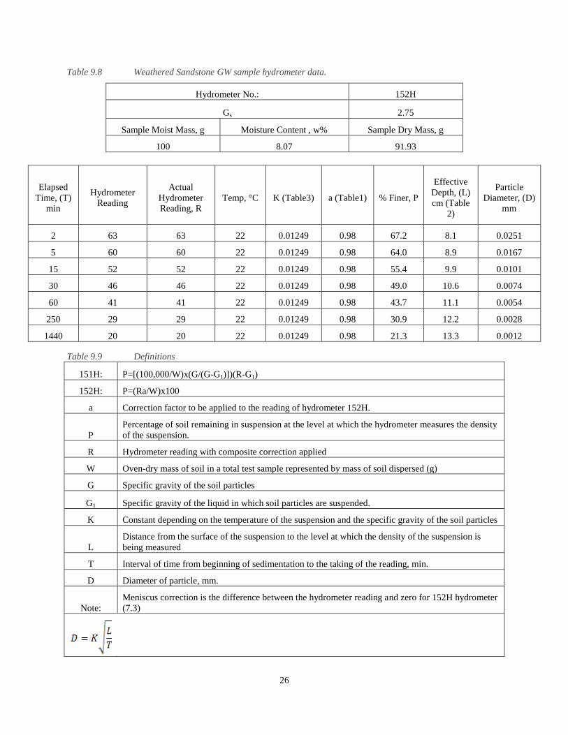
26
Table 9.8 Weathered Sandstone GW sample hydrometer data.
Hydrometer No.: 152H
Gs 2.75
Sample Moist Mass, g Moisture Content , w% Sample Dry Mass, g
100 8.07 91.93
Elapsed
Time, (T)
min
Hydrometer
Reading
Actual
Hydrometer
Reading, R
Temp, °C K (Table3) a (Table1) % Finer, P
Effective
Depth, (L)
cm (Table
2)
Particle
Diameter, (D)
mm
2 63 63 22 0.01249 0.98 67.2 8.1 0.0251
5 60 60 22 0.01249 0.98 64.0 8.9 0.0167
15 52 52 22 0.01249 0.98 55.4 9.9 0.0101
30 46 46 22 0.01249 0.98 49.0 10.6 0.0074
60 41 41 22 0.01249 0.98 43.7 11.1 0.0054
250 29 29 22 0.01249 0.98 30.9 12.2 0.0028
1440 20 20 22 0.01249 0.98 21.3 13.3 0.0012
Table 9.9 Definitions
151H: P=[(100,000/W)x(G/(G-G1)])(R-G1)
152H: P=(Ra/W)x100
a Correction factor to be applied to the reading of hydrometer 152H.
P
Percentage of soil remaining in suspension at the level at which the hydrometer measures the density
of the suspension.
R Hydrometer reading with composite correction applied
W Oven-dry mass of soil in a total test sample represented by mass of soil dispersed (g)
G Specific gravity of the soil particles
G1 Specific gravity of the liquid in which soil particles are suspended.
K Constant depending on the temperature of the suspension and the specific gravity of the soil particles
L
Distance from the surface of the suspension to the level at which the density of the suspension is
being measured
T Interval of time from beginning of sedimentation to the taking of the reading, min.
D Diameter of particle, mm.
Note:
Meniscus correction is the difference between the hydrometer reading and zero for 152H hydrometer
(7.3)

27
Figure 9.2 Grain size distribution graph including hydrometer data.

28
9.4 SPECIFIC GRAVITY – TEST 1
Specific gravity testing was performed according to ASTM standard test method D 854. Three tests were run in
order to ensure the accuracy of the data. The objective of the specific gravity testing was to obtain knowledge about
the physical characteristics of the material. For the first test, the specific gravity was found to be 2.81. For the
duplicate test, the specific gravity was found to be 2.75. The high precision of the tests is represented by the
coefficient of variation of 0.014. The results for the first test and the duplicate test are shown in the following
tables.
Table 9.10 Test results for specific gravity testing of weathered sandstone
Test Number 1 2 3
Temperature, T (oC) 22.5 22.5 22.5
Density of Water, ρw (g/ML) 0.99766 0.99766 0.99766
Temperature Coefficient, K 0.99945 0.99945 0.99945
Volume of Pycnometer, Vp (mL) 500 500 500
Wt. of Pycnometer, Mp (g) 166.15 167.96 160.61
Sample+Pycnomter+Water, Mpws,t (g) 693.76 695.76 687.47
Pycnometer+Water, Mpw,t (g) 664.35 666.04 657.59
Dry Sample Mass, Ms (g) 46.09 46.09 46.09
Wt. of Sample (g) 50.00 50.00 50.00
Specific Gravity of soil solids, Gt 2.76 2.82 2.84
Specific Gravity at Test Temp., Gtt 2.76 2.81 2.84
Table 9.11 Test statistics for specific gravity of soil solids.
Average Specific Gravity, Gt: 2.810
Sample Standard Deviation for Gt (s) 0.041
Coefficient of Variation for Gt (COV) 0.014

29
Table 9.12 Test statistics for specific gravity at the test temperature.
Avg. Specific Gravity at Test Temp, Gtt: 2.810
Sample Standard Deviation for Gtt, (s) 0.041
Coefficient of Variation for Gtt (COV) 0.014
Table 9.13 Water content for determining the dry mass of the test specimen.
Test Number 1
Empty Container, Mc, (g) 30.00
Container + Wet Sample, Mcms, (g) 86.48
Container + Dry Sample, Mcds, (g) 82.66
Moisture content w (%) 7.25
Average Moisture Content (%): 7.81
Table 9.14 Definitions
Mp = the mass of the dry pycnometer, g
Vp = the volume of the pycnometer, mL
ρw,t = the density of water at the test temperature (Tt), g/mL
ρs = the density of the soil solids (Mg/m3)
or (g/cm
3)
w = (Mw/Ms) x 100 (%)
Mpws,t = the mass of pycnometer, water, and soil solids at the test temperature, (Tt), (g)
K = temperature coefficient
Mw = mass of water = Mcms - Mcds (g)
Ms = mass of dry sample = Mcds - Mc (g)
Mpw,t = mass of the pycnometer and water at the test temperature (Tt), g
Note: K and ρw values acquired in Table 1 of ASTM D 854 -06
Mpw,t = Mp + (Vp * ρw,t)
GToC = K * Gt
Gt = ρs/ρw,t = Ms/(Mρw,t-(Mρws,t-Ms))

30
9.5 SPECIFIC GRAVITY – TEST 2
Specific gravity testing was performed according to ASTM standard test method D 854. Three tests were run in
order to ensure the accuracy of the data. The objective of the specific gravity testing was to obtain knowledge about
the physical characteristics of the material. This duplicate test was performed to achieve high precision for the
specific gravity testing of the weathered sandstone. The coefficient of variation of the data was found to be 0.002;
implying little variation in the results. The average specific gravity was found to be 2.75. The data and results for
the duplicate specific gravity test are shown in the following tables.
Table 9.15 Test results for specific gravity testing
Test Number 1 2 3
Temperature, T (oC) 22.00 22.00 22.00
Density of Water, ρw,t (g/ML) 0.99777 0.99777 0.99777
Temperature Coefficient, K 0.99957 0.99957 0.99957
Volume of Pycnometer, Vp (mL) 500.00 500.00 500.00
Wt. of Pycnometer, Mp (g) 168.09 168.29 160.72
Sample+Pycnomter+Water, Mpws,t (g) 693.51 695.3 687.21
Pycnometer+Water, Mpw,t (g) 664.23 666.06 657.92
Dry Sample Mass, Ms (g) 45.97 45.97 45.97
Wt. of Sample (g) 50.00 50.00 50.00
Specific Gravity of soil solids, Gt 2.75 2.75 2.76
Specific Gravity at Test Temp., Gtt 2.75 2.75 2.76
Table 9.16 Test statistics for specific gravity of soil solids.
Average Specific Gravity, Gt: 2.75
Sample Standard Deviation for Gt, s 0.004
Coefficient of Variation for Gt (COV) 0.002
Table 9.17 Test statistics for specific gravity at the test temperature.
Avg. Specific Gravity at Test Temp, Gtt: 2.75
Sample Standard Deviation for Gtt, (s) 0.004
Coefficient of Variation for Gtt (COV) 0.002
Table 9.18 Water content for determining the dry mass of the test specimen.
Test Number 1 2 3
Empty Container, Mc, (g) 17.41 17.3 18.77
Container + Wet Sample, Mcms, (g) 73.92 80.97 80.85
Container + Dry Sample, Mcds, (g) 69.63 76.29 76.22
Moisture content w (%) 8.22 7.93 8.06
Average Moisture Content (%): 8.07
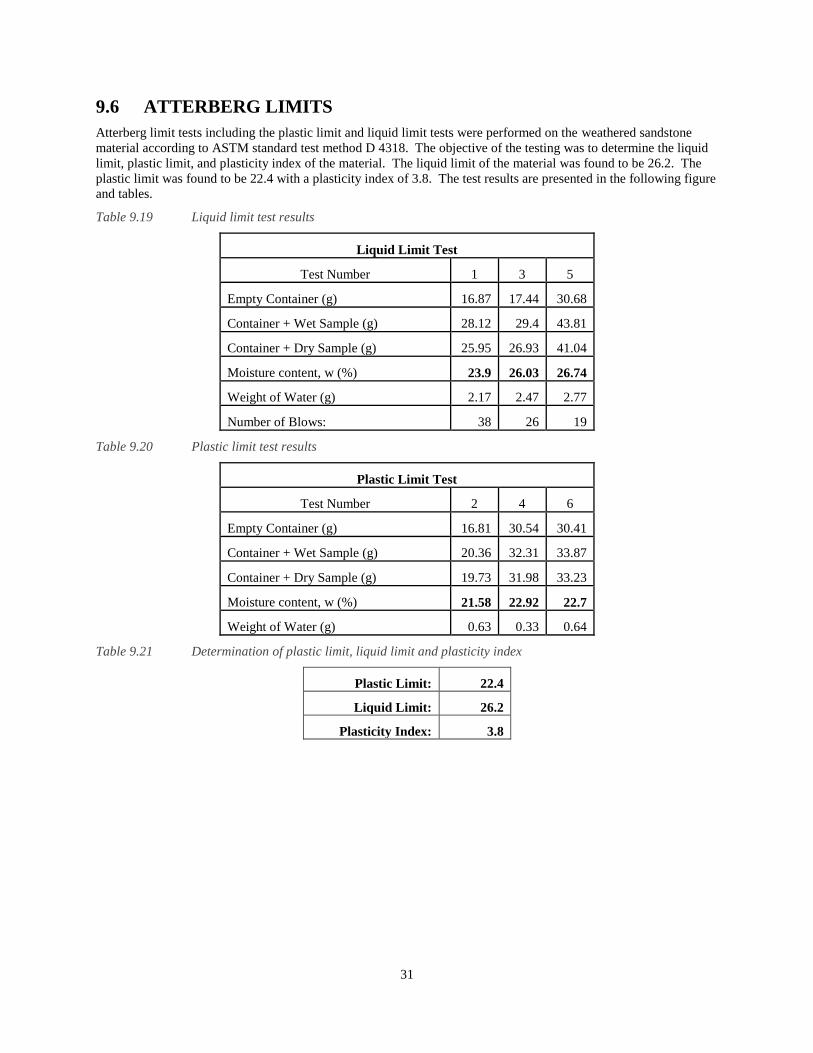
31
9.6 ATTERBERG LIMITS
Atterberg limit tests including the plastic limit and liquid limit tests were performed on the weathered sandstone
material according to ASTM standard test method D 4318. The objective of the testing was to determine the liquid
limit, plastic limit, and plasticity index of the material. The liquid limit of the material was found to be 26.2. The
plastic limit was found to be 22.4 with a plasticity index of 3.8. The test results are presented in the following figure
and tables.
Table 9.19 Liquid limit test results
Liquid Limit Test
Test Number 1 3 5
Empty Container (g) 16.87 17.44 30.68
Container + Wet Sample (g) 28.12 29.4 43.81
Container + Dry Sample (g) 25.95 26.93 41.04
Moisture content, w (%) 23.9 26.03 26.74
Weight of Water (g) 2.17 2.47 2.77
Number of Blows: 38 26 19
Table 9.20 Plastic limit test results
Plastic Limit Test
Test Number 2 4 6
Empty Container (g) 16.81 30.54 30.41
Container + Wet Sample (g) 20.36 32.31 33.87
Container + Dry Sample (g) 19.73 31.98 33.23
Moisture content, w (%) 21.58 22.92 22.7
Weight of Water (g) 0.63 0.33 0.64
Table 9.21 Determination of plastic limit, liquid limit and plasticity index
Plastic Limit: 22.4
Liquid Limit: 26.2
Plasticity Index: 3.8

32
Figure 9.3 Liquid limit graph for the weathered sandstone material

33
10. MATERIAL PROPERTIES: UNWEATHERED SANDSTONE
OVERBURDEN
10.1 SOIL CLASSIFICATION
The material under inspection in this section was classified using the United Soil Classification System (USCS) –
ASTM D 2487. After assessment, the unweathered sandstone material was classified to be a well graded sand (SW).
10.2 MOISTURE CONTENT
Testing was performed according to ASTM standard test method D 2216-05. The sampling was performed on a hot,
dry day; however, the moisture content was measured in the laboratory after the specimens acclimated to the indoor
climate. There was little variation in the results. The coefficient of variation was found to be 0.052, implying high
precision in the data. The following tables present the results for the triplicate specimen testing.
Table 10.1 Moisture Content Data
Test Number 1 2 3
Empty Container, Mc, (g) 16.89 21.79 30.03
Container + Wet Sample, Mcms, (g) 70.86 74.82 100.21
Container + Dry Sample, Mcds, (g) 69.37 73.33 98.42
Moisture content w (%) 2.84 2.89 2.62
Table 10.2 Average Moisture Content and Statistics
Average Moisture Content (%): 2.78
Sample Standard Deviation (s) 0.145
Coefficient of Variation (COV) 0.052
Table 10.3 Equations Used
Mw = mass of water = Mcms - Mcds
Ms = mass of dry sample = Mcds - Mc
w = (Mw/Ms) x 100

34
10.3 AS RECEIVED GRAIN SIZE DISTRIBUTION
Sieve analysis was performed according to ASTM D 422-63. A duplicate test was performed to ensure accuracy in
the data. The objective of this testing was to obtain appropriate data in order to classify the material, and
understand its original as received grain size distribution. The as received grain size distribution results were a
critical element in the understanding of material changes that can occur during construction under different
compaction energies. For the first test the critical indices were D90 = 12, D60 = 2.7, D50 = 1.6, D30 = 0.55, D25 =
0.40, D10 = 0.13(mm). The uniformity coefficient (Cu) was 20.77 and the coefficient of gradation (Cc) was 0.86.
For the second test the critical indices were D90 = 10.7, D60 = 3.0, D50 = 1.6, D30 = 0.55, D25 = 0.39, D10 = 0.12(mm).
The uniformity coefficient (Cu) was 25.00 and the coefficient of gradation (Cc) was 0.84. The data approximately
followed the same trend along their curves. The precision of the data is shown by a coefficient of variation for the
uniformity coefficient of 0.131, and a coefficient of variation for the coefficient of gradation of 0.018. The
hydrometere analysis illustrated that there are few fines in the sample relative to the sample size. The data is shown
in the following figures and tables.
Table 10.4 Critical Index-Values and Coefficients
Results
Critical Indices Test 1 Test 2
D90 12 10.7
D60 2.7 3
D50 1.6 1.6
D30 0.55 0.55
D25 0.4 0.39
D10 0.13 0.12
Uniformity Coefficient, Cu 20.77 25
Coefficient of Gradation, Cc 0.86 0.84
Table 10.5 Uniformity coefficient statistics
Uniformity Coefficient, Cu
Average Uniformity Coefficient 22.885
Sample Standard Deviation (s) 2.992
Coefficient of Variation (COV) 0.131

35
Table 10.6 Coefficient of gradation statistics
Coefficient of Gradation, Cc
Average Coefficient of Gradation (%) 0.851
Sample Standard Deviation (s) 0.015
Coefficient of Variation (COV) 0.018
Figure 10.1 Grain Size Distribution of two samples of unweathered sandstone overburden SW-SM.

36
Table 10.7 Unweathered Sandstone SW-SM sample hydrometer data.
Hydrometer No.: 152H
Gs 2.75
Sample
Moist
Mass, g
Moisture
Content , w%
Sample
Dry
Mass, g
100 2.78 97.22
Elapsed
Time, (T)
min
Hydrometer
Reading
Actual
Hydrometer
Reading, R
Temp,
°C
K
(Table3)
a
(Table1)
%
Finer,
P
Effective
Depth, (L)
cm (Table
2)
Particle
Diameter,
(D) mm
2 60 60 22 0.01294 0.98 60.5 6.5 0.0233
5 56 56 22 0.01294 0.98 56.4 7.1 0.0154
15 46 46 22 0.01294 0.98 46.4 8.8 0.0099
30 40 40 22 0.01294 0.98 40.3 9.7 0.0074
60 36 36 22 0.01294 0.98 36.3 10.4 0.0054
250 26 26 22 0.01294 0.98 26.2 12 0.0028
1440 18 18 22 0.01294 0.98 18.1 13.3 0.0012
Figure 10.2 Grain size distribution including hydrometer data.

37
10.4 SPECIFIC GRAVITY
Specific gravity testing was performed according to ASTM standard test method D 854. The objective of the
specific gravity testing was to obtain knowledge about the physical characteristics of the material. The specific
gravity was found to be 2.69. The precision of the testing was reflected by the coefficient of variation. The
coefficient of variation was found for the specific gravity and the specific gravity at the test temperature to be 0.029.
The test data are shown in the following tables.
Table 10.8 Test results for specific gravity testing of unweathered sandstone.
Test Number 1 2 3 4 5 6
Temperature, T (oC) 22.00 22.00 22.00 22.00 22.00 22.00
Density of Water, ρw (g/mL) 0.99777 0.99777 0.99777 0.99777 0.99777 0.99777
Temperature Coefficient, K 0.99957 0.99957 0.99957 0.99957 0.99957 0.99957
Volume of Pycnometer, Vp (mL) 500.00 500.00 500.00 500.00 500.00 500.00
Wt. of Pycnometer, Mp (g) 167.27 169.04 160.62 159.74 152.74 154.85
Sample+Pycnomter+Water, Mpws,t (g) 694.88 696.16 688.03 688.90 681.95 683.68
Pycnometer+Water, Mpw,t (g) 663.42 666.03 657.71 657.82 650.84 653.13
Dry Sample Mass, Ms (g) 48.58 48.55 48.69 49.42 49.38 49.34
Wt. of Sample (g) 50.00 50.00 50.00 50.00 50.00 50.00
Specific Gravity of soil solids, Gt 2.84 2.64 2.65 2.69 2.70 2.63
Specific Gravity at Test Temp., Gtt 2.84 2.63 2.65 2.69 2.70 2.62
Table 10.9 Test statistics for specific gravity of soil solids.
Average Specific Gravity, Gt 2.690
Sample Standard Deviation for Gt, s 0.078
Coefficient of Variation for Gt (COV) 0.029
Table 10.10 Test statistics for specific gravity at the test temperature.
Avg. Specific Gravity at Test Temp, Gtt: 2.690
Sample Standard Deviation for Gtt, s 0.078
Coefficient of Variation for Gtt (COV) 0.029
Table 10.11 Water content for determining the dry mass of the test specimen
Test Number 1 2 3 4 5 6
Empty Container, Mc, (g) 16.89 21.79 30.03 30.47 16.76 16.84
Container + Wet Sample, Mcms, (g) 70.86 74.82 100.21 159.29 87.45 90.81
Container + Dry Sample, Mcds, (g) 69.37 73.33 98.42 157.82 86.58 89.85
Moisture content w (%) 2.84 2.89 2.62 1.15 1.25 1.31
Average Moisture Content (%): 2.01

38
10.5 ATTERBERG LIMITS – TEST 1
Atterberg limit tests included the plastic limit and liquid limit test. The tests were performed on the unweathered
sandstone material according to ASTM standard test method D 4318. A duplicate test was performed in order to
ensure accuracy in the data. The objective of the testing was to determine the liquid limit, plastic limit, and
plasticity index of the material. For the first test the liquid limit of the material was found to be 19.3. The plastic
limit was found to be 16.3 with a plasticity index of 3.1 which indicates that the material is slightly plastic (PL 1-5)
(Das, 2006). For the second test the liquid limit of the material was found to be 19.1. The plastic limit was found to
be 16.5 with a plasticity index of 2.6. The test results are presented in the following figure and tables.
Table 10.12 Liquid limit test results
Liquid Limit Test
Test Number 1 5 3
Empty Container (g) 18.80 30.28 16.90
Container + Wet Sample (g) 32.55 45.46 35.71
Container + Dry Sample (g) 30.25 43.01 33.00
Moisture content, w (%) 20.09 19.25 16.83
Weight of Water (g) 2.30 2.45 2.71
Number of Blows: 16 26 39
Table 10.13 Plastic Limit Test results
Plastic Limit Test
Test Number 2 4 6
Empty Container (g) 17.4 30.46 16.9
Container + Wet Sample (g) 20.1 36.29 20.3
Container + Dry Sample (g) 19.71 35.51 19.82
Moisture content, w (%) 16.88 15.45 16.44
Weight of Water (g) 0.39 0.78 0.48
Table 10.14 Determination of plastic limit, liquid limit and plasticity index
Plastic Limit: 16.3
Liquid Limit: 19.3
Plasticity Index: 3.1

39
Figure 10.3 Liquid Limit graph for test 1
10.6 ATTERBERG LIMITS – TEST 2
Atterberg limit tests included the plastic limit and liquid limit test. The tests were performed on the unweathered
sandstone material according to ASTM standard test method D 4318. This duplicate test was performed in order to
ensure accuracy in the data. The objective of the testing was to determine the liquid limit, plastic limit, and
plasticity index of the material. For this duplicate test, the liquid limit of the material was found to be 19.1. The
plastic limit was found to be 16.5 with a plasticity index of 2.6 which indicates that the soil is slightly plastic (PL 1-
5) (Das, 2006). The test results for the Atterberg Limits are shown in the following tables and figure.
Table 10.15 Liquid limit test results
Liquid Limit Test
Test Number 1 3 5 7
Empty Container (g) 18.8 16.9 30.28 17.45
Container + Wet Sample (g) 30.65 32.69 39.02 32.05
Container + Dry Sample (g) 28.66 30.16 37.66 29.53
Moisture content w (%) 20.18 19.08 18.43 20.86
Weight of Water (g) 1.99 2.53 1.36 2.52
Number of Blows: 17 25 32 15

40
Table 10.16 Plastic limit test results
Plastic Limit Test
Test Number 2 4 6 8
Empty Container (g) 17.4 30.46 16.9 16.87
Container + Wet Sample (g) 18.82 35.48 18.44 19.61
Container + Dry Sample (g) 18.62 34.74 18.22 19.24
Moisture content w (%) 16.39 17.29 16.67 15.61
Weight of Water (g) 0.2 0.74 0.22 0.37
Table 10.17 Determination of plastic limit, liquid limit and plasticity index
Plastic Limit: 16.5
Liquid Limit: 19.1
Plasticity Index: 2.6
Figure 10.4 Liquid limit graph for test 2

41
10.7 WEATHERED AND UNWEATHERED SANDSTONE
COMPARISON
The two materials “unweathered sandstone” and “weathered sandstone” were tested for their individual geotechnical
material properties and as received grain size distributions. The results show that the materials are somewhat
different. The weathered and the unweathered sandstone are both slightly plastic soils (Das, 2006). The grain size
analysis illustrates that the gradations do vary. No strength testing was performed for the weathered material, and it
was not included in the numerical modeling of the slopes. Since most of the volume of a landform design typically
consists of overburden material, only the weathered sandstone was used for input into the numerical models. A
summary of the material properties and as received grain size distributions are shown in Figure 10.5 and Table
10.18. It is important to note that the Atterberg limits test method was for the material passing a #40 sieve. The
unweathered material was reclassified as a well graded sand with silt or SW-SM, as the more coarse particles were
separated for the laboratory testing.
Table 10.18 Soil Property summary table for unweathered and weathered sandstone
Soil Property
Summary
Unweathered
Sandstone
Weathered
Sandstone
Soil Classification SW GW
As Received Moisture
Content, w (%) 2.78 8.07
As Received GSD
Test 1
Cu (mm) 20.77 40.91
Cc (mm) 0.86 2.02
Test 2
Cu (mm) 25 23.79
Cc (mm) 0.84 1.44
Specific Gravity, Gs 2.69 2.81
Atterberg Limits – Passing #40
LL 19.3 22.4
PL 16.3 26.2
PI 3.1 3.8
Figure 10.5 As received grain size distributions of weathered and unweathered sandstone

42
11. COMPACTION
Compaction testing was performed to find the maximum dry density of the unweathered sandstone overburden
material at three predetermined compaction energies. The tests were run at a standard proctor compaction effort
(energy applied = 592.5 kJ/m3), at a 34% Proctor effort (energy applied = 203.6 kJ/m
3), and at an 11% Proctor
compaction effort (67.85 kJ/m3). Multiple water contents were used for the testing for the optimization of each test.
The objective of the compaction testing was to find the optimum and minimum dry density of the material at the
compaction energies listed above. The compaction testing data are shown in the following tables and figures.
11.1 STANDARD PROCTOR (592.5 KJ/M3)
The testing described in this section were run at a standard proctor compaction effort (energy applied = 592.5
kJ/m3). Four water contents were tested. The water contents were calculated to be 4.12%, 9.94%, 11.54%, and
12.86%. The optimum dry density of the material was found to be 18.75 kN/m3 at a water content of 10.75%. The
data are shown in the following table and figure.
Table 11.1 Compaction test results
Test Calculations Test 1 Test 2 Test 3 Test 4
Specific Gravity of Soil, Gs 2.69 2.69 2.69 2.69
Dry Unit Weight of Compacted Specimen(KN/m3), γd 16.65 18.51 18.54 13.92
Dry Unit Weight at S=1.0 (KN/m3),γd 19.57 20.09 20.78 23.71
Dry Unit Weight at S=0.9 (KN/m3),γd 19.03 19.58 20.3 23.45
Degree of Saturation (%), S=Gs*w/e 0.59 0.73 0.64 0.12
Saturated Water Content, wsat(%) 21.62 15.71 15.64 33.14
Water Content, w=(Mw/Ms)x100(%) 12.86 11.54 9.94 4.12
Figure 11.1 Standard proctor curve with lines at 100% and 90% saturation.

43
11.2 34% PROCTOR COMPACTION ENERGY: 12 BLOWS/LAYER, 2
LAYERS (203.6 KJ/M3)
The testing described in this section were run at 34% Proctor compaction effort (energy applied = 203.6 kJ/m3). The
test applied 12 blows of a 5 pound compaction hammer to 2 layers of material in a typical compaction mold. The
volume of the compaction mold is given in the data below. Seven water contents were tested. The water contents
were calculated to be 7.45%, 9.57%, 11.20%, 12.73%, 12.85%, 15.73%, and 17.97%. The optimum dry density of
the material was found to be 18.1 kN/m3 at a water content of 14.5%. The data are shown in the following table and
figure.
Table 11.2 Compaction Test Results
Test Calculations Test 1 Test 2 Test 3 Test 4 Test 5 Test 6 Test 7
Specific Gravity of Soil, Gs 2.69 2.69 2.69 2.69 2.69 2.69 2.69
Dry Unit Weight of Compacted Specimen (KN/m3), γd 16.11 16.21 16.48 17.98 17.94 17.8 14.37
Dry Unit Weight at S=1.0 (KN/m3),γd 21.94 20.95 20.24 19.57 19.62 18.51 17.75
Dry Unit Weight at S=0.9 (KN/m3),γd 21.54 20.48 19.73 19.03 19.08 17.91 17.13
Degree of Saturation (%), S=Gs*w/e 0.32 0.41 0.5 0.74 0.73 0.88 0.58
Saturated Water Content, wsat (%) 23.58 23.22 22.22 17.28 17.39 17.84 30.96
Water Content, (%) W= (Mw/Ms)x100 7.45 9.57 11.2 12.85 12.73 15.73 17.97
Figure 11.2 34% Proctor curve with lines at 100% and 90% saturation.
44
11.3 11% PROCTOR COMPACTION ENERGY: 4 BLOWS/LAYER, 2
LAYERS (67.85 KJ/M3)
The testing described in this section were run at an 11% Proctor compaction effort (energy applied = 67.85 kJ/m3).
The test applied 4 blows of a 5 pound compaction hammer to 2 layers of material in a typical compaction mold. The
volume of the compaction mold is given in the data below. Seven water contents were tested. The water contents
were calculated to be 4.36%, 9.78%, 11.60%, 11.65%, 15.47%, 16.89%, and 17.45%. The optimum dry density of
the material was found to be 17.6 kN/m3 at a water content of 16.89%. The minimum dry density was found to be
14.9 kN/m3 at a corresponding water content of 9.75%. The minimum dry density was used to find design
limitations in hydraulic conductivity. The hydraulic conductivity testing that was performed is described later in this
document. The data for the 11% Proctor compaction effort tests are shown in the following tables.
Table 11.3 Compaction Test Results
Test Calculations Test 1 Test 2 Test 3 Test 4 Test 5 Test 6 Test 7
Specific Gravity of Soil, Gs 2.69 2.69 2.69 2.69 2.69 2.69 2.69
Dry Unit Weight of Compacted Specimen (KN/m3), γd 15.39 16.9 15.2 14.93 15.07 17.6 16.55
Dry Unit Weight at S=1.0 (KN/m3),γd 23.57 18.6 20.07 20.85 20.05 18.11 17.92
Dry Unit Weight at S=0.9 (KN/m3),γd 23.3 18.01 19.55 20.38 19.53 17.5 17.31
Degree of Saturation (%), S=Gs*w/e 0.16 0.75 0.43 0.34 0.42 0.92 0.79
Saturated Water Content, wsat (%) 26.45 20.74 27.22 28.41 27.79 18.46 21.97
Water Content, (%) W= (Mw/Ms)x100 4.36 15.47 11.6 9.78 11.65 16.89 17.45
Figure 11.3 11% Proctor compaction curve with lines at 100% and 90% saturation.

45
Figure 11.4 Compaction curve compilation
11.4 DISCUSSION
The compaction curves in Figure 11.4 show different behaviors. The standard proctor curve is a typical bell shaped
curve with an optimum dry unit weight of 18.75 kN/m3 at a moisture content of approximately 10.75%. The 34%
proctor curve resembles a transition between standard proctor and 11% proctor curves. The optimum dry density of
the 34% proctor curve was 18.1 kN/m3 at a moisture content of 14.50%. The 11% proctor curve shows a
compaction curve resembling a standard behavior for a well graded sand. The optimum dry density of the 11%
proctor was at 17.6 kN/m3 with a moisture content of approximately 17.00%. The minimum dry density of the 11%
curve was at 10.50% moisture content at a value of 14.90 kN/m3. The compaction energy applied in these three
scenarios varied from 592.5 kJ/m3 (standard proctor), 203.6 kJ/m
3(
34% proctor), and 67.85 kJ/m
3 (11% proctor).
The optimum dry densities did not increase by much, only a difference of 1.15 kN/m3 between standard proctor and
11% proctor compaction. The corresponding moisture contents for these maximums varied from 10.75% (standard
proctor) to 17.00% (11% proctor) at a difference of 6.25%. The material does not need a significant amount of
compaction in order to achieve a high dry density, but it does need the accompanying moisture content to achieve it.

46
11.5 VARIABILITY IN COMPACTION
After reducing the compaction data, it was found that some significant variability occurred for the 34% and 11%
Proctor compaction effort testing. The variability is a result of a thick first lift in the compaction mold. At a low
energy, some of the specimen could not experience the full effect of the compaction effort. The points lying off of
the curve are the compaction points for 34% Proctor compaction effort permeability triplicate specimen testing and a
direct shear specimen. The variability effects are shown in the figures below.
Figure 11.5 34% Proctor compaction energy (203.6 kJ/m3): Variability in dry density
Figure 11.6 11% Proctor Compaction Energy (67.85 kJ/m3): Variability in dry density

47
12. STRENGTH TESTING
The shear strength testing was performed on a GeoJac direct shear testing device. Each test was performed at a
saturated, consolidated condition. The specimens were prepared as a standard proctor compaction sample, 34%
Proctor compaction effort sample, and an 11% Proctor compaction effort sample. The angle of internal friction ( )
was calculated using Mohr-Coulomb failure criterion concepts. The tests were performed on the gray unweathered
well graded sand with silt material to determine the shear strength properties of the material under specified normal
stress conditions. These stress conditions were determined by multiplying the optimum density of the soil by the
depth of a valley fill at the Coal MAC site in Logan, WV. The initial stresses were adjusted based on the
capabilities of the testing equipment. The maximum normal stresses and shear strains of the equipment capability
were sought to investigate thoroughly the residual strength of the material.
13. UNWEATHERED SANDSTONE OVERBURDEN
The strength testing phase was organized into three different test specimens with predetermined specified
compaction energies which each had unique void ratios. The compaction energies were at a standard proctor effort
of 592.5 kJ/m3, a 65.64% reduced compaction effort at 203.6 kJ/m
3 or 34.36% of a standard proctor effort, and an
even further reduced compaction effort at 11.45% of standard proctor equal to 67.85 kJ/m3
or 88.55% reduced.
These three compaction energies will be referred to as “34% Proctor,” “11% Proctor,” and Standard Proctor. The
specimens were prepared to target the optimum dry density for their respective compaction energies. Each
compacted specimen was extruded approximately one third the length of the compaction mold. The three layers
were captured in a direct shear specimen ring. The testing was performed on a GeoJac® direct shear testing device.
The software used to reduce the data was DigiShear™. Loading schedules were determined from analyzing a valley
fill at a surface mine in Logan, West Virginia. After the normal stress conditions were determined, they were
modified to not exceed the loading limitations of the testing devices. The tests were run at a saturated condition.
The data and results for the testing are shown in the following tables and graphs. The following two figures show
the valley fill under inspection for this testing.
Figure 13.1. Shows the centerline and the points of evaluation on the valley fill under inspection in this section.

48
Figure 13.2. Slope profile of an AOC fill design illustrating determined stress evaluation points and slope
dimensions.
Table 13.1. Stress conditions for direct shear test depths (DS1, DS2, DS3)
Compaction
Condition Test Points
Dry Density, γd
[kN/m2]
Depth, d
[m]
Normal Stress,
σ (γd*d) [kPa]
Standard
Proctor
3 18.39 0.00 0.00
2 18.39 97.02 1784.26
1 18.39 145.54 2676.40
34% Proctor
DS31 18.56 32.33 600.07
DS32 18.56 64.66 1200.14
DS33 18.56 134.72 2500.32
11% Proctor
DSL1 16.81 35.69 600.00
DSL2 16.81 71.39 1200.00
DSL3 16.81 148.72 2500.00
The depths of the stress conditions varied as a result of equipment maximum loading. The 34% proctor sample dry
density was in fact higher than the standard proctor sample. This was a function of climatic variability in the
laboratory. Moisture content varied some throughout the testing, and the target dry densities were not fully
achieved. For the standard proctor sample, the third point was made to be at the origin of the graph to demonstrate a
zero cohesion condition. The maximum normal stress and shear strain conditions were sought to investigate the
behavior of the residual strength of the unweathered sandstone. The objective of the residual strength investigation
was to give insight into slope strength.

49
13.1 STANDARD PROCTOR (592.5 KJ/M3)
A standard proctor compaction specimen was prepared and layer depths were each approximately 1/3 of the height
of the compaction mold. After compaction, the specimen was extruded from the compaction mold approximately
one third at a time. The center of each layer was captured in a direct shear ring mold. The remaining material for
each layer was used for grain size distribution analysis. Direct shearing tests were performed on each ring
specimen. The stress conditions for consolidation were found by multiplying the optimum dry density of the
crushed rock material by the depth of the valley fill profile shown below. It was determined that an additional point
could be assumed on the Mohr-Coulomb failure envelope at the origin (0 kPa, 0 kPa) since the material was
classified as a well graded sand with silt and would have little cohesion. The consolidation stress conditions were at
a normal stress of 1784.26 kPa and 2676.40 kPa. The maximum shear stresses that occurred during the testing were
1029.95 kPa, and 1342.94 kPa, respectively. For DS1, the testing equipment reached its maximum loading
capability before peak strength, but likely very near to it around a strain of approximately 7.5%. The maximum
shear stress that was read was taken to be the maximum. The testing was performed at a saturated condition. An
apparent cohesion resulted from graphing a best fit line to the data points. The apparent cohesion is understood to
be the result of the creation of a negative pore pressure in the specimen during the shearing phase of the testing. The
differences of φ’ are shown for a best fit line and where cohesion equals zero. The data and results are shown in the
following tables and figures.

50
Table 13.2. Direct shear standard proctor compaction specimen data.
Test Number DS Specimen
Assumed moisture content (%) 10.75
Mold Weight (g), Mmd 2042.22
Specimen+Mold Weight (g), Mt 3965.00
Volume of Mold (cm3),
V 940.00
Specific Gravity of Soil, Gs 2.69
Unit Weight of Water @ 20oC (KN/m
3), γw 9.79
Unit Weight of Water @ 20oC (lb/ft
3), γw 62.34
Moist Unit Weight of Compacted Specimen (g/cm3), γm 2.05
Dry Unit Weight of Compacted Specimen (g/cm3), γd 1.88
Dry Unit Weight of Compacted Specimen (KN/m3), γd 18.39
Dry Unit Weight of Compacted Specimen (lb/ft3), γd 117.11
Dry Unit Weight at S=1.0 (KN/m3),γd 21.18
Dry Unit Weight at S=0.9 (KN/m3),γd 20.73
Dry Unit Weight at S=1.0 (lb/ft3), γd 134.88
Dry Unit Weight at S=0.9 (lb/ft3), γd 132.01
Void Ratio, e=((Gs*γw)/ γd)-1 0.43
Degree of Saturation (%), S=Gs*w/e 0.56
Saturated Water Content, wsat (%) 16.06
Compaction Energy kJ/m3 (ft-lb/ft
3) 592.5 (12375)
Assumed moisture content (%) 10.75
Container Mass (g), Mc 209.89
Container+Moist Specimen Mass (g), Mcms 572.58
Intial Container+Oven Dry Specimen Mass (g), Mcds 542.50
Mass of Water (g), Mw= Mcms-Mcds 30.08
Mass of Solids (g), Ms= Mcds-Mc 332.61
Water Content, (%) W= (Mw/Ms)x100 9.04

51
Figure 13.3. Comparison of the direct shear standard proctor compaction specimen and other standard
proctor compaction data.

52
Table 13.3. Direct shear peak data and calculated values
Max Shear Stress vs. Normal Stress
Date Sample Compaction Material
7/28/2011 GrayDS1 Standard Proctor Passing No. 4
Specimen Number Max Shear Stress (ksf) Max Shear Stress(psf) Normal Stress (psf)
1 28.04 28044 55890
2 21.51 21508 37260
3 0 0 0
Specimen Number Max Shear Stress(kPa) Normal Stress (kPa)
1 1342.94 2676.40
2 1029.95 1784.26
3 0 0
m = 0.51 m = 0.53
best fit'(degrees) = 27.14 c’=0'(degrees) = 27.70
c'(psf) = 602.57 c'(kPa) = 0.00
c'(kPa) = 28.86 Figure 13.4. Shear stress versus normal stress plot of the standard proctor specimen

53
Figure 13.5. Shear stress versus normal stress saturated and unsaturated conditions of the standard proctor
specimen

54
Figure 13.6. Shear stress versus horizontal displacement of test 1 (DS1) and test 2 (DS2).
Figure 13.7. Shear stress versus shear strain of test 1 (DS1) and test 2 (DS2)
The jump on Figure 13.6 and Figure 13.7 represents a shear box set up error. The shearing pins used to separate the
top and bottom of the shearing box 0.025in were not adequately loosened. The result is the jump between the shear
stress of 200 and 400 kPa to overcome the friction caused by the pins on the shear box. The initial inconsistency of
the curves also represents this error. The friction angle that was calculated using these data are consistent with the
34% and 11% proctor strength assessment data, however, its precision up to 0.2 cm displacement is approximate as
a result of the error.

55
13.2 34% PROCTOR COMPACTION ENERGY: 12 BLOWS/LAYER, 2
LAYERS (203.6 KJ/M3)
A specimen was prepared at 34% Proctor with layer depths each approximately 1/3 of the height of the compaction
mold. After compaction, the specimen was extruded from the compaction mold approximately one third at a time.
The center of each layer was captured in a direct shear ring mold. The remaining material for each layer was used
for grain size distribution analysis. Direct shearing tests were performed on each ring specimen. The stress
conditions for consolidation were found by multiplying the optimum dry density of the crushed rock material by the
depth of the valley fill profile at the points shown below. For this test, it was determined that a forth point could be
assumed on the Mohr-Coulomb failure envelope at the origin (0 kPa, 0 kPa) since the material was classified as a
well graded sand with silt, has a low plasticity index, and therefore little cohesion. The consolidation stress
conditions were at normal stresses of 600 kPa, 1200 kPa, and 2500 kPa for the top, middle, and bottom layers,
respectively. The maximum shear stresses that occurred during the testing were 365.71 kPa, 607.73 kPa, and
1078.41 kPa, respectively. The testing was performed at a saturated condition. An apparent cohesion resulted from
graphing a best fit line to the data points. The apparent cohesion is understood to be the result of the creation of a
negative pore pressure in the specimen during the shearing phase of the testing. The differences of φ’ are shown for
a best fit line and where the cohesion equals zero. The data and results are shown in the following tables and
figures.
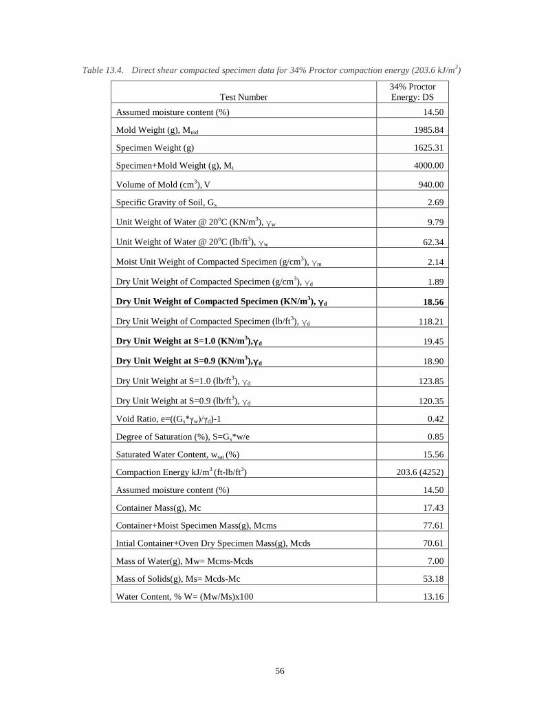
56
Table 13.4. Direct shear compacted specimen data for 34% Proctor compaction energy (203.6 kJ/m3)
Test Number
34% Proctor
Energy: DS
Assumed moisture content (%) 14.50
Mold Weight (g), Mmd 1985.84
Specimen Weight (g) 1625.31
Specimen+Mold Weight (g), Mt 4000.00
Volume of Mold (cm3),
V 940.00
Specific Gravity of Soil, Gs 2.69
Unit Weight of Water @ 20oC (KN/m
3), γw 9.79
Unit Weight of Water @ 20oC (lb/ft
3), γw 62.34
Moist Unit Weight of Compacted Specimen (g/cm3), γm 2.14
Dry Unit Weight of Compacted Specimen (g/cm3), γd 1.89
Dry Unit Weight of Compacted Specimen (KN/m3), γd 18.56
Dry Unit Weight of Compacted Specimen (lb/ft3), γd 118.21
Dry Unit Weight at S=1.0 (KN/m3),γd 19.45
Dry Unit Weight at S=0.9 (KN/m3),γd 18.90
Dry Unit Weight at S=1.0 (lb/ft3), γd 123.85
Dry Unit Weight at S=0.9 (lb/ft3), γd 120.35
Void Ratio, e=((Gs*γw)/γd)-1 0.42
Degree of Saturation (%), S=Gs*w/e 0.85
Saturated Water Content, wsat (%) 15.56
Compaction Energy kJ/m3 (ft-lb/ft
3) 203.6 (4252)
Assumed moisture content (%) 14.50
Container Mass(g), Mc 17.43
Container+Moist Specimen Mass(g), Mcms 77.61
Intial Container+Oven Dry Specimen Mass(g), Mcds 70.61
Mass of Water(g), Mw= Mcms-Mcds 7.00
Mass of Solids(g), Ms= Mcds-Mc 53.18
Water Content, % W= (Mw/Ms)x100 13.16

57
Figure 13.8. Comparison of the direct shear 34% Proctor compaction specimen and other 34% Proctor
compaction energy specimen data.

58
Table 13.5. Direct shear peak data and calculated values
Max Shear Stress vs. Normal Stress
Date Sample Compaction Material
9/26/2011 Gray M:DS31,
DS32, DS33
12 Blows/Layer, 2 Layers
(203.6 kJ/m3) Passing No. 4
Specimen Number Max Shear Stress
(ksf) Max Shear Stress(psf) Normal Stress (psf)
DS31 7.64 7637 12531
DS32 12.69 12691 25062
DS33 22.52 22520 52213
4 0 0 0
Specimen Number Max Shear
Stress(kPa) Normal Stress (kPa)
DS31 365.71 600.07
DS32 607.73 1200.14
DS33 1078.41 2500.32
4 0 0
m = 0.42 m = 0.45
φbest fit'(degrees) = 22.77 φc’=0'(degrees) = 24.36
c'(ksf) = 1287.42 c'(kPa) = 0
c'(kPa) = 61.642
Figure 13.9. Shear stress versus normal stress plot of test 1 (DS31), test 2 (DS32), and test 3 (DS33)

59
Figure 13.10. Shear stress versus normal stress saturated and unsaturated conditions of test 1 (DS31), test 2
(DS32), and test 3 (DS33)

60
Figure 13.11. Shear stress versus horizontal displacement of layer 1, layer 2, and layer 3.
Figure 13.12. Shear stress versus shear strain of layer 1, layer 2, and layer 3.

61
13.3 11% PROCTOR COMPACTION ENERGY: 4 BLOWS/LAYER, 2
LAYERS (67.85 KJ/M3)
A specimen was prepared at the minimum dry density of the 11% Proctor compaction energy compaction curve.
Layer depths were each approximately 1/3 of the height of the compaction mold. After compaction, the specimen
was extruded from the compaction mold approximately one third at a time. The center of each layer was captured in
a direct shear ring mold. The remaining material for each layer was used for grain size distribution analysis. Direct
shearing tests were performed on each ring specimen. The stress conditions for consolidation were found by
multiplying the optimum dry density of the crushed rock material by the depth of the valley fill profile at the points
shown below. For this test, it was determined that a forth point could be assumed on the Mohr-Coulomb failure
envelope at the origin (0 kPa, 0 kPa) since the material was classified as a well graded sand with silt, has a low
plasticity index, and therefore little cohesion. The consolidation stress conditions were at normal stresses of 600
kPa, 1200 kPa, and 2500 kPa for the top, middle, and bottom layers, respectively. The maximum shear stresses that
occurred during the testing were 314.19 kPa, 595.62 kPa, and 1180.03 kPa, respectively. The testing was performed
at a saturated condition. An apparent cohesion resulted from graphing a best fit line to the data points. The apparent
cohesion is understood to be the result of the creation of a negative pore pressure in the specimen during the
shearing phase of the testing. The differences of φ’ are shown for a best fit line and where the cohesion equals zero.
The data and results are shown in the following tables and figures.

62
Table 13.6. Direct shear compacted specimen data for 11% Proctor compaction energy (203.6 kJ/m3)
Test Number
11% Proctor
DS
Assumed moisture content (%) 10.50
Mold Weight (g), Mmd 1988.11
Specimen Weight (g) 1611.89
Specimen+Mold Weight (g), Mt 3600.00
Volume of Mold (cm3),
V 940.00
Specific Gravity of Soil, Gs 2.69
Unit Weight of Water @ 20oC (KN/m
3), γw 9.79
Unit Weight of Water @ 20oC (lb/ft
3), γw 62.34
Moist Unit Weight of Compacted Specimen (g/cm3), γm 1.71
Dry Unit Weight of Compacted Specimen (g/cm3), γd 1.71
Dry Unit Weight of Compacted Specimen (KN/m3), γd 16.81
Dry Unit Weight of Compacted Specimen (lb/ft3), γd 107.05
Dry Unit Weight at S=1.0 (KN/m3),γd 26.34
Dry Unit Weight at S=0.9 (KN/m3),γd 26.34
Dry Unit Weight at S=1.0 (lb/ft3), γd 167.70
Dry Unit Weight at S=0.9 (lb/ft3), γd 167.70
Void Ratio, e=((Gs*γw)/γd)-1 0.57
Degree of Saturation (%), S=Gs*w/e 0.00
Saturated Water Content, wsat (%) 21.06
Compaction Energy kJ/m3 (ft-lb/ft
3) 67.85 (1417)
Assumed moisture content (%) 10.50
Container Mass(g), Mc 30.44
Container+Moist Specimen Mass(g), Mcms 127.07
Intial Container+Oven Dry Specimen Mass(g), Mcds 118.27
Mass of Water(g), Mw= Mcms-Mcds 8.80
Mass of Solids(g), Ms= Mcds-Mc 87.83
Water Content, % W= (Mw/Ms)x100 10.02
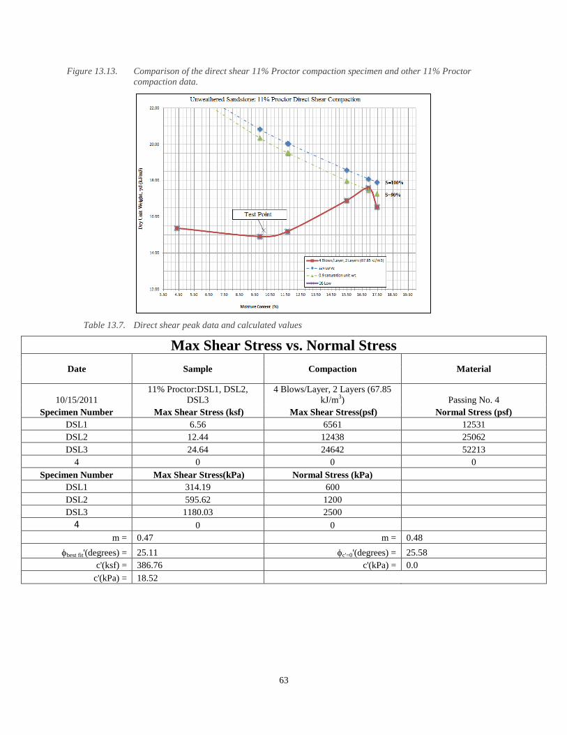
63
Figure 13.13. Comparison of the direct shear 11% Proctor compaction specimen and other 11% Proctor
compaction data.
Table 13.7. Direct shear peak data and calculated values
Max Shear Stress vs. Normal Stress
Date Sample Compaction Material
10/15/2011
11% Proctor:DSL1, DSL2,
DSL3
4 Blows/Layer, 2 Layers (67.85
kJ/m3) Passing No. 4
Specimen Number Max Shear Stress (ksf) Max Shear Stress(psf) Normal Stress (psf)
DSL1 6.56 6561 12531
DSL2 12.44 12438 25062
DSL3 24.64 24642 52213
4 0 0 0
Specimen Number Max Shear Stress(kPa) Normal Stress (kPa)
DSL1 314.19 600
DSL2 595.62 1200
DSL3 1180.03 2500
4 0 0
m = 0.47 m = 0.48
best fit'(degrees) = 25.11 c'=0'(degrees) = 25.58
c'(ksf) = 386.76 c'(kPa) = 0.0
c'(kPa) = 18.52

64
Figure 13.14. Shear stress versus normal stress plot of 11% Proctor compaction layer 1, layer 2, and layer 3
Figure 13.15. Shear stress versus normal stress saturated and unsaturated conditions of test 1 (DSL1), test 2
(DSL2), and test 3 (DSL3)

65
Figure 13.16. Shear stress versus horizontal displacement of layer 1, layer 2, and layer 3.
Figure 13.17. Shear stress versus shear strain

66
13.4 STRENGTH TESTING RESULTS
The results of the strength testing performed in sections 8.1-8.3 were useful to determine the input parameter “φ”
into GeoStudio™. The friction angle results are shown in the table below.
Table 13.8. Friction angle results with shear stresses and normal stresses shown
Compaction
Condition
Test
Points
Normal Stress,
σ (γd*d) [kPa]
Shear Stress,
τ [kPa]
Friction Angle, φ
(Best fit)
Friction Angle, φ
(zero cohesion)
Standard
Proctor
3 0.00 0.00
27.14o 27.70
o 2 1784.26 1029.95
1 2676.40 1342.94
34% Proctor
DS31 600.07 365.71
22.77o 24.36
o DS32 1200.14 607.73
DS33 2500.32 1078.41
11% Proctor
DSL1 600.00 314.19
25.11o 25.58
o DSL2 1200.00 595.62
DSL3 2500.00 1180.03
The target shear strain for each sample was 20%. The shear strain curves revealed that much of the residual strength
is retained within the sample. The reason the samples retained their strength is likely a result of the creation of the
unweathered material. The geometry of the particles of the sample is angular. The material was blasted,
unweathered rock. The angular nature of the material increases the friction between shear planes and resists
displacement. This insight is beneficial when considering slope stability. Slopes constructed with this material
should be strong and resistant to failure (FS<1).

67
14. PRE-PERMEABILITY GRAIN SIZE DISTRIBUTION
The compacted specimens were tested using standard proctor compaction energy (592.5 kJ/m3), 34% Proctor
compaction energy (203.6 kJ/m3), and an 11% Proctor compaction energy (67.85 kJ/m
3). Sieve analysis was
performed on the compacted specimens for the remainder of each of three layers from which the direct shear
specimens were taken. The objective of the testing was to determine the volume of created fines in the three layers
due to the compaction effort, and compare their distribution within the mold with the distribution of fines in the
post-permeability specimens. The desired outcome was to understand the creation, movement, and variability of
fine particles in the specimens at a pre-permeability condition and later compare the results to a post-permeability
condition grain size distribution analysis. The concept is that the testing will emulate field compaction energies and
fine particle creation. Therefore, it will be possible to understand how to construct a valley fill in order to reduce the
creation and movement of fine particles to prevent suffusion and internal erosion and ultimately increase the
durability and prolong the lifetime of the structure. The results of the testing are shown below.
14.1 GRAIN SIZE DISTRIBUTION: STANDARD PROCTOR (592.5
KJ/M3)
Grain size distribution testing was performed on three layers of a specimen that was prepared via standard proctor
compaction. The specimen was used for direct shear testing, but the remainder of the soil per layer was used for
grain size distribution testing. The third layer of the specimen could not be tested with our direct shear equipment
because the second layer maxed out the load actuators on the GeoJac equipment. The normal stresses were intended
to increase from the top layer to the bottom layer. Regardless, the grain size distribution analysis testing was
performed on the third layer of the specimen. The layers varied very little in their gradations, as shown by the
coefficient of variability for the uniformity coefficient at 0.068, and the coefficient of variation for the coefficient of
gradation at 0.116. The specimen was oven dried prior to testing. The data are shown in the following figures and
tables.
Table 14.1 Critical index values for the direct shear grain size distribution testing.
Results
Critical Indices Layer 1 Layer 2 Layer 3
D90 3.75 3.30 3.80
D60 1.65 1.05 1.80
D50 1.15 0.69 1.35
D30 0.48 0.35 0.55
D25 0.40 0.29 0.44
D10 0.15 0.10 0.15
Uniformity Coefficient, Cu 11.00 10.50 12.00
Coefficient of Gradation, Cc 0.93 1.17 1.12
Table 14.2 Uniformity coefficient statistics
Uniformity Coefficient, Cu
Average Uniformity Coefficient 11.167
Sample Standard Deviation (s) 0.764
Coefficient of Variation (COV) 0.068

68
Table 14.3 Coefficient of gradation statistics
Coefficient of Gradation, Cc
Average Coefficient of Gradation 1.073
Sample Standard Deviation (s) 0.125
Coefficient of Variation (COV) 0.116
Figure 14.1 Grain size distribution of layer 1, layer 2, layer 3.

69
14.1 GRAIN SIZE DISTRIBUTION: 34% PROCTOR COMPACTION
ENERGY (203.6 KJ/M3)
Grain size distribution testing was performed on a 34% Proctor specimen that was prepared for direct shear testing.
The remainder of the soil for the 3 layers from which direct shear ring specimens were taken was used for the grain
size distribution testing. The material was oven dried before testing. The three layers showed very little variability.
The variability is shown by the coefficient of variability for the uniformity coefficient at 0.117, and a coefficient of
variability for the coefficient of gradation at 0.048. The data are shown in the following tables and figure.
Table 14.4 Critical index values for the direct shear grain size distribution testing.
Results Layer 1 Layer 2 Layer 3
D90 3.80 3.80 3.80
D60 1.80 1.70 1.70
D50 1.40 1.30 1.30
D30 0.69 0.58 0.56
D25 0.56 0.45 0.44
D15 0.28 0.22 0.24
D10 0.17 0.13 0.13
Uniformity Coefficient, Cu 10.59 13.08 13.08
Coefficient of Gradation, Cc 1.56 1.52 1.42
Table 14.5 Uniformity coefficient statistics
Uniformity Coefficient, Cu
Average Uniformity Coefficient 12.247
Sample Standard Deviation (s) 1.437
Coefficient of Variation (COV) 0.117
Table 14.6 Coefficient of gradation statistics
Coefficient of Gradation, Cc
Average Coefficient of Gradation 1.499
Sample Standard Deviation (s) 0.071
Coefficient of Variation (COV) 0.048

70
Figure 14.2 Grain size distribution of 34% Proctor compaction effort: layer 1 (test1), layer 2 (test 2), layer 3
(test 3)

71
14.2 GRAIN SIZE DISTRIBUTION: 11% PROCTOR COMPACTION
ENERGY (67.85 KJ/M3)
Grain size distribution testing was performed on an 11% Proctor compaction energy specimen that was prepared for
direct shear testing. The remainder of the soil for the 3 layers from which direct shear ring specimens were taken
was used for the grain size distribution testing. The material was oven dried before testing. There was little
variability in the data. The variability is expressed by the coefficient of variability. The coefficient of variability for
the uniformity coefficient was 0.123. The coefficient of variability for the coefficient of gradation was 0.170. The
data are shown in the following tables and figure.
Table 14.7 Critical index values for the direct shear grain size distribution testing.
Results Layer 1 Layer 2 Layer 3
D90 4.10 4.00 4.00
D60 2.70 2.60 2.40
D50 2.20 2.00 1.80
D30 1.20 0.98 0.90
D25 0.88 0.75 0.73
D15 0.51 0.39 0.41
D10 0.28 0.22 0.25
Uniformity Coefficient, Cu 9.64 11.82 9.60
Coefficient of Gradation, Cc 1.90 1.68 1.35
Table 14.8 Uniformity coefficient statistics
Uniformity Coefficient, Cu
Average Uniformity Coefficient 10.354
Sample Standard Deviation (s) 1.268
Coefficient of Variation (COV) 0.123
Table 14.9 Coefficient of gradation statistics
Coefficient of Gradation, Cc
Average Coefficient of Gradation 1.645
Sample Standard Deviation (s) 0.279
Coefficient of Variation (COV) 0.170

72
Figure 14.3 Grain size distribution of 11% Proctor compaction effort: layer 1, layer 2, layer 3

73
15. HYDRAULIC CONDUCTIVITY
Hydraulic conductivity testing was performed using the ASTM standard test method D 5856. The target compaction
density was the maximum dry density of the unweathered sandstone overburden for the standard proctor compaction
specimen, and the 34% Proctor compaction specimen. The 11% Proctor compaction energy specimen was prepared
for the minimum dry density to establish an upper limit for the hydraulic conductivity. The objective of the
hydraulic conductivity testing was to determine the permeability of water through a test specimen at the maximum
and minimum dry density of the material. Grain size distribution tests were performed on three approximately equal
layers of the specimen after a gradient of i=100 for the standard proctor specimens, and a hydraulic gradient of i=15
for the 34% and 11% proctor specimens was permeated through each specimen for an adequate period of time, and
the hydraulic conductivity had been determined. The high gradients were chosen to accelerate the testing process.
The gradient of 100 was used on the standard proctor specimen as no hydraulic consolidation was expected, nor did
it occur. The hydraulic gradient of 15 was chosen for the reduced proctor specimens to avoid hydraulic
consolidation and accelerate the testing process as a low hydraulic conductivity was expected for the well graded
sand with silt. The purpose of the grain size distribution testing was to track the movement of material particles,
particularly the smaller diameter particles. The effort was meant to emulate field conditions replicating suffusion
phenomena and internal erosion within an AOC valley fill. The results of the testing are shown in the following
tables and figures.
15.1 HYDRAULIC CONDUCTIVITY: STANDARD PROCTOR (592.5
KJ/M3)
Hydraulic conductivity testing was performed on a standard proctor compaction effort (592.5 kJ/m3) standard
proctor specimen. The target dry density was at optimum for the standard proctor compaction effort test data. The
optimum dry density for the standard proctor compaction effort specimen was 18.75 kN/m3. Triplicate testing was
performed to ensure accuracy. The dry densities for tests 1, 2, and 3 were 18.14 kN/m3, 18.15 kN/m
3, and 18.30
kN/m3 respectively. The objective of the testing was to determine the hydraulic conductivity in order to better
understand the rate at which water would permeate through the material under inspection. The purpose of the
testing was to determine the fine particle movement within the specimen under the influence of a hydraulic gradient
i=100. After the hydraulic conductivity readings reached equilibrium, the hydraulic conductivity was determined
and the specimen was extruded approximately one third at a time. The hydraulic conductivity was determined after
the data had become stable. In these cases, the average of the last five data points was taken to be the hydraulic
conductivity of the specimens. The layers were saved and oven dried. Grain size analysis was run on three layers of
each specimen. The hydraulic conductivity data for the standard proctor compaction energy specimen are presented
in the following tables and figures. The hydraulic conductivity data is presented in Appendix I.

74
Table 15.1 Hydraulic conductivity standard proctor compaction energy specimen data.
Test Number Test 1 Test 2 Test 3
Assumed moisture content (%) 10.75 10.75 10.75
Mold Weight (g), Mmd 614.90 616.62 618.11
Specimen+Mold Weight (g), Mt 2454.57 2318.32 2416.29
Volume of Mold (cm3), V 888.52 837.04 888.52
Specific Gravity of Soil, Gs 2.69 2.69 2.69
Unit Weight of Water @ 20oC(KN/m
3), ?w 9.79 9.79 9.79
Unit Weight of Water @ 20oC(lb/ft
3), γw 62.34 62.34 62.34
Moist Unit Weight of Compacted Specimen (g/cm3), γm 2.07 2.03 2.02
Dry Unit Weight of Compacted Specimen (g/cm3), γd 1.85 1.85 1.87
Dry Unit Weight of Compacted Specimen (KN/m3), γd 18.14 18.15 18.30
Dry Unit Weight of Compacted Specimen (lb/ft3), γd 115.49 115.55 116.52
Dry Unit Weight at S=1.0 (KN/m3),γd 19.94 20.82 21.47
Dry Unit Weight at S=0.9 (KN/m3),γd 19.42 20.35 21.03
Dry Unit Weight at S=1.0 (lb/ft3), γd 126.98 132.59 136.70
Dry Unit Weight at S=0.9 (lb/ft3), γd 123.65 129.57 133.95
Void Ratio, e=((Gs*γw)/γd)-1 0.45 0.45 0.44
Degree of Saturation (%), S=Gs*(w/e) 0.71 0.59 0.52
Saturated Water Content, wsat (%) 16.80 16.78 16.33
Assumed moisture content (%) 10.75 10.75 10.75
Container Mass (g), Mc 30.40 30.55 30.52
Container+Moist Specimen Mass (g), Mcms 70.12 58.00 69.62
Intial Container+Oven Dry Specimen Mass (g), Mcds 65.89 55.54 66.58
Mass of Water (g), Mw= Mcms-Mcds 4.23 2.46 3.04
Mass of Solids (g), Ms= Mcds-Mc 35.49 24.99 36.06
Water Content, (%) W= (Mw/Ms)x100 11.92 9.84 8.43
Compaction Energy kJ/m3 (ft-lb/ft
3) 592.50 (12375)

75
Figure 15.1 Comparison of the hydraulic conductivity standard proctor compaction energy specimen and
other standard proctor compaction energy compaction data.
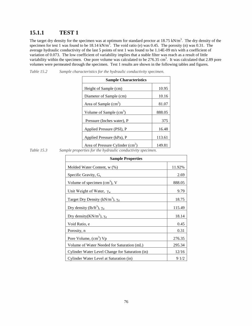
76
15.1.1 TEST 1
The target dry density for the specimen was at optimum for standard proctor at 18.75 kN/m3. The dry density of the
specimen for test 1 was found to be 18.14 kN/m3. The void ratio (e) was 0.45. The porosity (n) was 0.31. The
average hydraulic conductivity of the last 5 points of test 1 was found to be 1.14E-09 m/s with a coefficient of
variation of 0.073. The low coefficient of variability implies that a stable filter was reach as a result of little
variability within the specimen. One pore volume was calculated to be 276.35 cm3. It was calculated that 2.89 pore
volumes were permeated through the specimen. Test 1 results are shown in the following tables and figures.
Table 15.2 Sample characteristics for the hydraulic conductivity specimen.
Sample Characteristics
Height of Sample (cm) 10.95
Diameter of Sample (cm) 10.16
Area of Sample (cm2) 81.07
Volume of Sample (cm3) 888.05
Pressure (Inches water), P 375
Applied Pressure (PSI), P 16.48
Applied Pressure (kPa), P 113.61
Area of Pressure Cylinder (cm2) 149.81
Table 15.3 Sample properties for the hydraulic conductivity specimen.
Sample Properties
Molded Water Content, w (%) 11.92%
Specific Gravity, Gs 2.69
Volume of specimen (cm3), V 888.05
Unit Weight of Water, γw 9.79
Target Dry Density (kN/m3), γd 18.75
Dry density (lb/ft3), γd 115.49
Dry density(KN/m3), γd 18.14
Void Ratio, e 0.45
Porosity, n 0.31
Pore Volume, (cm3) Vp 276.35
Volume of Water Needed for Saturation (mL) 295.34
Cylinder Water Level Change for Saturation (in) 12/16
Cylinder Water Level at Saturation (in) 9 1/2

77
Table 15.4 Sample preparation information
Sample Preparation
Sample used for compaction Passing No. 4 Sieve
Density used for Compaction (% target γd) 97%
Corresponding Water Content 11.92% (Dry Side)
Table 15.5 Hydraulic gradient calculation information
Pressure calculation for a predetermined hydraulic gradient
L (ft) i γw (lb/ft3) u (psf) u (psi) u (kPa) γw (kN/m
3)
0.38 100 62.4 2372.5 16.48 113.61 9.79
Table 15.6 Definitions
Definitions:
i = h/L: Hydraulic gradient (unitless)
h = u/γw : Pressure head according to Bernoulli's equation
u = Pressure (psi)
γw= 62.4 lb/ft3 = 9.79 kN/m
3 : Unit weight of water
L = Length of specimen (height of cylinder) (cm or in)
Table 15.7 Hydraulic conductivity results – Statistics (Last 5 data points)
k Results: Last 5 Points
Average Hydraulic Conductivity (m/s) 1.14E-09
Sample Standard Deviation (s) 8.33E-11
Coefficient of Variation (COV) 0.073

78
15.1.2 TEST 2
The target dry density for the specimen was at optimum for standard proctor at 18.75 kN/m3. The dry density of the
specimen for test 2 was found to be 18.15 kN/m3. The void ratio (e) was 0.45. The porosity (n) was 0.31. The
average hydraulic conductivity of the last 5 points of test 2 was found to be 5.81E-10 m/s with a coefficient of
variation of 0.243. The low coefficient of variability implies that a stable filter was reach as a result of little
variability within the specimen. One pore volume was calculated to be 260.01 cm3. It was calculated that 3.69 pore
volumes were permeated through the specimen. Test 2 results are shown in the following tables and figures.
Table 15.8 Sample characteristics for the hydraulic conductivity specimen.
Sample Characteristics
Height of Sample (cm) 10.32
Diameter of Sample (cm) 10.16
Area of Sample (cm2) 81.07
Volume of Sample (cm3) 836.57
Pressure (Inches water), P 375
Applied Pressure (PSI), P 16.48
Applied Pressure (kPa), P 113.61
Area of Pressure Cylinder (cm2) 149.81
Table 15.9 Sample properties for the hydraulic conductivity specimen.
Sample Properties
Molded Water Content, w (%) 11.92%
Specific Gravity, Gs 2.69
Volume of specimen (cm3), V 836.57
Unit Weight of Water, γw 9.79
Target Dry Density (kN/m3), γd 18.75
Dry density (lb/ft3), γd 115.55
Dry density(KN/m3), γd 18.15
Void Ratio, e 0.45
Porosity, n 0.31
Pore Volume, (cm3) Vp 260.01
Volume of Water Needed for Saturation (mL) 277.55
Cylinder Water Level Change for Saturation (in) 12/16
Cylinder Water Level at Saturation (in) 10 1/4

79
Table 15.10 Sample preparation information
Sample Preparation
Sample used for compaction Passing No. 4 Sieve
Density used for Compaction (% target γd) 97%
Corresponding Water Content 9.84% (Dry Side)
Table 15.11 Hydraulic gradient calculation information
Pressure calculation for a predetermined hydraulic gradient
L (ft) i γw (lb/ft3) u (psf) u (psi) u (kPa) γw (kN/m
3)
0.38 100 62.4 2372.5 16.48 113.61 9.79
Table 15.12 Hydraulic conductivity results – Statistics (Last 5 data points)
k Results: Last 5 Points
Average Hydraulic Conductivity (m/s) 5.81E-10
Sample Standard Deviation (s) 1.41E-10
Coefficient of Variation (COV) 0.243

80
15.1.3 TEST 3
The target dry density for the specimen was at optimum for standard proctor at 18.75 kN/m3. The dry density of the
specimen for test 3 was found to be 18.30 kN/m3. The void ratio (e) was 0.44. The porosity (n) was 0.31. The
average hydraulic conductivity of the last 5 points of test 3 was found to be 1.82E-09 m/s with a coefficient of
variation of 0.062. The low coefficient of variability implies that a stable filter was reach as a result of little
variability within the specimen. One pore volume was calculated to be 270.95 cm3. It was calculated that 18.46
pore volumes were permeated through the specimen. Test 3 results are shown in the following tables and figures.
Table 15.13 Sample characteristics for the hydraulic conductivity specimen.
Sample Characteristics
Height of Sample (cm) 10.95
Diameter of Sample (cm) 10.16
Area of Sample (cm2) 81.07
Volume of Sample (cm3) 888.05
Pressure (Inches water), P 375
Applied Pressure (PSI), P 16.48
Applied Pressure (kPa), P 113.61
Area of Pressure Cylinder (cm2) 149.81
Table 15.14 Sample properties for the hydraulic conductivity specimen.
Sample Properties
Molded Water Content, w (%) 8.43%
Specific Gravity, Gs 2.69
Volume of specimen (cm3), V 888.05
Unit Weight of Water, γw 9.79
Target Dry Density (kN/m3), γd 18.75
Dry density (lb/ft3), γd 115.55
Dry density(KN/m3), γd 18.3
Void Ratio, e 0.44
Porosity, n 0.31
Pore Volume, (cm3) Vp 270.95
Volume of Water Needed for Saturation (mL) 315.06
Cylinder Water Level Change for Saturation (in) 13/16
Cylinder Water Level at Saturation (in) 16

81
Table 15.15 Sample preparation information
Sample Preparation
Sample used for compaction Passing No. 4 Sieve
Density used for Compaction (% target γd) 98%
Corresponding Water Content 8.43% (Dry Side)
Table 15.16 Hydraulic gradient calculation information
Pressure calculation for a predetermined hydraulic gradient
L (ft) i γw (lb/ft3) u (psf) u (psi) u (kPa) γw (kN/m
3)
0.38 100 62.4 2372.5 16.48 113.61 9.79
Table 15.17 Hydraulic conductivity results – Statistics (Last 5 data points)
k Results: Last 5 Points
Average Hydraulic Conductivity (m/s) 1.82E-09
Sample Standard Deviation (s) 1.13E-10
Coefficient of Variation (COV) 0.062
Figure 15.2 Hydraulic conductivity (k) versus time.

82
Figure 15.3 Hydraulic conductivity (k) versus pore volumes (pV).
Table 15.18 Summary values for tests 1, 2, and 3.
i γstd. proctor (kN/m3) γoptimum (kN/m
3) e n k (m/s) s (for k) COV
Test 1 100 18.14 18.75 0.45 0.31 1.14E-09 8.33E-11 0.073
Test 2 100 18.15 18.75 0.45 0.31 5.81E-10 1.41E-10 0.243
Test 3 100 18.30 18.75 0.44 0.31 1.82E-09 1.13E-10 0.062
Average -- 18.20 -- 0.45 0.31 1.18E-09 1.12E-10 0.126

83
15.2 HYDRAULIC CONDUCTIVITY: 34% PROCTOR (203.6KJ/M3)
Hydraulic conductivity testing was performed on a 34% Proctor compaction effort (203.6 kJ/m3) specimen. The
target dry density was at optimum for this compaction effort test data. The optimum dry density for the specimen
was 18.1 kN/m3. Triplicate testing was performed to ensure accuracy. The dry densities for tests 1, 2, and 3 were
16.32 kN/m3, 16.44 kN/m
3, and 17.61 kN/m
3 respectively. The objective of the testing was to determine the
hydraulic conductivity in order to better understand the rate at which water would permeate through the material
under inspection. The purpose of the testing was to determine the fine particle movement within the specimen under
the influence of a hydraulic gradient i=15. The hydraulic gradient of 15 was chosen for the 34% proctor specimens
to avoid hydraulic consolidation and accelerate the testing process as a low hydraulic conductivity was expected for
the well graded sand with silt. After the hydraulic conductivity readings reached equilibrium, the hydraulic
conductivity was determined and the specimen was extruded approximately one third at a time. The hydraulic
conductivity was determined after the data had become stable. In these cases, the average of the last five data points
was taken to be the hydraulic conductivity of the specimens. The layers were saved and oven dried. Grain size
analysis was run on three layers of each specimen. The hydraulic conductivity results are presented in the following
tables and figures. The hydraulic conductivity data is presented in Appendix I.

84
Table 15.19 Hydraulic conductivity 34% Proctor compaction energy specimen data.
Test Number Test 1 Test 2 Test 3
Assumed moisture content (%) 14.50 14.50 14.50
Mold Weight (g), Mmd 613.79 615.98 617.20
Specimen Weight (g) 1778.08 1803.46 1917.10
Specimen+Mold Weight (g), Mt 2391.87 2419.44 2534.30
Volume of Mold (cm3),
V 940.00 940.00 940.00
Specific Gravity of Soil, Gs 2.69 2.69 2.69
Unit Weight of Water @ 20oC (KN/m
3), γw 9.79 9.79 9.79
Unit Weight of Water @ 20oC (lb/ft
3), γw 62.34 62.34 62.34
Moist Unit Weight of Compacted Specimen (g/cm3), γm 1.89 1.92 2.04
Dry Unit Weight of Compacted Specimen (g/cm3), γd 1.66 1.67 1.79
Dry Unit Weight of Compacted Specimen (KN/m3), γd 16.32 16.42 17.58
Dry Unit Weight of Compacted Specimen (lb/ft3), γd 103.93 104.57 111.93
Dry Unit Weight at S=1.0 (KN/m3),γd 19.27 18.93 19.22
Dry Unit Weight at S=0.9 (KN/m3),γd 18.71 18.36 18.66
Dry Unit Weight at S=1.0 (lb/ft3), γd 122.71 120.53 122.40
Dry Unit Weight at S=0.9 (lb/ft3), γd 119.16 116.88 118.83
Void Ratio, e=((Gs*γw)/γd)-1 0.61 0.60 0.50
Degree of Saturation (%), S=Gs*w/e 0.60 0.65 0.74
Saturated Water Content, wsat (%) 22.81 22.44 18.52
Assumed moisture content (%) 14.50 14.50 14.50
Container Mass (g), Mc 18.85 22.01 17.40
Container+Moist Specimen Mass(g), Mcms 66.63 83.67 74.62
Intial Container+Oven Dry Specimen Mass(g), Mcds 60.90 75.84 67.70
Mass of Water (g), Mw= Mcms-Mcds 5.73 7.83 6.92
Mass of Solids (g), Ms= Mcds-Mc 42.05 53.83 50.3
Water Content, % W= (Mw/Ms)x100 13.63 14.55 13.76
Compaction Energy kJ/m3 (ft-lb/ft
3) 67.85 (4252)
Compaction Test
34% Proctor Compaction Energy: 12
Blows/Layer; 2 Layers

85
Figure 15.4 Comparison of the hydraulic conductivity 34% Proctor compaction energy specimen and other
34% Proctor specimen compaction data.

86
15.2.1 TEST 1
The target dry density for the specimen was at optimum for 34% proctor at 18.1 kN/m3. The dry density of the
specimen for test 1 was found to be 16.32 kN/m3. The void ratio (e) was 0.61. The porosity (n) was 0.38. The
average hydraulic conductivity of the last 5 points of test 1 was found to be 2.02E-09 m/s with a coefficient of
variation of 0.09. The low coefficient of variability implies that a stable filter was reach as a result of little
variability within the specimen. The statistics are also shown for all of the test data to illustrate that the sample
became a stable filter near the end of permeation. One pore volume was calculated to be 357.24 cm3. It was
calculated that 1.79 pore volumes were permeated through the specimen. Test 1 results are shown in the following
tables and figures.
Table 15.20 Sample characteristics for the hydraulic conductivity specimen.
Sample Characteristics
Height of Sample (cm) 11.59
Diameter of Sample (cm) 10.16
Area of Sample (cm2) 81.07
Volume of Sample (cm3) 939.54
Pressure (Inches water), P 0.00
Applied Pressure (PSI), P 2.37
Applied Pressure (kPa), P 0.11
Table 15.21 Sample properties for the hydraulic conductivity specimen.
Sample Properties
Molded Water Content, w (%) 0.14
Specific Gravity, Gs 2.69
Volume of specimen (cm3), V 939.54
Unit Weight of Water, γw 9.79
Dry density (lb/ft3), γd 103.93
Dry density (kN/m3), γd 16.32
Void Ratio, e 0.61
Porosity, n 0.38
Pore Volume, (cm3) Vp 357.24
Table 15.22 Sample preparation information
Sample Preparation
Sample used for compaction Passing No. 4 Sieve
Density used for Compaction 90% max γd
Corresponding Water Content 13.63%(Dry Side)

87
Table 15.23 Hydraulic gradient calculation information
Pressure calculation for a predetermined hydraulic gradient
L (ft) i γw (lb/ft3) u (psf) u (psi) u (kPa) γw (kN/m
3)
0.38 15.00 62.40 355.88 2.47 17.04 9.79
Table 15.24 Definitions
Definitions:
i = h/L: Hydraulic gradient (unitless)
h = u/γw : Pressure head according to Bernoulli's equation
u = Pressure (psi)
γw= 62.4 lb/ft3 = 9.79 kN/m
3 : Unit weight of water
L = Length of specimen (height of cylinder) (cm or in)
Table 15.25 Hydraulic conductivity results – Statistics (All test 1 data)
Average Hydraulic Conductivity (m/s): 9.60E-08
Sample Standard Deviation (s) 4.92E-07
Coefficient of Variation (COV) 5.12
Table 15.26 Hydraulic conductivity results – Statistics (Last 5 data points)
Last 5 Points
Average Hydraulic Conductivity (m/s): 2.02E-09
Sample Standard Deviation (s) 1.84E-10
Coefficient of Variation (COV) 0.09

88
15.2.2 TEST 2
The target dry density for the specimen was at optimum for 34% proctor at 18.1 kN/m3. The dry density of the
specimen for test 2 was found to be 16.32 kN/m3. The void ratio (e) was 0.60. The porosity (n) was 0.38. The
average hydraulic conductivity of the last 5 points of test 2 was found to be 1.69E-09 m/s with a coefficient of
variation of 0.21. The low coefficient of variability implies that a stable filter was reach as a result of little
variability within the specimen. The statistics are also shown for all of the test data to illustrate that the sample
became a stable filter near the end of permeation. One pore volume was calculated to be 352.96 cm3. It was
calculated that 0.751 pore volumes were permeated through the specimen. Test 2 results are shown in the following
tables and figures.
Table 15.27 Sample characteristics for the hydraulic conductivity specimen.
Sample Characteristics
Height of Sample (cm) 11.59
Diameter of Sample (cm) 10.16
Area of Sample (cm2) 81.07
Volume of Sample (cm3) 939.54
Pressure (Inches water), P 56.25
Applied Pressure (PSI), P 2.37
Applied Pressure (kPa), P 0.11
Table 15.28 Sample properties for the hydraulic conductivity specimen.
Sample Properties
Molded Water Content, w (%) 0.15
Specific Gravity, Gs 2.69
Volume of specimen (cm3), V 939.54
Unit Weight of Water, γw 9.79
Dry density (lb/ft3), γd 104.69
Dry density(kN/m3), γd 16.44
Void Ratio, e 0.60
Porosity, n 0.38
Pore Volume, (cm3) Vp 352.96

89
Table 15.29 Sample preparation information
Sample Preparation
Sample used for Compaction Passing No. 4 Sieve
Density used for Compaction 90% max γd
Corresponding Water Content 14.55% (Wet Side)
Table 15.30 Hydraulic gradient calculation information
Pressure calculation for a predetermined hydraulic gradient
L
(ft) i γw (lb/ft3) u (psf)
u
(psi)
u
(kPa) γw (kN/m3)
0.38 15 62.40 355.88 2.47 17.04 9.79
Table 15.31 Hydraulic conductivity results – Statistics (All test 2 data)
Average Hydraulic Conductivity (m/s): 1.80E-09
Sample Standard Deviation (s) 1.87E-09
Coefficient of Variation (COV) 1.04E+00
Table 15.32 Hydraulic conductivity results – Statistics (Last 5 data points)
Last 5 Points
Average Hydraulic Conductivity (m/s): 1.69E-09
Sample Standard Deviation (s) 3.52E-10
Coefficient of Variation (COV) 2.08E-01

90
15.2.3 TEST 3
The target dry density for the specimen was at optimum for 34% proctor at 18.1 kN/m3. The dry density of the
specimen for test 3 was found to be 17.61 kN/m3. The void ratio (e) was 0.50. The porosity (n) was 0.33. The
average hydraulic conductivity of the last 5 points of test 3 was found to be 3.31E-09 m/s with a coefficient of
variation of 0.07. The low coefficient of variability implies that a stable filter was reach as a result of little
variability within the specimen. The statistics are also shown for all of the test data to illustrate that the sample
became a stable filter near the end of permeation. One pore volume was calculated to be 311.21 cm3. It was
calculated that 2.22 pore volumes were permeated through the specimen. Test 3 results are shown in the following
tables and figures.
Table 15.33 Sample characteristics for the hydraulic conductivity specimen.
Sample Characteristics
Height of Sample (cm) 11.59
Diameter of Sample (cm) 10.16
Area of Sample (cm2) 81.07
Volume of Sample (cm3) 939.54
Pressure (Inches water), P 56.25
Applied Pressure (PSI), P 2.37
Applied Pressure (kPa), P 0.11
Table 15.34 Sample properties for the hydraulic conductivity specimen.
Sample Properties
Molded Water Content, w (%) 14
Specific Gravity, Gs 2.69
Volume of specimen (cm3), V 939.54
Unit Weight of Water, γw 9.79
Dry density (lb/ft3), γd 112.12
Dry density(kN/m3), γd 17.61
Void Ratio, e 0.50
Porosity, n 0.33
Pore Volume, (cm3) Vp 311.21
Table 15.35 Sample preparation information
Sample Preparation
Sample used for Compaction Passing No. 4 Sieve
Density used for Compaction 97% max γd
Corresponding Water Content 13.76%(Dry Side)

91
Table 15.36 Hydraulic gradient calculation information
Pressure calculation for a predetermined hydraulic gradient
L (ft) i γw (lb/ft3) u (psf) u (psi) u (kPa) γw (kN/m
3)
0.38 15 62.40 355.88 2.47 17.04 9.79
Table 15.37 Hydraulic conductivity results – Statistics (All test 3 data)
Average Hydraulic Conductivity (m/s): 4.611E-09
Sample Standard Deviation (s) 2.650E-09
Coefficient of Variation (COV) 5.747E-01
Table 15.38 Hydraulic conductivity results – Statistics (Last 5 data points)
Last 5 Points
Average Hydraulic Conductivity (m/s): 3.313E-09
Sample Standard Deviation (s) 2.298E-10
Coefficient of Variation (COV) 6.936E-02
Figure 15.5 Hydraulic conductivity (k) versus time.

92
Table 15.39 Summary values for tests 1, 2, and 3.
i γ34%Proctor (kN/m
3) γoptimum (kN/m
3) e n k (m/s) s (for k) COV
Test 1 15 16.32 18.1 0.61 0.38 2.02E-09 1.84E-10 0.09
Test 2 15 16.44 18.1 0.60 0.38 1.69E-09 3.52E-10 0.21
Test 3 15 17.61 18.1 0.50 0.33 3.31E-09 2.30E-10 0.07
Average -- 16.79 -- 0.57 0.36 2.34E-09 2.55E-10 0.12
Figure 15.6 Hydraulic conductivity (k) versus pore volumes (pV).

93
15.3 HYDRAULIC CONDUCTIVITY: 11% PROCTOR (67.85 KJ/M3)
Hydraulic conductivity testing was performed on a 11% Proctor compaction effort (67.85 kJ/m3) specimen. The
target dry density was at the minimum for the 11% Proctor compaction effort test data. The minimum dry density
for the 11% Proctor compaction effort specimen was 14.9 kN/m3. Triplicate testing was performed to ensure
accuracy. The dry densities for tests 1, 2, and 3 were 15.14 kN/m3, 15.52 kN/m
3, and 15.49 kN/m
3 respectively.
The objective of the testing was to determine the hydraulic conductivity in order to better understand the rate at
which water would permeate through the material under inspection. The purpose of the testing was to determine the
fine particle movement within the specimen under the influence of a hydraulic gradient i=15. The hydraulic
gradient of 15 was chosen for the 11% proctor specimens to avoid hydraulic consolidation and accelerate the testing
process as a low hydraulic conductivity was expected for the well graded sand with silt. After the hydraulic
conductivity readings reached equilibrium, the hydraulic conductivity was determined and the specimen was
extruded approximately one third at a time. The hydraulic conductivity was determined after the data had become
stable. In these cases, the average of the last five data points was taken to be the hydraulic conductivity of the
specimens. The layers were saved and oven dried. Grain size analysis was run on three layers of each specimen.
The hydraulic conductivity data for the 11% Proctor compaction energy specimen are presented in the following
tables and figures. The hydraulic conductivity data is presented in Appendix I.

94
Table 15.40 Hydraulic conductivity 11% Proctor compaction energy specimen data.
Test Number Test 1 Test 2 Test 3
Assumed moisture content (%) 10.5 10.5 10.5
Mold Weight(g), Mmd 614.74 616.56 617.67
Specimen Weight (g) 1595.5 1616.54 1608.18
Specimen+Mold Weight (g), Mt 2210.24 2233.1 2225.85
Volume of Mold(cm3),
V 940 940 940
Specific Gravity of Soil, Gs 2.69 2.69 2.69
Unit Weight of Water @ 20oC(KN/m
3), γw 9.79 9.79 9.79
Unit Weight of Water @ 20oC(lb/ft
3), γw 62.34 62.34 62.34
Moist Unit Weight of Compacted Specimen(g/cm3), γm 1.7 1.72 1.71
Dry Unit Weight of Compacted Specimen(g/cm3), γd 1.54 1.58 1.58
Dry Unit Weight of Compacted Specimen(kN/m3), γd 15.14 15.52 15.49
Dry Unit Weight of Compacted Specimen(lb/ft3), γd 96.44 98.8 98.65
Dry Unit Weight at S=1.0 (kN/m3),γd 20.81 21.36 21.55
Dry Unit Weight at S=0.9 (kN/m3),γd 20.33 20.92 21.12
Dry Unit Weight at S=1.0 (lb/ft3), γd 132.5 136.01 137.2
Dry Unit Weight at S=0.9 (lb/ft3), γd 129.48 133.21 134.48
Void Ratio, e=((Gs*gw)/gd)-1 0.74 0.7 0.7
Degree of Saturation (%), S=Gs*w/e 0.36 0.33 0.32
Saturated Water content, Wsat (%) 27.47 25.92 26.02
Assumed moisture content (%) 10.5 10.5 10.5
Container Mass(g), Mc 30.65 30.47 30.56
Container+Moist Specimen Mass(g), Mcms 131 89.68 98.68
Intial Container+Oven Dry Specimen Mass(g), Mcds 121.98 84.96 93.48
Mass of Water(g), Mw= Mcms-Mcds 9.02 4.72 5.2
Mass of Solids(g), Ms= Mcds-Mc 91.33 54.49 62.92
Water Content, % W= (Mw/Ms)x100 9.88 8.66 8.26
Compaction Energy kJ/m3 (ft-lb/ft
3) 67.85 (1417)
Compaction Test 4 Blows/Layer, 2 Layers

95
Figure 15.7 Comparison of the hydraulic conductivity 11% Proctor compaction energy specimen and other
11% Proctor compaction energy compaction data.

96
15.3.1 TEST 1
The target dry density for the specimen was at minimum for 11% proctor at 14.90 kN/m3. The dry density of the
specimen for test 1 was found to be 15.14 kN/m3. The void ratio (e) was 0.74. The porosity (n) was 0.43. The
average hydraulic conductivity of the last 5 points of test 1 was found to be 1.89E-09 m/s with a coefficient of
variation of 0.125. The low coefficient of variability implies that a stable filter was reach as a result of little
variability within the specimen. The statistics are also shown for all of the test data to illustrate that the sample
became a stable filter near the end of permeation. One pore volume was calculated to be 399.34 cm3. It was
calculated that 1.10 pore volumes were permeated through the specimen. Test 1 results are shown in the following
tables and figures.
Table 15.41 Sample characteristics for the hydraulic conductivity specimen.
Sample Characteristics
Height of Sample (cm) 11.59
Diameter of Sample (cm) 10.16
Area of Sample (cm2) 81.07
Volume of Sample (cm3) 939.54
Pressure (Inches water), P 56.25
Applied Pressure (PSI), P 0.82
Applied Pressure (kPa), P 0.04
Table 15.42 Sample properties for the hydraulic conductivity specimen.
Sample Properties
Molded Water Content, w (%) 9.88%
Specific Gravity, Gs 2.69
Volume of specimen (cm3), V 939.54
Unit Weight of Water, γw 9.79
Dry density (lb/ft3), γd 96.44
Dry density(kN/m3), γd 15.14
Void Ratio, e 0.74
Porosity, n 0.43
Pore Volume, (cm3) Vp 399.34
Table 15.43 Sample preparation information
Sample Preparation
Sample used for Compaction Passing No. 4 Sieve
Density used for Compaction 101% min γd
Corresponding Water Content 9.88% (Dry Side)

97
Table 15.44 Hydraulic gradient calculation information
Pressure calculation for a predetermined hydraulic gradient
L (ft) i γw (lb/ft3) u (psf) u (psi) u (kPa) γw (kN/m
3)
0.38 15 62.4 355.88 2.47 17.04 9.79
Table 15.45 Hydraulic conductivity results – Statistics (All test 1 data)
Average Hydraulic Conductivity (m/s): 1.41E-08
Sample Standard Deviation (s) 2.23E-08
Coefficient of Variation (COV) 1.577
Table 15.46 Hydraulic conductivity results – Statistics (Last 5 data points)
Last 5 Points
Average Hydraulic Conductivity (m/s): 1.89E-09
Sample Standard Deviation (s) 2.37E-10
Coefficient of Variation (COV) 0.125

98
15.3.2 TEST 2
The target dry density for the specimen was at minimum for 11% proctor at 14.90 kN/m3. The dry density of the
specimen for test 2 was found to be 15.52 kN/m3. The void ratio (e) was 0.70. The porosity (n) was 0.41. The
average hydraulic conductivity of the last 5 points of test 2 was found to be 2.43E-09 m/s with a coefficient of
variation of 0.133. The low coefficient of variability implies that a stable filter was reach as a result of little
variability within the specimen. The statistics are also shown for all of the test data to illustrate that the sample
became a stable filter near the end of permeation. One pore volume was calculated to be 385.79 cm3. It was
calculated that 7.61 pore volumes were permeated through the specimen. Test 2 results are shown in the following
tables and figures.
Table 15.47 Sample characteristics for the hydraulic conductivity specimen.
Sample Characteristics
Height of Sample (cm) 11.59
Diameter of Sample (cm) 10.16
Area of Sample (cm2) 81.07
Volume of Sample (cm3) 939.54
Pressure (Inches water), P 56.25
Applied Pressure (PSI), P 0.82
Applied Pressure (kPa), P 0.04
Table 15.48 Sample properties for the hydraulic conductivity specimen.
Sample Properties
Molded Water Content, w(%) 8.66%
Specific Gravity, Gs 2.69
Volume of specimen (cm3), V 939.54
Unit Weight of Water, γw 9.79
Dry density (lb/ft3), γd 98.80
Dry density(kN/m3), γd 15.52
Void Ratio, e 0.70
Porosity, n 0.41
Pore Volume, (cm3) Vp 385.79
Table 15.49 Sample preparation information
Sample Preparation
Sample used for Compaction Passing No. 4 Sieve
Density used for Compaction 104% min γd
Corresponding Water Content 8.66%(Dry Side)

99
Table 15.50 Hydraulic gradient calculation information
Pressure calculation for a predetermined hydraulic gradient
L (ft) i γw (lb/ft3) u (psf) u (psi) u (kPa) γw (kN/m
3)
0.38 15 62.4 355.88 2.47 17.04 9.79
Table 15.51 Hydraulic conductivity results – Statistics (All test 1 data)
Average Hydraulic Conductivity (m/s): 2.05E-07
Sample Standard Deviation (s) 3.88E-07
Coefficient of Variation (COV) 1.889
Table 15.52 Hydraulic conductivity results – Statistics (Last 5 data points]
Last 5 Points
Average Hydraulic Conductivity (m/s): 2.43E-09
Sample Standard Deviation (s) 3.22E-10
Coefficient of Variation (COV) 0.133

100
15.3.3 TEST 3
The target dry density for the specimen was at minimum for 11% proctor at 14.90 kN/m3. The dry density of the
specimen for test 3 was found to be 15.49 kN/m3. The void ratio (e) was 0.70. The porosity (n) was 0.41. The
average hydraulic conductivity of the last 5 points of test 3 was found to be 3.60E-09 m/s with a coefficient of
variation of 0.121. The low coefficient of variability implies that a stable filter was reach as a result of little
variability within the specimen. The statistics are also shown for all of the test data to illustrate that the sample
became a stable filter near the end of permeation. One pore volume was calculated to be 386.86 cm3. It was
calculated that 9.04 pore volumes were permeated through the specimen. Test 3 results are shown in the following
tables and figures.
Table 15.53 Sample characteristics for the hydraulic conductivity specimen.
Sample Characteristics
Height of Sample (cm) 11.59
Diameter of Sample (cm) 10.16
Area of Sample (cm2) 81.07
Volume of Sample (cm3) 939.54
Pressure (Inches water), P 56.25
Applied Pressure (PSI), P 0.82
Applied Pressure (kPa), P 0.04
Table 15.54 Sample properties for the hydraulic conductivity specimen.
Sample Properties
Molded Water Content, w (%) 8.26%
Specific Gravity, Gs 2.69
Volume of specimen (cm3), V 939.54
Unit Weight of Water, γw 9.79
Dry density (lb/ft3), γd 98.65
Dry density(kN/m3), γd 15.49
Void Ratio, e 0.70
Porosity, n 0.41
Pore Volume, (cm3) Vp 386.86
Table 15.55 Sample preparation information
Sample Preparation
Sample used for comapaction Passing No. 4 Sieve
Density used for Comapaction 104% min γd
Corresponding Water Content 8.26%(Dry Side)
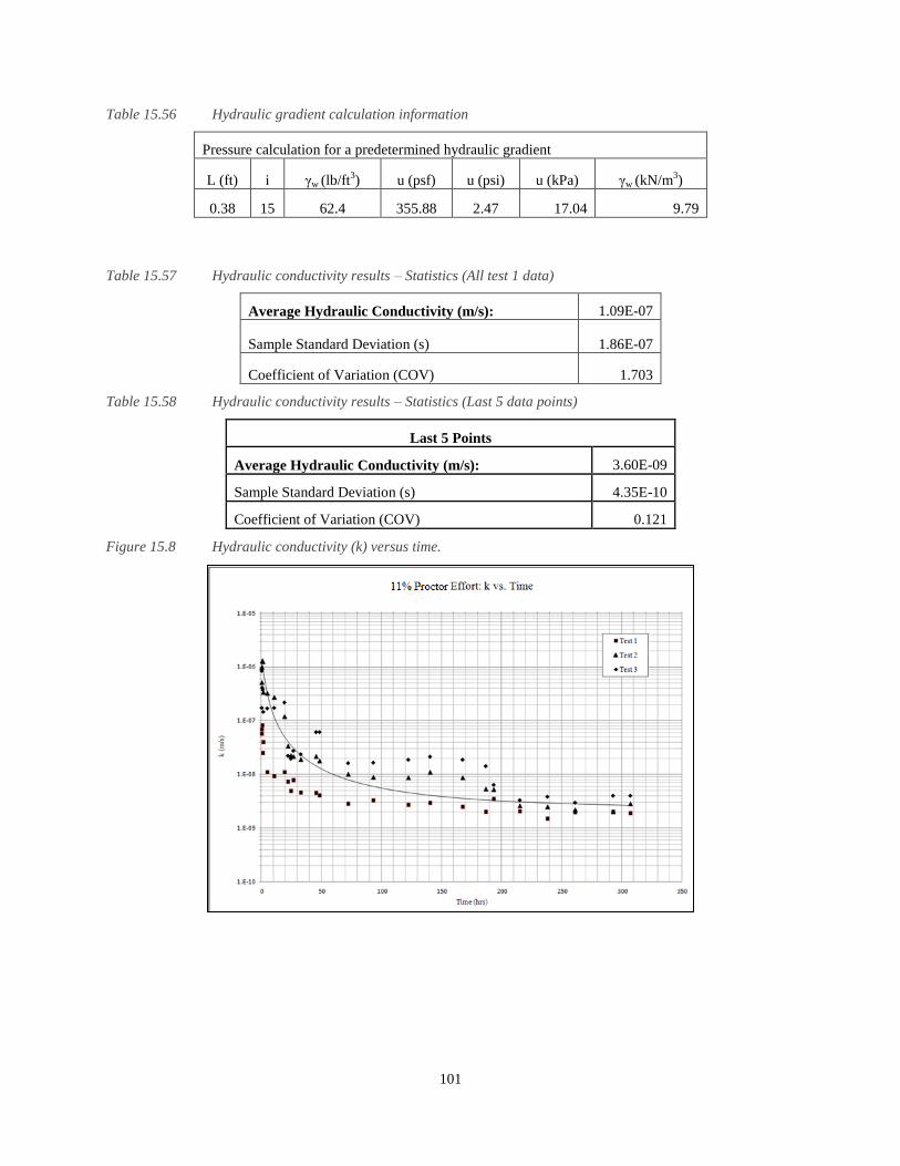
101
Table 15.56 Hydraulic gradient calculation information
Pressure calculation for a predetermined hydraulic gradient
L (ft) i γw (lb/ft3) u (psf) u (psi) u (kPa) γw (kN/m
3)
0.38 15 62.4 355.88 2.47 17.04 9.79
Table 15.57 Hydraulic conductivity results – Statistics (All test 1 data)
Average Hydraulic Conductivity (m/s): 1.09E-07
Sample Standard Deviation (s) 1.86E-07
Coefficient of Variation (COV) 1.703
Table 15.58 Hydraulic conductivity results – Statistics (Last 5 data points)
Last 5 Points
Average Hydraulic Conductivity (m/s): 3.60E-09
Sample Standard Deviation (s) 4.35E-10
Coefficient of Variation (COV) 0.121
Figure 15.8 Hydraulic conductivity (k) versus time.

102
Figure 15.9 Hydraulic conductivity (k) versus pore volumes (pV).
Table 15.59 Summary values for tests 1, 2, and 3.
i
γ11%Proctor
(kN/m3) γminimum (kN/m
3) e n k (m/s) s (for k) COV
Test 1 15 15.14 14.9 0.74 0.43 1.89E-09 2.37E-10 0.13
Test 2 15 15.52 14.9 0.70 0.41 2.43E-09 3.22E-10 0.13
Test 3 15 15.49 14.9 0.70 0.41 3.60E-09 4.35E-10 0.12
Average -- 15.38 -- 0.71 0.42 2.64E-09 3.31E-10 0.13
15.4 DISCUSSION
The hydraulic conductivity for each test performed for standard proctor, 34% proctor, and 11% proctor all remained
in the order of 10-9
m/s. The neither the 34% proctor permeated specimens, nor the standard proctor specimens had
hydraulic consolidation effects. Some hydraulic consolidation did occur for the 11% proctor specimens. The
consolidation that occurred was the cause of the low hydraulic conductivity of the 11% proctor specimens. The soil
structure could not retain its skeleton and void spaces collapsed under the hydraulic gradient of i=15. The standard
proctor and 34% proctor specimens had low porosities in a range of n=0.31 to n=0.38 which resulted in low
hydraulic conductivities. A summary table of the hydraulic conductivity results are shown in Table 15.60 below.
Table 15.60 Hydraulic conductivity summary
Test Number k (m/s)
Standard Proctor
Test 1 1.14E-09
Test 2 5.81E-09
Test 3 1.82E-09
34% Proctor
Test 1 2.02E-09
Test 2 1.69E-09
Test 3 3.31E-09
11% Proctor
Test 1 1.89E-09
Test 2 2.43E-09
Test 3 2.64E-09

103
16. POST-PERMEABILITY GRAIN SIZE DISTRIBUTION
Triplicate testing was performed for three phases of hydraulic conductivity testing. The first phase was a triplicate
testing of a standard proctor compacted specimen (592.5 kJ/m3) with a hydraulic gradient of i=100. For the first
phase, each specimen had a target density at the maximum dry density (18.75 kN/m3) of the determined proctor
curve. The second phase was a triplicate testing of a 34% Proctor compacted specimen (203.6 kJ/m3) with a
hydraulic gradient of i=15. For the second phase, each specimen had a target density at the maximum dry density
(18.1 kN/m3) of the determined proctor curve. The third phase was a triplicate testing of a 11% Proctor compacted
specimen (67.85 kJ/m3) with a hydraulic gradient of i=15. For the third phase, each specimen had a target density at
the minimum dry density (14.9 kN/m3) of the determined proctor curve. One hydraulic conductivity specimen was
chosen for each phase for grain size distribution testing. Three approximately equal layers were cut from the
specimen after the hydraulic conductivity had been determined. A sieve analysis was performed on each of these
layers. The objective of this testing was to determine the movement of the particles with an applied hydraulic
gradient that was comparable to the conditions that the material would experience in the field. These results have
implications on the stability or instability of earthen structures built from the unweathered sandstone under
inspection. The results of the testing are shown below.
16.1 POST-PERMEABILITY GRAIN SIZE DISTRIBUTION: STANDARD
PROCTOR (592.5KJ/M3)
Three approximately equal layers were cut from the standard proctor Test 1 hydraulic conductivity specimen in
Chapter 10, section 10.1 for the standard proctor post-permeability grain size distribution testing. The layers were
tested separately to determine whether or not their gradations varied. The sought after variation is a result of particle
movement during permeation. Only the sand portion (passing #4 sieve to #200 sieve) was permeated and tested.
The results of the sieve analysis yielded a coefficient of variation of 0.036 for the uniformity coefficient and a
coefficient of variation of 0.044 for the coefficient of gradation. This low coefficient of variation implies that the
samples had very little variation in their gradations. Additional information about the properties of this specimen
can be found in Appendix I and section 10.1. The data for the sieve analysis is shown in the tables and figure below.
Table 16.1 Critical index values for the hydraulic conductivity grain size distribution testing.
Critical Indices Layer 1 Layer 2 Layer 3
D90 3.90 4.00 4.00
D60 2.00 2.40 2.30
D50 1.60 1.80 1.75
D30 0.74 0.83 0.81
D25 0.60 0.65 0.65
D10 0.14 0.16 0.15
Uniformity Coefficient, Cu 14.29 15.00 15.33
Coefficient of Gradation, Cc 1.96 1.79 1.90
Table 16.2 Uniformity coefficient statistics
Uniformity Coefficient, Cu
Average Uniformity Coefficient 14.873
Sample Standard Deviation (s) 0.535
Coefficient of Variation (COV) 0.036
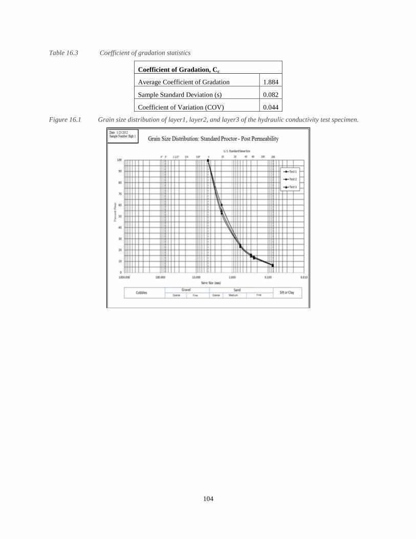
104
Table 16.3 Coefficient of gradation statistics
Coefficient of Gradation, Cc
Average Coefficient of Gradation 1.884
Sample Standard Deviation (s) 0.082
Coefficient of Variation (COV) 0.044
Figure 16.1 Grain size distribution of layer1, layer2, and layer3 of the hydraulic conductivity test specimen.

105
16.2 POST-PERMEABILITY GRAIN SIZE DISTRIBUTION: 34%
PROCTOR (203.6 KJ/M3)
Three approximately equal layers were cut from the 34% proctor Test 1 hydraulic conductivity specimen in Chapter
10, section 10.2 for the standard proctor post-permeability grain size distribution testing. The layers were tested
separately to determine whether or not their gradations varied. The sought after variation is a result of particle
movement during permeation. Only the sand portion (passing #4 sieve to #200 sieve) was permeated and tested.
The results of the sieve analysis yielded a coefficient of variation of 0.163 for the uniformity coefficient and a
coefficient of variation of 0.050 for the coefficient of gradation. This low coefficient of variation implies that the
samples had very little variation in their gradations. Additional information about the properties of this specimen
can be found in Appendix I and section 10.2. The data for the sieve analysis is shown in the tables and figure below.
Table 16.4 Critical index values for the hydraulic conductivity grain size distribution testing.
Critical Indices Layer 1 Layer 2 Layer 3
D90 3.900 3.900 4.000
D60 2.100 2.200 2.400
D50 1.600 1.700 1.800
D30 0.660 0.700 0. 880
D25 0.500 0.550 0.700
D15 0.230 0.260 0.350
D10 0.110 0.130 0.175
Uniformity Coefficient, Cu 19.09 16.92 13.71
Coefficient of Gradation, Cc 1.89 1.71 1.84
Table 16.5 Uniformity coefficient statistics
Uniformity Coefficient, Cu
Average Uniformity Coefficient 16.576
Sample Standard Deviation (s) 2.705
Coefficient of Variation (COV) 0.163
Table 16.6 Coefficient of gradation statistics
Coefficient of Gradation, Cc
Average Coefficient of Gradation 1.814
Sample Standard Deviation (s) 0.090
Coefficient of Variation (COV) 0.050

106
Figure 16.2 Grain size distribution of layer1, layer2, and layer3 of the hydraulic conductivity test specimen.

107
16.3 POST-PERMEABILITY GRAIN SIZE DISTRIBUTION: 11%
PROCTOR (67.85 KJ/M3)
For 11% proctor hydraulic conductivity, a sieve analysis was performed for three permeated specimens with three
layers each for additional precision in the testing. Test 1, Test 2, and Test 3 correspond to Tests 1, 2, and 3 in
sections 10.3.1, 10.3.2, and 10.3.3, respectively. Compaction information, porosity (n), void ratio (e), and other
properties of each specimen are given in each respective section as well as Appendix I. Three approximately equal
layers were cut from the hydraulic conductivity specimen in Chapter 10 for the standard proctor post-permeability
grain size distribution testing. The layers were tested separately to determine whether or not their gradations varied.
The sought after variation is a result of particle movement during permeation. Only the sand portion (passing #4
sieve to #200 sieve) was permeated and tested.
16.3.1 POST-PERMEABILITY GRAIN SIZE DISTRIBUTION: 11%
PROCTOR - TEST 1
The results of this sieve analysis yielded a coefficient of variation of 0.096 for the uniformity coefficient and a
coefficient of variation of 0.067 for the coefficient of gradation. This low coefficient of variation implies that the
samples had very little variation in their gradations. The data for the sieve analysis is shown in the tables and figure
below.
Table 16.7 Critical index values for the hydraulic conductivity grain size distribution testing.
Results
Critical Indices Layer 1 Layer 2 Layer 3
D90 3.750 3.900 3.800
D60 1.750 2.000 1.900
D50 1.300 1.500 1.400
D30 0.590 0.630 0.650
D25 0.430 0.480 0.500
D15 0.180 0.210 0.240
D10 0.095 0.105 0.120
Uniformity Coefficient, Cu 18.42 19.05 15.83
Coefficient of Gradation, Cc 2.09 1.89 1.85
Table 16.8 Uniformity coefficient statistics
Uniformity Coefficient, Cu
Average Uniformity Coefficient 17.767
Sample Standard Deviation (s) 1.704
Coefficient of Variation (COV) 0.096
Table 16.9 Coefficient of gradation statistics
Coefficient of Gradation, Cc
Average Coefficient of Gradation 1.946
Sample Standard Deviation (s) 0.130
Coefficient of Variation (COV) 0.067

108
Figure 16.3 Grain size distribution of layer1, layer2, and layer3 of the hydraulic conductivity test specimen.

109
16.3.2 POST-PERMEABILITY GRAIN SIZE DISTRIBUTION: 11%
PROCTOR - TEST 2
The results of this sieve analysis yielded a coefficient of variation of 0.065 for the uniformity coefficient and a
coefficient of variation of 0.058 for the coefficient of gradation. This low coefficient of variation implies that the
samples had very little variation in their gradations. The data for the sieve analysis is shown in the tables and figure
below.
Table 16.10 Critical index values for the hydraulic conductivity grain size distribution testing.
Critical Indices Layer 1 Layer 2 Layer 3
D90 3.800 3.800 3.900
D60 1.800 1.700 1.900
D50 1.400 1.400 1.450
D30 0.600 0.590 0.600
D25 0.470 0.450 0.480
D15 0.190 0.190 0.200
D10 0.094 0.100 0.100
Uniformity Coefficient, Cu 19.15 17.00 19.00
Coefficient of Gradation, Cc 2.13 2.05 1.89
Table 16.11 Uniformity coefficient statistics
Uniformity Coefficient, Cu
Average Uniformity Coefficient 18.383
Sample Standard Deviation (s) 1.200
Coefficient of Variation (COV) 0.065
Table 16.12 Coefficient of gradation statistics
Coefficient of Gradation, Cc
Average Coefficient of Gradation 2.023
Sample Standard Deviation (s) 0.118
Coefficient of Variation (COV) 0.058

110
Figure 16.4 Grain size distribution of layer1, layer2, and layer3 of the hydraulic conductivity test specimen.

111
16.3.3 POST-PERMEABILITY GRAIN SIZE DISTRIBUTION: 11%
PROCTOR - TEST 3
The results of this sieve analysis yielded a coefficient of variation of 0.121 for the uniformity coefficient and a
coefficient of variation of 0.017 for the coefficient of gradation. This low coefficient of variation implies that the
samples had very little variation in their gradations. The data for the sieve analysis is shown in the tables and figure
below.
Table 16.13 Critical index values for the hydraulic conductivity grain size distribution testing.
Critical Indices Layer 1 Layer 2 Layer 3
D90 3.900 4.000 4.000
D60 1.900 2.200 2.400
D50 1.450 1.700 1.900
D30 0.650 0.680 0.800
D25 0.520 0.520 0.620
D15 0.240 0.220 0.280
D10 0.120 0.110 0.140
Uniformity Coefficient, Cu 15.83 20.00 17.14
Coefficient of Gradation, Cc 1.85 1.91 1.90
Table 16.14 Uniformity coefficient statistics
Uniformity Coefficient, Cu
Average Uniformity Coefficient 17.659
Sample Standard Deviation (s) 2.131
Coefficient of Variation (COV) 0.121
Table 16.15 Coefficient of gradation statistics
Coefficient of Gradation, Cc
Average Coefficient of Gradation 1.89
Sample Standard Deviation (s) 0.032
Coefficient of Variation (COV) 0.017

112
Figure 16.5 Grain size distribution of layer1, layer2, and layer3 of the hydraulic conductivity test specimen.

113
17. GRADING ENVELOPES AND PARTICLE TRANSPORT
17.1 INTRODUCTION
The term “grading envelope” refers to the range, or variation, of particle size with respect to the percent finer of
the material being observed. Grading envelopes can be a result of a phenomenon called suffusion. Suffosion is
defined as the transportation of soil particles over significant distances through constrictions within a soil
matrix. If the constrictions are larger than the particle, then the particle has the potential to be transported, and
sometimes exit the soil body it is encased within. It is understood that particle transport can clog a filter if a soil
is regarded as unstable. Unstable soils are those which have significant particle movement, where the soil
acting as a filter will become more porous due to a loss of fine particles. An increase in porosity and a potential
increase in pore pressure at the toe of a slope due to an accumulation of fine particles, or clogging of the filter,
can compromise the stability of a slope structure. This section compiles data accrued in the laboratory testing
performed for this project. The purpose of the data is to illustrate the movement of soil particles under several
imposed conditions, or lack thereof, to determine whether or not suffusion has the potential to be a significant
concern in the stability modeling of the unweathered sandstone overburden under inspection. The data on the
nine graphs below show the results of grain size distribution testing performed on layering of compacted
specimens at three predetermined compaction energies. The energy levels are referred to as standard proctor at
a compaction energy of 592.5 kJ/m3, a 65.64% reduced from standard proctor effort or 34.36% of standard
proctor or 203.6 kJ/m3), and an even further reduced energy at 88.55% reduced equal to 67.85 kJ/m
3 or 11.45%
of standard proctor energy. Three tests are shown per graph. The three tests are as received GSD, pre-
permeability GSD, and post-permeability GSD. Layer 1, 2, and 3 are approximately one-third the length of the
compacted specimen, and are top one-third, middle one-third, and bottom one-third, respectively.

114
17.2 STANDARD PROCTOR GSD RESULTS
The figures below show graphs of superimposed grain size distributions. The grain size distributions illustrate
the process of as received to a compaction to condition to a permeated condition. The item “Δ” in the figures
means simply “the change in” for each maximum aggregation compared to the as received grain size
distribution for the critical index shown. This value is expressed as a percent difference. Smaller values of “Δ”
are lesser aggregation conditions, and larger values refer to larger changes in aggregation. The two graphs
shown below illustrate some interesting phenomena. Let us consider the first illustration showing the grain size
distribution of three layers of a compacted sample prepared as a standard proctor specimen alongside the
original grain size distribution of the material. The material had 9.04% water content added to it. The material
aggregated some, and was not particularly isotropic. The second illustration had 8.43% water content after
distilled water was added to the sample, and it was compacted. The post-permeability grain size distribution
became more aggregated after being permeated by 18.46 pore volumes. The material aggregation seems to be a
function of the compaction energy and the water content. The compaction energy applied in the first illustration
likely broke up the aggregation of the material, where the aggregation could reconvene in the hydraulic
conductivity cell in the second illustration.
Figure 17.1 Standard Proctor grain size distribution compilation

115
17.3 34% PROCTOR ENERGY GSD RESULTS
The two illustrations below depict the variations in gradation for two samples of a well graded sand with silt
material compared to the original gradation of the material. The first graph is at a pre-permeability or pre-
permeability state, and the second is at a post-permeability state. Both samples had a target dry density at optimum
of a set 34% Proctor compaction effort of 203.6 kJ/m3. The pre-permeability sample had a water content of 13.16%.
The post-permeability sample had a pre-permeated water content of 14%. The permeated sample had 2.22 pore
volumes run through it. The behavior of the material under these conditions seems to indicate that the compaction
and added water increased the aggregation of the material. The permeation increased the aggregation more than the
compaction alone. Similar behavior occurred in the standard proctor samples.
Figure 17.2 34% Proctor compaction energy grain size distribution compilation
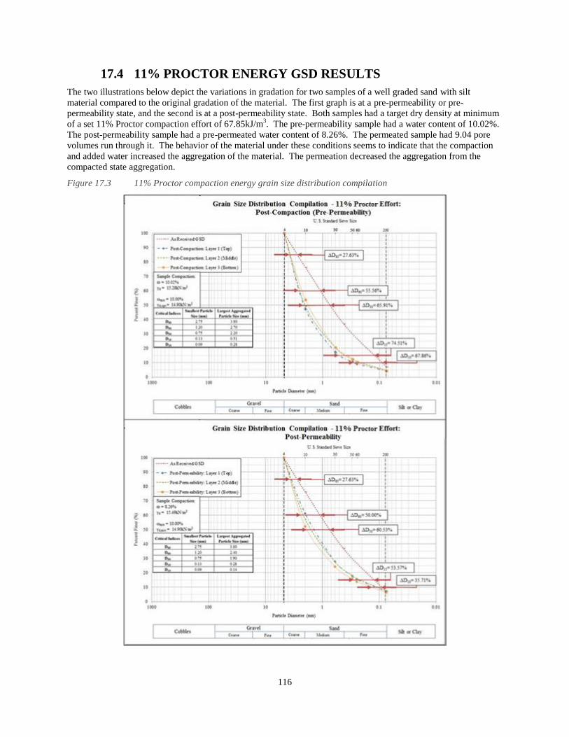
116
17.4 11% PROCTOR ENERGY GSD RESULTS
The two illustrations below depict the variations in gradation for two samples of a well graded sand with silt
material compared to the original gradation of the material. The first graph is at a pre-permeability or pre-
permeability state, and the second is at a post-permeability state. Both samples had a target dry density at minimum
of a set 11% Proctor compaction effort of 67.85kJ/m3. The pre-permeability sample had a water content of 10.02%.
The post-permeability sample had a pre-permeated water content of 8.26%. The permeated sample had 9.04 pore
volumes run through it. The behavior of the material under these conditions seems to indicate that the compaction
and added water increased the aggregation of the material. The permeation decreased the aggregation from the
compacted state aggregation.
Figure 17.3 11% Proctor compaction energy grain size distribution compilation

117
17.5 DISCUSSION
Comparatively, taking into consideration all three compaction energies and the results shown above of the test
scenarios performed it was found that particle movement varied significantly. The variation in gradation was a
function of the moisture content added and the energy applied for preparation. The post-permeability results should
be interpreted carefully as each specimen of different density varied in pore volume flux. The standard proctor
specimens aggregated the most between D50 and D15 due to compaction, then aggregated more at a post-permeability
condition. The 34% Proctor compaction specimens showed similar results as standard proctor, aggregating more at
a post-permeability condition. The 11% Proctor compaction specimen results were opposite 34% Proctor
compaction results and standard proctor compaction results. The 11% Proctor compaction specimen aggregated
most at a pre-permeability condition, then became less aggregated at a post-permeability condition. The results
indicate that the material reaches an aggregated equilibrium with very similar gradation after some pore volumes of
water permeate through it. The results also imply that introducing a range of compaction energy can alter soil
properties and have performance implications on earthen structures. Layered construction known as “lift
construction” could assist in better quality control of the compaction energy applies to earthen structures to more
precisely manage the aggregation phenomena. The amount of compaction energy for the 34% Proctor compaction
and standard proctor samples seems to have broken up the aggregated particles, then when they were permeated,
became more aggregated. After the permeation occurred, all three compaction energies approached a similar
gradation, but diverged somewhat as the particle size decreased. The specimens began diverging in similarity
around 40% finer. At D10 at a post-permeability condition, the 11% Proctor compaction energy compacted and
permeated sample had the smallest particles, standard proctor had the next highest, and 34% Proctor energy
specimens had the largest particle size. Overall the 11% proctor pre-permeability condition had the most aggregated
particles, likely due to little compaction energy applied to break apart aggregated particles. At D10 at a pre-
permeability condition, the standard proctor sample had the smallest particles, then 34% proctor, and 11% Proctor
energy samples had the largest aggregated particles. The item “Δ” in the figures means simply “the change in” for
each maximum aggregation compared to the as received grain size distribution for the critical index shown. This
value is expressed as a percent difference. Smaller values of “Δ” are lesser aggregation conditions, and larger values
refer to larger changes in aggregation. The table below shows a summary of the delta values for Figure 17.1, Figure
17.2, and Figure 17.3.
Table 17.1 Change in critical index summary table
Change in
Critical Indices
[%]
ΔD85
(%)
ΔD60
(%)
ΔD50
(%)
ΔD15
(%)
ΔD10
(%)
Standard Proctor
Pre-Permeability 12.73 41.67 48.89 53.57 40.00
Standard Proctor
Post-Permeability 27.63 50.00 58.33 58.06 43.75
34% Proctor
Pre-Permeability 19.12 33.33 46.43 53.57 47.06
34% Proctor
Post-Permeability 25.68 50.00 58.33 62.86 48.57
11% Proctor
Pre-Permeability 27.63 55.56 65.91 74.51 67.86
11% Proctor
Post-Permeability 27.63 50.00 60.53 53.57 35.71

118
18. SEEP/W ANALYSIS
The hydrologic conditions for the valley fill site were determined as inputs for seepage modeling. This consisted of
identifying actual precipitation totals and runoff characteristics of the site to develop infiltration functions for
individual storm events. This data was used in later development of boundary conditions for the numerical model.
A comprehensive seepage and slope stability analysis was then developed using the SEEP/W, SIGMA/W, and
SLOPE/W modules of GeoStudio2007. These analyses were performed for the AOC and geomorphic fill designs.
After completion of the numerical modeling, data was reduced for the results of each of the two fills. Results were
then compared in tabular and graphical form to find benefits and contrasts to the AOC and geomorphic designs.
18.1 UNSATURATED SOIL PROPERTY FUNCTIONS
When modeling with saturated and unsaturated soil cycles, it is sometimes necessary to approximate functions for
soil properties to input into the numerical model. These include the soil-water characteristic curve (water content vs.
matric suction) and hydraulic conductivity functions (hydraulic conductivity vs. matric suction) of the soil. A study
by Fredlund et al. (1997) discussed these issues. Fredlund stated that the soil-water characteristic curve has become
very useful in the estimation of unsaturated soil property functions. Numerical modeling requires the use of
nonlinear soil property functions when unsaturated soils are analyzed. This method seems to be gaining acceptance
in the analysis of unsaturated soil systems in engineering practice. Fredlund stated that the behavior of unsaturated
soils is a function of pore size geometry and distribution. The soil-water characteristic curve has become the main
method for understanding this relationship and is used to compute approximate soil property functions in
unsaturated soils. Unsaturated soil property functions plot unsaturated soil properties versus soil suction. Examples
of soil property functions are coefficient of permeability, coefficient of water volume change, and shear strength.
These properties can be easily tested in the laboratory, but a way to economically complete the tests has not yet been
determined. Unsaturated soil property tests can be costly. For this reason, the use of the soil-water characteristic
curve to predict unsaturated soil property functions has been investigated. Some inaccuracies may be associated
with this method, but the cost of these inaccuracies are outweighed by the benefits of the savings in cost.
Fredlund et al. (1997) stated that the use of “knowledge-based system” was the most effective method of
determining unsaturated soil property functions. A knowledge-based system uses a database of soils whose soil-
water characteristic curves have already been classified. Three procedures can use the database to obtain unsaturated
soil property functions. First, a measured soil-water characteristic curve could be directly matched to a soil-water
characteristic curve already in the database. The second method consisted of using measured soil classification
properties to match with one of more soils in the database and therefore match to a soil-water characteristic curve.
The third procedure involved comparing the soil’s grain size distribution curve the grain size curves of soils in the
database. Once the corresponding soil-water characteristic curve was found, the appropriate unsaturated soil
properties could be computed. These methods were found to have several advantages. The estimation of the
unsaturated soil properties was quickly available, cost efficient, and easily completed by inexperienced
professionals. Fredlund (1997) stated that the program SoilVision used a database of over 600 soils to estimate
unsaturated soil property functions using a knowledge-based approach.
Fredlund (1997) used an environmental application example to demonstrate the use of this knowledge-based system.
Water seepage through mine tailings of a mine site in Papua, New Guinea was analyzed. A steady state and
transient analysis were conducted. The steady state analysis used rainfall totals to determine the location of the
water table. The transient analysis simulated a drought that desaturated the tailings. The transient analysis required
the estimation of a soil-water characteristic curve and hydraulic conductivity curve. The mine tailings were found to
have a void ratio of 0.80, a saturation of 98%, and a specific gravity of 2.66. A grain size-distribution for the
tailings was also developed. These soil properties were input into SoilVision and used to classify the soil. The
tailings were classified as a sand. SoilVision then used the volume-mass properties and grain-size distribution to
predict the soil-water characteristic curve using the van-Genuchten equation and a saturated volumetric water
content of 44%. Next, the hydraulic conductivity for the soil was developed. SoilVision used the soil’s saturated
hydraulic conductivity (1.1 x 10^-5 m/s) and the soil-water characteristic curve to estimate the full hydraulic
conductivity curve. These soil property functions were then input as the material properties in a transient
groundwater seepage analysis using the SEEP/W module of GeoStudio™.
The following conclusions were made from this study: the soil-water characteristic curve is valuable in estimating
unsaturated soil property functions; non linear soil property functions are necessary in numerical modeling,

119
particularly transient groundwater seepage; a “knowledge-based approach” for determining unsaturated soil property
functions is advantageous to determining the properties using laboratory testing; a “knowledge-based approach” can
be used to adequately develop a soil-water characteristic curve and hydraulic conductivity curve for the numerical
modeling of seepage through mine waste rock.
18.2 SITE HYDROLOGY
To fully classify the site before modeling, the hydrology of the site had to be fully defined. Defining the hydrology
of the site was necessary to determine the inputs for later modeling. This process consisted of using precipitation
data and runoff characteristics to determine what amount and at what rate water infiltrates into the fill.
Precipitation
Hydrologic information was obtained from the National Oceanic and Atmospheric Administration (2012). Archived
daily precipitation data was found using an interactive map of the GHCN (Gloabal Historical Climatology Network)
Daily precipitation data for the Logan, WV (46-5353) station. This is the closest station to the surface mine of
interest. Daily precipitation totals were downloaded from January 1, 2001 – December 31, 2010. The data was
compared to a previous study using 2010 precipitation data. Meek and O’dell (2012) used a total precipitation of
45.87 inches for 2010, which compared well to the value of 48.95 inches from NOAA. For each of these 10 years,
precipitation over time was graphed. Figure 18.1 is the rainfall graph for the year 2001, which was used later for
infiltration functions:
Figure 18.1 2001 rainfall totals for Logan, WV
Infiltration from Storm Events
Rainfall intensities for specific storm types (100-yr, 24-hr; 500-yr, 24-hr) were taken from the IDF (intensity-
duration-frequency) table from NOAA’s Precipitation Frequency Data Server (2012). This data was also taken from
the Logan, WV station. For the transient condition, infiltration was determined as a function of time. This first step
in developing this function was to find the infiltration function for different storm events. Frequencies of 2, 10, 25,
50, 100, and 500 years were analyzed for both 1 hr and 24 hr durations. These storms were modeled using the
Horton infiltration capacity equation:
Where,
0
10
20
30
40
50
60
70
1-Jan 1-Feb 1-Mar 1-Apr 1-May 1-Jun 1-Jul 1-Aug 1-Sep 1-Oct 1-Nov 1-Dec
Rai
nfa
ll (
mm
)
Date
Rainfall Totals: 2001

120
⁄ ⁄
⁄
Huber and Dickinson (1998) stated that the value of the k constant should be taken as 4.14/hr in the absence on field
data. For this reason, 4.14/hr was used as the k value for modeling. The final infiltration capacity was taken as the
saturated hydraulic conductivity. Hydraulic conductivity was chosen from a range values found from previous work
done with waste rock tailings. These ranged from an unsaturated hydraulic conductivity of 1x10^-5 m/s taken from
a study by Abdelghani (2009) to a saturated hydraulic conductivity of 1x10^-7 m/s taken from Aubertin et al.
(1996). These previously published values were chosen instead of the values determined from laboratory testing
because they represented actual data used in practice. Laboratory testing calculates hydraulic conductivity based on
optimum water content and compaction values, which are difficult to obtain in the field. Previously published
values for hydraulic conductivity of waste rock tailings provided a more practical value to be used in numerical
modeling. For each storm, the lowest value between the rainfall intensity and the unsaturated hydraulic conductivity
of 1x10^-5 m/s was used as the initial infiltration capacity. This is because the fastest that water can infiltrate is at
the magnitude of the unsaturated hydraulic conductivity. Figure 18.2 below plots infiltration versus time for the 1 hr
storms:
Figure 18.2 Horton infiltration function – 1 hour storms
For the 1 hr storms, the initial infiltration capacity was equal to the unsaturated hydraulic conductivity (1 x 10^-5
m/s) for all storms except the 2 year storm. This is because every storm other than the 2 year storm had a rainfall
intensity of greater than the unsaturated hydraulic conductivity. As the soil became saturated, the rate at which the
water was able to infiltrate decreased until all storms approached the same final infiltration capacity at the end of 1
hour. This final infiltration capacity was equal to the saturated hydraulic conductivity (1 x 10^-7 m/s).
Figure 18.3 below shows the plot of infiltration versus time for the 24-hr storms:
0
0.000002
0.000004
0.000006
0.000008
0.00001
0.000012
0 10 20 30 40 50 60
Infi
ltra
tio
n (
m/s
)
Time (min)
Horton Infiltration (1-hr Storms)
2 yr
10 yr
25 yr
50 yr
100 yr
500 yr

121
Figure 18.3 Horton infiltration function – 24 hour storms
For the 24-hr storms, all frequency storms had an initial infiltration capacity equal to the rainfall intensity. This was
because each storm had a rainfall intensity less than the unsaturated hydraulic conductivity. Each storm reached the
final infiltration capacity (saturated hydraulic conductivity) of the soil within 1 hr.
18.3 SEEPAGE MODELING APPROACH
The numerical model used to analyze the fills was the finite element model of GeoStudio 2007. Modeling in
GeoStudio requires three general steps. First, the geometry of the model must be identified and discretized into
elements. After that has been done, material properties must be defined and then boundary conditions applied.
Modeling was done for both an AOC fill and a geomorphic fill, which are described in detail in the section. The
SEEP/W module was used to analyze the fill with regards to seepage.
Geometry
For any modeling to be completed, the geometry of both the AOC and geomorphic fills first had to be defined. The
geometry of each fill was taken from plan view contours. A profile slice was taken alone the centerline of the slope,
as to produce the longest profile slice within the fill and to include the drain within the fill. In SEEP/W, the profile
uses a default thickness of 1 meter to calculate volumes. Defining the geometry consisted of three regions.
1. A foundation rock region (original ground)
2. A fill material region above the foundation rock
3. A blocky core drain between the foundation rock and fill material
An approximate global mesh size of 10 m was used. Figure 18.4 and Figure 18.5 below are the profiles from
SEEP/W for each fill with axes to show size. The three distinct regions can be seen. Following the figures are
explanations of how each fill’s geometry was defined.
0
0.0000005
0.000001
0.0000015
0.000002
0 1 2 3 4 5
Infi
ltra
tio
n (
m/s
)
Time (hr)
Horton Infiltration (24-hr Storms)
2 yr
10 yr
25 yr
50 yr
100 yr
500 yr

122
Figure 18.4 AOC fill geometry
Figure 18.5 Geomorphic fill geometry

123
18.4 GROUNDWATER SEEPAGE MODELING
SEEP/W was the module used to model groundwater seepage in a 2-dimensional state. SEEP/W uses material
properties and boundary conditions to generate contours and x-y plots of parameters such as head, pressure,
gradient, velocity, and hydraulic conductivity. A transient condition can be applied to model a changing water table
over time. Seepage for the valley fill was analyzed in a transient condition over the span of 10 years using finite
element modeling. 10 time steps were modeled to produce model results for each of the 10 years. A maximum of
50 iterations was chosen with a maximum of 5 reviews per time step. Initial pore-water pressure conditions were set
to be taken from a manually input initial water table. With the geometry of each fill already defined, the next step
was the next step was defining the material properites. Finally, by developing the site hydrology, boundary
conditions were applied.
Materials
The valley fill model consisted of three materials:
1. Fill
2. Foundation Rock
3. Blocky Core Drain
For both fills, each material was given the same properties because the same materials were used in both designs.
These materials for each fill can be seen Figure 18.6 and Figure 18.7 below.
Figure 18.6 AOC fill materials
Figure 18.7 Geomorphic fill materials
The first material, named “Fill”, was the top layer of the valley fill comprised of waste rock tailings from mining. It
was modeled under a saturated/unsaturated condition. This allowed the material to begin in an unsaturated state and
become saturated over time. Modeling in the saturated/unsaturated condition required a function for hydraulic
conductivity and water content. Hydraulic conductivity (m/s) was plotted versus pore water pressure (kPa) by
inputting a saturated hydraulic conductivity and using the van-Genuchten estimation method within SEEP/W. A
maximum suction was set at 0.01 kPa and a minimum set at 1000 kPa with 20 data points to produce a function.
Hydraulic conductivity was chosen from a range values found from previous work done with waste rock tailings.
These ranged from an unsaturated hydraulic conductivity of 1x10^-5 m/s (Abdelghani 2009) to a saturated hydraulic
conductivity of 1x10^-7 m/s (Aubertin et al 1996). The function is shown in Figure 18.8 below.

124
Figure 18.8 Fill conductivity function – AOC fill
This function was also compared to the function produced by Fredlund et al (1998) and found to be quite similar.
The water content function (soil-water characteristic curve) was produced in a similar method. A saturated
volumetric water content was input and the same parameters as the conductivity function were used to create a
function. Sand was chosen as the material type for this function to correspond with soil classification of “well
graded sand” that was determined in laboratory testin. Saturated volumetric water content was taken to be 44%, the
value used by Fredlund et al (1998). This function is shown in Figure 18.9 below.
Figure 18.9 Fill water content function – AOC fill
1.00E-36
1.00E-33
1.00E-30
1.00E-27
1.00E-24
1.00E-21
1.00E-18
1.00E-15
1.00E-12
1.00E-09
1.00E-06
1.00E-03
1.00E+00
0.01 0.1 1 10 100 1000
Hyd
rauli
c C
ond
uct
ivit
y (
m/s
)
Matric Suction (kPa)
Fill Conductivity
0
0.05
0.1
0.15
0.2
0.25
0.3
0.35
0.4
0.45
0.5
0.01 0.1 1 10 100 1000
Wat
er C
onte
nt
(m^3
/m^3
)
Matric Suction (kPa)
Fill Water Content

125
The bottom layer of the valley fill, the “Foundation Rock” layer, was modeled in a saturated only condition with a
very low hydraulic conductivity (2x10^12 m/s) to simulate an impermeable rock layer. Between the “Fill” layer and
“Foundation Rock” layer, a 10-ft “Blocky Core Drain” material was placed. This layer was modeled under a
saturated only condition with a constant hydraulic conductivity value of 0.1 m/s. This hydraulic conductivity was
taken from the Das (2010) average value for gravel. Table 18.1 below summarizes the inputs used to define the
material properties of each fill.
Table 18.1 SEEP/W material inputs
Material Fill Foundation
Rock
Blocky Core
Drain
Condition saturated/unsaturated saturated only saturated only
Hydraulic
Conductivity
Modeling
function constant constant
Unsaturated
Hydraulic
Conductivity (m/s)
1.00E-05 NA NA
Saturated
Hydraulic
Conductivity
1.00E-07 2.00E-12 0.1
18.5 BOUNDARY CONDITIONS
Once materials and site hydrology were defined, boundary conditions were determined to fully define the model. To
do this, an infiltration function was developed from the NOAA precipitation data. It is important to note that the
SEEP/W analysis did not take into account any stream infiltration, only infiltration from precipitation. For modeling
a valley fill, two different infiltration functions had to be developed:
1. A function for water infiltrating on a flat surface (the top of the fill)
2. A function for water infiltrating on a sloped surface (the face of the fill)
A study by Sharma et al (2009) states that the infiltration ranges from 75-95% of the accumulated rainfall. For the
top of the slope, each daily rainfall value was multiplied by an average value of 85% to obtain the infiltration depth.
Studies by Ziemkiewicz (2011) and Meek and O’dell (2012) stated that the percentage of precipitation on the face of
a fill that infiltrates the surface was 52% and 58%, respectively. Using these values, the daily precipitation totals
were multiplied by 0.55 (average of the two values) to determine the amount of rainfall that infiltrated into the
sloped portion of the fill. To determine how long precipitation from a given storm infiltrated, the precipitation depth
was compared to the unsaturated hydraulic conductivity. With an unsaturated hydraulic conductivity of 36 mm/hr
(determined by performing unit conversion on 1 x10^-5 m/s), any precipitation depth of less than 36 mm would take
less than 1 hour to infiltrate fully. To maintain a minimum time step of 1 hour within the model, any precipitation
depth of 36 mm or less was given a duration of 1 hour. Any precipitation depth of greater than 36 mm was divided
by 36 mm/hr to determine the duration. Once all durations were calculated each infiltration depth was divided by its
duration to determine the infiltration rate in m/s. As seen in the Horton infiltration functions for all design storms,
any storm that had an infiltration function of greater than the saturated hydraulic conductivity (1 x 10^-7 m/s) had an
infiltration function that decreased to the magnitude of the saturated hydraulic conductivity after one hour. Each
duration, for this reason, was given the initial calculated infiltration rate followed by an infiltration rate of 1 x 10^-7
m/s after one hour. This infiltration rate then continued for the remainder of the infiltration duration.

126
A spreadsheet was then developed for one year’s worth of precipitation data depicting infiltration rate over time for
both the 85% infiltration and 55% infiltration. On day one of the 55% infiltration function, for example, water
infiltrated at 1.22 x 10^-7 m/s then decreased to 1x10^-7 m/s after one hour, followed by an infiltration of 0 m/s for
the remaining 23 hours of the day. At the beginning of day two, infiltration began again at 7.64 x 10^-8 m/s. The
two infiltration functions for one year can be seen in Figure 18.10 and Figure 18.11 below:
Figure 18.10 55% infiltration function for valley fill
Figure 18.11 85% infiltration function for valley fill
0.00E+00
2.00E-07
4.00E-07
6.00E-07
8.00E-07
1.00E-06
1.20E-06
0 50 100 150 200 250 300 350
Infi
ltra
tio
n (
m/s
)
Time (days)
Infiltration Function - 55% Infiltration
0.00E+00
2.00E-07
4.00E-07
6.00E-07
8.00E-07
1.00E-06
1.20E-06
0 50 100 150 200 250 300 350
Infi
ltra
tio
n (
m/s
)
Time (days)
Infiltration Function - 85% Infiltration

127
These one year functions were repeated ten times in order to be used in a model that spanned ten years. These ten
year infiltration functions were then keyed into SEEP/W as a step data point function for infiltration (unit flux vs.
time) to produce the infiltration boundary conditions.
The boundary conditions and their applied locations for each fill are shown in Figure 18.12 and Figure 18.13 below.
The locations of their applications are described following the figures.
Figure 18.12 AOC fill boundary conditions
Figure 18.13 Geomorphic fill boundary conditions
For the AOC fill, the 85% infiltration function boundary condition was applied to the top of the fill, and the 55%
infiltration designation was applied to the downstream sloped face of the fill. The 55% infiltration function
boundary condition placed on the fill’s downstream face was also analyzed as a potential seepage face. A constant
head function was applied at the toe of the fill to model the discharge pond. The head value was input as the
elevation of the discharge pond. Groundwater seepage modeling with SEEP/W also required inputting an initial
water table. The water table was placed at a constant level through the foundation rock at the elevation of the
discharge pond. A closer view of the boundary conditions at the toe of the fill is shown in Figure 18.14 below.
Figure 18.14 AOC boundary conditions at toe

128
The same boundary conditions were used to define the geomorphic model as were used in the AOC model. For this
case, however, the entire fill surface used the 55% infiltration boundary condition because it is sloped for its entire
length. The sloped fill surface was also analyzed as a potential seepage face. Due to the altered surface profile, the
initial water table and discharge pond were modeled at a height of 353.57 m, slightly lower than in the AOC fill. A
closer view of the boundary conditions at the toe of the fill is shown in Figure 18.15 below.
Figure 18.15 Geomorphic fill boundary conditions at toe

129
18.6 Groundwater Seepage Results
The following section discusses the results of groundwater seepage modeling using SEEP/W. First the individual
criteria by which the fills were analyzed are defined. Next, how to interpret the visual results of modeling profiles is
explained. Then, visual and tabular results are organized and presented. Finally, the results for the AOC fill and
geomorphic fill are compared in order to obtain any significant findings.
Criteria for Analysis
In order to analyze the AOC and geomorphic fill on a year-to-year basis for each of the 10 years, parameters had to
be chosen by which to analyze and compare. These parameters included:
Minimum and maximum pore-water pressure (kPa): This parameter defined how the seepage created
pressure within the fill as a result of the buildup of water.
Water velocity (m/s) and water flux (m^3/s) at the toe of the fill: These two parameters defined the
movement of water at the toe of the fill, both as a seepage flow rate and a flux of volume of water through
the cross-section of the toe.
Max hydraulic velocity (m/s) within the fill: This defined the fastest rate at which water was traveling
through any point in the fill at any given time.
Storage (m^3) of water in the fill: Storage was the amount of water that was retained in the fill over time.
During the solving process, SEEP/W recorded the water storage in the fill in cubic meters by subtracting
the volume of water exiting the boundaries of the model from the volume of water entering the boundaries
of the model. In its simplest definition, storage is inflow minus outflow. Using this storage value, along
with the calculated volume of residual water in the fill before infiltration, the amount of infiltrating water
that is stored was calculated.
The AOC and geomorphic fill modeled each had its own volume of fill material. The AOC fill had a fill volume of
72632 m^3, whereas the geomorphic fill had a fill volume of 55403 m^3. Since the behavior of groundwater
seepage was dependent on the amount of fill material, each criterion was normalized by dividing the result by the
fill’s respective fill volume. This provided results that could be compared directly between the two fills. These
criteria were used to develop results summary tables for each fill design and to then graphically compare the two
fills over time.
Visual Results
After the model was run, visual profile results were produced for each time step. An explanation of what the
components of these profile results mean is presented in this section. The shaded contours of each result showed
levels of pore-water pressure. Higher pore-water pressure was depicted by a darker shade. Contours for pore-water
pressure ranged from minimum to maximum pore-water pressure (kPa) and use an interval of 200 kPa for each
contour. The dotted line within the fill showed the transition from negative pore-pressure to positive pore-pressure.
Within the dotted blue line were zones with positive pore-pressure. These were the saturated zones within the fill.
Water flow was depicted by black vectors. Larger vectors indicated faster water flow. For each model’s results, the
maximum vector length was kept at 15 mm in order to visually compare the different cases. Profiles with these
visual results are shown within each fill design’s results section. In the AOC design section, these are Figure 18.16–
Figure 18.25. In the geomorphic design section, these are Figure 18.26– Figure 18.35.
18.7 AOC Fill Design
For the AOC fill, the total volume of the fill material was found to be 72632 m^3 and the total volume of the drain
material was found to be 4487 m^3. The volume of water infiltrating into the fill was calculated using both the 85%
and 55% infiltration functions. For each day in the yearly function, the depth of infiltrating water in the 85%
infiltration case was multiplied by the length of the top of the fill surface (402.2 m) and by a 1 m thickness. This
resulted in an infiltration volume of 2197 m^3 per year for each of the 10 years. In the same way, the depth of
infiltrating water in each day of the 55% case was multiplied by the length of the sloped portion of the fill surface
(741 m) and by a 1 m thickness. This resulted in an infiltration volume of 6260 m^3 per year for each of the 10
years. Combining these values resulted in a total infiltration volume of 8457 m^3 each year. Calculating the
residual water in the fill before infiltration required the use of the residual water content of the fill and the blocky

130
core drain. For the fill material, a residual water content of 2.78% (taken from the moisture content soil testing) was
multiplied by the fill volume of 72632 m^3 to result in a residual water volume of 2019 m^3. The drain was
modeled in a saturated only condition with a saturated water content of 50%, so the drain’s total volume (4618 m^3)
was multiplied by 50% to get a residual water volume of 2309 m^3. These two values combined resulted in a total
residual water content of 4328 m^3. The residual water volume was subtracted from the total water in the fill (from
SEEP/W) to get the actual storage volume within the fill.
The majority of flow was both within the core drain and in the saturated zone above the core drain. Water within the
drain caused a negative pore-pressure in the area above the drain and below the saturated zone. As the zone between
the drain and the saturated zone dissipated water, negative pore pressure kept the saturated zone in tension and at a
level above the drain. For the AOC fill, the negative pore pressure above the drain ranged from approximately -150
kPa to 740 kPa. Over time, the level of saturation lowered towards the level of the drain. Figure 18.16– Figure
18.25 show the profile results for the AOC fill over time.
Figure 18.16 AOC profile results – year 1
Figure 18.17 AOC profile results – year 2
Figure 18.18 AOC profile results – year 3

131
Figure 18.19 AOC profile results – year 4
Figure 18.20 AOC profile results – year 5
Figure 18.21 AOC profile results – year 6
Figure 18.22 AOC profile results – year 7
Figure 18.23 AOC profile results – year 8

132
Figure 18.24 AOC profile results – year 9
Figure 18.25 AOC profile results – year 10
Over time, the level of saturation lowers towards the level of the drain. Table 18.2 below summarizes the
normalized results for the AOC fill over years 1-10.
Table 18.2 AOC fill seepage results – years 1-10
Time
(yr)
Min Pore-
water
Pressure
(kPa)
Max Pore-
water
Pressure
(kPa)
Velocity at
Toe (m/s)
Water Flux
at Toe
(m^3/s)
Max Hydraulic
Velocity (m/s)
Total Water
in Fill
(m^3)
Storage
(m^3)
1 -1758 543.7 1.16E-10 5.40E-09 1.85868E-09 0.15767 9.8
2 -1761 540.9 8.73E-12 3.46E-09 1.1868E-09 0.21862 15.9
3 -1763 538.4 4.96E-13 4.75E-11 1.96883E-11 0.22015 16.1
4 -1763 538.5 1.09E-12 1.57E-10 5.41084E-11 0.22204 16.2
5 -1761 540.3 5.18E-12 1.61E-09 5.56229E-10 0.28127 22.2
6 -1763 538.6 1.37E-12 2.20E-10 7.61372E-11 0.2891 23.0
7 -1763 538.4 4.31E-13 3.91E-11 1.3534E-11 0.28823 22.9
8 -1763 538.4 4.52E-13 4.20E-11 1.44564E-11 0.28649 22.7
9 -1763 538.4 6.62E-13 7.48E-11 2.58839E-11 0.29 23.0
10 -1763 538.4 5.12E-13 5.09E-11 1.87245E-11 0.29169 23.2
Over time, minimum and maximum pore-water pressure remained relatively constant. Velocity at the toe, water
flux at the toe, and max hydraulic velocity all decreased rapidly at the beginning. They remained relatively constant
for the remainder of the model except for all three experiencing a spike in magnitude at year 5. Storage increased in
spikes in years 2 and 5 while remaining relatively constant for other time steps.

133
18.8 Geomorphic Fill Design
For the geomorphic fill, the total volume of the fill material was found to be 55403 m^3 and the total volume of the
drain material was found to be 4487 m^3. The volume of water infiltrating into the fill was calculated using the
55% infiltration function. For each day in the yearly function, the depth of infiltrating water was multiplied by the
length of the fill surface (1356.5 m) and by a 1 m thickness. This resulted in an infiltration volume of 7411 m^3 per
year for each of the 10 years. Calculating the residual water in the fill before infiltration required the use of the
residual water content of the fill and the blocky core drain. For the fill material, a residual water content of 2.78%
was multiplied by the fill volume of 55403 m^3 to result in a residual water volume of 1540 m^3. The drain
resulted in the same residual water volume as in the AOC fill, since its geometry and water content were the same.
These two values combined resulted in a total residual water content of 3849 m^3. The residual water volume was
subtracted from the total water in the fill (from SEEP/W) to get the actual storage volume within the fill.
The same hydraulic behavior within the fill occurred in the geomorphic fill as in the AOC fill. Water within the
drain caused a negative pore-pressure above the drain. For the geomorphic fill, the negative pore pressure above the
drain ranged from approximately -170 kPa to -1000 kPa. Over time, the level of saturation lowered towards the
level of the drain. Figure 18.26– Figure 18.35 show the fill profile results of the geomorphic fill for each year.

134
Figure 18.26 Geomorphic profile results – year 1
Figure 18.27 Geomorphic profile results – year 2
Figure 18.28 Geomorphic profile results – year 3
Figure 18.29 Geomorphic profile results – year 4
Figure 18.30 Geomorphic profile results – year 5

135
Figure 18.31 Geomorphic profile results – year 6
Figure 18.32 Geomorphic profile results – year 7
Figure 18.33 Geomorphic profile results – year 8
Figure 18.34 Geomorphic profile results – year 9
Figure 18.35 Geomorphic profile results – year 10
The movement of the saturated zone within the geomorphic fill was similar to the movement within the AOC fill.
Over time, the level of saturation lowers towards the level of the drain. This is because percentage of water stored in
the fill decreases as time goes on. Table 18.3 below summarizes the normalized results for the geomorphic fill over
years 1-10.

136
Table 18.3 Geomorphic fill seepage results – years 1-10
Time
(yr)
Min Pore-
water
Pressure
(kPa)
Max Pore-
water
Pressure
(kPa)
Velocity at
Toe (m/s)
Water Flux
at Toe
(m^3/s)
Max
Hydraulic
Velocity (m/s)
Total Water
in Fill (m^3)
Storage
(m^3)
1 -1817 485 3.61E-10 4.71E-09 1.74E-09 1.73E-01 7.9
2 -1817 485.1 4.37E-11 4.21E-09 1.60E-09 2.67E-01 15.1
3 -1823 478.5 6.89E-12 2.40E-10 1.15E-10 2.79E-01 16.0
4 -1823 478.6 6.17E-12 2.83E-10 1.08E-10 2.89E-01 16.8
5 -1823 478.4 7.13E-12 3.86E-10 1.47E-10 2.91E-01 16.9
6 -1823 478.6 5.32E-12 2.69E-10 1.03E-10 2.97E-01 17.4
7 -1823 478.5 7.53E-12 4.86E-10 1.86E-10 3.16E-01 18.8
8 -1823 478.6 4.26E-12 2.20E-10 8.41E-11 3.21E-01 19.2
9 -1823 478.3 1.21E-14 3.43E-14 1.86E-11 3.22E-01 19.3
10 -1823 478.6 4.26E-12 2.47E-10 9.48E-11 3.34E-01 20.1
Over time, minimum and maximum pore-water pressure remained relatively constant. Velocity at the toe, water
flux at the toe, and max hydraulic velocity all decreased rapidly at the beginning and then remained relatively
constant for the remainder of the model. Storage had an initial sharp increase then increased slightly for the
remainder of the model.
18.9 Comparison of Results
Once results for the AOC fill and geomorphic fill were collected, they were compared on a yearly basis with regards
to chosen analysis criteria. For each year of the model, the result of each criterion for the AOC fill was compared
directly to the same criterion for the geomorphic fill. Criteria chosen for comparison included pore-water pressure,
water velocity at the toe of the fill, water flux at the toe of the fill, maximum hydraulic velocity within the fill, and
storage. Many of the tables report a “percent change”. This percent change calculated the difference between the
geomorphic value and AOC value as a percentage of the AOC value. The percent change was calculated for each
criterion at each time step by the following equation:
Positive values indicated a point where the geomorphic fill had a property with higher magnitude than the
geomorphic fill, while negative values indicted a point where the AOC fill had a property of higher magnitude than
the AOC fill. This type of difference was chosen because a positive or negative difference could show an advantage
of either the AOC or geomorphic fill, depending on what criterion was being compared. Since the initial value was
from the AOC model and the value of interest came from the geomorphic fill, calculating the change as a percentage
of the AOC value best presented the magnitude of advantage for either fill. Also, a percent difference approach
provided a common scale by which to compare the magnitude of the advantage of different analysis criteria. For
instance, the magnitude of the advantage of one fill with respect to water velocity at the toe could be directly
compared to the magnitude of the advantage of one fill with respect to storage. A higher percent change
corresponded to a higher advantage to one fill.
With regards to water velocity at the toe, water flux at the toe, and maximum hydraulic velocity, higher values were
more desirable. Higher values with respect to these criteria meant that the water was being moved through the fill at
a faster rate. Faster water movement through the fill was advantageous because less water in the fill resulted in less
chance of slope instability due to buildup of water and less contact time with the internal fill materials. The latter of
these is important when analyzing contaminant transport because longer contact time with the material results in
more contaminant desorption. Therefore, a positive difference was a time at which the geomorphic fill had an
advantage over the AOC fill, and a negative difference related to an advantage for the AOC fill. With respect to
storage, a lower value meant less water in the fill. This was more desirable for the same reasons as a faster water

137
movement through the fill. A positive difference was a time at which the AOC fill had an advantage over the
geomorphic fill, and a negative difference related to an advantage for the geomorphic fill.
Pore-water Pressure
Values for minimum and maximum pore-water pressure remained fairly constant for each fill over the 10 year
modeling period. For this reason, an average value for minimum and maximum pore-water pressure was calculated
for each fill. The results are summarized in Table 18.4 below.
Table 18.4 Comparison of pore-water pressure results
Pore-water Pressure (kPa)
Fill Type Average Min Average Max Range
AOC -1762.1 539.4 2301.5
Geomorphic -1821.8 479.82 2301.62
The AOC fill had a minimum pore-water pressure of lower magnitude than the geomorphic fill, but had a maximum
pore-water pressure of greater magnitude than the geomorphic fill. The range of pore-water pressure values for the
two fills was almost equal. This is because the geomorphic fill did not alter the soil properties, so the same range of
pore-water pressures occurred. For each fill, the fill material had the same soil-water characteristic curve, so the
behavior of pore-water pressure over time was the same.
Water Velocity at Toe
The next criterion used for comparison was the velocity of water at the toe of the fill. The variation of normalized
toe water velocity over time is summarized in Table 18.5 and plotted in Figure 18.36 and Figure 18.37 below.
Table 18.5 Comparison of normalized toe water velocity results
Normalized Water Velocity at Toe (m/s/m^3)
Time (yr) AOC Geomorphic Percent Change (%)
1 1.16E-10 3.61E-10 211.0
2 8.73E-12 4.37E-11 400.4
3 4.96E-13 6.89E-12 1291.1
4 1.09E-12 6.17E-12 464.7
5 5.18E-12 7.13E-12 37.7
6 1.37E-12 5.32E-12 288.7
7 4.31E-13 7.53E-12 1646.6
8 4.52E-13 4.26E-12 843.3
9 6.62E-13 1.21E-14 -98.2
10 5.12E-13 4.26E-12 731.7

138
Figure 18.36 Normalized toe water velocity over time for both fills
Figure 18.37 Percent change in water velocity at toe for AOC and geomorphic fills
The water velocity of the toe was lower for the AOC fill than for geomorphic fill for every year of the 10 year model
except for year 9. Water velocity at the toe showed an advantage for the geomorphic fill for the entire duration
other than a short time in year 9, where the AOC fill had a 98.2% advantage. The geomorphic fill had peaks in
advantage of 1291.1% at year 3 and 1646.6% at year 7. The magnitude of the geomorphic fill’s advantage was
much higher than the advantage for the AOC fill. The advantage was a result of the geomorphic fill moving water
through the fill at a faster rate.
Water Flux at Toe
The next criterion used for comparison was the flux of water at the toe of the fill. This expressed the rate at which a
given volume of water passed through the cross-section plane at the toe. The variation of normalized toe water flux
over time is summarized in Table 18.6 and plotted in Figure 18.38 and Figure 18.39 below.
0.00E+00
5.00E-11
1.00E-10
1.50E-10
2.00E-10
2.50E-10
3.00E-10
3.50E-10
4.00E-10
0 1 2 3 4 5 6 7 8 9 10No
rmal
ized
Vel
oci
ty (
m/s
/m^3
)
Time (yr)
Normalized Water Velocity at Toe
AOC
Geomorphic
-200
0
200
400
600
800
1000
1200
1400
1600
1800
0 2 4 6 8 10
Per
cent
Chan
ge
(%)
Time (yr)
Percent Change in Water Velocity at Toe

139
Table 18.6 Comparison of normalized toe water flux results
Normalized Water Flux at Toe (m^3/s/m^3)
Time (yr) AOC Geomorphic Percent Change (%)
1 5.40E-09 4.71E-09 -12.7
2 3.46E-09 4.21E-09 21.7
3 4.75E-11 2.40E-10 405.4
4 1.57E-10 2.83E-10 80.5
5 1.61E-09 3.86E-10 -76.0
6 2.20E-10 2.69E-10 22.2
7 3.91E-11 4.86E-10 1141.7
8 4.20E-11 2.20E-10 424.4
9 7.48E-11 3.43E-14 -100.0
10 5.09E-11 2.47E-10 385.4
Figure 18.38 Normalized water flux at toe over time for both fills
0.00E+00
1.00E-09
2.00E-09
3.00E-09
4.00E-09
5.00E-09
6.00E-09
0 2 4 6 8 10
No
rmal
ized
Wat
er f
lux (
m^3
/s/m
^3
)
Time (yr)
Normalized Water Flux at Toe
AOC
Geomorphic

140
Figure 18.39 Percent change in water flux at toe for AOC and geomorphic fills
The water flux at the toe of the AOC fill started at a higher magnitude than the geomorphic fill. By year 3, the flux
of both fills reached a much lower value. Between years 3 through 10, the fluxes vary between one being of higher
magnitude than the other. Year 5 showed a spike in the flux of the AOC fill, whereas the flux of the geomorphic fill
stayed at a more stable rate through years 3 through 10.
The AOC fill has an advantage over the geomorphic fill from years 1-2, 4-6, and 8.5-9.5 with peaks in its advantage
of 76.0% at year 5 and 100.0% at year 9. The geomorphic fill is advantageous from years 2-4, 6-8.5, and 9.5-10
with its peaks in advantage of 405.4% at year 3 and 1141.7% at year 7. The magnitude of the advantage for the
geomorphic fill is much higher than the magnitude of the advantage for the AOC fill.
Maximum Hydraulic Velocity
The next criterion used for comparison was the maximum hydraulic velocity throughout the fill. This expressed the
maximum velocity at which water was traveling within the fill for each year. The variation of normalized maximum
hydraulic velocity over time is summarized in Table 18.7 and plotted in the Figure 18.40 and Figure 18.41below.
Table 18.7 Comparison of normalized maximum hydraulic velocity results
Normalized Maximum Hydraulic Velocity (m/s/m^3)
Time (yr) AOC Geomorphic Percent Change (%)
1 1.859E-09 1.74E-09 -6.6
2 1.19E-09 1.60E-09 35.1
3 1.97E-11 1.15E-10 482.1
4 5.41E-11 1.08E-10 99.5
5 5.56E-10 1.47E-10 -73.6
6 7.61E-11 1.03E-10 34.9
7 1.35E-11 1.86E-10 1273.7
8 1.45E-11 8.41E-11 481.8
9 2.59E-11 1.86E-11 -28.2
10 1.87E-11 9.48E-11 406.1
-200
0
200
400
600
800
1000
1200
1400
0 2 4 6 8 10
Per
cent
Chan
ge
(%)
Time (yr)
Percent Change in Water Flux at Toe

141
Figure 18.40 Normalized maximum hydraulic velocity over time for both fills
Figure 18.41 Percent change in maximum hydraulic velocity for AOC and geomorphic fills
0.00E+00
2.00E-10
4.00E-10
6.00E-10
8.00E-10
1.00E-09
1.20E-09
1.40E-09
1.60E-09
1.80E-09
2.00E-09
0 1 2 3 4 5 6 7 8 9 10
No
rmal
ized
Vel
oci
ty (
m/s
/m^3
)
Time (yr)
Normalized Maximum Hydraulic Velocity
AOC
Geomorphic
-200
0
200
400
600
800
1000
1200
1400
0 2 4 6 8 10
Per
cent
Chan
ge
(%)
Time (yr)
Percent Change in Max Hydraulic Velocity

142
The maximum hydraulic velocity throughout each fill follows the same pattern as the water flux at the toe of each
fill. The hydraulic velocity of the AOC fill started at a higher magnitude than the geomorphic fill. By year 3, the
hydraulic velocity of both fills reached a much lower magnitude. Between years 3 through 10, the velocities
fluctuate back and forth from one being of higher magnitude than the other. Year 5 showed a spike in the velocity
of the AOC fill, whereas the flux of the geomorphic fill stayed at a more stable rate through years 3 through 10.
The AOC fill had an advantage over the geomorphic fill from years 1-2, 4-6, and at a very short time during year 9.
The peak advantages for the AOC fill were 73.6% at year 5 and 28.2% at year 9. The geomorphic fill was
advantageous from years 2-4 and 6-10 with peaks in advantage of 482.1% at year 3 and 1273.7% at year 7. The
magnitude of the advantage for the geomorphic fill was much higher than the magnitude of the advantage for the
AOC fill. The advantage was a result of the geomorphic fill moving water through the fill at a faster rate.
Storage
The final criterion used for comparison of the two fills was water storage within the fill. Table 18.8 below
summarizes the normalized storage over time for both the AOC and geomorphic fills. Figure 18.42 and Figure
18.43 show plots of storage over time.
Table 18.8 Comparison of storage results
Normalized Storage (m^3/m^3)
Time (yr) AOC Geomorphic Percent Change (%)
1 9.8 7.9 -19.3
2 15.9 15.1 -5.2
3 16.1 16.0 -0.6
4 16.2 16.8 3.2
5 22.2 16.9 -23.8
6 23.0 17.4 -24.3
7 22.9 18.8 -17.9
8 22.7 19.2 -15.5
9 23.0 19.3 -16.4
10 23.2 20.1 -13.2

143
Figure 18.42 Normalized storage over time for both fills
Figure 18.43 Percent change in storage for AOC and geomorphic fills
The percentage of water stored by the AOC fill was higher than the geomorphic fill for the entire duration except
between years 3 and 4, where it showed a slight drop in storage percentage. Both fills showed a sharp increase in
storage percentage in the first 2 years. At year 5, the AOC fill showed a sharp increase in storage percentage which
produced a larger difference in storage percentage between the two fills for the second half of the time frame. The
geomorphic fill shows a much steadier and smoother increase in storage percentage over time.
0
5
10
15
20
25
0 1 2 3 4 5 6 7 8 9 10
No
rmal
ized
Sto
rage
(m^3
/m^3
)
Time (yr)
Normalized Storage
AOC
Geomorphic
-30
-25
-20
-15
-10
-5
0
5
10
0 2 4 6 8 10
Per
cent
Chan
ge
(%)
Time (yr)
Percent Change in Storage

144
The geomorphic fill had an advantage for the duration of the 10 years except between years 3 and 4, where the AOC
fill showed an advantage of 3.2%. The peaks in advantage for the geomorphic fill was 24.3% in year 6. The
magnitude of the advantage for the AOC fill between years 3 and 4 was much lower than the advantage for the
geomorphic fill for all the other years.
Summary of Percent Differences
Since the advantage of one fill over the other was calculated using percent change, each individual criterion of
analysis could be compared to see which criteria corresponded to more or less advantage for either fill. Also, the
advantage of each fill could be summarized as a whole using all criteria. Table 18.9 below summarizes the
advantages of each fill using the percent change values. Cells shaded green indicate a time and criterion that
showed an advantage for the geomorphic fill, whereas blue cells correspond to an advantage for the geomorphic fill.
Table 18.9 Summary of percent change for AOC and geomorphic fills
Percent Change (%)
Time
(yr)
Velocity
at Toe
Water
Flux at
Toe
Max
Hydraulic
Velocity
Storage Total
1 211.0 -12.7 -6.6 -19.3 172.4
2 400.4 21.7 35.1 -5.2 452.0
3 1291.1 405.4 482.1 -0.6 2178.0
4 464.7 80.5 99.5 3.2 647.9
5 37.7 -76.0 -73.6 -23.8 -135.7
6 288.7 22.2 34.9 -24.3 321.4
7 1646.6 1141.7 1273.7 -17.9 4044.1
8 843.3 424.4 481.8 -15.5 1734.0
9 -98.2 -100.0 -28.2 -16.4 -242.7
10 731.7 385.4 406.1 -13.2 1510.0
Total 5817.0 2292.6 2704.8 -133.0 10681.4
In every category, the geomorphic fill showed an advantage for the majority of the time steps. The greatest
advantage was seen in the velocity at the toe. The next highest advantage was seen in water flux at the toe and
maximum hydraulic velocity. Storage showed an advantage for the geomorphic fill for the majority of the model,
but with a lower magnitude of advantage. If the percent differences for each criterion and each time step are totaled,
it can be seen that the geomorphic fill had an overall advantage throughout the entire 10 year model.

145
19. NUMERICAL MODELING
19.1 INTRODUCTION
In order to establish adequate results for slope stability modeling, it is important to consider utilizing computer
software. Computer software can be used to perform multiple analysis operations and can permit parametric studies
of soil property sensitivity. For this project, the modeling software used for the earthwork designs were
GeoStudio™ and GeoFluv®. GeoStudio™ is an analysis tool for several earthwork functions. SLOPE/W,
SIGMA/W and SEEP/W are the three modules of GeosStudio™ that were used for the modeling. The models that
utilized SIGMA/W, SEEP/W, and SLOPE/W will be referred to as “cumulative analysis.” SLOPE/W was the only
module utilized on some models as a basic approach for comparison. This discussion will focus on targeted slope
stability analysis of the earthwork designs that were produced by the GeoFluv® software as well as an AOC valley
fill design.
GeoStudio™
GeoStudio is a finite element method analysis software that has the capacity to analyze slopes, earthen dams, and
other earthwork structures. The results can be determined via probabilistic, sensitivity, seismic, or deterministic
procedures for data input parameters. GeoStudio™ has several modules, all of which allow the user to view results
via graphical representation which can be interpreted to look beyond the factor of safety. In SLOPE/W, the critical
slice can be viewed to allow the user to determine methods of solution to the risk, or decide whether or not the risk
is significant. Failure entry and exit points can be defined, as well as piezometric surfaces. There are many options
available to the user, all of which can be explored to create more realistic scenarios for earth structure evaluation.
General Limit Equilibrium Theory and Method
The General Limit Equilibrium method commonly referred to as the “GLE method” uses statics equations to solve
for a factor of safety. The GLE method of slope stability analysis was used for the modeling performed in this
research. The following concepts for the equations were used as defined by GeoStudio SLOPE/W Engineering
Methodology Book:
The summation of forces in a vertical direction for each slice is used to compute the normal force at
the base of the slice, N.
The summation of forces in a horizontal direction for each slice is used to compute the interslice
normal force, E. This equation is applied in an integration manner across the sliding mass (i.e., from
left to right).
The summation of moments about a common point for all slices. The equation can be rearranged and
solved for the moment equilibrium factor of safety, Fm (eqn. 1).
The summation of forces in a horizontal direction for all slices, giving rise to a force equilibrium factor
of safety, Ff (eqn. 2).
∑
∑ ∑ ∑
∑
∑ ∑
where:
c’ = effective cohesion
φ’ = effective angle of friction
u = pore-water pressure
N = slice base normal force
W = slice weight
D = concentrated point load
β, R, x, f, d, ω = geometric parameters

146
α = inclination of slice base
In equation form, the base normal is defined as:
One of the most beneficial aspects of the GLE method is the option to vary a variety of interslice force conditions.
The equations used for the GLE method gives the user the opportunity to use several methods of analysis. The limit
equilibrium method of slices is based on the principles of statics. As a result, there are limitations to the general
limit equilibrium method.. The missing physics of the limit equilibrium formulation is that there is a lack of a
stress-strain constitutive relationship to ensure displacement compatibility.
SIGMA/W was used along with SEEP/W to yield more precise pore pressure and head conditions, with the intent of
reducing the implications of the method’s limitations, and producing accurate insitu stresses within the structures
analyzed.
For the cumulative analysis, finite element models were produced with a global element size of 10m. The factor of
safety or “stability factor” (S.F.) produced by a finite element stress method is defined as a ratio of the summation of
the resisting shear force Sr along a failure plane to the summation of the mobilized shear force Sm along a failure
plane in the equation form:
∑
∑
where:
s = effective shear strength of the soil at the base center of a slice
β = base length of a slice
σn = normal stress at the base center of a slice
τm = mobilized shear stress
ua = pore-air pressure
uw = pore-water pressure
and,
Material Strength
Geotechnical materials can be decribed in a legion of ways. One of the most common techniques to describe the
strength of a geotechnical material is the Mohr-Coulomb model. The equation for this method is the following:

147
where:
τ = shear strength (i.e., shear at failure)
c = cohesion
σn = normal stress on shear plane
φ = angle of internal friction (phi)
β = the base length of each slice
N = the total normal force on the base of the slice
For all modeling, the input values were determined via geotechnical laboratory testing. Cohesion was taken to be
zero as the gradation of the fill material under consideration was found to be sand with small volumes of fines.
Details involving the internal friction angles produced for the range of stresses imposed and compaction energies
performed for the specimen preparation can be found in chapter 8.
Approach
The approach taken for the modeling was analyze slopes in order to understand and assess the risk involved in the
construction of a valley fill slope as well as several of the more critical cases generated GeoFluv® slopes. First, the
models were calibrated to verify the stability analysis in the AOC design for the valley fill. The AOC valley fill
design was then analyzed using deterministic and sensitivity methods. The methods were applied to four failure
modes: face, toe, deep, and crest.
The entry and exit points of each case were input as a range of the surface area for a more realistic assessment. For
each of the four failure modes, two piezometric conditions were addressed. The first piezometric condition
considered that the slope drained to the durable rock underdrain. The second piezometric condition considered an
elevated water table at a 50ft vertical displacement from the upper elevation along the underdrain. The second case
considers that the rate of infiltration is greater than the rate of seepage. This condition could take place for several
reasons, but we will consider that the rock underdrain could be clogged by small diameter particles.
A cumulative analysis was performed on the GeoFluv® valley fill alternative slope and the valley fill slope. The
analysis included infiltration results over a 10 year period modeled in SEEP/W, insitu stress calculations performed
in SIGMA/W, and deterministic and sensitivity slope stability analysis performed in SLOPE/W. The hydrologic
infiltration information was modeled by considering practical hydraulic conductivity values for waste rock tailings.
Piezometric lines locations were determined by utilizing the inspection of two conditions; condition 1 (or piez. 1)
included a piezometric line at the top of the durable rock underdrain. Condition 2 (or piez. 2) included a piezometric
line raised 50ft or 15.24m above the underdrain to encapsulate a range of elevation for the water table and produce
more accurate results. No piezometric line was needed for the cumulative analysis. SEEP/W produced areas of
increased pore pressures and hydraulic head, and the analysis used those results in lieu of a piezometric line. All
models used the results produced at the end of a 10 year infiltration period.
Geometric Input
The valley fill under inspection is the mass body by which the GeoFluv® designs were built upon. The geometry of
the slope was taken from the AOC contour information as well as the profile elevations and distances shown in
Figure 19.1and Figure 19.2. The fill is referred to as “Fill #2.” The figure below shows the profile that was
emulated for the SLOPE/W designs.

148
Figure 19.1 Slope profile used for valley fill modeling
Figure 19.2 shows the plan view with contour information for the proposed AOC valley fill design illustrated in
Figure 19.1(WVDEP, 2007).
Figure 19.2 Valley fill plan view
The dimensions shown in Figure 19.1 and Figure 19.2 are in U.S. customary units. These files were taken from
WVDEP permit File#S500809. The models that were created used metric dimensions and metric laboratory soil
property values for consistency within the scope of this research. Two types of soil are presented in Figure 19.1.
The crushed rock overburden fill referred to as unweathered sandstone (Soil No. 2) is used in the design for the
slope construction, with a 10ft thick durable rock underdrain constructed by gravity segregation of the end dumped
unweathered sandstone material. The factors of safety shown in Figure 19.1 were developed using Bishop’s
Simplified Method, without taking into account any piezometric surface within the fill. This is a result of the

149
assumption that the slope is entirely free draining. The assessment in Figure 19.1 identifies the friction angle (φ) as
40o, the unit weight (γd) as 130 psf, and the cohesion (c) as 0 psf.
This crushed rock material is considered as unweathered sandstone and is modeled to act as sand within the fill with
an associated cohesive input value of 0 psf. Soil No. 1 refers to a cohesive, weathered undisturbed material. This
material contours the original valley bottom and creates a more impermeable layer to line the lower elevation of the
underdrain. A labeled illustration of the GeoStudio™ modeled slope is shown in Figure 19.3.
Figure 19.3 Actual modeled slope profile

150
19.2 SLOPE STABILITY SENSITIVITY ANALYSIS
Sensitivity analysis is similar in comparison to probabilistic analysis. The difference is that instead of selecting
variable parameters by a Monte Carlo simulation, the parameters are set with a mean value, a delta value, and a
number of steps to set the range of sampling for each parameter. The delta value is input as equal steps from the
mean input value for each property considered. Five steps of “delta” were used for each parameter in the sensitivity
analysis. This analysis can be used to determine which parameter the design’s stability is most sensitive. If the
geometry and conditions happen to be more sensitive to a certain parameter, it means that small changes, or little
variability, in the parameter can result in more significant result changes as compared to other parameters. It is
valuable to know which parameter is the most critical. An example of a sensitivity output is shown in the following
figure.
Figure 19.4 Sensitivity output example
This knowledge is important to determine the amount of risk involved in a specific earthwork design. The
parameters taken into consideration for the sensitivity assessment were the friction angle (φ) and the unit weight
(γd). The range of values chosen for the sensitivity analysis was targeted to emulate the values that would exists
in a realistic three dimensional anisotropic structure with significant spatial variability. The sensitivity input
parameters and outputs are shown in the following sections.
19.3 DETERMINISTIC ANALYSIS
Deterministic analysis was performed on all slopes considered in order to give a range of factors of safety to
more accurately assess the stability of each slope. The method was also used in order to validate the model
geometry and conditions by calibrating the analysis performed on the AOC design, and to input the soil’s
researched geotechnical laboratory test values to compare the analysis. The AOC valley fill design assessment
found the static factor of safety to be 1.592 as shown in Figure 19.1. The analysis performed for this research
found the factor of safety to be approximately the same under the similar conditions, but using the GLE method
in lieu of Bishop’s simplified method. This assessment did not consider any elevated water table.
The values used for the fill material were a friction angle of 40o and a unit weight of 130 pcf. The cohesion was
set to a value of 0 psf, assuming that the material acts as cohesionless free draining sand.
19.4 DATA INPUT PARAMETERS
This data input information has been accumulated from geotechnical laboratory testing on an unweathered sandstone
overburden. The details of the testing performed to obtain these laboratory values can be found in Chapters 5-12.
This overburden material is the fill material in all slope models presented. A summary of the values and their
associated statistics are shown in the following tables. The delta values are equal to one fifth of the range for the
data. The delta values were used in the sensitivity analysis. Five steps from the mean value were assessed in the
sensitivity analysis each equal to the addition of one delta value.

151
Table 19.1 Laboratory friction angle values
φ (From ALL DATA)
11% Proctor
Compaction Energy 34% Proctor
Compaction Energy Standard Proctor Compaction
Shear Stress
(kPa)
Normal Stress
(kPa) Φo
Shear
Stress
(kPa)
Normal
Stress
(kPa) Φo
Shear
Stress
(kPa)
Normal
Stress
(kPa) Φo
314.19 600 27.64 365.71 600 31.36 1342.94 2676.40 26.65
595.62 1200 26.39 607.73 1200 26.86 1029.95 1784.26 30.00
1180.03 2500 25.27 1078.41 2500 23.33
Table 19.2 Laboratory friction angle statistics for sensitivity model input
Mean: 27.19o
Standard Deviation: 2.54
Coefficient of Variation 0.09
Ultimate Minimum: 23.33o
Ultimate Maximum: 31.36o
Range: 3.85
Delta: 0.77

152
Table 19.3 Laboratory dry unit weight (γd) values at predetermined compaction energies
γd (From ALL DATA) [kN/m3]
11%
Proctor
Energy
34%
Proctor
Energy
Standard
Proctor
15.39 16.11 16.65
16.90 16.21 18.51
15.20 16.48 18.54
14.93 17.98 13.92
15.07 17.94
17.60 17.80
16.55 14.37
Table 19.4 Laboratory dry unit weight (γd) statistics for sensitivity model input
Mean: 16.45o
Standard Deviation: 1.42
Coefficient of Variation 0.09
Ultimate Minimum: 14.93o
Ultimate Maximum: 18.75o
Range: 1.52
Delta: 0.30
Table 19.5 Deterministic SLOPE/W material input values
SLOPE/W
Deterministic Inputs
Blasted Fill
γ (kN/m3) 18.39
c (kPa) 0
φ 27.7o
Blocky Core Drain
γ (kN/m3) 19.64
c (kPa) 9.58
φ 30o
Foundation Rock
γ (kN/m3) 18.39
c (kPa) 0
φ 27.7o

153
Table 19.6 Sensitivity SLOPE/W material input values
SLOPE/W
Sensitivity Inputs
Unweathered Sandstone
Fill
Slip Surface
Calculation Value Mean
γ (kN/m3) 16.45 14.93
c (kPa) 0.00 0.00
φ 27.19o 23.33
o
Blocky Core Drain
γ (kN/m3) 16.45 14.93
c (kPa) 0.00 0.00
φ 27.19o 23.33
o
Foundation Rock No Sensitivity Values
γ (kN/m3) 19.64
c (kPa) 9.58
φ 30.00o
Table 19.7 SIGMA/W material input values
SIGMA/W
Elastic Modulus, kPa Unit Weight, γ (kN/m3) Poisson's Ratio
Blocky Core Drain 29868 18.39 0.34
Foundation Rock 1000000 26.48 0.38
Unweathered Fill 29868 18.39 0.34

154
20. STABILITY ANALYSIS: AOC VALLEY FILL DESIGN
The results of the limit equilibrium analysis yielded critical factors of safety found from the AOC valley fill (Fig.
13.3) deterministic SLOPE/W analysis are shown in the following tables. The two analysis methods shown below
are deterministic and sensitivity each utilizing GLE theory. The failure modes assessed were: crest, toe, face, and
deep foundation failures. Two water table elevations were considered for each failure mode for precision:
Piez. 1: Piezometric line at the top elevation of durable rock underdrain
Piez. 2: Piezometric line at an elevated displacement (50ft or 15.24m) above the durable rock
underdrain.
Table 20.1 Deterministic critical factors of safety (FOS) for selected scenarios using AOC valley fill
input parameters
AOC Valley Fill Design Values
Location Critical Deterministic
Factor of Safety
Crest Piez. 1 2.84
Piez. 2 2.84
Toe Piez. 1 1.51
Piez. 2 0.91
Face Piez. 1 2.13
Piez. 2 2.13
Deep Piez. 1 1.54
Piez. 2 1.41
Table 20.2 Deterministic critical factors of safety for selected scenarios using laboratory values
Laboratory Values
Location Critical Deterministic
Factor of Safety
Crest Piez. 1 1.78
Piez. 2 1.78
Toe Piez. 1 1.23
Piez. 2 0.50
Face Piez. 1 1.33
Piez. 2 1.33
Deep Piez. 1 1.37
Piez. 2 1.21
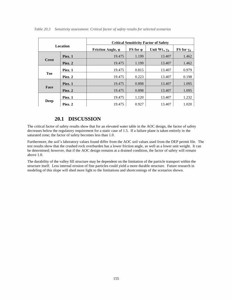
155
Table 20.3 Sensitivity assessment: Critical factor of safety results for selected scenarios
20.1 DISCUSSION
The critical factor of safety results show that for an elevated water table in the AOC design, the factor of safety
decreases below the regulatory requirement for a static case of 1.5. If a failure plane is taken entirely in the
saturated zone; the factor of safety becomes less than 1.0.
Furthermore, the soil’s laboratory values found differ from the AOC soil values used from the DEP permit file. The
test results show that the crushed rock overburden has a lower friction angle, as well as a lower unit weight. It can
be determined; however, that if the AOC design remains at a drained condition, the factor of safety will remain
above 1.0.
The durability of the valley fill structure may be dependent on the limitation of the particle transport within the
structure itself. Less internal erosion of fine particles could yield a more durable structure. Future research in
modeling of this slope will shed more light to the limitations and shortcomings of the scenarios shown.
Location Critical Sensitivity Factor of Safety
Friction Angle, φ FS for φ Unit Wt., γd FS for γd
Crest Piez. 1 19.475 1.199 13.407 1.462
Piez. 2 19.475 1.199 13.407 1.462
Toe Piez. 1 19.475 0.815 13.407 0.979
Piez. 2 19.475 0.223 13.407 0.198
Face Piez. 1 19.475 0.898 13.407 1.095
Piez. 2 19.475 0.898 13.407 1.095
Deep Piez. 1 19.475 1.120 13.407 1.232
Piez. 2 19.475 0.927 13.407 1.020

156
21. STABILITY ANALYSIS: GEOMORPHIC VALLEY FILL
ALTERNATIVE
Geomorphic design uses concepts derived from natural processes. Geomorphic landforms are designed with the
intent of emulating a naturally occurring landform whose erosion potential is minimized. The minimized erosion
potential is a function of drainage density. Drainage density is the ratio of the relationship between watershed area
per channel length.
Some initial benefits can be observed when addressing geomorphic landform design from a slope stability, and
earthen structure durability standpoint. Slope angles and lengths have the potential to be decreased. Smaller slopes
give water runoff shorter distances to travel before being collected in a drainage channel. This analysis was
performed to explore the stability capacity of the geomorphic landform design to be compared to the AOC valley fill
design with regard to a factor of safety computed from GeoStudio™ by the general limit equilibrium (GLE)
approach.
The geomorphic landform design shown in Figure 21.1 and Figure 21.2 below was produced with GeoFluv®
software. SLOPE/W was used for the slope stability analysis. The contours by which the profile dimensions were
retrieved are shown in Figure 21.1. The geomorphic alternative dimensions were retrieved from a centerline cut at
the identical dimensions as the valley fill centerline section A-A in Figure 19.2.
Figure 21.1 Geomorphic design contours superimposed on original ground contours

157
Figure 21.2 Geomorphic design surface generated from a triangulated irregular network (TIN)
Figure 21.3 Geomorphic valley fill alternative failure planes along centerline shown in Fig. 13.48

158
21.1 DATA INPUT PARAMETERS
The data that was input into the model to identify the geometry of the slope was taken from the AOC contours in
and the geomorphic design contours in Figure 21.1. The material’s geotechnical properties were input identically to
the data used for the AOC modeling in section 13.3 for accurate comparison. The failure planes were determines
such that the most critical areas would be analyzed. The critical areas were identified as the steepest areas along the
slope. From a slope stability standpoint, the steep slopes would have the highest driving forces for slope failure.
These areas should have the lowest factors of safety. Four locations were chosen for analysis as shown in Figure
21.3. Two piezometric scenarios were assessed separately. The piezometric lines were at a 10ft thickness along the
bottom of the fill to emulate a saturated gravity segregated durable rock underdrain, and a 50ft (15.24m) elevated
water table to emulate a more critical condition. Slope angles are shown in Table 25.1. Tables summarizing the
results of the deterministic and sensitivity factors of safety are shown below.
21.2 RESULTS
Table 21.1 Deterministic critical factors of safety for two piezometric scenarios
Laboratory Values
Location Critical Deterministic
Factor of Safety
Crest Piez. 1 1.816
Piez. 2 1.816
Toe Piez. 1 1.822
Piez. 2 1.616
Face Piez. 1 1.780
Piez. 2 1.780
Deep Piez. 1 1.944
Piez. 2 1.944
Table 21.2 Sensitivity critical factors of safety for two piezometric scenarios
Location Critical Sensitivity Factors of Safety
Friction Angle, φo
FS for φ Unit Wt., γd FS for γd FS
Crest Piez. 1 19.475 1.223 13.407 1.491 1.776
Piez. 2 19.475 1.223 13.407 1.491 1.776
Toe Piez. 1 19.475 1.227 13.407 1.497 1.783
Piez. 2 19.475 1.058 13.407 1.267 1.559
Face Piez. 1 19.475 1.199 13.407 1.462 1.741
Piez. 2 19.475 1.199 13.407 1.462 1.741
Deep Piez. 1 19.475 1.309 13.407 1.597 1.902
Piez. 2 19.475 1.309 13.407 1.597 1.902

159
22. CUMULATIVE ANALYSIS: AOC VALLEY FILL DESIGN
The modeling process undertaken for the valley fill under inspection in this section was for two scenarios. The first
scenario run was for the durable rock underdrain to be initially dry or unsaturated. The second condition run was for
the underdrain to be at an initially saturated state. The objective of the stability analysis performed for this valley
fill profile geometry was intended to imitate more realistic in-field conditions. SEEP/W was first used to produce
infiltration results over a 10 year period. The results from SEEP/W illustrated areas of storage, areas of increased
hydraulic head, and elevated pore pressures. The results from this analysis were utilized as parent inputs to a
SIGMA/W analysis. The SIGMA/W analysis, via finite element modeling techniques, calculated insitu stresses
within the fill structure. The insitu stresses varied from previous piezometric head conditions by having spatially
variable areas of increased total hydraulic head, as well as spatially variable areas of elevated pore pressures.
Finally, the SIGMA/W results were used as parent input parameters for the finite element SLOPE/W analysis. The
SLOPE/W analysis was run to produce factors of safety at several critical areas. The critical areas that were selected
for failure plane entry and exit points were chosen to be identical to the valley fill modeling shown in section 13.3
for comparison. Slope profile with cumulative analysis results shown in the following figures and tables.
Figure 22.1 Valley fill diagrams of results from a cumulative analysis of SEEP/W, SIGMA/W, and SLOPE/W
from GeoStudio™

160
Figure 22.2 Failure entry and exit locations for saturated underdrain – Deterministic analysis results
22.1 DATA INPUT PARAMETERS
The geometry of this valley fill profile was taken from the image in Figure 19.1. The geometry is identical to the
analysis described in section 13.3. The SEEP/W inputs are described in SEEP/W Analysis section in this chapter, or
section 13.1. The SIGMA/W input parameters are shown in Table 19.7. The blocky underdrain material had its
own unique hydraulic conductivity for the SEEP/W modeling, but had identical input parameters for strength, unit
weight, and friction angle as the fill material. The original ground material was considered as a weak sandstone with
an elastic modulus at the minimum for solid sandstone at 106 kPa.
22.2 RESULTS
Table 22.1 Deterministic factor of safety results: Saturated Underdrain
Laboratory Values Valley Fill - Saturated
Location Critical Deterministic
Factor of Safety
Crest 1.407
Toe 1.505
Face 1.389
Deep 1.375

161
Table 22.2 Deterministic factor of safety results: Unsaturated Underdrain
Laboratory Values Valley Fill - Unsaturated
Location Critical Deterministic
Factor of Safety
Crest 1.673
Toe 1.246
Face 1.365
Deep 1.299
Table 22.3 Sensitivity factor of safety results: Saturated Underdrain
Location Sensitivity FS: Valley Fill - Saturated
Friction Angle, φ Unit Wt., γd FS
Crest 19.475 13.407 1.377
Toe 19.475 13.407 1.472
Face 19.475 13.407 1.359
Deep 19.475 13.407 1.345
Table 22.4 Sensitivity factor of safety results: Unsaturated Underdrain
Location Sensitivity FS: Valley Fill - Unsaturated
Friction Angle, φ Unit Wt., γd FS
Crest 19.475 13.407 1.637
Toe 19.475 13.407 1.219
Face 19.475 13.407 1.335
Deep 19.475 13.407 1.271

162
23. CUMULATIVE ANALYSIS: GEOMORPHIC VALLEY FILL
ALTERNATIVE
The objective of the stability analysis performed for this geomorphic design valley fill alternative profile geometry
was intended to imitate more realistic in-field conditions than utilizing SLOPE/W alone. The modeling process
undertaken for the geomorphic design valley fill alternative under inspection in this section was for two scenarios.
The first scenario run was for the durable rock underdrain to be initially dry (unsaturated). The second condition run
was for the underdrain to initially be at a fully saturated state. The cumulative analysis procedure was identical to
the analysis run on the AOC valley fill design in the previous section (section 13.5), except for the failure plane
entry and exit selection. SEEP/W was first used to produce infiltration results over a 10 year period. The results
from SEEP/W illustrated areas of ground water storage, areas of increased hydraulic head, and elevated pore
pressures. The results from this analysis were utilized as parent inputs to a SIGMA/W analysis.
The SIGMA/W analysis, via finite element modeling techniques, calculated insitu stresses within the fill structure.
The insitu stresses varied from previous piezometric head conditions by having spatially variable areas of increased
total hydraulic head, as well as spatially variable areas of elevated pore pressures. Finally, the SIGMA/W results
were used as parent input parameters for the finite element SLOPE/W analysis. The SLOPE/W analysis was run to
produce factors of safety at several critical areas. The critical areas that were selected for failure plane entry and exit
points were chosen by considering areas where pore pressures were highest. Other failure plane entry and exit
locations were selected by keeping in mind general limit equilibrium concepts of driving forces and resisting forces
(or moments). The failure plane entry and exit location selection also involved keeping in mind the sometimes
significant effects that steep slope angles can have on the stability of an earthen structure. The slope profile with
cumulative analysis results are shown in the following figures and tables along with identified failure planes.
Figure 23.1shows output from (top to bottom) SLOPE/W, SIGMA/W, SEEP/W, then finally the finite element mesh
with a global element size of 10m. SEEP/W analysis was performed first to calculate the water storage through
hydraulic conductivity and water content functions. SIGMA/W was then utilized to calculate the insitu stresses
caused by the water storage and unit weight. SLOPE/W was lastly utilized to calculate factors of safety at three
critical locations.
Figure 23.1 Geomorphic valley fill alternative cumulative analysis results for unsaturated underdrain
conditions

163
23.1 DATA INPUT PARAMETERS
It is important to note that the profile geometry used for this model and the model described in section 13.4 vary
slightly. The reason for this alteration is that the original ground input dimensions varied in discretization between
the two illustrations in Figure 19.1 and Figure 21.1. Each geometry was chosen to be assessed in the manner laid
out in this chapter. The SEEP/W inputs are described in SEEP/W Analysis section in this chapter, or section 19.
The SIGMA/W input parameters are shown in Table 19.7. The blocky underdrain material had its own unique
hydraulic conductivity for the SEEP/W modeling, but had identical input parameters for strength, unit weight, and
friction angle as the fill material. The original ground material was considered as a weak sandstone with an elastic
modulus at the minimum for solid sandstone at 106 kPa.
23.2 RESULTS Table 23.1 Deterministic critical factor of safety results for the geomorphic design valley fill
alternative under an initial saturated underdrain condition
Laboratory Values
Geomorphic Design - Saturated
Location
Critical
Deterministic
FS
Crest 2.040
Toe 2.144
Face 2.242
Table 23.2 Sensitivity critical factor of safety results for the geomorphic design valley fill alternative
under an initial saturated undedrain condition
Sensitivity: Geomorphic Design - Saturated
Location Friction Angle, φ Unit Wt., γd FS
Crest 19.475 13.407 1.997
Toe 19.475 13.407 2.097
Face 19.475 13.407 2.194
Table 23.3 Deterministic critical factor of safety results for the geomorphic design valley fill
alternative under an initial unsaturated underdrain condition
Laboratory Values
Geomorphic Design - Unsaturated
Location
Critical
Deterministic
FS
Crest 2.309
Toe 3.491
Face 2.145

164
Table 23.4 Sensitivity critical factor of safety results for the geomorphic design valley fill alternative
under an initial unsaturated undedrain condition
Sensitivity: Geomorphic Design - Unsaturated
Location Friction Angle, φ Unit Wt., γd FS
Crest 19.475 13.407 2.260
Toe 19.475 13.407 3.416
Face 19.475 13.407 2.099
24. GEOMORPHIC DESIGN CRITICAL SLOPE ANALYSIS
This slope analysis was performed to illustrate areas of concern for the GeoFluv® geomorphic design process. The
geometry for these slopes were taken directly from the labeled location in the design in Figure 21.1. Since
GeoFluv® does not have a slope stability module or assessment of any kind to reinsure the durability of the output,
excessively steep slopes sometimes result. These excessively steep slopes result because the GeoFluv® program
bases the design on the hydraulic factors involving surface precipitation runoff. These hydraulic factors include
stream type, and stream slope. This particular slope was in a narrow part of the design. When inspecting Figure
21.1, one notices that the main channel and the design boundary are close to one another in proximity; however,
their individual elevations vary greatly. In response to this scenario, the design software “ties in” the two elevations
in a very short distance, producing a steep slope. Two piezometric conditions were modeled for this slope. The
results prove that this slope is too steep to meet the factor of safety requirement for AOC of 1.3. None of the 16
models that were run produced a factor of safety over 1.0. One promising insight is that within GeoFluv®, the
designer can mitigate these types of problems by changing the number of drainage channels, shifting the slope of the
drainage channel, or by altering cut and fill volumes in specific areas. Designer customization in any of these areas
will affect the calculated factor of safety. If a designer can identify critical slope areas accurately, then the low
factors of safety can be increased by altering the geometry of the landform. The factor of safety results are
presented in the tables below.
Figure 24.1 Critical slope profile with failure planes along centerline shown in Fig. 13.48. Pieziometric line
#2 enabled – Deterministic analysis visual results

165
24.1 DATA INPUT PARAMETERS
The geometry of the model, as noted above, was retrieved from the AutoCad™ output contours of the original
ground and the superimposed geomorphic design contours. The fill material and original ground material are
defined identical to the previous models. The material’s geotechnical properties were input according to Table 19.1-
Table 19.7. The failure planes were determined such that the most critical areas would be analyzed along the fill
surface. Two piezometric scenarios were assessed separately. The piezometric lines were at a 10ft thickness along
the bottom of the fill to model a saturated gravity segregated durable rock underdrain, and a 50ft (15.24m) elevated
water table to approximate a more critical condition. Tables summarizing the deterministic and sensitivity factors of
safety are shown below. Slope angles are shown in Table 25.1.
24.2 RESULTS
Table 24.1 Deterministic critical factor of safety results for the critical slope for two piezometric scenarios
Laboratory Values
Location Critical Deterministic
Factor of Safety
Crest Piez. 1 0.879
Piez. 2 0.879
Toe Piez. 1 0.409
Piez. 2 0.598
Face Piez. 1 0.685
Piez. 2 0.551
Deep Piez. 1 0.679
Piez. 2 0.535
Table 24.2 Sensitivity critical factor of safety results for the critical slope for two piezometric scenarios
Location Critical Sensitivity Factor of Safety
Friction Angle, φ FS for φ Unit Wt., γd FS for γd FS
Crest Piez. 1 19.475 0.611 13.407 0.745 0.887
Piez. 2 19.475 0.611 13.407 0.745 0.887
Toe Piez. 1 19.475 0.227 13.407 0.220 0.363
Piez. 2 19.475 0.402 13.407 0.489 0.584
Face Piez. 1 19.475 0.463 13.407 0.564 0.670
Piez. 2 19.475 0.345 13.407 0.400 0.519
Deep Piez. 1 19.475 0.468 13.407 0.570 0.677
Piez. 2 19.475 0.338 13.407 0.396 0.506

166
25. SUMMARY AND COMPARISON
Five separate assessments were performed in the modules available in GeoStudio™ for comparison. Through this
rigorous analysis, it was found that slope angles, phreatic elevations, and areas of increased pore pressures greatly
affected the factors of safety that were yielded by GeoStudio™ modules. The slope angles and associated
coordinates for each failure plane assessed are shown in the table below.
Table 25.1 Critical slip plane approximate exit point slope angles
Slope Angles
x (m) y (m) β
o=tan
-1(y/x)
Top Left Coord. Bottom Right Coord.
x (m) y (m) x (m) y (m)
Valley Fill 30.40 15.20 26.57 920.20 466.30 950.60 451.10
Geomorphic Alternative: Contour Profile
Face 19.81 4.57 12.99 383.88 208.79 403.69 204.22
Toe 25.05 4.57 10.34 950.76 103.63 975.81 99.06
Deep 22.62 4.58 11.45 403.69 204.22 426.31 199.64
Crest 18.96 4.57 13.55 349.49 217.93 368.45 213.36
Geomorphic Alternative: Plan Profile - Saturated
Face 16.52 4.57 15.47 813.90 435.86 830.42 431.29
Toe 14.39 4.57 17.63 1188.21 376.43 1202.60 371.86
Crest 22.62 4.57 11.43 403.689 509.02 426.31 504.44
Geomorphic Alternative: Plan Profile - Unsaturated
Face 35.48 4.57 7.34 904.86 417.58 940.33 413.00
Toe 68.09 4.57 3.84 975.82 403.86 1043.91 399.29
Crest 22.62 4.57 11.43 403.69 509.02 426.31 504.44
Geomorphic Critical Slope
Face 4.74 4.57 43.95 228.62 62.48 233.36 57.91
Toe 104.59 56.39 28.33 154.45 91.44 259.04 35.05
Deep 6.48 4.57 35.19 252.56 39.62 259.04 35.05
Crest 5.82 4.57 38.14 172.3 108.2 178.12 103.63
The height of the piezometric line had a profound influence on the factors of safety. When an area was saturated,
the factor of safety decreased, sometimes below 1.0 as in the piez. 2 toe scenario of the AOC valley fill design
(Table 25.2). If the piezometric line was not elevated to the area of the selected failure plane, then the factor of
safety remained unchanged. Additionally, steeper slope angles decreased factors of safety. Two initial saturation
conditions were modeled for the cumulative analysis. The saturation conditions were applied in SEEP/W, and
SIGMA/W computed in situ stresses to be input into SLOPE/W for a factor of safety computation. The initial
saturation condition of the gravity segregated durable rock underdrain was significant. The initial saturation altered
the volume of water retained within the structure, and ultimately altered the factors of safety that resulted. Table
25.1 and Table 25.2 show the factors of safety for both the saturated and unsaturated initial hydraulic condition. The
factors of safety vary from one hydraulic condition to the next, but do not necessarily increase or decrease
accordingly. The result is an effect of the varying areas of increased pore pressure. The result of the SEEP/W
analysis produced outputs that accumulated water storage within each fill in different areas, which resulted in
varying factors of safety. Both cumulative analysis that were run for the geomorphic design and the valley fill
proved that the initial condition could vary the factor of safety. The change in the factor of safety was not always in
favor of either condition from a structural standpoint. The significance of the initial saturation condition was that

167
the water storage areas within the fill changed, and altered the factors of safety. It is important to note that the fills
may be built in lifts or by end dumping. Sometimes when contractors build slopes, they cut into the original ground,
and may use compaction equipment to help integrate the components of the structure. These considerations would
likely alter the factors of safety. Additionally, spatial variability was only taken into account in these models as a
sensitivity analysis. Field conditions of a slope structure would have a great deal of spatial variability both in
compaction and in initial water content affecting soil strength and phreatic surface elevations.
By far, the cumulative analysis for the geomorphic valley fill alternative design yielded the highest factors of safety.
Most cases produced factors of safety over 2.0. The most likely reason for these high factors of safety is that the
geomorphic design has shallower slopes, and drains well. Geomorphic landform design can be utilized to reduce
infiltration volumes by shortening runoff travel distances, increasing runoff water removal from a design site. A
completed design should retain less water than the modeled results show because of vegetative cover and quick
surface runoff. Both initial saturated and unsaturated conditions yielded high factors of safety. The failure locations
were sought out to find the lowest factors of safety for the structure. The geomorphic stability analysis described in
section 13.4 yielded high factors of safety (Table 25.3) also; however, the water tables were exaggerated. The
profile described in section 13.4 still retains its structural integrity even when high volumes of water are being stored
within it. None of the factors of safety even under the most critical circumstances tested yielded factors of safety
under 1.0. Even though the original ground dimensions vary for the two profiles, the surface dimensions are
identical except for the near the toe. The results prove that the geomorphic design can remain very stable under
different conditions and geometries.
The weakest structure was by far the critical slope described in section 24. None of the factors of safety under any
scenario analyzed yielded a factor of safety over 1.0. The factors of safety of this structure were expected to be low.
The analysis of the critical slope was intended to illustrate that GeoFluv® does not consider slope stability, and can
produce slopes that are not stable. As discussed in section 13.7, GeoFluv® does enable the designer to alter many
components of the design to mitigate the slope stability problems that may occur due to rapid elevation changes.
The AOC design was typical with its bench cuts and planar slopes. Regulations require that slope factors of safety
must remain above 1.3. The analysis performed showed that the design could withstand insitu loads and slope angle
under most conditions analyzed. Elevated pore pressures tended to result at the toe of the slope, and decreased the
factor of safety. The most critical scenario was a totally saturated toe which yielded a factor of safety of 0.50 as
shown in the piez. 2 toe AOC valley fill design model summary in Table 25.1.
The SEEP/W analysis yielded results that implied that the structure drained well for the AOC valley fill design.
There were small areas of water storage accumulation and elevated pore water pressures, but nothing which caused
the factor of safety to drop below 1.0 for the cumulative analysis. For the cumulative analysis, the lowest factor of
safety for the AOC valley fill design was 1.22 at the toe of the slope at an initially unsaturated durable rock
underdrain condition.
Geomorphic design decreases erosion potential and therefore decreases maintenance demands. The proposed AOC
design would be adequate if it remained sufficiently drained. If particle transport can occur and alter toe pore
pressures, it is possible that some small slope failure may occur. The gradations that were found in the fill material
in Chapter 9 and Chapter 12 show that particle transport probably would not be a concern for the laboratory tested
unweathered sandstone.

168
Table 25.2 AOC valley fill slope summary
Slope Angles and Correlating Factors of Safety
Failure
Plane
Hydraulic
Condition β
o=tan
-1(y/x)
Critical
Deterministic Factor
of Safety
Critical Sensitivity
Factor of Safety
AOC Valley Fill Design (Permit Values)
Crest
Piez. 1 26.57 2.84 -
Piez. 2 26.57 2.84 -
Toe
Piez. 1 26.57 1.51 -
Piez. 2 26.57 0.91 -
Face
Piez. 1 26.57 2.13 -
Piez. 2 26.57 2.13 -
Deep
Piez. 1 26.57 1.54 -
Piez. 2 26.57 1.41 -
AOC Valley Fill Design (Laboratory Values)
Face Piez. 1 26.57 1.78 1.74
Piez. 2 26.57 1.78 1.74
Toe Piez. 1 26.57 1.23 1.20
Piez. 2 26.57 0.50 0.40
Deep Piez. 1 26.57 1.33 1.31
Piez. 2 26.57 1.33 1.31
Crest Piez. 1 26.57 1.37 1.35
Piez. 2 26.57 1.21 1.18
Cumulative Analysis: AOC Valley Fill Design - Saturated
Crest Saturated 26.57 1.41 1.38
Toe Saturated 26.57 1.51 1.47
Face Saturated 26.57 1.39 1.36
Deep Saturated 26.57 1.38 1.35
Cumulative Analysis: AOC Valley Fill Design - Unsaturated
Crest Unsaturated 26.57 1.67 1.64
Toe Unsaturated 26.57 1.25 1.22
Face Unsaturated 26.57 1.37 1.34
Deep Unsaturated 26.57 1.30 1.27

169
Table 25.3 Geomorphic valley fill alternative slope summary
Slope Angles and Correlating Factors of Safety
Failure
Plane
Hydraulic
Condition β
o=tan
-1(y/x)
Critical
Deterministic
Factor of Safety
Critical Sensitivity
Factor of Safety
Stability Analysis: Geomorphic Valley Fill Alternative
Face Piez. 1 12.99 1.82 1.78
Piez. 2 12.99 1.82 1.78
Toe Piez. 1 10.34 1.82 1.78
Piez. 2 10.34 1.62 1.56
Deep Piez. 1 11.45 1.78 1.74
Piez. 2 11.45 1.78 1.74
Crest Piez. 1 13.55 1.94 1.90
Piez. 2 13.55 1.94 1.90
Cumulative Analysis: Geomorphic Valley Fill Alternative - Saturated
Crest Saturated 11.43 2.04 2.00
Toe Saturated 17.63 2.14 2.10
Face Saturated 15.47 2.42 2.19
Cumulative Analysis: Geomorphic Valley Fill Alternative - Unsaturated
Crest Unsaturated 11.43 2.31 2.26
Toe Unsaturated 3.84 3.49 3.42
Face Unsaturated 7.34 2.15 2.10
Geomorphic Critical Slope
Face Piez. 1 43.95 0.88 0.89
Piez. 2 43.95 0.88 0.89
Toe Piez. 1 28.33 0.41 0.36
Piez. 2 28.33 0.60 0.58
Deep Piez. 1 35.19 0.69 0.67
Piez. 2 35.19 0.55 0.52
Crest Piez. 1 38.14 0.68 0.68
Piez. 2 38.14 0.54 0.51

170
26. CONCLUSIONS AND PRACTICAL SIGNIFICANCE
Soil Testing and Stability Analysis
The objective of this research was to sample and identify a surface mine spoil in southern West Virginia,
characterize its associated physical properties as well as the strength aspects for appropriate input parameter key in
into a slope stability software analysis tool to compare stability results of an AOC valley fill and a geomorphic
landform design with regard to a factor of safety computed by the general limit equilibrium method. The significant
conclusions of this research are as follows:
By rigorous analysis of the laboratory testing for the unweathered sandstone overburden material, the following
conclusions were identified:
The standard proctor curve is a typical bell shaped curve with an optimum dry unit weight of 18.75 kN/m3 at a
moisture content of approximately 10.75%. The 34% proctor curve resembles a transition between standard
proctor and 11% proctor curves. The optimum dry density of the 34% proctor curve was 18.1 kN/m3 at a
moisture content of 14.50%. The 11% proctor curve shows a compaction curve resembling a standard behavior
for a well graded sand. The optimum dry density of the 11% proctor was at 17.6 kN/m3 with a moisture content
of approximately 17.00%. The minimum dry density of the 11% curve was at 10.50% moisture content at a
value of 14.90 kN/m3. The compaction energy applied in these three scenarios varied from 592.5 kJ/m
3
(standard proctor), 203.6 kJ/m3(
34% proctor), and 67.85 kJ/m
3 (11% proctor). The optimum dry densities did
not increase by much, only a difference of 1.15 kN/m3 between standard proctor and 11% proctor compaction.
The corresponding moisture contents for these maximums varied from 10.75% (standard proctor) to 17.00%
(11% proctor) at a difference of 6.25%. By observation of the data, the material does not need a significant
amount of compaction in order to achieve a high dry density, but it does need the accompanying moisture
content to achieve it.
The shear strain curves revealed that much of the residual strength is retained within the sample. The reason the
samples retained their strength is likely a result of the creation of the unweathered material. The geometry of
the particles of the sample is angular. The material was blasted, unweathered rock. The angular nature of the
material increases the friction between shear planes and resists displacement. This insight is beneficial when
considering slope stability. Slopes constructed with this material should be strong and resistant to failure
(FS<1). Regulations require a factor of safety of 1.3 or greater.
The hydraulic conductivity for each test performed for standard proctor, 34% proctor, and 11% proctor all
remained in the order of 10-9
m/s. The neither the 34% proctor permeated specimens, nor the standard proctor
specimens had hydraulic consolidation effects. Some hydraulic consolidation did occur for the 11% proctor
specimens. The consolidation that occurred was the cause of the low hydraulic conductivity of the 11% proctor
specimens. The soil structure could not retain its skeleton and void spaces collapsed under the hydraulic
gradient of i=15. The standard proctor and 34% proctor specimens had low porosities in a range of n=0.31 to
n=0.38 which resulted in low hydraulic conductivities.
While observing the summary of the gradations produced by the as received grain size distribution, the pre-
permeability test specimens, and the post-permeability specimens, the following conclusions were formed:
Comparatively, taking into consideration all three compaction energies and the results shown above of the test
scenarios performed it was found that particle movement varied significantly. The variation in gradation was a
function of the moisture content added and the energy applied for preparation. The post-permeability results
should be interpreted carefully as each specimen of different density varied in pore volume flux. The standard
proctor specimens aggregated the most between D50 and D15 due to compaction, then aggregated more at a post-
permeability condition. The 34% Proctor compaction specimens showed similar results as standard proctor,
aggregating more at a post-permeability condition. The 11% Proctor compaction specimen results were
opposite 34% Proctor compaction results and standard proctor compaction results. The 11% Proctor
compaction specimen aggregated most at a pre-permeability condition, then became less aggregated at a post-
permeability condition.
The results of the particle transport analysis indicate that the unweathered sandstone material reaches an
aggregated equilibrium with very similar gradation after some pore volumes of water permeate through it. The

171
results also imply that introducing a range of compaction energy can alter soil properties and have performance
implications on earthen structures. Layered construction known as “lift construction” could assist in better
quality control of the compaction energy applies to earthen structures to more precisely manage the aggregation
phenomena. The amount of compaction energy for the 34% Proctor compaction and standard proctor samples
seems to have broken up the aggregated particles, then when they were permeated, became more aggregated.
After the permeation occurred, all three compaction energies approached a similar gradation, but diverged
somewhat as the particle size decreased. The specimens began diverging in similarity around 40% finer.
Through rigorous grain size distribution analysis of the pre and post-permeability test specimens, it was found
that at a D10 post-permeability condition, the 11% Proctor compaction energy compacted and permeated sample
had the smallest particles, standard proctor had the next highest, and 34% Proctor energy specimens had the
largest particle size. Overall the 11% proctor pre-permeability condition had the most aggregated particles,
likely due to little compaction energy applied to break apart aggregated particles. At D10 at a pre-permeability
condition, the standard proctor sample had the smallest particles, then 34% proctor, and 11% Proctor energy
samples had the largest aggregated particles.
The numerical modeling of the AOC valley fill design juxtaposed with the geomorphic landform design alternative,
the following significant conclusions were drawn:
The height of the piezometric line had a profound influence on the factors of safety. When an area was
saturated, the factor of safety decreased, sometimes below 1.0 as in the piez. 2 toe scenario of the AOC valley
fill design (Table 25.1). If the piezometric line was not elevated to the area of the selected failure plane, then
the factor of safety remained unchanged. Steep slope angles also decreased the factors of safety
Two initial saturation conditions were modeled for the cumulative analysis. The saturation conditions were
applied in SEEP/W, and SIGMA/W computed insitu stresses to be input into SLOPE/W for a factor of safety
computation. The initial saturation condition of the gravity segregated durable rock underdrain was significant.
The initial saturation condition altered the volume of water retained within the structure, and ultimately altered
the factors of safety that resulted.
In the cumulative analysis, the change in the factor of safety was not always in favor of either saturation
condition from a structural standpoint. The significance of the initial saturation condition was that the water
storage areas within the fill changed, and altered the factors of safety. It is important to note that the fills may
be built in lifts or by end dumping. Sometimes when contractors build slopes, they cut into the original ground,
and may use compaction equipment to help integrate the components of the structure. These considerations
would likely alter the factors of safety.
The cumulative analysis for the geomorphic valley fill alternative design yielded the highest factors of safety.
Most cases produced factors of safety over 2.0. The most likely reason for these high factors of safety is that
the geomorphic design has shallower slopes, and drains well. Geomorphic landform design can be utilized to
reduce infiltration volumes by shortening runoff travel distances, increasing runoff water removal from a design
site. A completed design should retain less water than the modeled results show because of vegetative cover
and quick surface runoff.
The geomorphic stability analysis described in section 13.4 yielded high factors of safety between 1.56 and 1.92
(Table 25.2) also; however, the water tables were exaggerated. The geomorphic profile described in section
13.4 still retains its structural integrity even when high volumes of water are being stored within it. None of the
factors of safety even under the most critical circumstances tested yielded factors of safety under 1.0. The
results prove that the geomorphic design can remain stable under extreme hydraulic conditions and varying
geometries.
The weakest structure assessed was by far the critical slope described in section 13.7. None of the factors of
safety under any scenario analyzed yielded a factor of safety over 1.0. The factors of safety of this structure
were expected to be low. The analysis of the critical slope was intended to illustrate that GeoFluv® does not
consider slope stability, and can produce slopes that are not stable. As discussed in section 13.7, GeoFluv®
does enable the designer to alter many components of the design to mitigate the slope stability problems that
may occur due to rapid elevation changes.
The analysis performed for the AOC valley fill design showed that the design could withstand insitu loads and
slope angle under most conditions analyzed. Elevated pore pressures tended to result at the toe of the slope, and

172
decreased the factor of safety. The most critical scenario was a totally saturated toe which yielded a factor of
safety of 0.50 as shown in the piez. 2 toe AOC valley fill design model summary in Table 25.1.
In the cumulative analysis, the SEEP/W assessment yielded results that implied that the structure drained well
for the AOC valley fill design. There were small areas of water storage accumulation and elevated pore water
pressures, but nothing which caused the factor of safety to drop below 1.0. For the cumulative analysis, the
lowest factor of safety for the AOC valley fill design was 1.22 at the toe of the slope at an initially unsaturated
durable rock underdrain condition.
The conclusions pointed to supporting the idea of the geomorphic design of valley fills having advantages over
Approximate Original Contour design applied to valley fills from a slope stability perspective.
A geomorphic fill showed a distinct advantage in the durability of the earthen structure geometry addressed. To
further analyze the comparison between a geomorphic and AOC fill, probabilistic analyses could be performed to
more thoroughly account for spatial variability. Spatial variability was only taken into account in these models as a
sensitivity analysis. Field conditions of a slope structure would have a great deal of spatial variability both in
compaction and in initial water content affecting soil strength and phreatic surface elevations.
The AOC valley fill design would be adequate if it remained sufficiently drained. If particle transport can occur and
alter toe pore pressures, it is possible that some small slope failure may occur. The gradations that were found in the
fill material in Chapter 9 and Chapter 12 show that particle transport probably would not be a concern for the
laboratory tested unweathered sandstone.
Geomorphic design decreases erosion potential and therefore decreases maintenance demands theoretically,
however, in order to fully address this potential benefit of geomorphic landform design, a thorough cost analysis
with regard to construction techniques in AOC and geomorphic landform design would need to be investigated.
SEEP/W Analysis
By analyzing each fill individually, collecting results, and comparing those results, conclusions about the
comparison of an AOC fill and geomorphic fill were collected. When looking at the comparison of results between
the two fills, the conclusions were as follows:
For both the AOC and geomorphic fill, the majority of flow was both within the drain and in the saturated
zone above the drain. Water within the drain caused a negative pore-pressure above the drain. This was
because the drain was modeled in a saturated only condition. The drain was saturated for the entire
duration of the model, so for this reason, the soil retained a saturated zone above the drain. As the zone
between the drain and the saturated zone drained, negative pore pressure kept the saturated zone in tension
and at a level above the drain. Over time, the level of saturation lowers towards the level of the drain.
The range of pore-water pressure values for the two fills was almost equal. This is because the geomorphic
fill did not alter the soil properties, so the same range of pore-water pressures occurred. For each fill, the
fill material had the same soil-water characteristic curve, so the behavior of pore-water pressure over time
was the same.
The water velocity of the toe was lower for the AOC fill than for geomorphic fill for every year of the 10
year model except for year 9. Water velocity at the toe showed an advantage for the geomorphic fill for
the entire duration other than a short time in year 9, where the AOC fill had a 98.2% advantage. The
geomorphic fill had peaks in advantage of 1291.1% at year 3 and 1646.6% at year 7.
Year 5 showed a spike in the flux of the AOC fill, whereas the flux of the geomorphic fill stayed at a more
stable rate through years 3 through 10. The AOC fill has an advantage over the geomorphic fill from years
1-2, 4-6, and 8.5-9.5 with peaks in its advantage of 76.0% at year 5 and 100.0% at year 9. The geomorphic
fill is advantageous from years 2-4, 6-8.5, and 9.5-10 with its peaks in advantage of 405.4% at year 3 and
1141.7% at year 7.
Year 5 showed a spike in the velocity of the AOC fill, whereas the flux of the geomorphic fill stayed at a
more stable rate through years 3 through 10. The AOC fill had an advantage over the geomorphic fill from
years 1-2, 4-6, and at a very short time during year 9. The peak advantages for the AOC fill were 73.6% at
year 5 and 28.2% at year 9. The geomorphic fill was advantageous from years 2-4 and 6-10 with peaks in
advantage of 482.1% at year 3 and 1273.7% at year 7.

173
The geomorphic fill shows a much steadier and smoother increase in storage percentage over time. The
geomorphic fill had an advantage for the duration of the 10 years except between years 3 and 4, where the
AOC fill showed an advantage of 3.2%. The peaks in advantage for the geomorphic fill was 24.3% in year
6. The magnitude of the advantage for the AOC fill between years 3 and 4 was much lower than the
advantage for the geomorphic fill for all the other years.
For water velocity at the toe, water flux at the toe, maximum hydraulic velocity, and storage, the magnitude
of the geomorphic fill’s advantage was much higher than the advantage for the AOC fill. The advantage
was a result of the geomorphic fill moving water through the fill at a faster rate.
When looking at the summary of the percent changes from the AOC fill to geomorphic fill, the following
conclusions were made:
In every category, the geomorphic fill showed an advantage for the majority of the time steps.
The greatest advantage was seen in the velocity at the toe. The next highest advantage was seen in water
flux at the toe and maximum hydraulic velocity.
Storage showed an advantage for the geomorphic fill for the majority of the model, but with a lower
magnitude of advantage.
If the percent differences for each criterion and each time step were totaled, it was seen that the geomorphic
fill had an overall advantage throughout the entire 10 year model.
Finally, a comparison of the slope stability results provided the following conclusions:
For all failure modes, both the AOC fill and geomorphic fill had a factor of safety greater than the valley
fill design standard of 1.3.
The geomorphic fill, however, had a higher factor of safety in each case. Almost all factors of safety were
above 2.0, whereas the factors of safety for the AOC fill ranged from 1.3-1.5. This was a result of the
geomorphic fill having a less steep slope and draining better than the AOC fill, producing less stress from
seepage.
All of these conclusions pointed to supporting the idea of the geomorphic design of valley fills having advantages
over Approximate Original Contour design.
A geomorphic fill showed a distinct advantage in the behavior of groundwater seepage. To further analyze the
comparison between a geomorphic and AOC fill, these groundwater seepage results could be applied to contaminant
transport. Selenium is a naturally present trace metal that at high concentrations can be toxic to humans and
ecosystems and can be released during mining. It is present in coal overburden and waste. Selenium enters ground
and surface water by being desorbed from coal waste by water. The geomorphic fill’s advantage with regards to
seepage could translate into an advantage in contaminant transport. Since the geomorphic fill stores less water and
moves water through the fill at a faster rate, there is less contact time with waste rocks to desorb the selenium. This
is something that would have to be investigated further using the CTRAN/W module of GeoStudio to model the
contaminant transport. Another area that needs to be investigated to fully compare the differing design techniques is
the construction and lifetime cost of implementing a geomorphic fill versus an AOC fill. Also, a longer time
period could be analyzed in order to further compare the behavior of groundwater in the AOC and geomorphic fills.
With the very limited amount of work that has been done with geomorphic fills in the region of central Appalachia,
this research has provided a sound initial analysis to compare with previously used design techniques. Further
research must be done in order to make a fully informed decision as to whether or not geomorphic design would be
feasible to implement in the reclamation of surface mines in central Appalachia.

174
References
Abdelghani, F.B., Simon, R., Aubertin, M, Molson, J. & Therrien, R. (2009). “Use of the hydrogeosphere code to
simulate water flow and contaminants transport through mining wastes disposed in a symmetric open pit
within fractured rock.” Proc. Tailings and Mine Waste. Taylor and Francis Group. Vail, CO. 601-611.
Akan, A.O. (1993). “Losses from rainfall.” Urban stormwater hydrology: a guide to engineering calculations.
Lancaster, PA. Technomic Publishing Co., Inc, 33.
ASTM Designation D422. (2007). “Standard Test Method for Particle-Size Analysis of Soils.” Annual Book of
ASTM Standards, American Society of Testing Materials, Easton, MD.
ASTM Designation D698. (2007). “Standard Test Methods for Laboratory Compaction Characteristics of Soil Using
Standard Effort (12400 ft-lbf/ft3 (600 KN-m/m
3)).” Annual Book of ASTM Standards, American Society of
Testing Materials, Easton, MD.
ASTM Designation D854. (2007). “Standard Test Methods for Specific Gravity of Soil Solids by Water
Pycnometer.” Annual Book of ASTM Standards, American Society of Testing Materials, Easton, MD.
ASTM Designation D2216. (2007). “Standard Test Methods for Laboratory Determination of Water (Moisture)
Content of Soil and Rock by Mass.” Annual Book of ASTM Standards, American Society of Testing
Materials, Easton, MD.
ASTM Designation D2487. (2010). “Standard Practice for Classification of Soils for Engineering Purposes (Unified
Soil Classification System).” Annual Book of ASTM Standards, American Society of Testing Materials,
Easton, MD.
ASTM Designation D3080. (2007). “Standard Test Methods for.Direct Shear Test of Soils Under Consolidated
Drained Conditions.” Annual Book of ASTM Standards, American Society of Testing Materials, Easton,
MD
ASTM Designation D4318. (2007). “Standard Test Methods for Liquid Limit, Plastic Limit, and Plasticity Index of
Soils.” Annual Book of ASTM Standards, American Society of Testing Materials, Easton, MD
ASTM Designation D-5856. (2007). “Standard test Method for Measurement of Hydraulic Conductivity of Porous
Material using a Rigid-Wall, Compaction-Mold Permeameter.” Annual Book of ASTM Standards,
American Society of Testing Materials, Easton, MD.
Aubertin, M., Bussierre, B. & Chapuis, R. (1996). “Hydraulic conductivity of homogenized tailings from hard rock
mines.” Can. Geotech. J., 33: 470-482.
Bedient, P.H., Huber, W.C. & Vieux, B.E. (2008). “Hydrologic principles.” Hydrology and floodplain analysis, 4th
ed. M.J. Horton, ed., Prentice-Hall Inc., Upper Saddle River, NJ, 65.
Bell, J.C., Daniels, W.L., and Zipper, C.E. 1989. The practice of “approximate original contour” in the central
Appalachians. I. Slope stability and erosion potential. Landscape Urban Plann., 18, 127-138.
Bugosh, N. 2004. Computerizing the fluvial geomorphic approach to land reclamation. National Meeting of the
American Society of Mining and Reclamation and The 25th West Virginia Surface Mine Drainage Task
Force, April 18-24, 240-258.
Bugosh N. 2009. A summary of some land surface and water quality monitoring results for constructed GeoFluv®
landforms. Revitalizing the Environment: Proven Solutions and Innovative Approaches, National Meeting
of the American Society of Mining and Reclamation, Billings, MT, May 30 – June 5, 153-175.
Das, Braja M. (2006). Principles of Geotechnical Engineering (7th
ed.). Canada: Nelson Education Ltd.
Davis ED, Duffy RJ. 2009. King coal vs. reclamation: Federal regulation of mountaintop removal mining in
Appalachia. Administration and Society, 41(6), 674692.
Deissmann, G., Goldsworthy, M., Kistinger, S., Stollenwerk, R.H. & Systemplanung, B. “Design constraints on
engineered dry covers for waste rock dumps.”

175
Eckels, R, Bugosh N. 2010. Natural approach to mined land reclamation. FIG Congress 2010.
Ferrari JR, Lookingbill TR, McCormick B, Townsend PA. 2009. Surface mining and reclamation effects on flood
response of watersheds in the central Appalachian Plateau region. Water Resources Research, 45,
W04407.
Fredlund, M.D., Wilson, G.W. & Fredlund, D.G. (1998). “Estimation of hydraulic properties of an unsaturated soil
using a knowledge-based system.” Proc., Second Inter. Conf. on Unsat. Soils. Beiling, China.
GEO-SLOPE International Ltd. (2007). Stability Modeling with SLOPE/W 2007 Version. Calgary, Alberta, Canada.
H. Gercek. April 22, 2006. “Poisson’s ratio values for rocks.” Elsevier. International Journal of Rock Mechanics &
Mining Sciences 44 (2007) 1-13.
Hartman KJ, Kaller MD, Howell JW, Sweka JA. 2005. How much do valley fills influence headwater streams?
Hydrobiologia, 532, 91-102.
Hasselman, M. 2002. Bragg v. W-Va. Coal Ass’n and the unfortunate limitation of citizen suits against the state in
cooperative federalism regimes. Ecol. Law Quart. 29: 205-229.
Huber, W.C. & R.E. Dickinson. (1998). Storm Sewer Management Model, Version 4, User’s Manual.
Environmental Research Laboratory, Athens, GA. U.S. Environmental Protection Agency.
Martin-Duque JF, Sanz MA, Bodoque JM, Lucia A, Martin-Moreno C. 2009. Restoring earth surface processes
through landform design. A 13-year monitoring of a geomorphic reclamation model for quarries on slopes.
Earth Surface Processes and Landforms, 35, 531-548.
Martin-Moreno C, Martin-Duque JF, Nicolau JM, Sanchez L, Ruiz R, Sanz MA, Lucia A, Zapico I. 2008. A
geomorphic approach for the ecological restoration of kaolin mines at the Upper Tagus Natural Park
(Spain). 6th
European Conference on Ecological Restoration, Ghent, Belgium, August 8-12.
Measles D., Bugosh N. 2007. Making and building a fluvial geomorphic reclamation design at an active dragline
mine using the GeoFluv® design method. 30 Years of SMCRA and Beyond, National Meeting of the
American Society of Mining and Reclamation, Gillette, WY, June 2-7, 2007, 449-456.
Meek, A. & O’dell, K. (2012). “Selenium Treatment Arch-Eastern, Birch Mine.” Proc., West Virginia Mine
Drainage Task Force Symposium. Morgantown, WV.
Michael PR, Superfesky MJ, Uranowski LJ. 2010. “Challenges to applying the geomorphic and stream reclamation
methodologies to mountaintop mining and excess spoil fill construction in steep-slope topography (e.g.
Central Appalachia).” 2010 National Meeting of the American Society of Mining and Reclamation,
Pittsburgh, PA Bridging Reclamation, Science and the Community June 5 - 11, 2010. R.I. Barnhisel (Ed.)
Published by ASMR, 3134 Montavesta Rd., Lexington, KY 40502.
National Oceanic and Atmospheric Administration. (2012). “Precipitation Frequency Data Server (PFDS).”
Hydrometeorological Design Studies Center, <http://hdsc.nws.noaa.gov> (Feb. 10, 2012).
Palmer, M.A., Bernhardt, E.S., Schlesinger, W.H., Eshleman, K.N., Foufoula-Georgiou, E., Hendryx, M.S., Lemly,
A.D., Likens, G.E., Loucks, O.L., Power, M.E., White, P.S. & Wilcock, P.R. (2010). “Mountaintop mining
consequences.” Science. 327, 148-149.
Pitt, R., Chen, S. & Clark, S. (2001). “Infiltration through compacted urban soils and effects on biofiltration design.”
Proc., Low Impact Development Roundtable Conference. Baltimore, MD.
Pond GJ, Passmore ME, Borsuk FA, Reynolds L, Rose CJ. 2008. Downstream effects of mountaintop coal mining:
comparing biological conditions using family- and genus-level macroinvertebrate bioassessment tools. J.
N. Am. Benthol. Soc., 27(3), 717-737.
Robson M, Spotts R, Wade R, Erickson W. 2009. A case history: Limestone quarry reclamation using fluvial
geomorphic design techniques.
Rosgen DL. 1994. A classification of natural rivers. Catena, 22, 169-199.
Rosgen, D. 1996. Applied River Morphology. Wildland Hydrology, Pagosa Springs, Colorado.

176
Sharma, K.D., Singh, H.P. & Pareek, P. (1983). “Rainwater infiltration into a bare loamy sand.” Hydrological Sci.
J., 28(3), 417-424.
Superfesky, M., Michael P. (2007). “Excess Spoil Minimization and Fill Stability.” Proc., SME Annual Meeting,
SME, Denver, CO, 1-13.
Toy TJ, Chuse WR. 2005. “ Topographic reconstruction: a geomorphic approach.” Ecological Engineering, 24, 29-
35.
USEPA. 2005. Final Programmatic Environmental Impact Statement (PEIS) on Mountaintop Mining/Valley Fills in
Appalachia (EPA 9-03-R-05002). U.S. Environmental Protection Agency.
http://www.epa.gov/region03/mtntop/eis2005.htm
Vesper, D.J., Roy, M., Rhoads, C.J. (2007). Selenium distribution and mode of occurrence in the Kanawka
Formation, southern West Virginia, U.S.A. Int. J. Coal Geol., 73(3), 237-249.
West Virginia Department of Environmental Protection, Division of Mining and Reclamation. (1999). Permit
Handbook: AOC and excess spoil disposal.
West Virginia Department of Environmental Protection (WVDEP), Permit ID S500809. Pine Creek No. 2 Surface
Mine (July 12, 2007).
Ziemkiewicz, P.F. & Lovett, R.J. (2011). “Determination of natural attenuation of selenium at a coal-mining
complex in West Virginia.”
Ziemkiewicz, P., O'Neal, M., and Lovett, R. (2011). Selenium leaching kinetics and in-situ control. Mine Water &
the Environment, 30(2), 141-150.

177
Appendices
Appendix I - Hydraulic Conductivity Data Tables
Hydraulic Conductivity: Test 1 – Standard Proctor Compaction (592.5 kJ/m3)
Time Vol (ml) Δt (min) Time
(Seconds) Δt
Cumulative
(Seconds) Δt
Time (Hours) Δt (hours)
Cumulative
12/21/11 3:00 PM 0 0 0 0 0 0
1/3/11 12:45 PM 0 0 0 0 0 0
1/5/12 10:16 AM 0 21316 1278960 1278960 355.27 355.27
1/5/12 10:25 AM 30 21325 540 1279500 355.42 0.15
1/5/12 10:33 AM 50 21333 480 1279980 355.55 0.13
1/5/12 10:46 AM 70 21346 780 1280760 355.77 0.22
1/5/12 11:05 AM 95 21365 1140 1281900 356.08 0.32
1/5/12 11:20 AM 115 21380 900 1282800 356.33 0.25
1/5/12 11:35 AM 130 21395 900 1283700 356.58 0.25
1/5/12 11:50 AM 145 21410 900 1284600 356.83 0.25
1/5/12 12:05 PM 160 21425 900 1285500 357.08 0.25
1/5/12 12:20 PM 175 21440 900 1286400 357.33 0.25
1/5/12 12:35 PM 190 21455 900 1287300 357.58 0.25
1/5/12 12:50 PM 200 21470 900 1288200 357.83 0.25
1/5/12 1:05 PM 215 21485 900 1289100 358.08 0.25
1/5/12 1:20 PM 225 21500 900 1290000 358.33 0.25
1/5/12 1:35 PM 235 21515 900 1290900 358.58 0.25
1/5/12 1:50 PM 250 21530 900 1291800 358.83 0.25
1/5/12 2:05 PM 260 21545 900 1292700 359.08 0.25
1/5/12 2:20 PM 270 21560 900 1293600 359.33 0.25
1/5/12 2:40 PM 280 21580 1200 1294800 359.67 0.33
1/5/12 3:00 PM 295 21600 1200 1296000 360.00 0.33
1/5/12 3:30 PM 315 21630 1800 1297800 360.50 0.50
1/5/12 4:00 PM 335 21660 1800 1299600 361.00 0.50
1/5/12 4:30 PM 350 21690 1800 1301400 361.50 0.50
1/5/12 5:00 PM 370 21720 1800 1303200 362.00 0.50
1/5/12 5:30 PM 385 21750 1800 1305000 362.50 0.50
1/5/12 6:00 PM 400 21780 1800 1306800 363.00 0.50
1/5/12 6:30 PM 415 21810 1800 1308600 363.50 0.50
1/5/12 7:00 PM 430 21840 1800 1310400 364.00 0.50
1/5/12 8:53 PM 490 21953 6780 1317180 365.88 1.88
1/5/12 11:02 PM 540 22082 7740 1324920 368.03 2.15
1/6/12 1:04 AM 575 22204 7320 1332240 370.07 2.03
1/6/12 5:28 AM 630 22468 15840 1348080 374.47 4.40
1/6/12 10:08 AM 760 22748 16800 1364880 379.13 4.67
1/6/12 1:00 PM 800 22920 10320 1375200 382.00 2.87

178
Hydraulic Conductivity: Test 1 – Standard Proctor Compaction (592.5 kJ/m3): Continued
Time Vol
(ml)
Δt
(min)
Time
(Seconds) Δt
Cumulative
(Seconds) Δt
Time (Hours) Δt (hours)
Cumulative
1/6/12 8:35 PM 970 23375 12600 1402500 389.58 3.50
1/7/12 10:15 AM 1115 24195 49200 1451700 403.25 13.67
1/7/12 5:55 PM 1180 24655 27600 1479300 410.92 7.67
1/7/12 11:07 PM 1215 24967 18720 1498020 416.12 5.20
1/8/12 12:30 PM 1288 25770 48180 1546200 429.50 13.38
1/8/12 10:50 PM 1330 26390 37200 1583400 439.83 10.33
1/9/12 9:09 AM 1372 27009 37140 1620540 450.15 10.32
1/9/12 2:01 PM 1392 27301 17520 1638060 455.02 4.87
1/10/12 12:30 AM 1685 27930 37740 1675800 465.50 10.48
1/10/12 9:15 AM 1985 28455 31500 1707300 474.25 8.75
1/10/12 2:45 PM 2075 28785 19800 1727100 479.75 5.50
1/10/12 6:24 PM 2105 29004 13140 1740240 483.40 3.65
1/10/12 11:30 PM 2145 29310 18360 1758600 488.50 5.10
1/11/12 9:50 AM 2205 29930 37200 1795800 498.83 10.33
1/12/12 9:35 AM 2295 31355 85500 1881300 522.58 23.75
1/13/12 11:12 AM 2390 32892 92220 1973520 548.20 25.62
1/14/12 12:30 AM 2448 33690 47880 2021400 561.50 13.30
1/15/12 1:00 AM 2530 35160 88200 2109600 586.00 24.50
1/15/12 12:45 PM 2580 35865 42300 2151900 597.75 11.75
1/16/12 1:30 AM 2625 36630 45900 2197800 610.50 12.75
1/16/12 5:00 PM 2678 37560 55800 2253600 626.00 15.50
1/17/12 12:00 AM 2700 37980 25200 2278800 633.00 7.00
1/17/12 11:25 AM 2740 38665 41100 2319900 644.42 11.42
1/18/12 9:15 AM 2805 39975 78600 2398500 666.25 21.83
1/19/12 10:45 AM 2895 41505 91800 2490300 691.75 25.50

179
Hydraulic Conductivity: Test 1 – Standard Proctor Compaction (592.5 kJ/m3): Continued
ΔV
(cm3)
i Area
(cm2)
qin
(cm3/sec)
qout
(cm3/sec)
k
(cm/sec) k (m/sec)
Height of
Water
(cm)
Height
of Water
(in)
Time
Step NPV
Qin (mL)
Cumulative
0 100 81.07 0 0 0 0.00E+00 26.04 10.25 0 0 0
0 100 81.07 0 0 0 0.00E+00 25.08 9.88 1 0 0
0 100 81.07 3.80E-05 0.00E+00 0.00E+00 0.00E+00 23.18 9.13 2 0 0
30 100 81.07 4.50E-02 5.56E-02 6.85E-06 6.85E-08 22.86 9.00 3 0.11 30
20 100 81.07 5.07E-02 4.17E-02 5.14E-06 5.14E-08 22.70 8.94 4 0.18 50
20 100 81.07 3.12E-02 2.56E-02 3.16E-06 3.16E-08 22.54 8.88 5 0.25 70
25 100 81.07 0.00E+00 2.19E-02 2.70E-06 2.70E-08 22.38 8.81 6 0.34 95
20 100 81.07 2.70E-02 2.22E-02 2.74E-06 2.74E-08 22.38 8.81 7 0.42 115
15 100 81.07 2.70E-02 1.67E-02 2.06E-06 2.06E-08 22.23 8.75 8 0.47 130
15 100 81.07 2.70E-02 1.67E-02 2.06E-06 2.06E-08 22.07 8.69 9 0.52 145
15 100 81.07 0.00E+00 1.67E-02 2.06E-06 2.06E-08 21.91 8.63 10 0.58 160
15 100 81.07 0.00E+00 1.67E-02 2.06E-06 2.06E-08 21.91 8.63 11 0.63 175
15 100 81.07 2.70E-02 1.67E-02 2.06E-06 2.06E-08 21.91 8.63 12 0.69 190
10 100 81.07 2.70E-02 1.11E-02 1.37E-06 1.37E-08 21.75 8.56 13 0.72 200
15 100 81.07 0.00E+00 1.67E-02 2.06E-06 2.06E-08 21.59 8.50 14 0.78 215
10 100 81.07 0.00E+00 1.11E-02 1.37E-06 1.37E-08 21.59 8.50 15 0.81 225
10 100 81.07 2.70E-02 1.11E-02 1.37E-06 1.37E-08 21.59 8.50 16 0.85 235
15 100 81.07 2.70E-02 1.67E-02 2.06E-06 2.06E-08 21.43 8.44 17 0.90 250
10 100 81.07 0.00E+00 1.11E-02 1.37E-06 1.37E-08 21.27 8.38 18 0.94 260
10 100 81.07 0.00E+00 1.11E-02 1.37E-06 1.37E-08 21.27 8.38 19 0.98 270
10 100 81.07 2.03E-02 8.33E-03 1.03E-06 1.03E-08 21.27 8.38 20 1.01 280
15 100 81.07 0.00E+00 1.25E-02 1.54E-06 1.54E-08 21.11 8.31 21 1.07 295
20 100 81.07 1.35E-02 1.11E-02 1.37E-06 1.37E-08 21.11 8.31 22 1.14 315
20 100 81.07 1.35E-02 1.11E-02 1.37E-06 1.37E-08 20.96 8.25 23 1.21 335
15 100 81.07 1.35E-02 8.33E-03 1.03E-06 1.03E-08 20.80 8.19 24 1.27 350
20 100 81.07 1.35E-02 1.11E-02 1.37E-06 1.37E-08 20.64 8.13 25 1.34 370
15 100 81.07 1.35E-02 8.33E-03 1.03E-06 1.03E-08 20.48 8.06 26 1.39 385
15 100 81.07 0.00E+00 8.33E-03 1.03E-06 1.03E-08 20.32 8.00 27 1.45 400
15 100 81.07 0.00E+00 8.33E-03 1.03E-06 1.03E-08 20.32 8.00 28 1.50 415
15 100 81.07 4.05E-02 8.33E-03 1.03E-06 1.03E-08 20.32 8.00 29 1.56 430
60 100 81.07 7.17E-03 8.85E-03 1.09E-06 1.09E-08 19.84 7.81 30 1.77 490
50 100 81.07 6.28E-03 6.46E-03 7.97E-07 7.97E-09 19.53 7.69 31 1.95 540
35 100 81.07 9.97E-03 4.78E-03 5.90E-07 5.90E-09 19.21 7.56 32 2.08 575
55 100 81.07 3.07E-03 3.47E-03 4.28E-07 4.28E-09 18.73 7.38 33 2.28 630
130 100 81.07 5.79E-03 7.74E-03 9.54E-07 9.54E-09 18.42 7.25 34 2.75 760
40 100 81.07 4.71E-03 3.88E-03 4.78E-07 4.78E-09 17.78 7.00 35 2.89 800

180
Hydraulic Conductivity: Test 1 – Standard Proctor Compaction (592.5 kJ/m3): Continued
ΔV
(cm3)
i Area
(cm2)
qin
(cm3/sec)
qout
(cm3/sec)
k (cm/sec) k (m/sec) Height of
Water (cm)
Height of
Water (in)
Time
Step NPV
Qin (mL)
Cumulative
160 100 81.07 3.31E-03 1.09E-02 1.34E-06 1.34E-08 17.46 6.88 36 3.47 960
10 100 81.07 9.65E-03 7.94E-04 9.79E-08 9.79E-10 17.15 6.75 37 3.51 970
145 100 81.07 1.48E-03 2.95E-03 3.64E-07 3.64E-09 16.35 6.44 38 4.03 1115
65 100 81.07 8.81E-04 2.36E-03 2.90E-07 2.90E-09 15.88 6.25 39 4.27 1180
35 100 81.07 5.20E-03 1.87E-03 2.31E-07 2.31E-09 15.72 6.19 40 4.40 1215
73 100 81.07 1.01E-03 1.52E-03 1.87E-07 1.87E-09 15.08 5.94 41 4.66 1288
42 100 81.07 6.54E-04 1.13E-03 1.39E-07 1.39E-09 14.76 5.81 42 4.81 1330
42 100 81.07 3.27E-03 1.13E-03 1.39E-07 1.39E-09 14.61 5.75 43 4.96 1372
20 100 81.07 1.67E-02 1.14E-03 1.41E-07 1.41E-09 13.81 5.44 44 5.04 1392
293 100 81.07 7.73E-03 7.76E-03 9.58E-07 9.58E-09 11.91 4.69 45 6.10 1685
300 100 81.07 3.86E-03 9.52E-03 1.17E-06 1.17E-08 10.00 3.94 46 7.18 1985
90 100 81.07 1.23E-03 4.55E-03 5.61E-07 5.61E-09 9.21 3.63 47 7.51 2075
30 100 81.07 3.70E-03 2.28E-03 2.82E-07 2.82E-09 9.05 3.56 48 7.62 2105
40 100 81.07 2.65E-03 2.18E-03 2.69E-07 2.69E-09 8.73 3.44 49 7.76 2145
60 100 81.07 2.62E-03 1.61E-03 1.99E-07 1.99E-09 8.41 3.31 50 7.98 2205
90 100 81.07 1.42E-03 1.05E-03 1.30E-07 1.30E-09 7.78 3.06 51 8.30 2295
95 100 81.07 -1.21E-02 1.03E-03 1.27E-07 1.27E-09 6.99 2.75 52 8.65 2390
58 100 81.07 2.64E-02 1.21E-03 1.49E-07 1.49E-09 14.29 5.63 53 8.86 2448
82 100 81.07 5.51E-04 9.30E-04 1.15E-07 1.15E-09 6.03 2.38 54 9.16 2530
50 100 81.07 1.15E-03 1.18E-03 1.46E-07 1.46E-09 5.72 2.25 55 9.34 2580
45 100 81.07 1.06E-03 9.80E-04 1.21E-07 1.21E-09 5.40 2.13 56 9.50 2625
53 100 81.07 4.36E-04 9.50E-04 1.17E-07 1.17E-09 5.08 2.00 57 9.69 2678
22 100 81.07 9.65E-04 8.73E-04 1.08E-07 1.08E-09 4.92 1.94 58 9.77 2700
40 100 81.07 1.18E-03 9.73E-04 1.20E-07 1.20E-09 4.76 1.88 59 9.91 2740
65 100 81.07 8.66E-03 8.27E-04 1.02E-07 1.02E-09 4.45 1.75 60 10.15 2805
90 100 81.07 6.36E-03 9.80E-04 1.21E-07 1.21E-09 3.81 1.50 61 10.48 2895

181
Hydraulic Conductivity: Test 2 - Standard Proctor Compaction (592.5 kJ/m3)
Time Vol
(ml)
Δt
(min)
Time
(Seconds) Δt
Cumulative
(Seconds) Δt
Time (Hours) Δt (hours)
Cumulative
12/21/11 3:00 PM 0 0 0 0 0 0
1/3/12 12:35 AM 0 17855 1071300 1071300 297.58 297.58
1/5/12 10:16 AM 0 21316 207660 1278960 355.27 57.68
1/5/12 10:25 AM 15 21325 540 1279500 355.42 0.15
1/5/12 10:37 AM 20 21337 720 1280220 355.62 0.20
1/5/12 10:46 AM 35 21346 540 1280760 355.77 0.15
1/5/12 11:05 AM 40 21365 1140 1281900 356.08 0.32
1/5/12 11:20 AM 45 21380 900 1282800 356.33 0.25
1/5/12 11:35 AM 50 21395 900 1283700 356.58 0.25
1/5/12 11:50 AM 55 21410 900 1284600 356.83 0.25
1/5/12 12:05 PM 60 21425 900 1285500 357.08 0.25
1/5/12 12:20 PM 60 21440 900 1286400 357.33 0.25
1/5/12 12:35 PM 65 21455 900 1287300 357.58 0.25
1/5/12 12:50 PM 70 21470 900 1288200 357.83 0.25
1/5/12 1:05 PM 70 21485 900 1289100 358.08 0.25
1/5/12 1:20 PM 75 21500 900 1290000 358.33 0.25
1/5/12 1:35 PM 75 21515 900 1290900 358.58 0.25
1/5/12 1:50 PM 80 21530 900 1291800 358.83 0.25
1/5/12 2:05 PM 85 21545 900 1292700 359.08 0.25
1/5/12 2:40 PM 90 21580 2100 1294800 359.67 0.58
1/5/12 3:00 PM 95 21600 1200 1296000 360.00 0.33
1/5/12 3:30 PM 100 21630 1800 1297800 360.50 0.50
1/5/12 4:00 PM 110 21660 1800 1299600 361.00 0.50
1/5/12 4:30 PM 115 21690 1800 1301400 361.50 0.50
1/5/12 5:00 PM 120 21720 1800 1303200 362.00 0.50
1/5/12 6:00 PM 130 21780 3600 1306800 363.00 1.00
1/5/12 7:00 PM 140 21840 3600 1310400 364.00 1.00
1/5/12 8:53 PM 160 21953 6780 1317180 365.88 1.88
1/5/12 11:02 PM 180 22082 7740 1324920 368.03 2.15
1/6/12 1:04 AM 195 22204 7320 1332240 370.07 2.03
1/6/12 5:28 AM 235 22468 15840 1348080 374.47 4.40
1/6/12 8:40 AM 260 22660 11520 1359600 377.67 3.20
1/6/12 10:00 AM 270 22740 4800 1364400 379.00 1.33
1/6/12 5:05 PM 320 23165 25500 1389900 386.08 7.08

182
Hydraulic Conductivity: Test 2 - Standard Proctor Compaction (592.5 kJ/m3): Continued
Time Vol
(ml)
Δt
(min)
Time
(Seconds) Δt
Cumulative
(Seconds) Δt
Time (Hours) Δt (hours)
Cumulative
1/6/12 8:35 PM 340 23375 12600 1402500 389.58 3.50
1/7/12 10:15 AM 425 24195 49200 1451700 403.25 13.67
1/7/12 5:55 PM 475 24655 27600 1479300 410.92 7.67
1/7/12 11:05 PM 515 24965 18600 1497900 416.08 5.17
1/8/12 12:30 PM 600 25770 48300 1546200 429.50 13.42
1/8/12 10:50 PM 660 26390 37200 1583400 439.83 10.33
1/9/12 9:09 AM 720 27009 37140 1620540 450.15 10.32
1/9/12 2:01 PM 750 27301 17520 1638060 455.02 4.87
1/10/12 12:30 AM 773 27930 37740 1675800 465.50 10.48
1/10/12 2:45 PM 795 28785 51300 1727100 479.75 14.25
1/16/12 5:00 PM 900 37560 55800 2253600 626.00 15.50
1/17/12 12:00 AM 910 37980 25200 2278800 633.00 7.00
1/17/12 11:25 AM 930 38665 41100 2319900 644.42 11.42
1/18/12 9:15 AM 960 39975 78600 2398500 666.25 21.83

183
Hydraulic Conductivity: Test 2 - Standard Proctor Compaction (592.5 kJ/m3): Continued
ΔV
(cm3)
i Area
(cm2)
qin
(cm3/sec)
qout
(cm3/sec)
k
(cm/sec) k (m/sec)
Height of
Water
(cm)
Height
of
Water
(in)
Time
Step NPV
Qin (mL)
Cumulative
0 100 81.07 0 0 0 0.00E+00 27.94 11.00 1 0 0
0 100 81.07 1.14E-03 0.00E+00 0.00E+00 0.00E+00 26.83 10.56 2 0.00 0
0 100 81.07 -3.51E-
04 0.00E+00 0.00E+00 0.00E+00 18.89 7.44 3 0.00 0
15 100 81.07 4.50E-02 2.78E-02 3.43E-06 3.43E-08 19.37 7.63 4 0.06 15
5 100 81.07 0.00E+00 6.94E-03 8.57E-07 8.57E-09 19.21 7.56 5 0.08 20
15 100 81.07 0.00E+00 2.78E-02 3.43E-06 3.43E-08 19.21 7.56 6 0.13 35
5 100 81.07 0.00E+00 4.39E-03 5.41E-07 5.41E-09 19.21 7.56 7 0.15 40
5 100 81.07 2.70E-02 5.56E-03 6.85E-07 6.85E-09 19.21 7.56 8 0.17 45
5 100 81.07 0.00E+00 5.56E-03 6.85E-07 6.85E-09 19.05 7.50 9 0.19 50
5 100 81.07 0.00E+00 5.56E-03 6.85E-07 6.85E-09 19.05 7.50 10 0.21 55
5 100 81.07 0.00E+00 5.56E-03 6.85E-07 6.85E-09 19.05 7.50 11 0.23 60
0 100 81.07 0.00E+00 0.00E+00 0.00E+00 0.00E+00 19.05 7.50 12 0.23 60
5 100 81.07 0.00E+00 5.56E-03 6.85E-07 6.85E-09 19.05 7.50 13 0.25 65
5 100 81.07 0.00E+00 5.56E-03 6.85E-07 6.85E-09 19.05 7.50 14 0.27 70
0 100 81.07 0.00E+00 0.00E+00 0.00E+00 0.00E+00 19.05 7.50 15 0.27 70
5 100 81.07 2.70E-02 5.56E-03 6.85E-07 6.85E-09 19.05 7.50 16 0.29 75
0 100 81.07 0.00E+00 0.00E+00 0.00E+00 0.00E+00 18.89 7.44 17 0.29 75
5 100 81.07 0.00E+00 5.56E-03 6.85E-07 6.85E-09 18.89 7.44 18 0.31 80
5 100 81.07 0.00E+00 5.56E-03 6.85E-07 6.85E-09 18.89 7.44 19 0.33 85
5 100 81.07 0.00E+00 2.38E-03 2.94E-07 2.94E-09 18.89 7.44 20 0.35 90
5 100 81.07 0.00E+00 4.17E-03 5.14E-07 5.14E-09 18.89 7.44 21 0.37 95
5 100 81.07 0.00E+00 2.78E-03 3.43E-07 3.43E-09 18.89 7.44 22 0.38 100
10 100 81.07 1.35E-02 5.56E-03 6.85E-07 6.85E-09 18.89 7.44 23 0.42 110
5 100 81.07 0.00E+00 2.78E-03 3.43E-07 3.43E-09 18.73 7.38 24 0.44 115
5 100 81.07 1.35E-02 2.78E-03 3.43E-07 3.43E-09 18.73 7.38 25 0.46 120
10 100 81.07 0.00E+00 2.78E-03 3.43E-07 3.43E-09 18.57 7.31 26 0.50 130
10 100 81.07 6.76E-03 2.78E-03 3.43E-07 3.43E-09 18.57 7.31 27 0.54 140
20 100 81.07 3.59E-03 2.95E-03 3.64E-07 3.64E-09 18.42 7.25 28 0.62 160
20 100 81.07 0.00E+00 2.58E-03 3.19E-07 3.19E-09 18.26 7.19 29 0.69 180
15 100 81.07 0.00E+00 2.05E-03 2.53E-07 2.53E-09 18.26 7.19 31 0.75 195
40 100 81.07 4.61E-03 2.53E-03 3.11E-07 3.11E-09 18.26 7.19 32 0.90 235
25 100 81.07 0.00E+00 2.17E-03 2.68E-07 2.68E-09 17.78 7.00 33 1.00 260
10 100 81.07 1.01E-02 2.08E-03 2.57E-07 2.57E-09 17.78 7.00 34 1.04 270
50 100 81.07 9.54E-04 1.96E-03 2.42E-07 2.42E-09 17.46 6.88 35 1.23 320

184
Hydraulic Conductivity: Test 2 - Standard Proctor Compaction (592.5 kJ/m3): Continued
ΔV
(cm3)
i Area
(cm2)
qin
(cm3/sec)
qout
(cm3/sec)
k (cm/sec) k (m/sec) Height of
Water (cm)
Height of
Water (in)
Time
Step NPV
Qin (mL)
Cumulative
20 100 81.07 7.72E-03 1.59E-03 1.96E-07 1.96E-09 17.30 6.81 36 1.31 340
85 100 81.07 9.89E-04 1.73E-03 2.13E-07 2.13E-09 16.67 6.56 37 1.63 425
50 100 81.07 1.76E-03 1.81E-03 2.23E-07 2.23E-09 16.35 6.44 38 1.83 475
40 100 81.07 3.92E-03 2.15E-03 2.65E-07 2.65E-09 16.03 6.31 39 1.98 515
85 100 81.07 2.01E-03 1.76E-03 2.17E-07 2.17E-09 15.56 6.13 40 2.31 600
60 100 81.07 6.54E-04 1.61E-03 1.99E-07 1.99E-09 14.92 5.88 41 2.54 660
60 100 81.07 1.96E-03 1.62E-03 1.99E-07 1.99E-09 14.76 5.81 42 2.77 720
30 100 81.07 0.00E+00 1.71E-03 2.11E-07 2.11E-09 14.29 5.63 43 2.88 750
23 100 81.07 1.29E-03 6.09E-04 7.52E-08 7.52E-10 14.29 5.63 44 2.97 773
22 100 81.07 4.74E-04 4.29E-04 5.29E-08 5.29E-10 13.97 5.50 45 3.06 795
37 100 81.07 4.36E-04 6.63E-04 8.18E-08 8.18E-10 13.02 5.13 51 3.46 900
10 100 81.07 0.00E+00 3.97E-04 4.89E-08 4.89E-10 12.86 5.06 52 3.50 910
20 100 81.07 4.79E-02 4.87E-04 6.00E-08 6.00E-10 12.86 5.06 53 3.58 930
30 100 81.07 2.48E-02 3.82E-04 4.71E-08 4.71E-10 12.70 5.00 54 3.69 960

185
Hydraulic Conductivity: Test 3- Standard Proctor Compaction (592.5 kJ/m3)
Time Vol
(ml)
Δt
(min)
Time
(Seconds) Δt
Cumulative
(Seconds) Δt
Time (Hours) Δt (hours)
Cumulative
12/21/11 3:00 PM 0 0 0 0 0 0
1/3/12 12:45 PM 0 18585 1115100 1115100 309.75 309.75
1/5/12 10:16 AM 0 21316 163860 1278960 355.27 45.52
1/5/12 10:25 AM 40 21325 540 1279500 355.42 0.15
1/5/12 10:33 AM 75 21333 480 1279980 355.55 0.13
1/5/12 10:46 AM 110 21346 780 1280760 355.77 0.22
1/5/12 11:05 AM 155 21365 1140 1281900 356.08 0.32
1/5/12 11:20 AM 185 21380 900 1282800 356.33 0.25
1/5/12 11:35 AM 215 21395 900 1283700 356.58 0.25
1/5/12 11:50 AM 240 21410 900 1284600 356.83 0.25
1/5/12 12:05 PM 270 21425 900 1285500 357.08 0.25
1/5/12 12:20 PM 300 21440 900 1286400 357.33 0.25
1/5/12 12:35 PM 325 21455 900 1287300 357.58 0.25
1/5/12 12:50 PM 350 21470 900 1288200 357.83 0.25
1/5/12 1:05 PM 380 21485 900 1289100 358.08 0.25
1/5/12 1:20 PM 405 21500 900 1290000 358.33 0.25
1/5/12 1:35 PM 430 21515 900 1290900 358.58 0.25
1/5/12 1:50 PM 460 21530 900 1291800 358.83 0.25
1/5/12 2:05 PM 490 21545 900 1292700 359.08 0.25
1/5/12 2:20 PM 515 21560 900 1293600 359.33 0.25
1/5/12 2:40 PM 560 21580 1200 1294800 359.67 0.33
1/5/12 3:00 PM 600 21600 1200 1296000 360.00 0.33
1/5/12 3:30 PM 670 21630 1800 1297800 360.50 0.50
1/5/12 4:00 PM 730 21660 1800 1299600 361.00 0.50
1/5/12 4:30 PM 795 21690 1800 1301400 361.50 0.50
1/5/12 5:00 PM 855 21720 1800 1303200 362.00 0.50
1/5/12 5:30 PM 920 21750 1800 1305000 362.50 0.50
1/5/12 6:00 PM 950 21780 1800 1306800 363.00 0.50
1/5/12 6:30 PM 965 21810 1800 1308600 363.50 0.50
1/5/12 7:00 PM 985 21840 1800 1310400 364.00 0.50
1/5/12 8:53 PM 1060 21953 6780 1317180 365.88 1.88
1/5/12 11:02 PM 1135 22082 7740 1324920 368.03 2.15
1/6/12 1:04 AM 1215 22204 7320 1332240 370.07 2.03
1/6/12 5:28 AM 1365 22468 15840 1348080 374.47 4.40
1/6/12 8:40 AM 1475 22660 11520 1359600 377.67 3.20

186
Hydraulic Conductivity: Test 3- Standard Proctor Compaction (592.5 kJ/m3): Continued
Time Vol
(ml)
Δt
(min)
Time
(Seconds) Δt
Cumulative
(Seconds) Δt
Time (Hours) Δt (hours)
Cumulative
1/6/12 10:00 AM 1515 22740 4800 1364400 379.00 1.33
1/6/12 1:00 PM 1595 22920 10800 1375200 382.00 3.00
1/6/12 5:05 PM 1705 23165 14700 1389900 386.08 4.08
1/6/12 8:35 PM 1795 23375 12600 1402500 389.58 3.50
1/7/12 10:15 AM 2148 24195 49200 1451700 403.25 13.67
1/7/12 5:55 PM 2693 24655 27600 1479300 410.92 7.67
1/7/12 11:07 PM 2823 24967 18720 1498020 416.12 5.20
1/8/12 12:30 PM 3033 25770 48180 1546200 429.50 13.38
1/8/12 10:50 PM 3308 26390 37200 1583400 439.83 10.33
1/9/12 9:09 AM 3533 27009 37140 1620540 450.15 10.32
1/9/12 2:01 PM 3648 27301 17520 1638060 455.02 4.87
1/10/12 12:30 AM 3761 27930 36000 1675800 465.50 10.00
1/10/12 9:15 AM 3841 28455 31500 1707300 474.25 8.75
1/10/12 2:45 PM 3883 28785 19800 1727100 479.75 5.50
1/10/12 6:24 PM 3913 29004 13140 1740240 483.40 3.65
1/10/12 11:30 PM 3951 29310 18360 1758600 488.50 5.10
1/11/12 9:50 AM 4033 29930 37200 1795800 498.83 10.33
1/12/12 9:30 AM 4183 31350 85200 1881000 522.50 23.67
1/13/12 11:12 AM 4323 32892 92520 1973520 548.20 25.70
1/14/12 12:30 AM 4388 33690 47880 2021400 561.50 13.30
1/15/12 1:00 AM 4441 35160 88200 2109600 586.00 24.50
1/15/12 12:45 PM 4531 35865 42300 2151900 597.75 11.75
1/16/12 1:30 AM 4573 36630 45900 2197800 610.50 12.75
1/16/12 5:00 PM 4663 37560 55800 2253600 626.00 15.50
1/17/12 12:00 AM 4701 37980 25200 2278800 633.00 7.00
1/17/12 11:25 AM 4758 38665 41100 2319900 644.42 11.42
1/18/12 9:15 AM 4868 39975 78600 2398500 666.25 21.83
1/19/12 10:45 AM 5003 41505 91800 2490300 691.75 25.50

187
Hydraulic Conductivity: Test 3- Standard Proctor Compaction (592.5 kJ/m3): Continued
ΔV
(cm3)
i Area
(cm2)
qin
(cm3/sec)
qout
(cm3/sec)
k
(cm/sec) k (m/sec)
Height of
Water
(cm)
Height
of Water
(in)
Time
Step NPV
Qin (mL)
Cumulative
0 100 81.07 0 0 0 0.00E+00 42.70 16.81 1 0 0
0 100 81.07 1.96E-04 0.00E+00 0.00E+00 0.00E+00 41.43 16.31 2 0.00 0
0 100 81.07 2.97E-04 0.00E+00 0.00E+00 0.00E+00 40.01 15.75 3 0.00 0
40 100 81.07 9.01E-02 7.41E-02 9.14E-06 9.14E-08 39.69 15.63 4 0.15 40
35 100 81.07 5.07E-02 7.29E-02 8.99E-06 8.99E-08 39.37 15.50 5 0.28 75
35 100 81.07 9.35E-02 4.49E-02 5.53E-06 5.53E-08 39.21 15.44 6 0.41 110
45 100 81.07 0.00E+00 3.95E-02 4.87E-06 4.87E-08 38.74 15.25 7 0.57 155
30 100 81.07 2.70E-02 3.33E-02 4.11E-06 4.11E-08 38.74 15.25 8 0.68 185
30 100 81.07 5.40E-02 3.33E-02 4.11E-06 4.11E-08 38.58 15.19 9 0.79 215
25 100 81.07 2.70E-02 2.78E-02 3.43E-06 3.43E-08 38.26 15.06 10 0.89 240
30 100 81.07 2.70E-02 3.33E-02 4.11E-06 4.11E-08 38.10 15.00 11 1.00 270
30 100 81.07 2.70E-02 3.33E-02 4.11E-06 4.11E-08 37.94 14.94 12 1.11 300
25 100 81.07 5.40E-02 2.78E-02 3.43E-06 3.43E-08 37.78 14.88 13 1.20 325
25 100 81.07 0.00E+00 2.78E-02 3.43E-06 3.43E-08 37.47 14.75 14 1.29 350
30 100 81.07 5.40E-02 3.33E-02 4.11E-06 4.11E-08 37.47 14.75 15 1.40 380
25 100 81.07 0.00E+00 2.78E-02 3.43E-06 3.43E-08 37.15 14.63 16 1.49 405
25 100 81.07 5.40E-02 2.78E-02 3.43E-06 3.43E-08 37.15 14.63 17 1.59 430
30 100 81.07 0.00E+00 3.33E-02 4.11E-06 4.11E-08 36.83 14.50 18 1.70 460
30 100 81.07 5.40E-02 3.33E-02 4.11E-06 4.11E-08 36.83 14.50 19 1.81 490
25 100 81.07 5.40E-02 2.78E-02 3.43E-06 3.43E-08 36.51 14.38 20 1.90 515
45 100 81.07 2.03E-02 3.75E-02 4.63E-06 4.63E-08 36.20 14.25 21 2.07 560
40 100 81.07 4.05E-02 3.33E-02 4.11E-06 4.11E-08 36.04 14.19 22 2.21 600
70 100 81.07 4.05E-02 3.89E-02 4.80E-06 4.80E-08 35.72 14.06 23 2.47 670
60 100 81.07 4.05E-02 3.33E-02 4.11E-06 4.11E-08 35.24 13.88 24 2.69 730
65 100 81.07 4.05E-02 3.61E-02 4.45E-06 4.45E-08 34.77 13.69 25 2.93 795
60 100 81.07 2.70E-02 3.33E-02 4.11E-06 4.11E-08 34.29 13.50 26 3.16 855
65 100 81.07 1.35E-02 3.61E-02 4.45E-06 4.45E-08 33.97 13.38 27 3.40 920
30 100 81.07 1.35E-02 1.67E-02 2.06E-06 2.06E-08 33.81 13.31 28 3.51 950
15 100 81.07 1.35E-02 8.33E-03 1.03E-06 1.03E-08 33.66 13.25 29 3.56 965
20 100 81.07 4.05E-02 1.11E-02 1.37E-06 1.37E-08 33.50 13.19 30 3.64 985
75 100 81.07 1.08E-02 1.11E-02 1.36E-06 1.36E-08 33.02 13.00 31 3.91 1060
75 100 81.07 9.43E-03 9.69E-03 1.20E-06 1.20E-08 32.54 12.81 32 4.19 1135
80 100 81.07 1.99E-02 1.09E-02 1.35E-06 1.35E-08 32.07 12.63 33 4.48 1215
150 100 81.07 7.68E-03 9.47E-03 1.17E-06 1.17E-08 31.12 12.25 34 5.04 1365
110 100 81.07 4.22E-03 9.55E-03 1.18E-06 1.18E-08 30.32 11.94 35 5.44 1475

188
Hydraulic Conductivity: Test 3- Standard Proctor Compaction (592.5 kJ/m3): Continued
ΔV
(cm3)
i Area
(cm2)
qin
(cm3/sec)
qout
(cm3/sec)
k
(cm/sec) k (m/sec)
Height of
Water
(cm)
Height of
Water
(in)
Time
Step NPV
Qin (mL)
Cumulative
40 100 81.07 1.52E-02 8.33E-03 1.03E-06 1.03E-08 30.00 11.81 36 5.59 1515
80 100 81.07 9.01E-03 7.41E-03 9.14E-07 9.14E-09 29.53 11.63 37 5.89 1595
110 100 81.07 6.62E-03 7.48E-03 9.23E-07 9.23E-09 28.89 11.38 38 6.29 1705
90 100 81.07 2.70E-02 7.14E-03 8.81E-07 8.81E-09 28.26 11.13 39 6.62 1795
353 100 81.07 3.95E-03 7.17E-03 8.85E-07 8.85E-09 26.04 10.25 40 7.93 2148
545 100 81.07 5.29E-03 1.97E-02 2.44E-06 2.44E-08 24.77 9.75 41 9.94 2693
130 100 81.07 1.69E-02 6.94E-03 8.57E-07 8.57E-09 23.81 9.38 42 10.42 2823
210 100 81.07 1.51E-03 4.36E-03 5.38E-07 5.38E-09 21.75 8.56 43 11.19 3033
275 100 81.07 9.81E-03 7.39E-03 9.12E-07 9.12E-09 21.27 8.38 44 12.21 3308
225 100 81.07 3.27E-03 6.06E-03 7.47E-07 7.47E-09 18.89 7.44 45 13.04 3533
115 100 81.07 0.00E+00 6.56E-03 8.10E-07 8.10E-09 18.10 7.13 46 13.46 3648
113 100 81.07 1.35E-03 3.14E-03 3.87E-07 3.87E-09 17.15 6.75 48 13.88 3761
80 100 81.07 1.54E-03 2.54E-03 3.13E-07 3.13E-09 16.83 6.63 49 14.18 3841
42 100 81.07 1.23E-03 2.12E-03 2.62E-07 2.62E-09 16.51 6.50 50 14.33 3883
30 100 81.07 3.70E-03 2.28E-03 2.82E-07 2.82E-09 16.35 6.44 51 14.44 3913
38 100 81.07 3.97E-03 2.07E-03 2.55E-07 2.55E-09 16.03 6.31 52 14.58 3951
82 100 81.07 4.58E-03 2.20E-03 2.72E-07 2.72E-09 15.56 6.13 53 14.88 4033
150 100 81.07 1.71E-03 1.76E-03 2.17E-07 2.17E-09 14.45 5.69 54 15.44 4183
140 100 81.07 1.05E-03 1.51E-03 1.87E-07 1.87E-09 13.49 5.31 55 15.95 4323
65 100 81.07 2.54E-03 1.36E-03 1.67E-07 1.67E-09 12.86 5.06 56 16.19 4388
53 100 81.07 5.51E-04 6.01E-04 7.41E-08 7.41E-10 12.07 4.75 57 16.39 4441
90 100 81.07 1.15E-03 2.13E-03 2.62E-07 2.62E-09 11.75 4.63 58 16.72 4531
42 100 81.07 2.12E-03 9.15E-04 1.13E-07 1.13E-09 11.43 4.50 59 16.88 4573
90 100 81.07 4.36E-04 1.61E-03 1.99E-07 1.99E-09 10.80 4.25 60 17.21 4663
38 100 81.07 9.65E-04 1.51E-03 1.86E-07 1.86E-09 10.64 4.19 61 17.35 4701
57 100 81.07 3.91E-02 1.39E-03 1.71E-07 1.71E-09 10.48 4.13 62 17.56 4758
110 100 81.07 1.92E-02 1.40E-03 1.73E-07 1.73E-09 9.84 3.88 63 17.97 4868
135 100 81.07 1.48E-02 1.47E-03 1.81E-07 1.81E-09 8.89 3.50 64 18.46 5003

189
Hydraulic Conductivity: Test 1 – 34% Proctor Compaction (203.6 kJ/m3)
Time Vol(ml) Δt (min) Time
(Seconds) Δt Cumulative
Time (Hours) Δt
(hours) Cumulative
9/22/11 4:22 PM 0.00 0.00 0.00 0.00 0.00 0.00
9/22/11 4:32 PM 190.00 10.00 600.00 600.00 0.17 0.17
9/22/11 8:30 PM 216.00 248.00 14280.00 14880.00 4.13 3.97
9/23/11 12:30 AM 218.00 488.00 14400.00 29280.00 8.13 4.00
9/23/11 10:30 AM 220.00 1088.00 36000.00 65280.00 18.13 10.00
9/23/11 1:30 PM 223.00 1268.00 10800.00 76080.00 21.13 3.00
9/23/11 5:05 PM 223.00 1483.00 12900.00 88980.00 24.72 3.58
9/24/11 12:00 AM 225.00 1898.00 24900.00 113880.00 31.63 6.92
9/24/11 12:00 PM 225.00 2618.00 43200.00 157080.00 43.63 12.00
9/24/11 6:00 PM 225.00 2978.00 21600.00 178680.00 49.63 6.00
9/25/11 12:00 AM 225.00 3338.00 21600.00 200280.00 55.63 6.00
9/25/11 2:00 PM 225.00 4178.00 50400.00 250680.00 69.63 14.00
9/25/11 8:50 PM 226.00 4588.00 24600.00 275280.00 76.47 6.83
9/26/11 1:30 AM 228.00 4868.00 16800.00 292080.00 81.13 4.67
9/26/11 11:00 AM 228.00 5438.00 34200.00 326280.00 90.63 9.50
9/26/11 3:00 PM 228.00 5678.00 14400.00 340680.00 94.63 4.00
9/26/11 7:10 PM 228.00 5928.00 15000.00 355680.00 98.80 4.17
9/27/11 1:00 AM 228.00 6278.00 21000.00 376680.00 104.63 5.83
9/27/11 11:00 AM 228.00 6878.00 36000.00 412680.00 114.63 10.00
9/27/11 3:35 PM 228.00 7153.00 16500.00 429180.00 119.22 4.58
9/28/11 4:30 PM 220.00 8648.00 89700.00 518880.00 144.13 24.92
9/29/11 2:45 PM 310.00 9983.00 80100.00 598980.00 166.38 22.25
9/29/11 9:20 PM 330.00 10378.00 23700.00 622680.00 172.97 6.58
9/30/11 12:45 PM 360.00 11303.00 55500.00 678180.00 188.38 15.42
9/30/11 4:30 PM 365.00 11528.00 13500.00 691680.00 192.13 3.75
9/30/11 8:00 PM 370.00 11738.00 12600.00 704280.00 195.63 3.50
10/1/11 12:30 AM 378.00 12008.00 16200.00 720480.00 200.13 4.50
10/1/11 1:15 PM 396.00 12773.00 45900.00 766380.00 212.88 12.75
10/1/11 9:02 PM 408.00 13240.00 28020.00 794400.00 220.67 7.78
10/2/11 2:10 PM 425.00 14268.00 61680.00 856080.00 237.80 17.13
10/3/11 12:40 AM 435.00 14898.00 37800.00 893880.00 248.30 10.50
10/3/11 10:20 AM 440.00 15478.00 34800.00 928680.00 257.97 9.67
10/4/11 12:00 PM 468.00 17018.00 92400.00 1021080.00 283.63 25.67
10/5/11 10:45 AM 488.00 18383.00 81900.00 1102980.00 306.38 22.75
10/6/11 2:45 PM 512.00 20063.00 100800.00 1203780.00 334.38 28.00
10/7/11 12:45 PM 533.00 21383.00 79200.00 1282980.00 356.38 22.00
10/8/11 10:00 PM 565.00 23378.00 119700.00 1402680.00 389.63 33.25
10/9/11 7:45 PM 585.00 24683.00 78300.00 1480980.00 411.38 21.75
10/10/11 3:00 PM 600.00 25838.00 69300.00 1550280.00 430.63 19.25
10/11/11 12:10 PM 620.00 27108.00 76200.00 1626480.00 451.80 21.17
10/12/11 12:30 PM 640.00 28568.00 87600.00 1714080.00 476.13 24.33

190
ΔV(cm3) i
Area
(cm2)
qin
(cm3/sec)
qout
(cm3/sec)
k
(cm/sec) k (m/sec)
Height
of
Water
(cm)
Height
of Water
(in)
Time
Step NPV
Qin (mL)
Cumulative
0.00 15 81.07 0.00 0.00 0.00 0.000E+00 23.65 9.31 1.00 0.00 0
190.00 15 81.07 0.08 0.32 0.00 2.604E-06 22.23 8.75 2.00 0.53 190
26.00 15 81.07 0.00 0.00 0.00 1.497E-08 21.91 8.63 3.00 0.60 216
2.00 15 81.07 0.00 0.00 0.00 1.142E-09 21.91 8.63 4.00 0.61 218
2.00 15 81.07 0.00 0.00 0.00 4.568E-10 21.59 8.50 5.00 0.62 220
3.00 15 81.07 0.00 0.00 0.00 2.284E-09 21.59 8.50 6.00 0.62 223
0.00 15 81.07 0.00 0.00 0.00 0.000E+00 21.59 8.50 7.00 0.62 223
2.00 15 81.07 0.00 0.00 0.00 6.605E-10 21.59 8.50 8.00 0.63 225
0.00 15 81.07 0.00 0.00 0.00 0.000E+00 21.59 8.50 9.00 0.63 225
0.00 15 81.07 0.00 0.00 0.00 0.000E+00 21.59 8.50 10.00 0.63 225
0.00 15 81.07 0.00 0.00 0.00 0.000E+00 21.59 8.50 11.00 0.63 225
0.00 15 81.07 0.00 0.00 0.00 0.000E+00 21.59 8.50 12.00 0.63 225
1.00 15 81.07 0.00 0.00 0.00 3.343E-10 21.43 8.44 13.00 0.63 226
2.00 15 81.07 0.00 0.00 0.00 9.789E-10 21.43 8.44 14.00 0.64 228
0.00 15 81.07 0.00 0.00 0.00 0.000E+00 21.43 8.44 15.00 0.64 228
0.00 15 81.07 0.00 0.00 0.00 0.000E+00 21.43 8.44 16.00 0.64 228
0.00 15 81.07 0.00 0.00 0.00 0.000E+00 21.43 8.44 17.00 0.64 228
0.00 15 81.07 0.00 0.00 0.00 0.000E+00 21.43 8.44 18.00 0.64 228
0.00 15 81.07 0.00 0.00 0.00 0.000E+00 21.27 8.38 19.00 0.64 228
0.00 15 81.07 0.00 0.00 0.00 0.000E+00 21.27 8.38 20.00 0.64 228
-8.00 15 81.07 0.00 0.00 0.00 -7.334E-10 21.27 8.38 21.00 0.62 220
90.00 15 81.07 0.00 0.00 0.00 9.239E-09 20.64 8.13 22.00 0.87 310
20.00 15 81.07 0.00 0.00 0.00 6.939E-09 20.48 8.06 23.00 0.92 330
30.00 15 81.07 0.00 0.00 0.00 4.445E-09 20.32 8.00 24.00 1.01 360
5.00 15 81.07 0.00 0.00 0.00 3.046E-09 20.16 7.94 25.00 1.02 365
5.00 15 81.07 0.00 0.00 0.00 3.263E-09 20.16 7.94 26.00 1.04 370
8.00 15 81.07 0.00 0.00 0.00 4.061E-09 20.16 7.94 27.00 1.06 378
18.00 15 81.07 0.00 0.00 0.00 3.225E-09 20.00 7.88 28.00 1.11 396
12.00 15 81.07 0.00 0.00 0.00 3.522E-09 20.00 7.88 29.00 1.14 408
17.00 15 81.07 0.00 0.00 0.00 2.266E-09 19.69 7.75 30.00 1.19 425
10.00 15 81.07 0.00 0.00 0.00 2.175E-09 19.69 7.75 31.00 1.22 435
5.00 15 81.07 0.00 0.00 0.00 1.181E-09 19.69 7.75 32.00 1.23 440
28.00 15 81.07 0.00 0.00 0.00 2.492E-09 19.37 7.63 33.00 1.31 468
20.00 15 81.07 0.00 0.00 0.00 2.008E-09 19.37 7.63 34.00 1.37 488
24.00 15 81.07 0.00 0.00 0.00 1.958E-09 19.05 7.50 35.00 1.43 512
21.00 15 81.07 0.00 0.00 0.00 2.180E-09 19.05 7.50 36.00 1.49 533
32.00 15 81.07 0.00 0.00 0.00 2.198E-09 18.73 7.38 37.00 1.58 565
20.00 15 81.07 0.00 0.00 0.00 2.100E-09 18.73 7.38 38.00 1.64 585
15.00 15 81.07 0.00 0.00 0.00 1.780E-09 18.57 7.31 39.00 1.68 600
20.00 15 81.07 0.00 0.00 0.00 2.158E-09 18.42 7.25 40.00 1.74 620
20.00 15 81.07 0.03 0.00 0.00 1.877E-09 18.26 7.19 41.00 1.79 640
Back pressure saturation was attempted on September 28 at 4:30 p.m. for a duration of 22 hours and 15 minutes.
The effort was an attempt to remove additional air trapped in the specimen.

191
Hydraulic Conductivity: Test 2 – 34% Proctor Compaction (203.6 kJ/m3)
Sample - GrayPermM32: Test Started on 9/22/2011 at 4:22:00 p.m.
Time Vol
(ml) Δt (min)
Time (Seconds) Time (Hours) ΔV
(cm3)
i Δt Cumulative Cumulative Δt
9/22/11 4:22 PM 0 0 0 0 0.00 0.00 0 15
9/22/11 4:32 PM 0 10 600 600 0.17 0.17 0 15
9/22/11 8:30 PM 0 248 14280 14880 4.13 3.97 0 15
9/23/11 12:30 AM 0 488 14400 29280 8.13 4.00 0 15
9/23/11 10:30 AM 10 1088 36000 65280 18.13 10.00 10 15
9/23/11 1:30 PM 20 1268 10800 76080 21.13 3.00 10 15
9/23/11 5:05 PM 20 1483 12900 88980 24.72 3.58 0 15
9/24/11 12:00 AM 21 1898 24900 113880 31.63 6.92 1 15
9/24/11 12:00 PM 21 2618 43200 157080 43.63 12.00 0 15
9/24/11 6:00 PM 23 2978 21600 178680 49.63 6.00 2 15
9/25/11 12:00 AM 23 3338 21600 200280 55.63 6.00 0 15
9/25/11 2:00 PM 26 4178 50400 250680 69.63 14.00 3 15
9/25/11 8:50 PM 30 4588 24600 275280 76.47 6.83 4 15
9/26/11 1:30 AM 30 4868 16800 292080 81.13 4.67 0 15
9/26/11 11:00 AM 32 5438 34200 326280 90.63 9.50 2 15
9/26/11 3:00 PM 35 5678 14400 340680 94.63 4.00 3 15
9/26/11 7:10 PM 50 5928 15000 355680 98.80 4.17 15 15
9/27/11 1:00 AM 50 6278 21000 376680 104.63 5.83 0 15
9/27/11 11:00 AM 50 6878 36000 412680 114.63 10.00 0 15
9/27/11 3:35 PM 50 7153 16500 429180 119.22 4.58 0 15
9/28/11 4:30 PM 53 8648 89700 518880 144.13 24.92 3 15
9/29/11 2:45 PM 68 9983 80100 598980 166.38 22.25 15 15
9/29/11 9:20 PM 70 10378 23700 622680 172.97 6.58 2 15
9/30/11 12:45 PM 72 11303 55500 678180 188.38 15.42 2 15
9/30/11 4:30 PM 72 11528 13500 691680 192.13 3.75 0 15
9/30/11 8:00 PM 75 11738 12600 704280 195.63 3.50 3 15
10/1/11 12:30 AM 75 12008 16200 720480 200.13 4.50 0 15
10/1/11 1:15 PM 78 12773 45900 766380 212.88 12.75 3 15
10/1/11 9:02 PM 78 13240 28020 794400 220.67 7.78 0 15
10/2/11 2:10 PM 90 14268 61680 856080 237.80 17.13 12 15
10/3/11 12:40 AM 100 14898 37800 893880 248.30 10.50 10 15
10/3/11 10:20 AM 105 15478 34800 928680 257.97 9.67 5 15
10/4/11 12:00 PM 125 17018 92400 1021080 283.63 25.67 20 15
10/5/11 10:45 AM 140 18383 81900 1102980 306.38 22.75 15 15
10/6/11 2:45 PM 160 20063 100800 1203780 334.38 28.00 20 15
10/7/11 12:45 PM 176 21383 79200 1282980 356.38 22.00 16 15
10/8/11 10:00 PM 200 23378 119700 1402680 389.63 33.25 24 15
10/9/11 7:45 PM 220 24683 78300 1480980 411.38 21.75 20 15
10/10/11 3:00 PM 230 25838 69300 1550280 430.63 19.25 10 15
10/11/11 12:10 PM 248 27108 76200 1626480 451.80 21.17 18 15
10/12/11 12:30 PM 265 28568 87600 1714080 476.13 24.33 17 15

192
Area
(cm2)
qin
(cm3/sec)
qout
(cm3/sec)
k
(cm/sec) k (m/sec)
Height of
Water
(cm)
Height
of Water
(in)
Time
Step NPV
Qin (mL)
Cumulative
81.07 0.000E+00 0.000E+00 0.00E+00 0.00E+00 28.89 11.38 1 0.000 0
81.07 8.107E-02 0.000E+00 0.00E+00 0.00E+00 28.89 11.38 2 0.000 0
81.07 0.000E+00 0.000E+00 0.00E+00 0.00E+00 28.58 11.25 3 0.000 0
81.07 3.378E-03 0.000E+00 0.00E+00 0.00E+00 28.58 11.25 4 0.000 0
81.07 0.000E+00 2.778E-04 2.28E-07 2.28E-09 28.26 11.13 5 0.028 10
81.07 2.252E-03 9.259E-04 7.61E-07 7.61E-09 28.26 11.13 6 0.057 20
81.07 0.000E+00 0.000E+00 0.00E+00 0.00E+00 28.10 11.06 7 0.057 20
81.07 0.000E+00 4.016E-05 3.30E-08 3.30E-10 28.10 11.06 8 0.059 21
81.07 0.000E+00 0.000E+00 0.00E+00 0.00E+00 28.10 11.06 9 0.059 21
81.07 0.000E+00 9.259E-05 7.61E-08 7.61E-10 28.10 11.06 10 0.065 23
81.07 0.000E+00 0.000E+00 0.00E+00 0.00E+00 28.10 11.06 11 0.065 23
81.07 4.826E-04 5.952E-05 4.89E-08 4.89E-10 28.10 11.06 12 0.074 26
81.07 0.000E+00 1.626E-04 1.34E-07 1.34E-09 27.94 11.00 13 0.085 30
81.07 0.000E+00 0.000E+00 0.00E+00 0.00E+00 27.94 11.00 14 0.085 30
81.07 0.000E+00 5.848E-05 4.81E-08 4.81E-10 27.94 11.00 15 0.091 32
81.07 1.689E-03 2.083E-04 1.71E-07 1.71E-09 27.94 11.00 16 0.099 35
81.07 0.000E+00 1.000E-03 8.22E-07 8.22E-09 27.78 10.94 17 0.142 50
81.07 0.000E+00 0.000E+00 0.00E+00 0.00E+00 27.78 10.94 18 0.142 50
81.07 0.000E+00 0.000E+00 0.00E+00 0.00E+00 27.78 10.94 19 0.142 50
81.07 1.327E-02 0.000E+00 0.00E+00 0.00E+00 27.78 10.94 20 0.142 50
81.07 2.711E-04 3.344E-05 2.75E-08 2.75E-10 26.35 10.38 21 0.150 53
81.07 0.000E+00 1.873E-04 1.54E-07 1.54E-09 26.19 10.31 22 0.193 68
81.07 0.000E+00 8.439E-05 6.94E-08 6.94E-10 26.19 10.31 23 0.198 70
81.07 0.000E+00 3.604E-05 2.96E-08 2.96E-10 26.19 10.31 24 0.204 72
81.07 0.000E+00 0.000E+00 0.00E+00 0.00E+00 26.19 10.31 25 0.204 72
81.07 0.000E+00 2.381E-04 1.96E-07 1.96E-09 26.19 10.31 26 0.212 75
81.07 0.000E+00 0.000E+00 0.00E+00 0.00E+00 26.19 10.31 27 0.212 75
81.07 0.000E+00 6.536E-05 5.37E-08 5.37E-10 26.19 10.31 28 0.221 78
81.07 8.680E-04 0.000E+00 0.00E+00 0.00E+00 26.19 10.31 29 0.221 78
81.07 3.943E-04 1.946E-04 1.60E-07 1.60E-09 26.04 10.25 30 0.255 90
81.07 0.000E+00 2.646E-04 2.18E-07 2.18E-09 25.88 10.19 31 0.283 100
81.07 6.989E-04 1.437E-04 1.18E-07 1.18E-09 25.88 10.19 32 0.297 105
81.07 2.632E-04 2.165E-04 1.78E-07 1.78E-09 25.72 10.13 33 0.354 125
81.07 2.970E-04 1.832E-04 1.51E-07 1.51E-09 25.56 10.06 34 0.397 140
81.07 2.413E-04 1.984E-04 1.63E-07 1.63E-09 25.40 10.00 35 0.453 160
81.07 3.071E-04 2.020E-04 1.66E-07 1.66E-09 25.24 9.94 36 0.499 176
81.07 2.032E-04 2.005E-04 1.65E-07 1.65E-09 25.08 9.88 37 0.567 200
81.07 0.000E+00 2.554E-04 2.10E-07 2.10E-09 24.92 9.81 38 0.623 220
81.07 3.509E-04 1.443E-04 1.19E-07 1.19E-09 24.92 9.81 39 0.652 230
81.07 3.192E-04 2.362E-04 1.94E-07 1.94E-09 24.77 9.75 40 0.703 248
81.07 4.303E-02 1.941E-04 1.60E-07 1.60E-09 24.61 9.69 41 0.751 265

193
Hydraulic Conductivity: Test 3 – 34% Proctor Compaction (203.6 kJ/m3)
Sample - GrayPermM33: Test Started on 9/22/2011 at 4:22:00 p.m.
Time Vol
(ml)
Δt
(min)
Time (Seconds) Time (Hours) ΔV
(cm3)
i Area (cm2)
Δt Cumulative Cumulative Δt
9/22/11 4:22 PM 0 0 0 0 0.00 0.00 0 15 81.07
9/22/11 4:32 PM 0 10 600 600 0.17 0.17 0 15 81.07
9/22/11 8:30 PM 0 248 14280 14880 4.13 3.97 0 15 81.07
9/23/11 12:30 AM 0 488 14400 29280 8.13 4.00 0 15 81.07
9/23/11 10:30 AM 5 1088 36000 65280 18.13 10.00 5 15 81.07
9/23/11 1:30 PM 10 1268 10800 76080 21.13 3.00 5 15 81.07
9/23/11 5:05 PM 10 1483 12900 88980 24.72 3.58 0 15 81.07
9/24/11 12:00 AM 10 1898 24900 113880 31.63 6.92 0 15 81.07
9/24/11 12:00 PM 10 2618 43200 157080 43.63 12.00 0 15 81.07
9/24/11 6:00 PM 10 2978 21600 178680 49.63 6.00 0 15 81.07
9/25/11 12:00 AM 10 3338 21600 200280 55.63 6.00 0 15 81.07
9/25/11 2:00 PM 10 4178 50400 250680 69.63 14.00 0 15 81.07
9/25/11 8:50 PM 25 4588 24600 275280 76.47 6.83 15 15 81.07
9/26/11 1:30 AM 25 4868 16800 292080 81.13 4.67 0 15 81.07
9/26/11 11:00 AM 30 5438 34200 326280 90.63 9.50 5 15 81.07
9/26/11 3:00 PM 32 5678 14400 340680 94.63 4.00 2 15 81.07
9/26/11 7:10 PM 35 5928 15000 355680 98.80 4.17 3 15 81.07
9/27/11 1:00 AM 40 6278 21000 376680 104.63 5.83 5 15 81.07
9/27/11 11:00 AM 40 6878 36000 412680 114.63 10.00 0 15 81.07
9/27/11 3:35 PM 50 7153 16500 429180 119.22 4.58 10 15 81.07
9/28/11 4:30 PM 50 8648 89700 518880 144.13 24.92 0 15 81.07
9/29/11 2:45 PM 97 9983 80100 598980 166.38 22.25 47 15 81.07
9/29/11 9:20 PM 129 10378 23700 622680 172.97 6.58 32 15 81.07
9/30/11 12:45 PM 188 11303 55500 678180 188.38 15.42 59 15 81.07
9/30/11 4:30 PM 202 11528 13500 691680 192.13 3.75 14 15 81.07
9/30/11 8:00 PM 212 11738 12600 704280 195.63 3.50 10 15 81.07
10/1/11 12:30 AM 230 12008 16200 720480 200.13 4.50 18 15 81.07
10/1/11 1:15 PM 270 12773 45900 766380 212.88 12.75 40 15 81.07
10/1/11 9:02 PM 298 13240 28020 794400 220.67 7.78 28 15 81.07
10/2/11 2:10 PM 335 14268 61680 856080 237.80 17.13 37 15 81.07
10/3/11 12:40 AM 357 14898 37800 893880 248.30 10.50 22 15 81.07
10/3/11 10:20 AM 368 15478 34800 928680 257.97 9.67 11 15 81.07
10/4/11 12:00 PM 400 17018 92400 1021080 283.63 25.67 32 15 81.07
10/5/11 10:45 AM 437 18383 81900 1102980 306.38 22.75 37 15 81.07
10/6/11 2:45 PM 480 20063 1E+05 1203780 334.38 28.00 43 15 81.07
10/7/11 12:45 PM 515 21383 79200 1282980 356.38 22.00 35 15 81.07
10/8/11 10:00 PM 568 23378 1E+05 1402680 389.63 33.25 53 15 81.07
10/9/11 7:45 PM 600 24683 78300 1480980 411.38 21.75 32 15 81.07
10/10/11 3:00 PM 628 25838 69300 1550280 430.63 19.25 28 15 81.07
10/11/11 12:10 PM 658 27108 76200 1626480 451.80 21.17 30 15 81.07
10/12/11 12:30 PM 690 28568 87600 1714080 476.13 24.33 32 15 81.07

194
qin
(cm3/sec)
qout
(cm3/sec) k (cm/sec) k (m/sec)
Height of
Water (cm)
Height of
Water (in)
Time
Step NPV
Qin (mL)
Cumulative
0.00E+00 0.00E+00 0.00E+00 0.00E+00 29.37 11.56 1 0.00 0
0.00E+00 0.00E+00 0.00E+00 0.00E+00 29.21 11.50 2 0.00 0
0.00E+00 0.00E+00 0.00E+00 0.00E+00 29.21 11.50 3 0.00 0
6.76E-03 0.00E+00 0.00E+00 0.00E+00 29.21 11.50 4 0.00 0
0.00E+00 1.39E-04 1.14E-07 1.14E-09 28.58 11.25 5 0.02 5
2.25E-03 4.63E-04 3.81E-07 3.81E-09 28.58 11.25 6 0.03 10
0.00E+00 0.00E+00 0.00E+00 0.00E+00 28.42 11.19 7 0.03 10
0.00E+00 0.00E+00 0.00E+00 0.00E+00 28.42 11.19 8 0.03 10
0.00E+00 0.00E+00 0.00E+00 0.00E+00 28.42 11.19 9 0.03 10
0.00E+00 0.00E+00 0.00E+00 0.00E+00 28.42 11.19 10 0.03 10
0.00E+00 0.00E+00 0.00E+00 0.00E+00 28.42 11.19 11 0.03 10
9.65E-04 0.00E+00 0.00E+00 0.00E+00 28.42 11.19 12 0.03 10
0.00E+00 6.10E-04 5.01E-07 5.01E-09 28.10 11.06 13 0.08 25
0.00E+00 0.00E+00 0.00E+00 0.00E+00 28.10 11.06 14 0.08 25
0.00E+00 1.46E-04 1.20E-07 1.20E-09 28.10 11.06 15 0.10 30
1.69E-03 1.39E-04 1.14E-07 1.14E-09 28.10 11.06 16 0.10 32
0.00E+00 2.00E-04 1.64E-07 1.64E-09 27.94 11.00 17 0.11 35
0.00E+00 2.38E-04 1.96E-07 1.96E-09 27.94 11.00 18 0.13 40
0.00E+00 0.00E+00 0.00E+00 0.00E+00 27.94 11.00 19 0.13 40
2.95E-03 6.06E-04 4.98E-07 4.98E-09 27.94 11.00 20 0.16 50
2.98E-03 0.00E+00 0.00E+00 0.00E+00 27.62 10.88 21 0.16 50
3.04E-04 5.87E-04 4.82E-07 4.82E-09 25.88 10.19 22 0.31 97
3.08E-03 1.35E-03 1.11E-06 1.11E-08 25.72 10.13 23 0.41 129
4.38E-04 1.06E-03 8.74E-07 8.74E-09 25.24 9.94 24 0.60 188
0.00E+00 1.04E-03 8.53E-07 8.53E-09 25.08 9.88 25 0.65 202
1.93E-03 7.94E-04 6.53E-07 6.53E-09 25.08 9.88 26 0.68 212
1.50E-03 1.11E-03 9.14E-07 9.14E-09 24.92 9.81 27 0.74 230
5.30E-04 8.71E-04 7.17E-07 7.17E-09 24.77 9.75 28 0.87 270
2.60E-03 9.99E-04 8.22E-07 8.22E-09 24.61 9.69 29 0.96 298
0.00E+00 6.00E-04 4.93E-07 4.93E-09 24.13 9.50 30 1.08 335
6.43E-04 5.82E-04 4.79E-07 4.79E-09 24.13 9.50 31 1.15 357
1.40E-03 3.16E-04 2.60E-07 2.60E-09 23.97 9.44 32 1.18 368
5.26E-04 3.46E-04 2.85E-07 2.85E-09 23.65 9.31 33 1.29 400
5.94E-04 4.52E-04 3.71E-07 3.71E-09 23.34 9.19 34 1.40 437
2.41E-04 4.27E-04 3.51E-07 3.51E-09 23.02 9.06 35 1.54 480
9.21E-04 4.42E-04 3.63E-07 3.63E-09 22.86 9.00 36 1.65 515
2.03E-04 4.43E-04 3.64E-07 3.64E-09 22.38 8.81 37 1.83 568
3.11E-04 4.09E-04 3.36E-07 3.36E-09 22.23 8.75 38 1.93 600
3.51E-04 4.04E-04 3.32E-07 3.32E-09 22.07 8.69 39 2.02 628
6.38E-04 3.94E-04 3.24E-07 3.24E-09 21.91 8.63 40 2.11 658
3.78E-02 3.65E-04 3.00E-07 3.00E-09 21.59 8.50 41 2.22 690
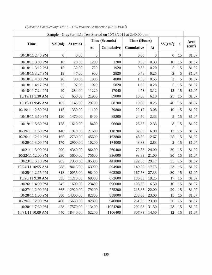
195
Hydraulic Conductivity: Test 1 – 11% Proctor Compaction (67.85 kJ/m3)
Sample - GrayPermL1: Test Started on 10/18/2011 at 2:40:00 p.m.
Time Vol(ml) Δt (min) Time (Seconds) Time (Hours)
ΔV(cm3) i
Area
(cm2) Δt Cumulative Cumulative Δt
10/18/11 2:40 PM 0 0.00 0 0 0.00 0 0 15 81.07
10/18/11 3:00 PM 10 20.00 1200 1200 0.33 0.33 10 15 81.07
10/18/11 3:12 PM 15 32.00 720 1920 0.53 0.20 5 15 81.07
10/18/11 3:27 PM 18 47.00 900 2820 0.78 0.25 3 5 81.07
10/18/11 4:00 PM 20 80.00 1980 4800 1.33 0.55 2 5 81.07
10/18/11 4:17 PM 25 97.00 1020 5820 1.62 0.28 5 15 81.07
10/18/11 7:24 PM 40 284.00 11220 17040 4.73 3.12 15 15 81.07
10/19/11 1:30 AM 65 650.00 21960 39000 10.83 6.10 25 15 81.07
10/19/11 9:45 AM 105 1145.00 29700 68700 19.08 8.25 40 15 81.07
10/19/11 12:50 PM 115 1330.00 11100 79800 22.17 3.08 10 15 81.07
10/19/11 3:10 PM 120 1470.00 8400 88200 24.50 2.33 5 15 81.07
10/19/11 5:30 PM 128 1610.00 8400 96600 26.83 2.33 8 15 81.07
10/19/11 11:30 PM 140 1970.00 21600 118200 32.83 6.00 12 15 81.07
10/20/11 12:10 PM 165 2730.00 45600 163800 45.50 12.67 25 15 81.07
10/20/11 3:00 PM 170 2900.00 10200 174000 48.33 2.83 5 15 81.07
10/21/11 3:00 PM 200 4340.00 86400 260400 72.33 24.00 30 15 81.07
10/22/11 12:00 PM 230 5600.00 75600 336000 93.33 21.00 30 15 81.07
10/23/11 5:10 PM 265 7350.00 105000 441000 122.50 29.17 35 15 81.07
10/24/11 10:55 AM 288 8415.00 63900 504900 140.25 17.75 23 15 81.07
10/25/11 2:15 PM 318 10055.00 98400 603300 167.58 27.33 30 15 81.07
10/26/11 9:30 AM 335 11210.00 69300 672600 186.83 19.25 17 15 81.07
10/26/11 4:00 PM 345 11600.00 23400 696000 193.33 6.50 10 15 81.07
10/27/11 2:00 PM 365 12920.00 79200 775200 215.33 22.00 20 15 81.07
10/28/11 1:00 PM 380 14300.00 82800 858000 238.33 23.00 15 15 81.07
10/29/11 12:00 PM 400 15680.00 82800 940800 261.33 23.00 20 15 81.07
10/30/11 7:30 PM 428 17570.00 113400 1054200 292.83 31.50 28 15 81.07
10/31/11 10:00 AM 440 18440.00 52200 1106400 307.33 14.50 12 15 81.07

196
qin
(cm3/sec)
qout
(cm3/sec)
k (cm/sec) k
(m/sec)
Height of
Water
(cm)
Height of
Water
(in)
Time
Step NPV
Qin (mL)
Cumulative
0 0 0.00 0.00 30.32 11.938 1 0.00 0
2.03E-02 8.33E-03 6.85E-06 6.85E-08 30.16 11.875 2 0.03 10
0.00E+00 6.94E-03 5.71E-06 5.71E-08 30.00 11.813 3 0.04 15
2.70E-02 3.33E-03 8.22E-06 8.22E-08 30.00 11.813 4 0.05 18
0.00E+00 1.01E-03 2.49E-06 2.49E-08 29.85 11.750 5 0.05 20
0.00E+00 4.90E-03 4.03E-06 4.03E-08 29.85 11.750 6 0.06 25
4.34E-03 1.34E-03 1.10E-06 1.10E-08 29.85 11.750 7 0.10 40
1.11E-03 1.14E-03 9.36E-07 9.36E-09 29.53 11.625 8 0.16 65
8.19E-04 1.35E-03 1.11E-06 1.11E-08 29.37 11.563 9 0.26 105
0.00E+00 9.01E-04 7.41E-07 7.41E-09 29.21 11.500 10 0.29 115
0.00E+00 5.95E-04 4.89E-07 4.89E-09 29.21 11.500 11 0.30 120
5.79E-03 9.52E-04 7.83E-07 7.83E-09 29.21 11.500 12 0.32 128
1.13E-03 5.56E-04 4.57E-07 4.57E-09 28.89 11.375 13 0.35 140
0.00E+00 5.48E-04 4.51E-07 4.51E-09 28.73 11.313 14 0.41 165
-2.38E-03 4.90E-04 4.03E-07 4.03E-09 28.73 11.313 15 0.43 170
8.44E-04 3.47E-04 2.86E-07 2.86E-09 28.89 11.375 16 0.50 200
6.43E-04 3.97E-04 3.26E-07 3.26E-09 28.42 11.188 17 0.58 230
2.32E-04 3.33E-04 2.74E-07 2.74E-09 28.10 11.063 18 0.66 265
7.61E-04 3.60E-04 2.96E-07 2.96E-09 27.94 11.000 19 0.72 288
2.47E-04 3.05E-04 2.51E-07 2.51E-09 27.62 10.875 20 0.80 318
3.51E-04 2.45E-04 2.02E-07 2.02E-09 27.46 10.813 21 0.84 335
1.04E-03 4.27E-04 3.51E-07 3.51E-09 27.31 10.750 22 0.86 345
3.07E-04 2.53E-04 2.08E-07 2.08E-09 27.15 10.688 23 0.91 365
2.94E-04 1.81E-04 1.49E-07 1.49E-09 26.99 10.625 24 0.95 380
2.94E-04 2.42E-04 1.99E-07 1.99E-09 26.83 10.563 25 1.00 400
4.29E-04 2.47E-04 2.03E-07 2.03E-09 26.67 10.500 26 1.07 428
7.73E-02 2.30E-04 1.89E-07 1.89E-09 26.35 10.375 27 1.10 440

197
Hydraulic Conductivity: Test 2 – 11% Proctor Compaction (67.85 kJ/m3)
Sample - GrayPermL2: Test Started on 10/18/2011 at 2:40:00 p.m.
Time Vol(ml) Δt (min) Time (Seconds) Time (Hours) ΔV
(cm3)
i Area
(cm2) Δt Cumulative Cumulative Δt
10/18/11 2:40 PM 0 0.00 0 0 0.00 0 0 15 81.07
10/18/11 3:00 PM 145 20.00 1200 1200 0.33 0.33 145 15 81.07
10/18/11 3:12 PM 190 32.00 720 1920 0.53 0.20 45 15 81.07
10/18/11 3:27 PM 238 47.00 900 2820 0.78 0.25 48 5 81.07
10/18/11 4:00 PM 338 80.00 1980 4800 1.33 0.55 100 5 81.07
10/18/11 4:17 PM 380 97.00 1020 5820 1.62 0.28 42 15 81.07
10/18/11 7:24 PM 825 284.00 11220 17040 4.73 3.12 445 15 81.07
10/19/11 1:30 AM 1555 650.00 21960 39000 10.83 6.10 730 15 81.07
10/19/11 9:45 AM 1988 1145.00 29700 68700 19.08 8.25 433 15 81.07
10/19/11 12:50 PM 2033 1330.00 11100 79800 22.17 3.08 45 15 81.07
10/19/11 3:10 PM 2056 1470.00 8400 88200 24.50 2.33 23 15 81.07
10/19/11 5:30 PM 2078 1610.00 8400 96600 26.83 2.33 22 15 81.07
10/19/11 11:30 PM 2128 1970.00 21600 118200 32.83 6.00 50 15 81.07
10/20/11 12:10 PM 2248 2730.00 45600 163800 45.50 12.67 120 15 81.07
10/20/11 3:00 PM 2270 2900.00 10200 174000 48.33 2.83 22 15 81.07
10/21/11 3:00 PM 2376 4340.00 86400 260400 72.33 24.00 106 15 81.07
10/22/11 12:00 PM 2458 5600.00 75600 336000 93.33 21.00 82 15 81.07
10/23/11 5:10 PM 2568 7350.00 105000 441000 122.50 29.17 110 15 81.07
10/24/11 10:55 AM 2653 8415.00 63900 504900 140.25 17.75 85 15 81.07
10/25/11 2:15 PM 2758 10055.00 98400 603300 167.58 27.33 105 15 81.07
10/26/11 9:30 AM 2803 11210.00 69300 672600 186.83 19.25 45 15 81.07
10/26/11 4:00 PM 2818 11600.00 23400 696000 193.33 6.50 15 15 81.07
10/27/11 2:00 PM 2843 12920.00 79200 775200 215.33 22.00 25 15 81.07
10/28/11 1:00 PM 2868 14300.00 82800 858000 238.33 23.00 25 15 81.07
10/29/11 12:00 PM 2890 15680.00 82800 940800 261.33 23.00 22 15 81.07
10/30/11 7:30 PM 2918 17570.00 113400 1054200 292.83 31.50 28 15 81.07
10/31/11 10:00 AM 2936 18440.00 52200 1106400 307.33 14.50 18 15 81.07

198
qin
(cm3/sec)
qout
(cm3/sec)
k
(cm/sec)
k
(m/sec)
Height of
Water
(cm)
Height of
Water
(in)
Time
Step NPV
Qin (mL)
Cumulative
0 0 0.00 0.00 30.16 11.875 1 0.00 0
4.05E-02 1.21E-01 9.94E-05 9.94E-07 29.21 11.500 2 0.38 145
6.76E-02 6.25E-02 5.14E-05 5.14E-07 28.89 11.375 3 0.49 190
1.35E-01 5.33E-02 1.32E-04 1.32E-06 28.58 11.250 4 0.62 238
1.23E-02 5.05E-02 1.25E-04 1.25E-06 27.78 10.938 5 0.88 338
4.29E-01 4.12E-02 3.39E-05 3.39E-07 27.62 10.875 6 0.99 380
6.72E-02 3.97E-02 3.26E-05 3.26E-07 24.77 9.750 7 2.14 825
3.99E-02 3.32E-02 2.73E-05 2.73E-07 19.84 7.813 8 4.03 1555
1.64E-03 1.46E-02 1.20E-05 1.20E-07 14.13 5.563 9 5.15 1988
2.19E-03 4.05E-03 3.33E-06 3.33E-08 13.81 5.438 10 5.27 2033
0.00E+00 2.74E-03 2.25E-06 2.25E-08 13.65 5.375 11 5.33 2056
8.69E-03 2.62E-03 2.15E-06 2.15E-08 13.65 5.375 12 5.39 2078
-1.24E-02 2.31E-03 1.90E-06 1.90E-08 13.18 5.188 13 5.52 2128
9.07E-03 2.63E-03 2.16E-06 2.16E-08 14.92 5.875 14 5.83 2248
1.19E-02 2.16E-03 1.77E-06 1.77E-08 12.22 4.813 15 5.88 2270
8.44E-04 1.23E-03 1.01E-06 1.01E-08 11.43 4.500 16 6.16 2376
1.61E-03 1.08E-03 8.92E-07 8.92E-09 10.95 4.313 17 6.37 2458
9.27E-04 1.05E-03 8.61E-07 8.61E-09 10.16 4.000 18 6.66 2568
1.52E-03 1.33E-03 1.09E-06 1.09E-08 9.53 3.750 19 6.88 2653
4.94E-04 1.07E-03 8.77E-07 8.77E-09 8.89 3.500 20 7.15 2758
3.51E-04 6.49E-04 5.34E-07 5.34E-09 8.57 3.375 21 7.27 2803
0.00E+00 6.41E-04 5.27E-07 5.27E-09 8.41 3.313 22 7.30 2818
6.14E-04 3.16E-04 2.60E-07 2.60E-09 8.41 3.313 23 7.37 2843
2.94E-04 3.02E-04 2.48E-07 2.48E-09 8.10 3.188 24 7.43 2868
5.87E-04 2.66E-04 2.18E-07 2.18E-09 7.94 3.125 25 7.49 2890
0.00E+00 2.47E-04 2.03E-07 2.03E-09 7.62 3.000 26 7.56 2918
2.24E-02 3.45E-04 2.84E-07 2.84E-09 7.62 3.000 27 7.61 2936

199
Hydraulic Conductivity: Test 3 – 11% Proctor Compaction (67.85 kJ/m3)
Sample - GrayPermL3: Test Started on 10/18/2011 at 2:40:00 p.m.
Time Vol(ml) Δt (min) Time (Seconds) Time (Hours) ΔV
(cm3)
i Area
(cm2) Δt Cumulative Cumulative Δt
10/18/11 2:40 PM 0 0.00 0 0 0.00 0 0 15 81.07
10/18/11 3:00 PM 122 20.00 1200 1200 0.33 0.33 122 15 81.07
10/18/11 3:12 PM 137 32.00 720 1920 0.53 0.20 15 15 81.07
10/18/11 3:27 PM 152 47.00 900 2820 0.78 0.25 15 5 81.07
10/18/11 4:00 PM 182 80.00 1980 4800 1.33 0.55 30 5 81.07
10/18/11 4:17 PM 200 97.00 1020 5820 1.62 0.28 18 15 81.07
10/18/11 7:24 PM 430 284.00 11220 17040 4.73 3.12 230 15 81.07
10/19/11 1:30 AM 890 650.00 21960 39000 10.83 6.10 460 15 81.07
10/19/11 9:45 AM 1678 1145.00 29700 68700 19.08 8.25 788 15 81.07
10/19/11 12:50 PM 1708 1330.00 11100 79800 22.17 3.08 30 15 81.07
10/19/11 3:10 PM 1728 1470.00 8400 88200 24.50 2.33 20 15 81.07
10/19/11 5:30 PM 1756 1610.00 8400 96600 26.83 2.33 28 15 81.07
10/19/11 11:30 PM 1818 1970.00 21600 118200 32.83 6.00 62 15 81.07
10/20/11 12:10 PM 2153 2730.00 45600 163800 45.50 12.67 335 15 81.07
10/20/11 3:00 PM 2228 2900.00 10200 174000 48.33 2.83 75 15 81.07
10/21/11 3:00 PM 2396 4340.00 86400 260400 72.33 24.00 168 15 81.07
10/22/11 12:00 PM 2548 5600.00 75600 336000 93.33 21.00 152 15 81.07
10/23/11 5:10 PM 2788 7350.00 105000 441000 122.50 29.17 240 15 81.07
10/24/11 10:55 AM 2953 8415.00 63900 504900 140.25 17.75 165 15 81.07
10/25/11 2:15 PM 3178 10055.00 98400 603300 167.58 27.33 225 15 81.07
10/26/11 9:30 AM 3298 11210.00 69300 672600 186.83 19.25 120 15 81.07
10/26/11 4:00 PM 3316 11600.00 23400 696000 193.33 6.50 18 15 81.07
10/27/11 2:00 PM 3348 12920.00 79200 775200 215.33 22.00 32 15 81.07
10/28/11 1:00 PM 3386 14300.00 82800 858000 238.33 23.00 38 15 81.07
10/29/11 12:00 PM 3416 15680.00 82800 940800 261.33 23.00 30 15 81.07
10/30/11 7:30 PM 3471 17570.00 113400 1054200 292.83 31.50 55 15 81.07
10/31/11 10:00 AM 3496 18440.00 52200 1106400 307.33 14.50 25 15 81.07

200
qin
(cm3/sec)
qout
(cm3/sec)
k
(cm/sec) k (m/sec)
Height of
Water
(cm)
Height of
Water
(in)
Time
Step NPV
Qin (mL)
Cumulative
0 0 0.00 0.00 26.51 10.438 1 0.00 0
2.03E-02 1.02E-01 8.36E-05 8.36E-07 26.35 10.375 2 0.32 122
0.00E+00 2.08E-02 1.71E-05 1.71E-07 26.19 10.313 3 0.35 137
5.40E-02 1.67E-02 4.11E-05 4.11E-07 26.19 10.313 4 0.39 152
1.23E-02 1.52E-02 3.74E-05 3.74E-07 25.88 10.188 5 0.47 182
1.91E-01 1.76E-02 1.45E-05 1.45E-07 25.72 10.125 6 0.52 200
4.34E-02 2.05E-02 1.69E-05 1.69E-07 24.45 9.625 7 1.11 430
3.21E-02 2.09E-02 1.72E-05 1.72E-07 21.27 8.375 8 2.30 890
1.64E-03 2.65E-02 2.18E-05 2.18E-07 16.67 6.563 9 4.34 1678
2.19E-03 2.70E-03 2.22E-06 2.22E-08 16.35 6.438 10 4.42 1708
2.90E-03 2.38E-03 1.96E-06 1.96E-08 16.19 6.375 11 4.47 1728
8.69E-03 3.33E-03 2.74E-06 2.74E-08 16.03 6.313 12 4.54 1756
1.46E-02 2.87E-03 2.36E-06 2.36E-08 15.56 6.125 13 4.70 1818
1.60E-03 7.35E-03 6.04E-06 6.04E-08 13.49 5.313 14 5.57 2153
1.67E-02 7.35E-03 6.05E-06 6.05E-08 13.02 5.125 15 5.76 2228
1.69E-03 1.94E-03 1.60E-06 1.60E-08 11.91 4.688 16 6.19 2396
2.90E-03 2.01E-03 1.65E-06 1.65E-08 10.95 4.313 17 6.59 2548
1.85E-03 2.29E-03 1.88E-06 1.88E-08 9.53 3.750 18 7.21 2788
3.81E-03 2.58E-03 2.12E-06 2.12E-08 8.26 3.250 19 7.63 2953
9.89E-04 2.29E-03 1.88E-06 1.88E-08 6.67 2.625 20 8.21 3178
7.02E-04 1.73E-03 1.42E-06 1.42E-08 6.03 2.375 21 8.53 3298
1.04E-03 7.69E-04 6.33E-07 6.33E-09 5.72 2.250 22 8.57 3316
9.21E-04 4.04E-04 3.32E-07 3.32E-09 5.56 2.188 23 8.65 3348
2.94E-04 4.59E-04 3.77E-07 3.77E-09 5.08 2.000 24 8.75 3386
5.87E-04 3.62E-04 2.98E-07 2.98E-09 4.92 1.938 25 8.83 3416
2.14E-04 4.85E-04 3.99E-07 3.99E-09 4.60 1.813 26 8.97 3471
1.30E-02 4.79E-04 3.94E-07 3.94E-09 4.45 1.750 27 9.04 3496

201
Appendix II – Compaction Data
Standard Proctor Compaction (592.5 kJ/m3)
Compaction Energy kJ/m3 (ft-lb/ft
3) 592.5 (12375)
Test Number 1 2 3 4
Assumed moisture content (%) 14.00 11.00 8.00 6.00
Mold Weight (g), Mmd 2044.62 2044.62 2044.62 2044.62
Specimen+Mold Weight (g), Mt 3846.50 4024.33 3998.61 3434.61
Volume of Mold (cm3), V 940.00 940.00 940.00 940.00
Specific Gravity of Soil, Gs 2.69 2.69 2.69 2.69
Unit Weight of Water @ 20oC(KN/m
3), γw 9.79 9.79 9.79 9.79
Unit Weight of Water @ 20oC(lb/ft
3), γw 62.34 62.34 62.34 62.34
Moist Unit Weight of Compacted Specimen(g/cm3), γm 1.92 2.11 2.08 1.48
Dry Unit Weight of Compacted Specimen(g/cm3), γd 1.70 1.89 1.89 1.42
Dry Unit Weight of Compacted Specimen(KN/m3), γd 16.65 18.51 18.54 13.92
Dry Unit Weight of Compacted Specimen(lb/ft3), γd 106.04 117.87 118.04 88.67
Dry Unit Weight at S=1.0 (KN/m3),γd 19.57 20.09 20.78 23.71
Dry Unit Weight at S=0.9 (KN/m3),γd 19.03 19.58 20.30 23.45
Dry Unit Weight at S=1.0 (lb/ft3), γd 124.61 127.96 132.32 150.98
Dry Unit Weight at S=0.9 (lb/ft3), γd 121.15 124.68 129.29 149.32
Void Ratio, e=((Gs*γw)/γd)-1 0.58 0.42 0.42 0.89
Degree of Saturation (%), S=Gs*w/e 0.59 0.73 0.64 0.12
Saturated Water Content, wsat(%) 21.62 15.71 15.64 33.14
Moisture Content:
Test Number 1 2 3 4
Assumed moisture content (%) 14.00 11.00 8.00 6.00
Container Mass (g), Mc 30.03 17.27 30.55 18.84
Container+Moist Specimen Mass (g), Mcms 90.43 70.70 77.78 41.60
Intial Container+Oven Dry Specimen Mass (g), Mcds 83.55 65.17 73.51 40.70
Mass of Water(g), Mw= Mcms-Mcds 6.88 5.53 4.27 0.90
Mass of Solids (g), Ms= Mcds-Mc 53.52 47.90 42.96 21.86
Water Content, w=(Mw/Ms)x100(%) 12.86 11.54 9.94 4.12

202
34% Proctor Compaction Energy: (203.6 kJ/m3)
Compaction Energy kJ/m3 (ft-lb/ft
3) 203.6 (4252)
Test Number 1 2 3 4 5 6 7
Assumed moisture content (%) 3.00 6.00 9.00 14.00 12.00 15.00 12.00
Mold Weight (g), Mmd 1985.84 1985.84 1985.84 1985.84 1985.84 1985.84 1985.84
Specimen Weight (g) 1660.06 1703.00 1757.33 1945.49 1939.41 1974.56 1625.31
Specimen+Mold Weight (g), Mt 3645.90 3688.84 3743.17 3931.33 3925.25 3960.40 3611.15
Volume of Mold (cm3),
V 940.00 940.00 940.00 940.00 940.00 940.00 940.00
Specific Gravity of Soil, Gs 2.69 2.69 2.69 2.69 2.69 2.69 2.69
Unit Weight of Water @ 20oC (KN/m
3), γw 9.79 9.79 9.79 9.79 9.79 9.79 9.79
Unit Weight of Water @ 20oC (lb/ft
3), γw 62.34 62.34 62.34 62.34 62.34 62.34 62.34
Moist Unit Weight of Compacted Specimen
(g/cm3), γm 1.77 1.81 1.87 2.07 2.06 2.10 1.73
Dry Unit Weight of Compacted Specimen
(g/cm3), γd 1.64 1.65 1.68 1.83 1.83 1.82 1.47
Dry Unit Weight of Compacted Specimen
(KN/m3), γd 16.11 16.21 16.48 17.98 17.94 17.80 14.37
Dry Unit Weight of Compacted Specimen
(lb/ft3), γd 102.61 103.23 104.96 114.49 114.26 113.32 91.50
Dry Unit Weight at S=1.0 (KN/m3),γd 21.94 20.95 20.24 19.57 19.62 18.51 17.75
Dry Unit Weight at S=0.9 (KN/m3),γd 21.54 20.48 19.73 19.03 19.08 17.91 17.13
Dry Unit Weight at S=1.0 (lb/ft3), γd 139.72 133.38 128.87 124.61 124.92 117.84 113.05
Dry Unit Weight at S=0.9 (lb/ft3), γd 137.17 130.41 125.63 121.15 121.48 114.07 109.10
Void Ratio, e=((Gs*γw)/γd)-1 0.63 0.62 0.60 0.46 0.47 0.48 0.83
Degree of Saturation (%), S=Gs*w/e 0.32 0.41 0.50 0.74 0.73 0.88 0.58
Saturated Water Content, wsat (%) 23.58 23.22 22.22 17.28 17.39 17.84 30.96

203
Moisture Content:
Test Number 1 2 3 4 5 6 7
Assumed moisture content (%) 3.00 6.00 9.00 14.00 12.00 14.00 12.00
Container Mass (g), Mc 16.74 30.45 30.69 18.73 17.40 22.00 30.11
Container+Moist Specimen Mass (g), Mcms 68.55 128.84 128.77 78.87 85.68 99.55 131.87
Intial Container+Oven Dry Specimen Mass (g), Mcds 64.96 120.25 118.89 72.02 77.97 89.01 116.37
Mass of Water (g), Mw= Mcms-Mcds 3.59 8.59 9.88 6.85 7.71 10.54 15.50
Mass of Solids (g), Ms= Mcds-Mc 48.22 89.80 88.20 53.29 60.57 67.01 86.26
Water Content, (%) W= (Mw/Ms)x100 7.45 9.57 11.20 12.85 12.73 15.73 17.97

204
11% Proctor Compaction Energy: (67.85 kJ/m3)
Compaction Energy kJ/m3 (ft-lb/ft
3) 67.85 (1417)
Test Number 1 2 3 4 5 6 7
Assumed moisture content (%) 3.00 9.00 8.00 12.00 6.00 12.00 17.00
Mold Weight (g), Mmd 1985.84 1985.84 1985.84 1985.84 1985.84 1985.84 1985.84
Specimen Weight (g) 1539.63 1871.31 1626.85 1571.22 1613.3 1972.17 1864
Specimen+Mold Weight (g), Mt 3525.47 3857.15 3612.69 3557.06 3599.14 3958.01 3849.84
Volume of Mold (cm3),
V 940.00 940.00 940.00 940.00 940.00 940.00 940.00
Specific Gravity of Soil, Gs 2.69 2.69 2.69 2.69 2.69 2.69 2.69
Unit Weight of Water @ 20oC (KN/m
3), γw 9.79 9.79 9.79 9.79 9.79 9.79 9.79
Unit Weight of Water @ 20oC (lb/ft
3), γw 62.34 62.34 62.34 62.34 62.34 62.34 62.34
Moist Unit Weight of Compacted Specimen (g/cm3),
γm 1.64 1.99 1.73 1.67 1.72 2.10 1.98
Dry Unit Weight of Compacted Specimen (g/cm3), γd 1.57 1.72 1.55 1.52 1.54 1.79 1.69
Dry Unit Weight of Compacted Specimen (KN/m3),
γd 15.39 16.90 15.20 14.93 15.07 17.60 16.55
Dry Unit Weight of Compacted Specimen (lb/ft3), γd 97.98 107.64 96.82 95.05 95.97 112.05 105.40
Dry Unit Weight at S=1.0 (KN/m3),γd 23.57 18.60 20.07 20.85 20.05 18.11 17.92
Dry Unit Weight at S=0.9 (KN/m3),γd 23.30 18.01 19.55 20.38 19.53 17.50 17.31
Dry Unit Weight at S=1.0 (lb/ft3), γd 150.09 118.43 127.81 132.76 127.68 115.31 114.12
Dry Unit Weight at S=0.9 (lb/ft3), γd 148.36 114.68 124.52 129.75 124.38 111.44 110.20
Void Ratio, e=((Gs*γw)/γd)-1 0.71 0.56 0.73 0.76 0.75 0.50 0.59
Degree of Saturation (%), S=Gs*w/e 0.16 0.75 0.43 0.34 0.42 0.92 0.79
Saturated Water Content, wsat (%) 26.45 20.74 27.22 28.41 27.79 18.46 21.97

205
Moisture Content:
Test Number 1 2 3 4 5 6 7
Assumed moisture content (%) 3.00 9.00 8.00 12.00 6.00 12.00 17.00
Container Mass (g), Mc 17.42 18.86 18.84 17.42 18.77 30.59 30
Container+Moist Specimen Mass (g), Mcms 71.98 84.78 100.32 102.02 83.17 155.85 85.92
Intial Container+Oven Dry Specimen Mass (g), Mcds 69.70 75.95 91.85 94.48 76.45 137.75 77.61
Mass of Water (g), Mw= Mcms-Mcds 2.28 8.83 8.47 7.54 6.72 18.10 8.31
Mass of Solids (g), Ms= Mcds-Mc 52.28 57.09 73.01 77.06 57.68 107.16 47.61
Water Content, (%) W= (Mw/Ms)x100 4.36 15.47 11.60 9.78 11.65 16.89 17.45

206
Appendix III – Grain Size Distribution Testing Data
Post-Permeability Grain Size Distribution Data
Standard Proctor Effort – Sieve analysis data for layer 1 and layer 2
Sieve Analysis
Sieve No. Particle dia.
(mm) Empty Pan Wt. Retained+pan Wt. Retained % Retained Cumulative % Percent Finer
Layer 1 Layer 2 Layer 1 Layer 2 Layer 1 Layer 2 Layer 1 Layer 2 Layer 1 Layer 2 Layer 1 Layer 2
2'' 50.80 775.71 775.71 775.71 775.71 0.00 0.00 0.00 0.00 0.00 0.00 100.00 100.00
No. 4 4.76 557.13 557.13 557.13 557.13 0.00 0.00 0.00 0.00 0.00 0.00 100.00 100.00
No. 10 2.00 469.11 469.11 680.54 768.01 211.43 298.90 39.74 47.31 39.74 47.31 60.26 52.69
No.30 0.60 396.30 396.30 584.04 579.53 187.74 183.23 35.29 29.00 75.03 76.31 24.97 23.69
No. 50 0.30 370.07 370.07 418.28 426.73 48.21 56.66 9.06 8.97 84.10 85.28 15.90 14.72
No.60 0.25 317.98 317.98 327.81 328.64 9.83 10.66 1.85 1.69 85.94 86.96 14.06 13.04
No.200 0.08 293.88 293.88 332.48 335.74 38.60 41.86 7.26 6.63 93.20 93.59 6.80 6.41
Pan 369.66 369.66 405.53 406.74 35.87 37.08 6.74 5.87 99.94 99.46 0.06 0.54
Total 531.68 628.39 99.94 99.46
Layer 1 Layer 2 Layer 3
Mass of Sample 531.98 631.81 489.78
Mass Loss(%) 0.06 0.54 0.00

207
Standard Proctor Effort – Sieve analysis data for layer 3
Sieve Analysis
Sieve No. Particle dia.
(mm)
Empty
Pan
Wt.
Retained+pan Wt. Retained % Retained Cumulative %
Percent
Finer
Layer 3 Layer 3 Layer 3 Layer 3 Layer 3 Layer 3
2'' 50.80 775.71 775.71 0.00 0.00 0.00 100.00
No. 4 4.76 557.13 557.13 0.00 0.00 0.00 100.00
No. 10 2.00 469.11 687.10 217.99 44.51 44.51 55.49
No.30 0.60 396.30 553.63 157.33 32.12 76.63 23.37
No. 50 0.30 370.07 411.06 40.99 8.37 85.00 15.00
No.60 0.25 317.98 326.60 8.62 1.76 86.76 13.24
No.200 0.08 293.88 326.84 32.96 6.73 93.49 6.51
Pan 369.66 401.56 31.90 6.51 100.00 0.00
Total 489.79 100.00

208
34% Proctor Compaction Effort
Sieve Analysis
Sieve
No.
Particle
dia.
(mm)
Empty Pan Wt Retained+pan Wt Retained % Retained Cumulative % Percent Finer
Layer
1
Layer
2
Layer
3
Layer
1
Layer
2
Layer
3
Layer
1
Layer
2
Layer
3
Layer
1
Layer
2
Layer
3
Layer
1
Layer
2
Layer
3
Layer
1
Layer
2
Layer
3
2'' 50.8 775.88 775.88 775.88 775.88 775.88 775.88 0 0 0 0.00 0.00 0.00 0.00 0.00 0.00 100.00 100 100.00
No. 4 4.76 557.33 557.33 557.33 557.33 557.33 557.33 0 0 0 0.00 0.00 0.00 0.00 0.00 0.00 100.00 100.00 100.00
No. 10 2.00 479.24 479.31 479.23 664.52 733.52 719.19 185.28 254.21 239.96 41.51 42.48 47.26 41.51 42.48 47.26 58.49 57.52 52.74
No.30 0.39 482.31 482.21 482.32 617.17 666.66 640.22 134.86 184.45 157.9 30.21 30.82 31.10 71.73 73.30 78.35 28.27 26.70 21.65
No. 50 0.30 370.94 371.14 371 415.61 427.04 410.72 44.67 55.9 39.72 10.01 9.34 7.82 81.73 82.64 86.18 18.27 17.36 13.82
No.60 0.25 367.1 367.26 367.26 378.21 381.11 376.06 11.11 13.85 8.8 2.49 2.31 1.73 84.22 84.95 87.91 15.78 15.05 12.09
No.200 0.08 338.1 338.09 338.09 374.84 386.07 372.26 36.74 47.98 34.17 8.23 8.02 6.73 92.45 92.97 94.64 7.55 7.03 5.36
Pan
370.93 370.96 370.91 404.34 411.82 397.85 33.41 40.86 26.94 7.49 6.83 5.31 99.94 99.80 99.94 0.06 0.20 0.06
Total 446.07 597.25 507.49 99.94 99.80 99.94
Layer
1
Layer
2
Layer
3
Mass of Sample 446.34 598.45 507.78
Mass Loss(%) 0.06 0.20 0.06

209
11% Proctor Compaction Effort – Test 1
Sieve Analysis
Sieve
No.
Particle
dia.
(mm)
Empty Pan Wt Retained+pan Wt Retained % Retained Cumulative % Percent Finer
Layer
1
Layer
2
Layer
3
Layer
1
Layer
2
Layer
3
Layer
1
Layer
2
Layer
3
Layer
1
Layer
2
Layer
3
Layer
1
Layer
2
Layer
3
Layer
1
Layer
2
Layer
3
2'' 50.8 775.73 775.73 775.73 775.73 775.73 775.73 0 0 0 0.00 0.00 0.00 0.00 0.00 0.00 100.00 100 100.00
No. 4 4.76 557.2 557.2 557.2 557.2 557.2 557.2 0 0 0 0.00 0.00 0.00 0.00 0.00 0.00 100.00 100.00 100.00
No. 10 2.00 479.34 479.26 479.18 597.1 656.21 673.85 117.76 176.95 194.67 34.73 39.86 38.95 34.73 39.86 38.95 65.27 60.14 61.05
No.30 0.39 482.35 482.37 482.02 598.08 619.30 643.07 115.73 136.93 161.05 34.13 30.84 32.22 68.86 70.70 71.17 31.14 29.30 28.83
No. 50 0.30 370.97 370.99 370.71 407.53 417.06 423.44 36.56 46.07 52.73 10.78 10.38 10.55 79.64 81.07 81.72 20.36 18.93 18.28
No.60 0.25 367.13 367.13 366.83 375.93 378.62 379.78 8.8 11.49 12.95 2.60 2.59 2.59 82.24 83.66 84.31 17.76 16.34 15.69
No.200 0.08 337.99 338.01 337.78 369.86 375.70 379 31.87 37.69 41.22 9.40 8.49 8.25 91.64 92.15 92.56 8.36 7.85 7.44
Pan 370.97 370.94 370.72 399.2 404.12 408.19 28.23 33.18 37.47 8.33 7.47 7.50 99.96 99.62 100.06 0.04 0.38 -0.06
Total 338.95 442.31 500.09 99.96 99.62 100.06
Layer
1
Layer
2
Layer
3
Mass of Sample 339.07 443.98 499.80
Mass Loss(%) 0.04 0.38 -0.06

210
11% Proctor Compaction Effort – Test 2
Sieve Analysis
Sieve
No.
Particle
dia.
(mm)
Empty Pan Wt Retained+pan Wt Retained % Retained Cumulative % Percent Finer
Layer
1
Layer
2
Layer
3
Layer
1
Layer
2
Layer
3
Layer
1
Layer
2
Layer
3
Layer
1
Layer
2
Layer
3
Layer
1
Layer
2
Layer
3
Layer
1
Layer
2
Layer
3
2'' 50.8 775.73 775.73 775.88 775.73 775.73 775.88 0 0 0 0.00 0.00 0.00 0.00 0.00 0.00 100.00 100 100.00
No. 4 4.76 557.2 557.2 557.33 557.2 557.2 557.33 0 0 0 0.00 0.00 0.00 0.00 0.00 0.00 100.00 100.00 100.00
No. 10 2.00 478.99 478.99 479.08 608.67 657.90 673.45 129.68 178.91 194.37 35.65 34.63 38.16 35.65 34.63 38.16 64.35 65.37 61.84
No.30 0.39 482.15 482.02 482.13 607.49 662.23 646.79 125.34 180.21 164.66 34.46 34.88 32.32 70.11 69.50 70.48 29.89 30.50 29.52
No. 50 0.30 370.7 370.78 370.8 409.15 426.85 422.96 38.45 56.07 52.16 10.57 10.85 10.24 80.68 80.36 80.72 19.32 19.64 19.28
No.60 0.25 366.9 366.95 366.96 375.5 380.20 380.11 8.6 13.25 13.15 2.36 2.56 2.58 83.04 82.92 83.30 16.96 17.08 16.70
No.200 0.08 337.82 337.87 337.8 368.23 385.64 382.81 30.41 47.77 45.01 8.36 9.25 8.84 91.40 92.17 92.14 8.60 7.83 7.86
Pan 370.75 370.77 370.75 401.03 411.13 410.62 30.28 40.36 39.87 8.32 7.81 7.83 99.73 99.98 99.96 0.27 0.02 0.04
Total 362.76 516.57 509.22 99.73 99.98 99.96
Layer
1
Layer
2
Layer
3
Mass of Sample 363.75 516.69 509.40
Mass Loss(%) 0.27 0.02 0.04

211
11% Proctor Compaction Effort – Test 3
Sieve Analysis
Sieve
No.
Particle
dia.
(mm)
Empty Pan Wt Retained+pan Wt Retained % Retained Cumulative % Percent Finer
Layer
1
Layer
2
Layer
3
Layer
1
Layer
2
Layer
3
Layer
1
Layer
2
Layer
3
Layer
1
Layer
2
Layer
3
Layer
1
Layer
2
Layer
3
Layer
1
Layer
2
Layer
3
2'' 50.8 775.73 775.73 775.73 775.73 775.73 775.73 0 0 0 0.00 0.00 0.00 0.00 0.00 0.00 100.00 100 100.00
No. 4 4.76 557.2 557.2 557.2 557.2 557.2 557.2 0 0 0 0.00 0.00 0.00 0.00 0.00 0.00 100.00 100.00 100.00
No. 10 2.00 479.19 479.23 479.26 647.7 693.04 677.5 168.51 213.81 198.24 38.73 42.72 47.67 38.73 42.72 47.67 61.27 57.28 52.33
No.30 0.39 481.98 482.17 482.24 626.92 630.48 598.4 144.94 148.31 116.16 33.31 29.63 27.93 72.05 72.35 75.60 27.95 27.65 24.40
No. 50 0.30 370.93 370.96 370.92 414.12 417.82 405.7 43.19 46.86 34.78 9.93 9.36 8.36 81.97 81.72 83.96 18.03 18.28 16.04
No.60 0.25 367.15 367.1 367.03 377.85 378.20 375.67 10.7 11.1 8.64 2.46 2.22 2.08 84.43 83.93 86.04 15.57 16.07 13.96
No.200 0.08 337.94 337.97 338 374.02 379.76 369.35 36.08 41.79 31.35 8.29 8.35 7.54 92.73 92.28 93.58 7.27 7.72 6.42
Pan 370.94 370.89 370.85 402.67 409.82 397.53 31.73 38.93 26.68 7.29 7.78 6.42 100.02 100.06 100.00 -0.02 -0.06 0.00
Total 435.15 500.8 415.85 100.02 100.06 100.00
Layer
1
Layer
2
Layer
3
Mass of Sample 435.06 500.49 415.87
Mass Loss(%) -0.02 -0.06 0.00

212
Pre-Permeability Grain Size Distribution Data
Standard Proctor Compaction Effort – Sieve analysis data for layer 1 and layer 2
Sieve No. Particle dia. (mm) Empty Pan Wt Retained+pan Wt Retained % Retained Cumulative % Percent Finer
Layer 1 Layer 2 Layer 1 Layer 2 Layer 1 Layer 2 Layer 1 Layer2 Layer 1 Layer2 Layer 1 Layer2
0 0 0 0 0 0 100 100
2'' 50.80 637.46 637.46 637.46 637.46 0 0 0 0 0 0 100 100
No. 4 4.760 556.79 556.7 556.79 556.7 0 0 0 0 0 0 100 100
No. 10 2.000 468.86 468.78 631.62 546.41 162.76 77.63 33.53 23.34 33.53 23.34 66.47 76.66
No. 30 0.595 409.52 409.38 561.44 510.89 151.92 101.51 31.3 30.52 64.83 53.86 35.17 46.14
No. 50 0.300 370.72 370.66 451.42 438.17 80.7 67.51 16.63 20.3 81.46 74.16 18.54 25.84
No. 60 0.250 366.81 366.87 385.25 383.01 18.44 16.14 3.8 4.85 85.26 79.01 14.74 20.99
No. 200 0.075 335.07 334.96 383.89 382.17 48.82 47.21 10.06 14.19 95.31 93.2 4.69 6.8
Pan 371.62 371.73 395.12 396.68 23.5 24.95 4.84 7.5 100.15 100.7 -0.15 -0.7
Total 486.14 334.95 100.15 100.7

213
Standard Proctor Compaction Effort - Sieve analysis data for layer 3
Sieve No.
Particle dia.
(mm)
Empty
Pan Wt Retained+pan Wt Retained % Retained
Cumulative
% Percent Finer
Layer 3 Layer 3 Layer 3 Layer 3 Layer 3 Layer 3
0 0 0 100
2'' 50.800 637.46 637.46 0 0 0 100
No. 4 4.760 556.82 556.82 0 0 0 100
No. 10 2.000 468.77 571.22 102.45 36.45 36.45 63.55
No. 30 0.595 409.53 497.56 88.03 31.32 67.76 32.24
No. 50 0.300 370.61 412.06 41.45 14.75 82.51 17.49
No. 60 0.250 366.91 376.47 9.56 3.4 85.91 14.09
No. 200 0.075 334.92 360.41 25.49 9.07 94.98 5.02
Pan 371.69 386.66 14.97 5.33 100.3 -0.3
Total 281.95 100.3
Layer 1 Layer 2 Layer 3
Mass of Sample 485.39 332.61 281.10
Mass Loss(%) -0.15 -0.70 -0.30

214
34% Proctor Compaction Effort – Sieve analysis data for layer 1 and layer 2
Sieve Analysis
Sieve No. Particle dia.
(mm) Empty Pan Wt. Retained+pan Wt. Retained % Retained Cumulative % Percent Finer
Layer 1 Layer 2 Layer 1 Layer 2 Layer 1 Layer 2 Layer 1 Layer 2 Layer 1 Layer 2 Layer 1 Layer 2
2'' 50.80 775.71 775.71 775.71 775.71 0 0 0 0 0 0 100 100
No. 4 4.76 557.43 557.43 557.43 557.43 0 0 0 0 0 0 100 100
No. 10 2.00 479.26 479.26 586.59 575.84 107.33 96.58 36.78 34.00 36.78 34.00 63.22 66.00
No.30 0.60 481.97 481.97 588.68 580.94 106.71 98.97 36.57 34.84 73.34 68.83 26.66 31.17
No. 50 0.30 370.89 370.95 402.09 405.43 31.2 34.48 10.69 12.14 84.04 80.97 15.96 19.03
No.60 0.25 367.06 367.09 374.34 375.76 7.28 8.67 2.49 3.05 86.53 84.02 13.47 15.98
No.200 0.08 338.03 338.03 361.75 364.91 23.72 26.88 8.13 9.46 94.66 93.48 5.34 6.52
Pan 370.9 370.91 388.55 392.06 17.65 21.15 6.05 7.44 100.71 100.93 -0.71 -0.93
Total 293.89 286.73 100.71 100.93
Layer 1 Layer 2 Layer 3
Mass of Sample 291.83 284.09 535.42
Mass Loss(%) -0.71 -0.93 -0.97

215
34% Proctor Compaction Effort - Sieve analysis data for layer 3
Sieve Analysis
Sieve No. Particle
dia. (mm)
Empty
Pan Wt. Retained+pan Wt. Retained % Retained Cumulative %
Percent
Finer
Layer 3 Layer 3 Layer 3 Layer 3 Layer 3 Layer 3
2'' 50.80 775.71 775.71 0 0 0 100
No. 4 4.76 557.43 557.43 0 0 0 100
No. 10 2.00 479.26 657.49 178.23 33.29 33.29 66.71
No.30 0.60 482.09 669.48 187.39 35.00 68.29 31.71
No. 50 0.30 370.94 440.01 69.07 12.90 81.19 18.81
No.60 0.25 367.04 384.94 17.9 3.34 84.53 15.47
No.200 0.08 338.02 387.83 49.81 9.30 93.83 6.17
Pan 370.95 409.14 38.19 7.13 100.97 -0.97
Total 540.59 100.97

216
11% Proctor Compaction Effort – Sieve analysis data for layer 1 and layer 2
Sieve Analysis
Sieve No. Particle
dia. (mm) Empty Pan
Wt.
Retained+pan Wt. Retained % Retained Cumulative % Percent Finer
Layer 1 Layer 2 Layer 1 Layer 2 Layer 1 Layer 2 Layer 1 Layer 2 Layer 1 Layer 2 Layer 1 Layer 2
2'' 50.80 775.63 775.63 775.63 775.63 0 0 0 0 0 0 100 100
No. 4 4.76 557.18 557.18 557.18 557.18 0 0 0 0 0 0 100 100
No. 10 2.00 479.14 479.31 600.53 597.30 121.39 117.99 52.78 50.77 52.78 50.77 47.22 49.23
No.30 0.60 482.20 482.10 550.37 548.19 68.17 66.09 29.64 28.44 82.42 79.21 17.58 20.79
No. 50 0.30 371.00 370.96 386.83 389.37 15.83 18.41 6.88 7.92 89.31 87.13 10.69 12.87
No.60 0.25 367.15 367.15 370.65 371.72 3.50 4.57 1.52 1.97 90.83 89.10 9.17 10.90
No.200 0.08 338.08 337.99 349.37 352.36 11.29 14.37 4.91 6.18 95.74 95.28 4.26 4.72
Pan 369.65 369.6 379.23 380.99 9.58 11.39 4.17 4.90 99.90 100.18 0.10 -0.18
Total 229.76 232.82 99.90 100.18
Layer 1 Layer 2 Layer 3
Mass of Sample 229.98 284.09 535.42
Mass Loss(%) 0.10 -0.93 -0.97

217
11% Proctor Compaction Effort - Sieve analysis data for layer 3
Sieve Analysis
Sieve No. Particle
dia. (mm)
Empty
Pan Wt. Retained+pan Wt. Retained % Retained Cumulative %
Percent
Finer
Layer 3 Layer 3 Layer 3 Layer 3 Layer 3 Layer 3
2'' 50.80 775.63 775.63 0 0 0 100
No. 4 4.76 557.18 557.18 0 0 0 100
No. 10 2.00 479.30 604.95 125.65 46.21 46.21 53.80
No.30 0.60 482.04 572.07 90.03 33.11 79.31 20.69
No. 50 0.30 370.96 394.28 23.32 8.58 87.89 12.11
No.60 0.25 367.07 372.22 5.15 1.89 89.78 10.22
No.200 0.075 338.04 353.88 15.84 5.82 95.61 4.39
Pan 369.67 381.82 12.15 4.47 100.07 -0.07
Total 272.14 100.07

218
As-Received Grain Size Distribution Data: Weathered Sandstone Material
As Received Grain Size Distribution: Weathered Sandstone Material: Test 1, Test 2
Sieve No. Particle dia. (mm) Cumulative % Percent Finer
Test 1 Test 2 Test 1 Test 2
2'' 50.8 0 0 100 100
1" 25.4 7.29 15.04 92.71 84.96
3/4" 19.05 18.27 17.95 81.73 82.05
3/8" 9.5 37.24 30.42 62.76 69.58
No. 4 4.76 55.99 51.7 44.01 48.3
No. 10 2 70.08 68.04 29.92 31.96
No. 40 0.43 84.42 86.76 15.58 13.24
No. 200 0.08 96.13 97.87 3.87 2.13
Pan 99.72 99.77 0.28 0.23
Empty Pan Wt Retained+pan Wt Retained % Retained
Test 1 Test 2 Test 1 Test 2 Test 1 Test 2 Test 1 Test 2
638.02 638.02 638.02 638.02 0 0 0 0
584.26 584.22 620.73 659.4 36.47 75.18 7.29 15.04
587.77 587.8 642.66 602.37 54.89 14.57 10.98 2.91
556.02 555.83 650.86 618.2 94.84 62.37 18.97 12.47
517.72 585.78 611.47 692.18 93.75 106.4 18.75 21.28
472.55 472.51 543 554.2 70.45 81.69 14.09 16.34
375.02 374.98 446.74 468.58 71.72 93.6 14.34 18.72
337.9 337.93 396.45 393.45 58.55 55.52 11.71 11.1
371.84 372.52 389.75 382.03 17.91 9.51 3.58 1.9
Total 498.58 498.84 99.72 99.77

219
As-Received Grain Size Distribution Data: Unweathered Sandstone Overburden
As Received Grain Size Distribution: Unweathered Sandstone Overburden: Test 1, Test 2
Sieve No. Particle dia. (mm) Cumulative % Percent Finer
Test 1 Test 2 Test 1 Test 2
2'' 50.8 0 0 100 100
1" 25.4 0 0 100 100
3/4" 19.05 1.11 7.14 98.89 92.86
3/8" 9.5 14.24 20.4 85.76 79.6
No. 4 4.76 28.83 32.19 71.17 67.81
No. 10 2 45.73 46.62 54.27 53.38
No. 40 0.43 73.73 74.03 26.27 25.97
No. 200 0.08 94.97 95.38 5.03 4.62
Pan 99.88 99.91 0.12 0.09
Empty Pan Wt Retained+pan Wt Retained % Retained
Test 1 Test 2 Test 1 Test 2 Test 1 Test 2 Test 1 Test 2
638.02 638.02 638.02 638.02 0 0 0 0
584.36 584.4 584.36 584.4 0 0 0 0
587.78 587.83 593.31 623.53 5.53 35.7 1.11 7.14
555.97 556.05 621.65 622.34 65.68 66.29 13.14 13.26
517.73 517.68 590.68 576.62 72.95 58.94 14.59 11.79
472.58 472.5 557.05 544.68 84.47 72.18 16.89 14.44
375.07 374.97 515.11 512 140.04 137.03 28.01 27.41
337.93 337.92 444.1 444.66 106.17 106.74 21.23 21.35
371.87 371.81 396.44 394.46 24.57 22.65 4.91 4.53
Total 499.41 499.53 99.88 99.91
Test 1 Test 2
Mass of Sample 500 500
Mass Loss(%) 0.12 0.09