Appendix B-7

Technical Memorandum: Preparation of Wildland Fire Emissions Inventory for 2011

Technical Memorandum

August 15, 2012 STI-910321-5446

To: Venkatesh Rao, U.S. Environmental Protection Agency

From: ShihMing Huang, Yuan Du, Sean M. Raffuse, and Stephen B. Reid

Re: Preparation of Wildland Fire Emissions Inventory for 2011

The U.S. Environmental Protection Agency's (EPA) Emissions Inventory and Analysis

Group (EIAG) compiles the National Emissions Inventory (NEI) and disseminates inventory

data, summaries, model-ready files, and analyses based on the NEI. To support this program

and the analyses conducted by a variety of users, Sonoma Technology, Inc. (STI) has

developed an emissions inventory of wildland fires for the year 2011, as we did for the years

2006 through 2010.

This work was done via Work Assignment (WA) 3-21 under Contract No. EP-D-09-097.

This technical memorandum describes the methods used to develop the 2011 fire emissions

inventory, summarizes the 2011 fire activity and emissions data, and compares the inventories

for the past five years.

Technical Approach

Data Sources

Fire activity data from the following sources were used to develop the 2011 fire

inventory:

· Inputs to SmartFire 2 (SF2)

– HMS data were acquired daily from the National Oceanic and Atmospheric Administration (NOAA) Hazard Mapping System (HMS) via FTP as part of a routine process. Data were acquired in ASCII text format available at http://satepsanone.nesdis.noaa.gov/FIRE/fire.html.

– ICS-209 Reports in application (.exe) format were acquired via the Fire and Aviation Management Web Applications website (https://fam.nwcg.gov/fam-web/sit/). Upon execution, the application file created a Microsoft Access database containing the fire activity data.

– GeoMAC fire perimeter data were downloaded via the United States Geological

Survey (USGS) GeoMAC wildland fire support website

(http://rmgsc.cr.usgs.gov/outgoing/GeoMAC/).

August 15, 2012 Page 2

– Moderate Resolution Imaging Spectroradiometer (MODIS) satellite data were downloaded via the USDA Forest Service (USFS) Remote Sensing Applications Center website (http://activefiremaps.fs.fed.us/gisdata.php). Data were converted from a shapefile to an ASCII text file and used to fill in the blank dates from HMS.

· Fuel Moistures – Fire weather observation files (fdr_obs.dat) were acquired for each analysis day from http://72.32.186.224/archive/www.fs.fed.us/land/wfas/archive. Files were acquired and combined for database ingest using Python scripts.

· Fuel Loading – Fuel Characteristic Classification System (FCCS) 1-km fuels shapefile

and lookup table for the conterminous United States were provided by the AirFire Team.

The Alaskan FCCS 1-km fuels shapefile and lookup table were acquired from the Fire

and Environmental Research Applications Team’s website

(http://www.fs.fed.us/pnw/fera/fccs/maps.shtml).

Preparation of Fire Activity Data

SmartFire 2 was used to process and reconcile fire activity data from HMS, ICS-209

Reports, and GeoMAC fire perimeters (Pollard et al., 2011). An extra processing step in

SmartFire 2 was taken in developing the 2010 Fire Emission Inventory as well as this emission

inventory: fire activity data were reconciled twice. Duplicate events that should have been

merged were still being found in the fire activity data after one round of reconciliation. Late

satellite detection of fire reflected in the HMS dataset could result in double-counting with MTBS

data. This specific issue is resolved through a second reconciliation pass. In future emission

inventories, this issue can be minimized by increasing the starting date uncertainty for the HMS

dataset. A comparison of the results from single and double reconciliation using 2010 fire

activity data showed a decrease of 4% in total acres burned by wildfires after the second fire

activity reconciliation.

In addition, SmartFire 2 was used to generate daily input files for emissions processing

through the BlueSky Framework for wildland fires. MODIS data were used to gap-fill for dates

on which data were missing from the HMS: December 30 and December 31, 2011.

Process Streams

The BlueSky Framework provides several choices of models at each step of the smoke

modeling process. The model chain used for the conterminous United States and Alaska,

where FCCS fuel loading data are available, is summarized in Table 1. A new version of

Consume (version 4.1) has been implemented in the BlueSky Framework since the

development of the 2009 Wildland Fire Emission Inventory, which was based on Consume

version 3.0. The differences between versions 4.1 and 3.0 include bug fixes for duff reduction;

litter, lichen, and moss reduction; squirrel midden fuel loading; and other minor errors.

A different model chain was used for fires in Hawaii and Puerto Rico, as summarized in

Table 2, because FCCS data are not available in these regions. The Fire Inventory from NCAR

(FINN) version 1 is capable of producing global emission estimates for wildland fires, and it

therefore was used to develop the emission inventories for Hawaii and Puerto Rico. FINN

utilizes satellite-derived land cover data, along with estimated fuel loadings and emission

August 15, 2012 Page 3

factors, to model smoke emissions (Wiedinmyer et al., 2011). However, the emission factors of

volatile organic compounds (VOCs) and hazardous air pollutants (HAPs) are not available in

FINN.

Emission estimates of VOCs and HAPs from wildland fires in Hawaii and Puerto Rico

were based on carbon dioxide (CO2) outputs from FINN. The average ratios of VOCs and

HAPs to CO2 for wildland fires in grassland/herbaceous land cover, which is most similar to the

vegetation type that burned in Hawaii and Puerto Rico, were calculated for the conterminous

United States and applied to the CO2 emissions of Hawaii and Puerto Rico fires to estimate

VOC and HAP emissions.

Table 1. Model chain for the conterminous U.S. and Alaska portion of the 2011 Wildland Fire Emissions Inventory development.

Data Type Model Used Version No.

Fire activity data SmartFire 2 Version 2.0, Build 891

Fuel loading FCCS v2 As implemented in BlueSky Framework 3.3.0, revision 28153

Fuel consumption Consume v 4.1

Emissions Fire Emission Production Simulator (FEPS) v2

Table 2. Model chain for the Hawaii and Puerto Rico portion of the 2011 Wildland Fire Emissions Inventory development.

Data Type Model Used Version No.

Fire activity data SmartFire 2 Version 2.0, Build 891

Fuel loading FINN v1 As implemented in BlueSky Framework 3.3.0, revision 28153

Fuel consumption FINN v1

Emissions FINN v1

Emissions Processing

The following steps were applied to process fire activity data and estimate emissions for

fires in the conterminous United States and Alaska:

1. Assign fuel moistures – Individual fire locations from SmartFire 2 prediction points were

assigned to the nearest fire weather station reporting on that day using VBA code in

AssignFuelMoisture.mxd. This code produced a lookup table (yyyyFandFW.csv) of fire

IDs, station IDs, dates, and distances.

2. Create BlueSky input file – The daily input files for the BlueSky Framework

(fire_locations_yyyymmdd.csv) were created using VBA code in CreateFireLocations.xls.

Input tables were stored in the Microsoft Access database CreateFireLocInput.mdb,

including the tables FireLocations_yyyy and yyyyFandFW. If the distance between the

fire and the nearest fire weather station was greater than 300 km, default values were

August 15, 2012 Page 4

assigned (fuel_moisture_10hr = 9 and fuel_moisture_1khr = 12 for wildfires;

fuel_moisture_10hr = 12 and fuel_moisture_1khr = 25 for prescribed fires). Outputs

were created in .csv format and saved directly to the BlueSky Framework input directory.

3. Process through BlueSky Framework – A module was customized for the BlueSky

Framework to calculate HAP emissions using emission factors provided by EPA. The

Framework is currently designed to process one day at a time. A shell script

(batchEmissions) was used to process emissions one year at a time. The resulting files

are daily BlueSky outputs.

4. Process BlueSky Outputs – The BlueSky Framework produces three output files for

each day. For this project, we only required fire_locations_yyyymmdd.csv, which

contains the same data as the input file, but with additional calculated fields (fuel

loadings, fuel consumptions, and emissions) appended to each fire record. The daily

files were concatenated using a Python script, ConcatFireLoc.py, into yearly files

(yyyyFireLoc.csv) for ingest into the emissionsyyyy.mdb database and analysis.

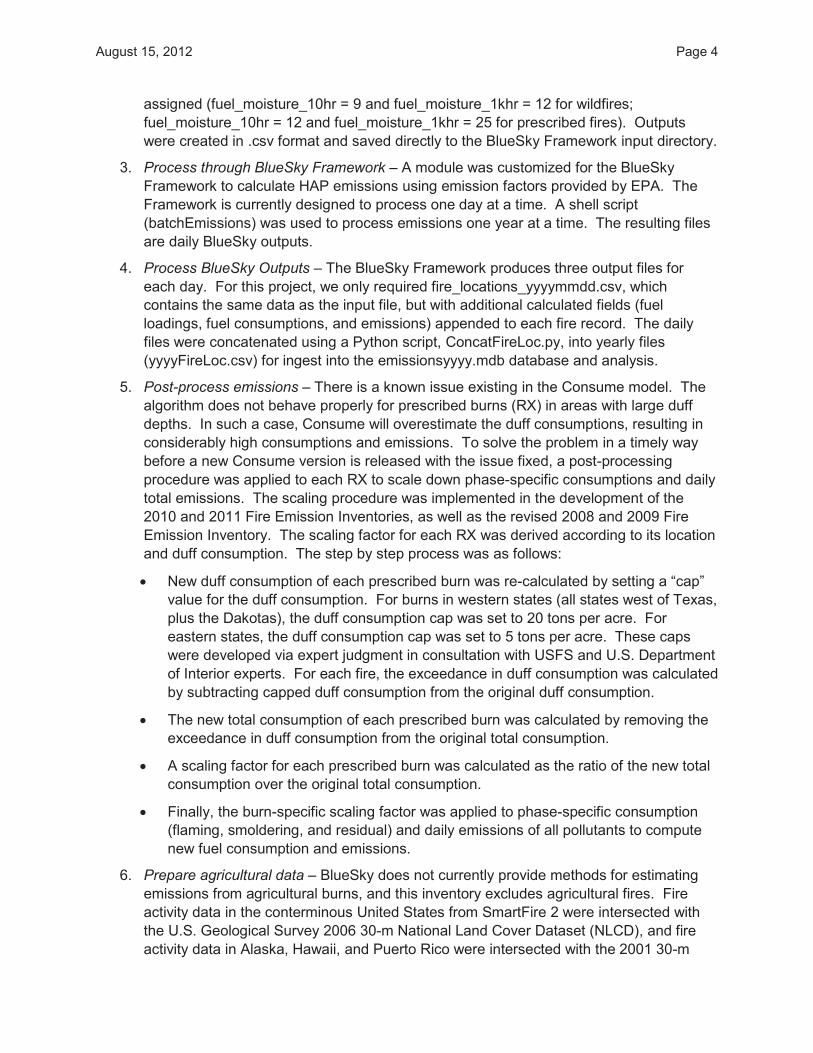
5. Post-process emissions – There is a known issue existing in the Consume model. The

algorithm does not behave properly for prescribed burns (RX) in areas with large duff

depths. In such a case, Consume will overestimate the duff consumptions, resulting in

considerably high consumptions and emissions. To solve the problem in a timely way

before a new Consume version is released with the issue fixed, a post-processing

procedure was applied to each RX to scale down phase-specific consumptions and daily

total emissions. The scaling procedure was implemented in the development of the

2010 and 2011 Fire Emission Inventories, as well as the revised 2008 and 2009 Fire

Emission Inventory. The scaling factor for each RX was derived according to its location

and duff consumption. The step by step process was as follows:

· New duff consumption of each prescribed burn was re-calculated by setting a “cap”

value for the duff consumption. For burns in western states (all states west of Texas,

plus the Dakotas), the duff consumption cap was set to 20 tons per acre. For

eastern states, the duff consumption cap was set to 5 tons per acre. These caps

were developed via expert judgment in consultation with USFS and U.S. Department

of Interior experts. For each fire, the exceedance in duff consumption was calculated

by subtracting capped duff consumption from the original duff consumption.

· The new total consumption of each prescribed burn was calculated by removing the

exceedance in duff consumption from the original total consumption.

· A scaling factor for each prescribed burn was calculated as the ratio of the new total

consumption over the original total consumption.

· Finally, the burn-specific scaling factor was applied to phase-specific consumption

(flaming, smoldering, and residual) and daily emissions of all pollutants to compute

new fuel consumption and emissions.

6. Prepare agricultural data – BlueSky does not currently provide methods for estimating

emissions from agricultural burns, and this inventory excludes agricultural fires. Fire

activity data in the conterminous United States from SmartFire 2 were intersected with

the U.S. Geological Survey 2006 30-m National Land Cover Dataset (NLCD), and fire

activity data in Alaska, Hawaii, and Puerto Rico were intersected with the 2001 30-m

August 15, 2012 Page 5

NLCD. NLCD classifies all area in the United States into one of 19 land cover types

(Figure 1). Fires that fell within land cover types 81 (Pasture/Hay) or 82 (Cultivated

Crops) were assumed to be agricultural burns and removed from the yyyyFireLoc table

to make a yearly agricultural fire table (AgActivityClean) in the emissionsyyyy.mdb

database.

7. Preparing wildland fire data – yyyyFireLoc table in the emissions.mdb database was

formatted into the final emission inventory table (WF_locations_All) after filtering out the

agricultural burn data.

The emissions processing steps 1 to 5 were omitted for Hawaii and Puerto Rico wildland

fires because the model chain used in the BlueSky Framework was different. FINN does not

require fuel moisture data, nor does it need daily fire activity input files. The activity data of fires

in Hawaii and Puerto Rico were input into the BlueSky Framework in one single file, and the

output file, fire_locations.csv, contained the fuel consumptions and emissions data for all fires in

the input file. The outputs were first post-processed to estimate VOC and HAP emissions as

described previously in the “Process Streams” section, appended to the yyyyFireLoc table in the

emissionsyyyy.mdb database, and finalized for this emissions inventory through steps 6 and 7.

Figure 1. NLCD map used to identify and segregate agricultural burns. Puerto Rico data are not shown in this figure.

August 15, 2012 Page 6

Emissions QA/QC

For the 2011 fire inventory produced with SmartFire 2, several steps were taken to QC

the data and confirm that the algorithms and datasets incorporated into SmartFire 2 worked

appropriately.

Before Running SmartFire 2:

· We reviewed input datasets and identified any data gaps that needed to be filled with

alternative data (e.g., gaps in HMS data were filled with MODIS data).

· We identified fire incidents that appeared to be double-counted in individual data sets

and removed duplicate records.

· We examined fires with long durations or conflicts between start date and report date to

identify fires that may have erroneous start dates. Start dates later than report dates

were replaced with the report dates.

· We spot-checked reported location coordinates for selected fires.

After Running SmartFire 2:

· We checked the location, duration, underlying fire activity input data, final shape, and

final size for large fire events (i.e., area burned > 10,000 acres) to ensure that the results

were reasonable.

· We checked large fire events (i.e., area burned > 10,000 acres) by state and by name

and removed duplicate events.

· We produced and reviewed summary tables and plots of the 2011 fire inventory data.

· We compared acres burned by state to National Interagency Fire Center

(http://www.nifc.gov/fireInfo/fireInfo_statistics.html) data to make sure the summary

values are within reasonable range.

Summary of 2011 Wildland Fire Emission Inventory

We estimated that, in 2011, wildland fires burned over 23 million acres in the United

States and emitted more than 2.6 million tons of PM2.5. The area burned by wild and prescribed

fires make up 43% and 57% of the total area burned, respectively. Wildfire PM2.5 emissions

account for 67% of the total emissions and prescribed burns account for 33%.

In the 2011 Wildland Fire Emission Inventory, the bulk of emissions originate from two

regions: the West and the Southeast. This concentration of emissions is consistent with

previous national fire inventories prepared by STI for EPA and can be seen in the emissions

density plot shown in Figure 2. Figure 3 depicts the total monthly PM2.5 emissions for each

state. The springtime emissions are mostly from the southeastern states, where prescribed

burning is a common land management practice in spring. The summer/fall emissions occur

primarily in the West and Southwest, particularly in California, Oregon, Arizona, and New

Mexico. Figures 4 and 5 depict the area burned per square mile by county for wildland fires

and total area burned by county for agricultural fires, as calculated by SmartFire 2.

August 15, 2012 Page 7

Figure 2. 2011 wildland fire PM2.5 emission density. Puerto Rico data are not shown in this figure.

Figure 3. 2011 total monthly PM2.5 emissions (tons) from wildland fires by state. Puerto Rico data are not shown in this figure.

August 15, 2012 Page 8

Figure 4. 2011 wildland fire area burned (acres per square mile) by county. Puerto Rico data are not shown in this figure.

Figure 5. 2011 agricultural fire total area burned (acres) by county. Puerto Rico data are not shown in this figure.

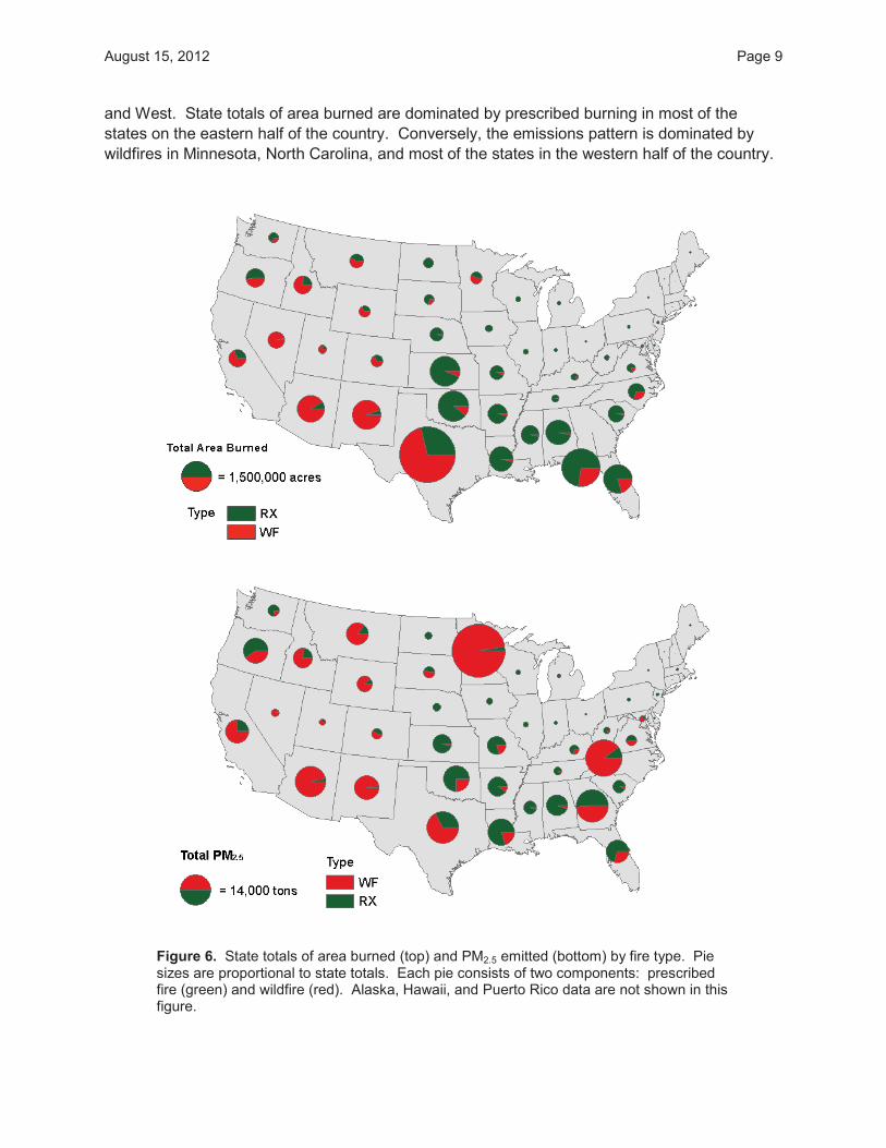
Area burned and PM2.5 results by state and fire type are presented in Figure 6. Large

totals of area burned are present throughout the Southeast, the Southern Plains, Southwest,

August 15, 2012 Page 9

and West. State totals of area burned are dominated by prescribed burning in most of the

states on the eastern half of the country. Conversely, the emissions pattern is dominated by

wildfires in Minnesota, North Carolina, and most of the states in the western half of the country.

Figure 6. State totals of area burned (top) and PM2.5 emitted (bottom) by fire type. Pie sizes are proportional to state totals. Each pie consists of two components: prescribed fire (green) and wildfire (red). Alaska, Hawaii, and Puerto Rico data are not shown in this figure.

August 15, 2012 Page 10

The monthly patterns of area burned and PM2.5 emissions are shown in Figures 7

and 8. In this inventory, the peak season for area burned is late winter/early spring, but the

peaks of PM2.5 emissions are in early summer and fall. This difference is a result of the offset

between the prescribed and wildfire burning seasons and the larger relative emissions per area

burned for wildfires. In 2011, substantial wildfire activities in the southwest (particularly Arizona

and New Mexico) and Alaska resulted in the peak of PM2.5 emissions in June. The Pains Bay

fire and Juniper Road fire in North Carolina also contributed significant emissions in June from

the smoldering of organic soil. The Pagami Creek fire in Minnesota burned from late August

through October, consumed an extensive amount of duff fuels, and in turn resulted in the

emission peak in September.

Figure 7. Monthly area burned in the United States in 2011 by fire type. Red indicates wildfires and green indicates prescribed burns.

Figure 8. Monthly PM2.5 emitted from wildland fires in the United States in 2011 by fire type. Red indicates wildfires and green indicates prescribed burns.

0.0

0.5

1.0

1.5

2.0

2.5

3.0

3.5

4.0

4.5

5.0

1 2 3 4 5 6 7 8 9 10 11 12

Are

a B

urn

ed

(m

illi

on

acr

es)

Month

WF

RX

0

50

100

150

200

250

300

350

400

450

500

1 2 3 4 5 6 7 8 9 10 11 12

PM

2.5

Em

issi

on

s (1

,00

0 t

on

s)

Month

WF

RX

August 15, 2012 Page 11

Comparison with Previous Years

The 2011 Wildland Fire Emission Inventory was compared with prior years’ inventories

developed by STI for EPA. Figure 9 displays the temporal variability in PM2.5 emissions from

wildland fires in the contiguous United States in the past five years (from 2007 to 2011). The

total wildland fire PM2.5 emissions in 2011 are within the range shown in recent years. An

apparent contrast in the temporal variability between emissions from wildfires and from

prescribed burns demonstrates that wildfire smoke emissions vary significantly from year to

year, whereas the differences in prescribed burn emissions over time change at a much smaller

magnitude. The trends acknowledge the unpredictable nature of wildfire occurrence and

indicate that the managed practice of prescribed burns takes place more or less regularly and

consistently over the years.

Figure 9. Total PM2.5 emissions from wildland fires in the contiguous United States from 2007 to 2011, separated by fire type (WF = wildfires; RX = prescribed fires).

The spatial distributions and densities of PM2.5 emissions from wildland fires in the

contiguous United States from 2007 to 2011 are illustrated in Figure 10. The emissions are

consistently concentrated in the western and southeastern states over the five-year period. As

discussed previously, prescribed burning is practiced commonly in spring in the southeastern

United States, and western states are prone to wildfires under dry conditions in summer. The

locations of large wildfires are represented by dark red spots on the maps where high amounts

of PM2.5 were emitted, and the locations are different every year.

0

500

1,000

1,500

2,000

2,500

3,000

2007 2008 2009 2010 2011

PM

2.5

Em

issi

on

s (1

,00

0 t

on

s)

Year

WF

RX

August 15, 2012 Page 12

(a) 2007

(b) 2008 (c) 2009

(d) 2010 (e) 2011

Figure 10. Annual wildland fire PM2.5 emission density in the contiguous United States estimated for year (a) 2007, (b) 2008, (c) 2009, (d) 2010, and (e) 2011.

August 15, 2012 Page 13

Deliverables

STI is providing the 2011 Wildland Fire Emission Inventory in the following formats:

· Microsoft Access files formatted identically to those prepared for the previous efforts (WA 5-17 under Contract No. EP-D-05-004 and WA 2-21 under Contract No. EP-D-09-097).

· EIS Events format, which consists of Microsoft Access-based “staging tables” that can be converted to XML format by EPA’s Consolidated Emissions Reporting Schema (CERS) XML file generator and uploaded to EIS. STI populated the Access staging tables with 2011 fire emissions data and produced separate Access databases for each state.

In addition, STI is providing all relevant daily and aggregated data and metadata in

Microsoft Access or Excel tables.

References

Pollard E.K., Du Y., Raffuse S.M., and Reid S.B. (2011) Preparation of wildland and agricultural fire emissions inventories for 2009. Technical memorandum prepared for the U.S. Environmental Protection Agency, Research Triangle Park, NC, by Sonoma Technology, Inc., Petaluma, CA, STI-910221-4231, October 6.

Wiedinmyer C., Akagi S.K., Yokelson R.J., Emmons L.K., Al-Saadi J.A., Orlando J.J., and Soja A.J. (2011) The Fire INventory from NCAR (FINN): a high resolution global model to estimate the emissions from open burning. Geosci. Model Dev. Discuss., 3, 2439-2476 (doi:10.5194/gmd-4-625-2011). Available on the Internet at http://www.geosci-model-dev.net/4/625/2011/gmd-4-625-2011.pdf.