Appendix A Complex Numbers
39
Appendix A Complex Numbers A.1 Fields A field is a set F together with two operations, called addition and multiplication and denoted by the usual symbolism, which satisfy the following conditions. A1. a + b = b + a for all a, b ∈ F A2. (a + b)+ c = a +(b + c) for all a, b, c ∈ F A3. There exists an element denoted by 0 ∈ F such that a +0= a for all a ∈ F A4. For each a ∈ F there exists an element -a ∈ F such that a +(-a)=0 M1. ab = ba for all a, b ∈ F M2. (ab)c = a(bc) for all a, b, c ∈ F M3. There exists an element denoted by 1 ∈ F such that 1a = a for all a ∈ F M4. For each 0 = a ∈ F there exists an element a -1 ∈ F such that aa -1 =1 D. a(b + c)= ab + ac for all a, b, c ∈ F It can be shown that the additive identity 0 and the multiplicative identity 1 are unique in F. Also each element a has a unique additive inverse -a, and each a =0 has a unique multiplicative inverse a -1 . The subtraction operation in F is defined in terms of addition as a - b = a +(-b) and the division operation is defined in terms of multiplication as a/b = ab -1 , b =0 Familiar examples of fields are the field of rational numbers and the field of real numbers (denoted R). Another common one is the field of complex numbers explained next. A.2 Complex Numbers A complex number is of the form z = a + ib 295
Transcript of Appendix A Complex Numbers

Appendix A
Complex Numbers
A.1 Fields
A field is a set F together with two operations, called addition and multiplication anddenoted by the usual symbolism, which satisfy the following conditions.
A1. a + b = b + a for all a, b ∈ F
A2. (a + b) + c = a + (b + c) for all a, b, c ∈ F
A3. There exists an element denoted by 0 ∈ F such that a + 0 = a for all a ∈ F
A4. For each a ∈ F there exists an element −a ∈ F such that a + (−a) = 0
M1. ab = ba for all a, b ∈ F
M2. (ab)c = a(bc) for all a, b, c ∈ F
M3. There exists an element denoted by 1 ∈ F such that 1a = a for all a ∈ F
M4. For each 0 6= a ∈ F there exists an element a−1 ∈ F such that aa−1 = 1
D. a(b + c) = ab + ac for all a, b, c ∈ F
It can be shown that the additive identity 0 and the multiplicative identity 1 areunique in F. Also each element a has a unique additive inverse −a, and each a 6= 0has a unique multiplicative inverse a−1. The subtraction operation in F is defined interms of addition as
a− b = a + (−b)
and the division operation is defined in terms of multiplication as
a/b = ab−1 , b 6= 0
Familiar examples of fields are the field of rational numbers and the field of realnumbers (denoted R). Another common one is the field of complex numbers explainednext.
A.2 Complex Numbers
A complex number is of the form
z = a + ib
295

296 Complex Numbers
where a, b ∈ R and
i2 = −1
a and b are called the real and imaginary parts of z, respectively, denoted
a = Re z , b = Im z
Two complex numbers z1 = a1 + ib1 and z2 = a2 + ib2 are called equal if a1 = a2 andb1 = b2. The addition and multiplication of z1 and z2 are defined as
z1 + z2 = (a1 + a2) + i(b1 + b2)
and
z1z2 = (a1a2 − b1b2) + i(a1b2 + a2b1)
Note that multiplication of two complex numbers is performed by the usual rules foralgebraic multiplication with i2 = −1.
Defining additive and multiplicative identities as
0 = 0 + i0 , 1 = 1 + i0
additive inverse of z = a + ib as
−z = (−a) + i(−b)
and the multiplicative inverse as
z−1 = a/(a2 + b2)− ib/(a2 + b2)
it can be shown that the set of all complex numbers C together with the aboveaddition and multiplication, is a field. Every real number can be considered as acomplex number with imaginary part equal to 0, that is a = a + i0. Its additiveinverse and multiplicative inverse (if a 6= 0) as a complex number are the same as itsadditive and multiplicative inverses as a real number. Thus R, which is itself a field,is a subfield of C with respect to the same addition and multiplication operations.
The complex conjugate of z = a + ib is defined to be
z∗ = a− ib
Note that
zz∗ = (a + ib)(a− ib) = a2 + b2
There is a geometrical representation of complex numbers. To a given complexnumber z = a + ib we associate the point in a plane with abscissa a and ordinate b,relative to a rectangular coordinate system in the plane, as shown in Figure A.1. Inthis way there is a one-to-one correspondence between the set of all complex numbersand the set of all points in the plane. The absolute value or modulus of z, is definedas
|z| =√
zz∗ = (a2 + b2)1/2

A.2 Complex Numbers 297
y
b
0
−b
a x
z = a + ib
r
r
θ−θ
z* = a − ib
= reiθ
= re−iθ
Figure A.1: Representation of a complex number
Geometrically, this is the polar distance r of the point (a, b) from the origin (0, 0),that is, |z| = r. We also define the argument of z 6= 0, denoted arg z, to be the polarangle θ shown in the figure, that is
arg z = θ = tan−1(b/a)
Note that
z = r(cos θ + i sin θ)
Using the series representations
cos θ = 1− θ2/2! + θ4/4!− · · ·sin θ = θ − θ3/3! + θ5/5!− · · ·
and rearranging the terms we observe that
cos θ + i sin θ = 1 + (iθ) + (iθ)2/2! + (iθ)3/3! + · · ·
By analogy to the series representation of the real quantity
ex = 1 + x + x2/2! + x3/3! + · · ·
the above series can conveniently be defined as eiθ. Thus we obtain
z = r(cos θ + i sin θ) = reiθ
which is called the polar representation of the complex number z. Polar representationprovides simplicity in multiplication and division of complex numbers. If z1 = r1e
iθ1
and z2 = r2eiθ2 , then
z1z2 = r1r2ei(θ1+θ2)
and if z2 6= 0 (r2 6= 0), then
z1/z2 = (r1/r2)ei(θ1−θ2)

298 Complex Numbers
A.3 Complex-Valued Functions
If f and g are real-valued functions of a real variable t, then
h(t) = f(t) + ig(t)
defines a complex-valued function h of t. If f and g are differentiable on an intervala < t < b, then h is also differentiable, and its derivative is given by
h′(t) = f ′(t) + ig′(t)
A useful complex-valued function is ezt, where z = a + ib is a complex numberand t is a real variable. Using the polar representation, ezt can be expressed as
ezt = e(a+ib)t = eateibt = eat(cos bt + i sin bt)
Differentiating real and imaginary parts of ezt, and rearranging the terms we get
d
dtezt = aeat(cos bt + i sin bt) + eat(−b sin bt + ib cos bt)
= eat(a cos bt− b sin bt) + ieat(a sin bt + b cos bt)
= (a + ib)eat(cos bt + i sin bt)
= zezt
Thus the usual differentiation property of the real-valued exponential function is gen-eralized to the complex-valued exponential function.

Appendix B
Existence and Uniqueness
Theorems
Consider a system of first order ordinary differential equations together with a set ofinitial conditions:
x′ = f(x, t) , x(t0) = xo (B.1)
where f : Rn×1×R→ R
n×1 is a vector-valued function defined on some interval I ⊂ R
containing t0. We assume that
a) for every fixed x ∈ Rn×1, the function f(x, ·) : t→ f(x, t) is piecewise continu-
ous on I, and
b) f satisfies a Lipschitz condition on I, that is, there exists a constant K > 0such that 1
‖ f(x1, t)− f(x2, t) ‖ ≤ K‖x1 − x2 ‖ (B.2)
for all x1,x2 ∈ Rn×1 and t ∈ I.
Recall that a vector-valued function φ defined on I is called a solution of (B.1) ifφ(t0) = xo and
φ′(t) = f(φ(t), t) (B.3)
at all continuity points of f . Clearly, if φ is a solution, then integrating both sides of(B.3) from t0 to t, we obtain
φ(t) = x0 +
∫ t
t0
f(φ(τ), τ) dτ (B.4)
Conversely, if φ satisfies the integral equation in (B.4), then it is a solution of (B.1).We will use this fact in the proof of the following existence and uniqueness theorem.
Theorem B.1 Under the assumptions (a) and (b) above, the initial-value problemin (B.1) has a unique, continuous solution on I.
1The Lipschitz condition in (B.2) is stronger than continuity of f in x. For example, the scalarfunction f(x, t) =
√x defined on I = [0,∞) is continuous everywhere on I, but does not satisfy a
Lipschitz condition. With x1 = x and x2 = 0, there exists no K that satisfies
√x ≤ Kx
for all x ≥ 0.
299
300 Existence and Uniqueness Theorems
Proof Define a sequence of continuous functions recursively as
φ0(t) = x0
φm(t) = x0 +
∫ t
t0
f(φm−1(τ ), τ ) dτ , m = 1, 2, . . . (B.5)
Fix T > 0 such that J = [t0, t0 + T ] ⊂ I. Since f(x0, t) is piecewise continuous, it isbounded on J . Let
B = maxt∈J
{ f(x0, t) }
We claim that
‖φm(t)− φm−1(t) ‖ ≤B
K
Km(t− t0)m
m!, m = 1, 2, . . . (B.6)
for all t ∈ J . The claim is true for m = 1 as
‖φ1(t)− φ0(t) ‖ ≤ ‖
∫ t
t0
f(φ0(τ ), τ ) dτ ‖ ≤
∫ t
t0
‖ f(x0, τ ) ‖ dτ ≤ B(t− t0)
Suppose it is true for m = k. Then for m = k + 1
‖φk+1(t)− φk(t) ‖ ≤ ‖
∫ t
t0
[ f(φk(τ ), τ )− f(φk−1(τ ), τ ) ] dτ ‖
≤
∫ t
t0
K ‖φk(τ )− φk−1(τ ) ‖ dτ
≤
∫ t
t0
KB
K
Kk(τ − t0)k
k!dτ
≤B
K
Kk+1(t− t0)k+1
(k + 1)!
so that it is also true for m = k + 1. Hence it is true for all m ≥ 1. Since t− t0 ≤ T forall t ∈ J , (B.6) further implies that
‖φm(t)− φm−1(t) ‖ ≤B
K
(KT )m
m!, m = 1, 2, . . .
Define
φm(t) = ‖φm(t)− φ0(t) ‖
Then
φm(t) = ‖
m∑
k=1
[φk(t)− φk−1(t) ] ‖ ≤
m∑
k=1
‖φk(t)− φk−1(t) ‖
≤B
K
m∑
k=1
(KT )k
k!≤
B
K(eKT − 1) , m = 1, 2, . . .
for all t ∈ J . This implies that the sequence of nonnegative-valued continuous func-tions {φm } converges uniformly on J .2 Consequently, the sequence of vector-valuedcontinuous functions {φm } converges uniformly to a continuous limit function φ.3
2This is a direct consequence of the comparison test. For details the reader is referred to a bookon advanced calculus.
3That is, given any ε > 0, there exist M > 0 such that
‖φ(t) − φm(t) ‖ ≤ ε
for all m ≥ M and for all t ∈ J .

B.1 Existence and Uniqueness Theorems 301
Uniform convergence of {φm }, together with the Lipschitz condition on f furtherimply that
a) limm → ∞
f(φm(t), t) = f(φ(t), t)
b) limm → ∞
∫ t
t0
f(φm(τ ), τ ) dτ =
∫ t
t0
f(φ(τ ), τ ) dτ
Thus
φ(t) = limm → ∞
φm(t)
= xo + limm → ∞
∫ t
t0
f(φm−1(τ ), τ ) dτ
= xo +
∫ t
t0
f(φ(τ ), τ ) dτ
for all t ∈ J , proving that φ is a solution of (B.1) on J .To prove uniqueness of φ, suppose (B.1) has another solution ψ on J . Define
g(t) = ‖φ(t)− ψ(t) ‖ = ‖
∫ t
t0
[ f(φ(τ ), τ )− f(ψ(τ ), τ ) ] dτ ‖
Then
g(t) ≤
∫ t
t0
‖ f(φ(τ ), τ )− f(ψ(τ ), τ ) ‖ dτ ≤
∫ t
t0
Kg(τ ) dτ
for all t ∈ J . Let
h(t) = e−K(t−t0)
∫ t
t0
Kg(τ ) dτ
Then h(t0) = 0 and
h′(t) = Ke
−K(t−t0)[ g(t)−
∫ t
t0
Kg(τ ) dτ ] ≤ 0
so that
h(t) ≤ 0 for all t ∈ J
Hence
0 ≤ g(t) ≤
∫ t
t0
Kg(τ ) dτ ≤ 0 for all t ∈ J
This implies g(t) = 0 for all t ∈ J , or equivalently,
φ(t) = ψ(t) for all t ∈ J
contradicting the assumption that φ and ψ are two different solutions on J . In conclu-sion, (B.1) has a unique solution on J .
The case t < t0 can be analyzed similarly by considering a closed interval J =
[t0 − T, T ] ⊂ I. Since T is arbitrary in both cases, it follows that (B.1) has a unique,
continuous solution on I.

302 Existence and Uniqueness Theorems
The functions in (B.5) that converge to the solution of (B.1) are known as thePicard iterates, and provide a constructive method for the proof of the existenceof a solution. The proof of the uniqueness part of the theorem is a variation of thewell-known Bellman-Gronwal Lemma.
Proof of Theorem 6.1
The proof follows immediately from Theorem B.1 on noting that
f(x, t) = A(t)x + u(t)
is piecewise continuous for every fixed x ∈ Rn×1, and satisfies a Lipschitz condition with
K = supt∈I
‖A(t)‖

Appendix C
The Laplace Transform
C.1 Definition and Properties
The one-sided (or unilateral) Laplace transform of a real- or complex-valued func-tion f of a real variable t is a complex-valued function F of a complex variable s,defined by
F (s) =
∫
∞
0
f(t)e−st dt (C.1)
provided the integral converges. For convenience, the Laplace transform of f is alsodenoted by L{f}.
Let f be a piece-wise continuous function that is bounded by an exponential, thatis, there exist M, α ∈ R such that
|f(t)| ≤Meαt
holds for all t. Such a function is said to be of exponential order α. Then for anys = σ + iω ∈ C with σ > α
|∫
∞
0
f(t)e−st dt | ≤∫
∞
0
|f(t)e−st| dt
≤∫
∞
0
Me(α−σ)t dt
≤ M
σ − α
and thus the integral in (C.1) converges. The region
Cα = { s = σ + iω |σ > α }
is called the region of convergence of F .
Let f be a function of exponential order α with a Laplace transform F (s) thatexists in a region Cα, and suppose that f(t) = 0 for t < 0. Then f can be obtaineduniquely from F by means of a line integral as
f(t) = limω → ∞
∫
Γ
F (s)est ds (C.2)
303

304 The Laplace Transform
where Γ is a vertical straight line in Cα extending from s = σ− iω to s = σ + iω. Theintegral on the right-hand side of (C.2) is called the inverse Laplace transform ofF , denoted by L−1(F ).1 We use the notation
f(t) ←→ F (s)
to indicate that f and F are a Laplace transform-inverse Laplace transform pair.Some useful properties of the Laplace transform are stated below, where it is
assumed that the Laplace transforms involved exist.
a) Linearity
af(t) + bg(t) ←→ aF (s) + bG(s)
b) Shift
f(t− t0) ←→ e−st0F (s) , t0 > 0
es0tf(t) ←→ F (s− s0) , s0 ∈ C
c) Scaling
f(at) ←→ 1
aF (
s
a) , a > 0
d) Differentiation
f (n)(t) ←→ snF (s)− sn−1f(0)− · · · − sf (n−2)(0)− f (n−1)(0)
tnf(t) ←→ (−1)n dn
dsn F (s)
The first three of the properties above are direct consequences of the definition.For example, the Laplace transform of the shifted function f(t− t0) is
∫
∞
0
f(t− t0)e−st dt =
∫
∞
−t0
f(τ)e−s(τ+t0) dτ
= e−st0
∫
∞
0
f(τ)e−sτ dτ = e−st0F (s)
proving the first property in (b).2 Proofs of the properties in (d) require some ma-nipulations. Evaluating the integral in (C.1) written for f ′ by parts, we obtain
L{f ′} =
∫
∞
0
f ′(t)e−st dt
= [ f(t)e−st ]t=∞
t=0 +
∫
∞
0
f(t)se−st dt
= sF (s)− f(0)
1In practice, the line integral in (C.2) is seldom used to find the inverse Laplace transform.Instead, Laplace transform tables are used for most of the functions of interest.
2The second equality follows from the assumption that f(t) = 0 for t < 0.

C.2 Laplace Transform Pairs 305
proving the first property in (d) for n = 1.3 The case n > 1 and the second propertyin (d) can be proved similarly.
Example C.1
The Laplace transform of the unit step function
u(t) =
{
1, t > 00, t < 0
is
U(s) =
∫ t
0
e−st
dt = [−se−st ]t=∞
t=0 =1
s, Re s > 0
By property (b),
u(t− t0) ←→e−st0
s, Re s > 0
and, by property (d)
tu(t) ←→ −d
ds(
1
s) =
1
s2
C.2 Some Laplace Transform Pairs
The Laplace transform of the unit step function obtained in Example C.1, togetherwith the properties listed in the previous section, allows us to obtain the Laplacetransform of many useful functions. For example, from the second property in (b),we obtain
eσ0tu(t) ←→ 1
s− σ0
and from property (d),
teσ0tu(t) ←→ 1
(s− σ0)2
The Laplace transform of es0tu(t), in turn, can be used to find Laplace transformsof sine and cosine functions. On noting that
eiω0tu(t) = cosω0t + i sinω0t
we obtain
(cosω0t + i sinω0t)u(t) ←→ 1
s− iω0=
s + iω0
s2 + ω20
Thus
(cosω0t)u(t) ←→ s
s2 + ω20
3Since f is exponential order α and Re s > α
limt → ∞
f(t)e−st = 0
306 The Laplace Transform
and
(sin ω0t)u(t) ←→ ω0
s2 + ω20
A list of some Laplace transform pairs, which can be derived similarly, is given inTable C.1.
C.3 Partial Fraction Expansions
A function F that is expressed as a ratio of two polynomials is called a rational
function. A rational function
F (s) =c(s)
d(s)=
c0sm + c1s
m−1 + · · ·+ cm
sn + d1sn−1 + · · ·+ dn
(C.3)
is said to be proper if m ≤ n and strictly proper if m < n.The Laplace transforms in Table C.1 are simple strictly proper rational functions
with denominators being first or second degree polynomials or powers of such poly-nomials. This observation suggests that if a rational function F can be expressed as alinear combination of such simple rational functions, then by linearity of the Laplacetransform, the inverse Laplace transform of F can be obtained as the same linearcombination of the inverse Laplace transforms of individual functions, which can bewritten down directly from the table. For example, the inverse Laplace transform of
s + 2
s2 + s=
2
s− 1
s + 1
can be written down using Table C.1 as
L−1{ s + 2
s2 + s} = (2− e−t)u(t)
Consider a strictly proper rational function F (s) expressed as in (C.3). Supposethat the denominator polynomial d(s) is factored out as
d(s) =k
∏
i=1
(s− pi)ni
where pi ∈ C are distinct zeros of d with multiplicities ni, i = 1, . . . , k. pi are calledthe poles of F . Then F can be expressed as
F (s) =
k∑
i=1
ni∑
j=1
rij
(s− pi)j (C.4)
where rij ∈ C. This expression is known as the partial fraction expansion of F .The coefficients rij can be obtained by collecting the terms on the right-hand side of(C.4) over the common denominator d and equating the coefficients of the resultingnumerator polynomial to those of c.
MATLAB provides a built-in function, residue, to compute pi and rij . Thecommands

C.3 Partial Fraction Expansions 307
Table C.1: Some Laplace transform pairs
f(t) F (s)
11
s
tnn!
sn+1
eσ0t 1
s− σ0
tneσ0t n!
(s− σ0)n+1
cosω0ts
s2 + ω20
sinω0tω0
s2 + ω20
t cosω0ts2 − ω2
0
(s2 + ω20)
2
t sinω0t2ω0s
(s2 + ω20)
2
eσ0t cosω0ts− σ0
(s− σ0)2 + ω2
0
eσ0t sin ω0tσ0
s− σ0)2 + ω2
0
teσ0t cosω0t(s− σ0)
2 − ω20
((s− σ0)2 + ω2
0)2
teσ0t sin ω0t2ω0(s− σ0)
((s− σ0)2 + ω2
0)2

308 The Laplace Transform
>> c=[c0 c1 ... cm]; d=[1 d1 ... dn];
>> [r,p]=residue(c,d);
return the poles pi in the array p (with each pole appearing as many times as itsmultiplicity) and the coefficients rij in the array r.
Example C.2
The strictly proper rational function
F (s) =2s
2 + 4s + 1
s3 + 4s
2 + 5s + 2=
2s2 + 4s + 1
(s + 2)(s + 1)2
has the poles p1 = −2 with n1 = 1 and p2 = −1 with n2 = 2. Hence F has a partialfraction expansion of the form
F (s) =r1
s + 2+
r21
s + 1+
r22
(s + 1)2
Reorganizing the above expression, we get
F (s) =r1(s + 1)2 + r21(s + 1)(s + 2) + r22(s + 2)
(s + 2)(s + 1)2(s + 2)
=(r1 + r21)s
2 + (2r1 + 3r21 + r22)s + (r1 + 2r21 + 2r22)
s3 + 4s
2 + 5s + 2
=2s
2 + 4s + 1
s3 + 4s
2 + 5s + 2
Equating the coefficients of the numerators of the last two expressions we obtain a systemof three equatins in three unknows
[
1 1 02 3 11 2 2
][
r1
r21
r22
]
=
[
241
]
the unique solution of which is easily computed as r1 = r12 = 1, r22 = −1.
Alternatively, the MATLAB commands
>> c=[2 4 1]; d=[1 4 5 2];
>> [r,p]=residue(c,d);
produce
r = [ 1 1 − 1 ] , p = [−2 − 1 − 1 ]
Note that the coefficients rij associated with a multiple pole pi appear in the order ofincreasing j in the array r.
Thus
F (s) =1
s + 2+
1
s + 1−
1
(s + 1)2
and its inverse Laplace transform is
f(t) = (e−2t + e−t − te
−t)u(t)

C.4 Solution of DEs by Laplace Transform 309
Example C.3
To find the inverse Laplace transform of
G(s) =s2 + 9s + 16
s3 + 5s
2 + 9s + 5
we execute the MATLAB commands
>> c=[1 9 16]; d=[1 5 9 5];
>> [r,p]=residue(c,d)
which compute
r = [−1.5− i − 1.5 + i 4 ] , p = [−2 + i − 2− i − 1 ]
Thus
G(s) =−1.5− i
s + 2− i+−1.5 + i
s + 2 + i+
4
s + 1
and
g(t) = (−1.5− i) e(−2+i)t + (−1.5 + i) e
(−2−i)t + 4 e−t
= 2Re { (−1.5− i) e(−2+i)t }+ 4 e
−t
= e−2t(2 sin t− 3 cos t) + 4 e
−t
C.4 Solution of Differential Equations by Laplace
Transform
Consider an nth order linear differential equation with constant coefficients
y(n) + a1y(n−1) + · · ·+ an−1y
′ + any = u(t) (C.5)
together with a set of n initial conditions
y(0) = y0 , y′(0) = y1 , . . . , y(n−1)(0) = yn−1
specified at t0 = 0. Taking the Laplace transform of both sides of (C.5) and using thedifferentiation property, we obtain
snY (s)− sn−1y0 − · · · − syn−2 − yn−1 +sn−1Y (s)− · · · − syn−3 − yn−2 +
...sY (s)− y0 +
Y (s) = U(s)
Rearranging the terms, the above expression can be written as
Y (s) =b(s)
a(s)+
1
a(s)U(s) (C.6)
where
a(s) = sn + a1sn−1 + · · ·+ an
b(s) = y0sn−1 + (y0 + y1)s
n−2 + · · ·+ (y0 + y1 + · · ·+ yn−1)

310 The Laplace Transform
Taking the inverse Laplace transform of (C.6), the solution of the given initial-valueproblem is obtained as
y = yo(t) + yu(t) , t ≥ 0 (C.7)
where
yo(t) = L−1{ b(s)
a(s)}
is part of the solution due to the initial conditions, and
yu(t) = L−1{ 1
a(s)U(s) }
is the part due to the forcing term. Note the similarity between the expressions in(2.15) and (C.7).
Example C.4
Consider the differential equation
y′′ + 2y
′ + 26y = 26u(t) , y(0) = y′(0) = 0
where u(t) is the unit step function.Taking the Laplace transforms of both sides of the given differential equation and
rearranging the terms, we get
Y (s) = Φ(s) =26
s(s2 + 2s + 26)(C.8)
Expanding Y (s) into partial fractions, we obtain
Y (s) =26
s(s + 1− 5i)(s + 1 + 5i)
=1
s+−0.5 + 0.1 i
s + 1− 5i+−0.5− 0.1 i
s + 1 + 5i
Thus
y = φ(t) = 1 + (−0.5 + 0.1 i) e(−1+5i)t + (−0.5− 0.1 i) e
(−1−5i)t
= 1 + 2Re { (−0.5 + 0.1 i) e(−1+5i)t }
= 1− e−t(cos 5t + 0.2 sin 5t) , t ≥ 0 (C.9)
the plot of which is shown in Figure C.1.If the initial conditions were specified as y(0) = 1, y′(0) = 0, then the Laplace
transform would yield
s2Y (s)− s + 2sY (s)− 2 + 26Y (s) =
26
s
or equivalently,
Y (s) =1
s
Then the solution would be
y = 1 , t ≥ 0

C.4 Solution of DEs by Laplace Transform 311
0 2 4 60
0.5
1
1.5
2 y
t
Figure C.1: Solution of the DE in Example C.4
Example C.5
Consider the same differential equation in the previous example with a different forcingfunction:
y′′ + 2y
′ + 26y = 26f(t) , y(0) = y′(0) = 0
where
f(t) =
{
1, 0 < t < 2
0, t < 0 or t > 2
is a pulse of unit strength extending from t = 0 to t = 2.Observing that
f(t) = u(t)− u(t− 2)
we have
F (s) = U(s)− e−2s
U(s) =1− e
−2s
s
Then the Laplace transform of the solution is obtained as
Y (s) =26(1− e
−2s)
s(s2 + 2s + 26)= (1− e
−2s)Φ(s)
where Φ(s) is given by (C.8). Taking the inverse Laplace transform, we compute thesolution as
y = φ(t)u(t)− φ(t− 2)u(t− 2)
=
{
φ(t), 0 < t < 2
φ(t)− φ(t− 2), t > 2
=
1− e−t(cos 5t + 0.2 sin 5t), 0 < t < 2
−e−t(cos 5t + 0.2 sin 5t)+
e−(t−2)(cos 5(t− 2) + 0.2 sin 5(t− 2)), t > 2
The solution is plotted in Figure C.2.
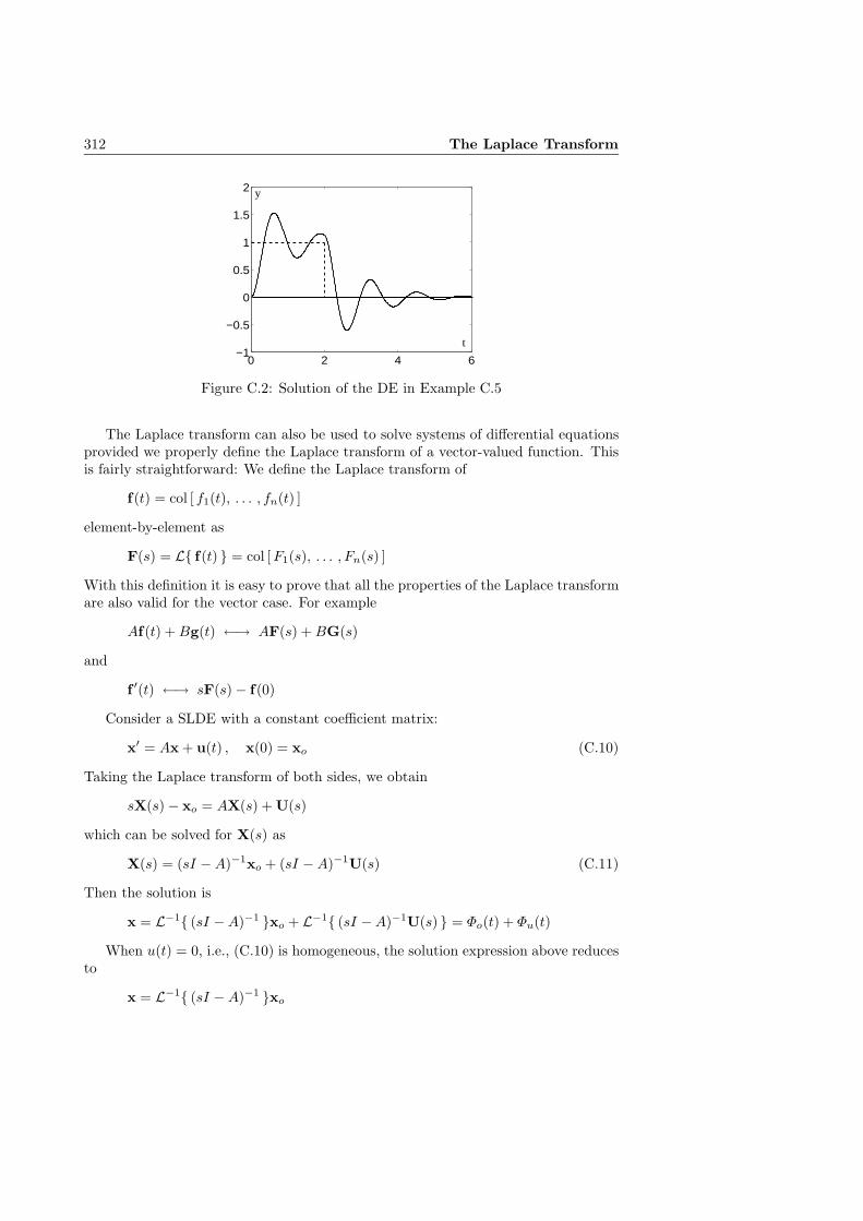
312 The Laplace Transform
0 2 4 6−1
−0.5
0
0.5
1
1.5
2 y
t
Figure C.2: Solution of the DE in Example C.5
The Laplace transform can also be used to solve systems of differential equationsprovided we properly define the Laplace transform of a vector-valued function. Thisis fairly straightforward: We define the Laplace transform of
f(t) = col [ f1(t), . . . , fn(t) ]
element-by-element as
F(s) = L{ f(t) } = col [ F1(s), . . . , Fn(s) ]
With this definition it is easy to prove that all the properties of the Laplace transformare also valid for the vector case. For example
Af(t) + Bg(t) ←→ AF(s) + BG(s)
and
f ′(t) ←→ sF(s)− f(0)
Consider a SLDE with a constant coefficient matrix:
x′ = Ax + u(t) , x(0) = xo (C.10)
Taking the Laplace transform of both sides, we obtain
sX(s)− xo = AX(s) + U(s)
which can be solved for X(s) as
X(s) = (sI −A)−1xo + (sI −A)−1U(s) (C.11)
Then the solution is
x = L−1{ (sI −A)−1 }xo + L−1{ (sI −A)−1U(s) } = Φo(t) + Φu(t)
When u(t) = 0, i.e., (C.10) is homogeneous, the solution expression above reducesto
x = L−1{ (sI −A)−1 }xo

C.4 Solution of DEs by Laplace Transform 313
Comparing the above expression with (6.19) we observe that
L−1{ (sI −A)−1 } = eAt
We thus obtain an alternative formula to compute the matrix exponential functioneAt.
Example C.6
Consider again Example 6.4, where
(sI −A)−1 =
[
s + 3 21 s + 2
]−1
=1
(s + 1)(s + 4)
[
s + 2 −2−1 s + 3
]
We can compute eAt by taking the inverse Laplace transform of the elements of(sI − A)−1 after expanding each of them into its partial fractions. However, a moreelegant approach is to expand the matrix rational function (sI − A)−1 into its partialfractions as
(sI −A)−1 =1
s + 1R1 +
1
s + 4R2
=1
(s + 1)(s + 4)[(s + 4)R1 + (s + 1)R2]
=1
(s + 1)(s + 4)[(R1 + R2)s + (4R1 + R2)]
Comparing the numerator polynomial matrices of the two expressions for (sI−A)−1, weget
R1 + R2 =
[
1 00 1
]
4R1 + R2 =
[
2 −2−1 3
]
from which we obtain
R1 =1
3
[
1 −2−1 2
]
, R2 =1
3
[
2 21 1
]
Thus
eAt = e
−tR1 + e
−4tR2 =
1
3
[
e−t + 2e−4t −2e−t + 2e−4t
−e−t + e−4t 2e−t + e−4t
]
and the solution corresponding to the given initial condition xo = col [ 1, 2 ] is
x = eAt
xo =
[
−e−t + 2e−4t
e−t + e−4t
]
which is the same as the one obtained in Example 6.4.Of course, we can obtain the solution corresponding to a given initial condition di-
rectly without computing eAt. By computing X(s) and expanding it into partial fractionsas
X(s) = (sI −A)−1xo =
1
(s + 1)(s + 4)
[
s + 2 −2−1 s + 3
][
12
]
=1
(s + 1)(s + 4)
[
s− 22s + 5
]
=1
s + 1
[
−11
]
+1
s + 4
[
21
]
we get the same solution.

314 The Laplace Transform

Appendix D
A Brief Tutorial on MATLAB
MATLAB is an interactive system and a programming language for general scientificand technical computation. When it is invoked (either by clicking on the Matlabicon or by typing the command matlab from the keyboard) the command prompt >>appears indicating that MATLAB is ready to accept command from the keyboard.Commands are terminated by “return” or “enter” keys. The exit or quit commandends MATLAB.
D.1 Defining Variables
The basic data element of MATLAB is a matrix that does not require dimensioning.Scalars and arrays (vectors) are treated as special matrices. A variable is a dataelement with a name, which can be any combination of upper and lowercase letters,digits and underscores, starting with a letter and length not exceeding 19. Variablesare case sensitive, so A and a are different variables.
Variables are assigned numerical values by typing an expression or a formula or afunction that utilizes arithmetic operations on numerical data or previously definedvariables. For example, the commands
>> a=2+7; b=4*a;
>> c=sqrt(b);
assign the values 9, 36 and 6 to the variables a, b and c, respectively; and the command
>> c=c/3;
reassigns c the value 2. Note that more than one command, separated by commas orsemicolons, may appear on a single line. When a command is not terminated by asemicolon the result of the operation is echoed on the screen:
>> d=sin(pi/c)
d =
1
If the result of an operation is not assigned to a variable, it is assigned to a defaultvariable ans (short for “answer”):
>> a+sqrt(-b)
ans =
9.0000+6.0000i
The last example shows that MATLAB requires no special handling of complexnumbers. In fact, the imaginary unit i is one of the special variables of MATLAB.Some others are j (same as i), ans (default variable name), pi (π), eps (smallest
315

316 A Brief Tutorial on MATLAB
number such that when added to 1 creates a floating-point number greater than 1),inf (∞) and NaN (not a number, e.g., 0/0). It is recommended that these variablesshould not be used as variable names to avoid changing their values.
A matrix is defined by entering its elements row by row as
>> A=[1 2 3 4; 3 4 5 6; 5 6 7 8]
A =
1 2 3 4
3 4 5 6
5 6 7 8
where elements in each row are separated by spaces (or commas), and the rows bysemicolons. Thus the commands
>> x=[2 4 6 8]; y=[-3; 2; -1];
define a row vector x, and a column vector y. In particular, the command
start:increment:end
generates a row vector (an array) of equally spaced values with the values of startand end specifying the first and the last elements of the array. If the increment isomitted, it is assumed to be 1. Thus
>> arry=-3:2:9
arry =
-3 -1 1 3 5 7 9
Note also:
>> B(1,2)=7, B(2,4)=2
B =
0 7
B =
0 7 0 0
0 0 0 2
The command size(A) returns a 1 × 2 row vector consisting of the number ofrows and the number of columns of A. For a row or column vector x, the commandlength(x) returns the number of elements of the vector. Thus
>> size(A), size(arry), length(arry)
ans =
3 4
ans =
1 7
ans =
7
A particular element of a matrix (or a row or column vector) can be extracted as
>> a23=A(2,3), x3=x(3), x3new=x(1,3), y2=y(2)
a23 =
5
x3 =
6

D.1 Defining Variables 317
x3new =
6
y2 =
2
To extract a submatrix of a matrix, the rows and columns of the submatrix arespecified:
>> sub1=A(2,3:4), sub2=A([1 3],[2 3]), sub3=A(2,:)
sub1 =
5 6
sub2 =
2 3
6 7
sub3 =
3 4 5 6
Thus sub1 consists of row 2 and columns 3 and 4 of A, sub2 rows 1 and 3 and columns2 and 3, and sub3 row 2 and all columns. Similarly,
>> part=arry(2:5)
part =
-1 1 3 5
Conversely, a matrix can be constructed from smaller blocks:
>> A1=[x;0:3], A2=[A y A(:,[3 1])]
A1 =
2 4 6 8
0 1 2 3
A2 =
1 2 3 4 -3 3 1
3 4 5 6 2 5 3
5 6 7 8 -1 7 5
MATLAB has special commands for generating special matrices: eye(n) generatesan identity matrix of order n, zeros(m,n) an m×n zero matrix, ones(m,n) an m×nmatrix with all elements equal to 1. If d is a row or column matrix of length n,the command diag(d) generates an n × n diagonal matrix with the elements of dappearing on the diagonal; and if A is an m × n matrix, diag(A) gives a columnvector of the diagonal elements of A.
All commands entered and variables defined in a session are stored in MATLAB’sworkspace, and can be recalled at any time. Typing the name of a variable returnsits value:
>> A1
A1 =
2 4 6 8
0 1 2 3
The command who gives a list of all variables defined.
>> who
Your variables are:

318 A Brief Tutorial on MATLAB
A a c sub2 x3new
A1 a23 d sub3 y
A2 arry part x y2
B b sub1 x3
The command clear v_name_1 v_name_2 clears the variables v_name_1 and v_name_2
from the workspace, and clear clears all variables.The command save fn saves the workspace in the binary file fn.mat, which can
later be retrieved by the load fn command. Menu items Save Workspace As... andLoad Workspace in the File menu serve the same purpose.
D.2 Arithmetic Operations
MATLAB utilizes the following arithmetic operators: + (addition), - (subtraction), *(multiplication), ^ (power operator), ’ (transpose), / and \ (right and left division).
These operators work on scalars or matrices:
>> i*sub1, (sub1-[8 5])*sub2
ans =
0+5.0000i 0+6.0000i
ans =
0 -2
where * denotes a scalar multiplication in the first command and matrix multiplicationin the second. However,
>> sub2*sub1
??? Error using ==> *
Inner matrix dimensions must agree.
which indicates that the matrices are not compatible for the product.Although addition of matrices requires that the matrices be of the same order,
for convenience MATLAB also allows for addition of a scalar and a matrix by firstenlarging the scalar to the size of the matrix. Thus
>> sub2+2
ans =
4 5
8 9
that is, sub2+2 is equivalent to sub2+2*ones(2,2).The power operator requires a square matrix as operand:
>> C=[0 i; -i 0]^3
C =
0 0+1.0000i
0-1.0000i 0
The transpose operator takes the Hermitian adjoint of a matrix, which reduces totranspose when the matrix is real. Thus
>> [1-i;2+i]’
ans =
1.0000+1.0000i 2.0000-1.0000i

D.2 Arithmetic Operations 319
Right division operator / works as usual when both operands or the divisor is ascalar:
>> C/5
ans =
0 0+0.2000i
0-0.2000i 0
However, care must be taken when “dividing” two matrices: The command A/B cal-culates a matrix Y such that A=YB. Obviously, this requires that A and B have the samenumber of columns. If the equation is inconsistent then Y is a least-squares solution.Thus
>> [0 2]/[1 2; 3 4]
ans =
3 -1
calculates the exact solution of the consistent equation
[ 0 2 ] = Y
[
1 23 4
]
and
>> [2 4]/[6 2]
ans =
0.5000
calculates a least-squares solution of the inconsistent equation
[ 2 4 ] = Y [ 6 2 ]
Similarly, the command A\B (left division) calculates a matrix X such that AX=B,provided that A and B have the same number of rows. Again, if the equation isinconsistent then X is a least-squares solution. Thus
>> [1 2; 3 4]\[0 2]
ans =
2.0000
-1.0000
Note that A\B = (B’/A’)’.MATLAB also provides array versions of the above arithmetic operators that allow
for element-by-element operations on arrays (row or column vectors). If x and y arearrays of the same length, then x.*y generates an array whose elements are obtainedby multiplying corresponding elements of x and y. Array versions of right and leftdivision and the power operator are defined similarly. For example,
>> x=[1 2 3]; y=[4 5 6];
>> x.*y
ans =
4 10 18
>> x./y, x.\y
ans =
0.2500 0.4000 0.5000

320 A Brief Tutorial on MATLAB
ans =
4.0000 2.5000 2.0000
>> x./2, 2./x, x.\2
ans =
0.5000 1.0000 1.5000
ans =
2.0000 1.0000 0.6667
ans =
2.0000 1.0000 0.6667
>> x.^y, y.^x
ans =
1 32 729
ans =
4 25 216
Array version of transpose operator takes the transpose (without conjugate) sothat
>> [1-i; 2+3i].’
ans =
1.0000-1.0000i 2.0000+3.0000i
D.3 Built-In Functions
MATLAB provides a number of elementary math functions that operate on individualelements of matrices. Among them are trigonometric, inverse trigonometric, hyper-bolic, inverse hyperbolic, exponential, natural and common logarithmic functions,square root, absolute value, angle, conjugate, real and imaginary parts of complexnumbers. For example,
>> u=(pi/4)*[1 -3];
>> v=sin(u)
v =
0.7071 -0.7071
>> w=sqrt(v)
w =
0.8409 0+0.8409i
>> z=exp(w)
z =
2.3184 0.6668+0.7452i
>> ang=(180/pi)*angle(w)
ang =
0 90
MATLAB also provides many useful matrix functions, some of which are summa-rized below.
>> A=[1 2 3 4; 2 3 4 5; 3 5 7 9];

D.3 Built-In Functions 321
>> rank(A)
ans =
2
>> rref(A) % reduced row echelon form
ans =
1 0 -1 -2
0 1 2 3
0 0 0 0
>> norm(A,1), norm(A,2), norm(A,inf) % p norms
ans =
18
ans =
15.7403
ans =
24
>> % singular value decomposition: A=USV’
>> [U,S,V]=svd(A)
U =
0.3472 0.7390 0.5774
0.4664 -0.6702 0.5774
0.8136 0.0688 -0.5774
S =
15.7403 0 0 0
0 0.4921 0 0
0 0 0.0000 0
V =
0.2364 -0.8026 0.3025 -0.4566
0.3914 -0.3831 -0.0629 0.8343
0.5465 0.0364 -0.7815 -0.2987
0.7016 0.4558 0.5420 -0.0790
The following matrix functions operate on square matrices:
>> A=[0 -3 1; 1 4 -2; 1 2 0];
>> det(A)
ans =
4
>> inv(A)
ans =
1.0000 0.5000 0.5000
-0.5000 -0.2500 0.2500
-0.5000 -0.7500 0.7500
>> % LU decomposition: L*U=P*A
>> [L,U,P]=lu(A)
L =

322 A Brief Tutorial on MATLAB
1.0000 0 0
0 1.0000 0
1.0000 0.6667 1.0000
U =
1.0000 4.0000 -2.0000
0 -3.0000 1.0000
0 0 1.3333
P =
0 1 0
1 0 0
0 0 1
>> % modal matrix and diagonal form: A*P=P*D
>> [P,D]=eig(A)
P =
0.5000+0.5000i 0.5000-0.5000i 0.7845
0-0.5000i 0+0.5000i -0.5883
0-0.5000i 0+0.5000i -0.1961
D =
1.0000+1.0000i 0 0
0 1.0000-1.0000i 0
0 0 2.0000
Note that eig command computes the linearly independent eigenvectors of A but notthe generalized eigenvectors. If A is not diagonalizable the P matrix will not be amodal matrix.
D.4 Programming in MATLAB
D.4.1 Flow Control
MATLAB commands that control flow of execution based on decision making aresimilar to those of most programming languages and are briefly summarized below.
For–End Structure
The general structure of a for loop is
for x=matrix
commands
end
where the commands between the for and end statements are executed once for eachcolumn of the matrix with x assigned the value of the corresponding column. Usuallymatrix is an array, and x is a scalar. For example,
n=input(’Enter n = ’)
fact=1;
for k=1:n
fact=fact*k;

D.4 Programming in MATLAB 323
end
calculates the factorial of n.For loops can be nested as desired.
While–End Structure
The general structure of a while loop is
while expression
commands
end
The commands between the while and end statements are executed as long as theexpression is True. The expression may include the relational operators >, <, >=,<=, == (equal) and ~= (not equal), and/or logical operators & (AND), | (OR) and ~
(NOT). As an example,
>> n=1; x=1; series=1;
>> while x>0.000001
series=series+x;
n=n+1;
x=x/n;
end
>> format long
>> series
series =
2.71828152557319
calculates e using the McLaurin series
exp(x) =∞∑
n=0
xn
n!
for x = 1, truncated when xn/n! < 0.000001.A mistake in the expression controlling a while loop may result in a never-ending
loop. For example, if the second command above is mistakenly typed as while x>0
then the loop never ends. Such a run-away loop can be broken by [CTRL-C] keys.
If–End Structure and Variations
If structures allow for control of the flow of execution based on simple decisionmaking. The basic structure of the if command is
if expression
commands
end
where commands are executed if expression is True and skipped otherwise. Thevariation
if expression_1
commands_1

324 A Brief Tutorial on MATLAB
elseif expression_2
commands_2
...
elseif expression_k
commands_k
else
commands_last
end
allows for a choice among several sets of commands.A break command within an if structure can be used to terminate a loop prema-
turely. As an example
>> x=1; series=1;
>> for n=1:1000
if x<0.000001
break
end
x=x/n; series=series+x;
end
is equivalent to the sequence of commands in the while loop example.
D.4.2 M-Files
Rather than being typed on the keyboard, a sequence of MATLAB commands can beplaced in a text file with an extension .m, which are then executed upon typing thename of the file at command prompt. Such a file is called a script file, or an m-filereferring to its extension. A script file can be created by selecting the M-file option ofthe menu item New under the File menu, or by using any text editor. When a validvariable name is typed at command prompt, MATLAB first checks if it is the nameof a current variable or a built-in command, and if not, looks for an m-file with thatname. If such a file exists, the commands in it are executed as if they were typed inresponse to >> prompts.
The input command in an M-file allows the user to type a value from the key-board to be assigned to a variable. As an example, suppose that the following set ofcommands are stored in the M-file myfactorial.m
n=input(’Enter n = ’)
fact=1;
for k=1:n
fact=fact*k;
end
fact
When the command myfactorial is typed at the >> prompt, MATLAB starts ex-ecuting the commands in the file starting with the first command, which types theprompt
Enter n =
and waits for the user to type an integer, which is assigned to the variable n. The

D.4 Programming in MATLAB 325
program ends after the value of fact, computed by the for loop, is echoed on thescreen. A typical session would be
>> myfactorial
Enter n = [5]
fact =
120
where [5] denotes the number entered by the user (followed by a return). Of course,the program can be refined to provide suitable error messages when the keyboardentry is not an admissible input.
D.4.3 User Defined Functions
Each of MATLAB’s built-in functions is a sequence of commands which operate onthe variables passed to it, compute the required results, and pass those results back.For example, the function
[L,U,P]=lu(A)
accepts as input a square matrix A, computes its LU decomposition, and passes backthe results in the matrices L, U and P. The commands executed by the function aswell as any intermediate variables created by those commands are hidden.
MATLAB provides a structure for creating user-defined functions in the form ofa text M-file. The general structure of a user-defined function is
[vo_1,...,vo_k]=fname(vi_1,...,vi_m)
commands
where fname is a user given name of the function and commands is a set of MATLABcommands evaluated to compute the output variables vo_1,...,vo_k using the inputvariables vi_1,...,vi_m. A single output variable need not be enclosed in brackets.The text of the function must be saved with the same name as the function itself andwith an extension .m, i.e., as fname.m.
As an example, the following function finds the largest k elements of an array v
and returns them in an array u.
function u=mymax(v,k)
for p=1:k
[w,ind]=max(v);
u(p)=w;
v(ind)=-inf;
end
Its use is illustrated below:
>> u=[-7:3:5];
>> x=mymax(u,3)
x =
5 2 -1
Note that the function mymax uses the built-in MATLAB function max, which findsthe maximum element in an array and its position in the array. It should also benoted that unlike an M-file, a function does not interfere with MATLAB’s workspace;it has its own separate workspace.

326 A Brief Tutorial on MATLAB
D.5 Simple Plots
The plot command of MATLAB plots an array against another of the same length:
>> t=0:0.01:2; x=cos(2*pi*t);
>> plot(t,x)
produces the graph in Figure D.1.
0 0.5 1 1.5 2−1
−0.5
0
0.5
1
Figure D.1: A simple graph produced by MATLAB
More than one graphs may be plotted on the same graph, with different linecharacteristics. Lines may be added, axes and tick marks may be redefined, axislabels and a title may be added as shown in D.2:
>> newt=0:0.02:1; newx=sin(2*pi*newt);
>> plot(t,x,newt,newx,’o’)
>> axis([-0.5 2.5 -1.25 1.25])
>> set(gca,’XTick’,0:0.5:2,’YTick’,-1:0.5:1)
>> line([-0.5 2.5],[0 0]), line([0 0],[-1.25 1.25])
>> xlabel(’t’), ylabel(’cos 2\pit (-) and sin 2\pit (o)’)
>> title(’A Simple MATLAB Plot’)
0 0.5 1 1.5 2
−1
−0.5
0
0.5
1
t
cos
2πt (
−)
and
sin
2πt (
o)
A Simple MATLAB Plot
Figure D.2: A more complicated graph produced by MATLAB

D.6 Solving Ordinary Differential Equations 327
D.6 Solving Ordinary Differential Equations
MATLAB provides two functions, ode23 and ode45, for solving systems of first-orderdifferential equation of the form
x′ = f(t,x) , x(t0) = x0
Although they use different numerical techniques, their formats are exactly the same:
[t,x]=ode23(’myfnc’, tspan, x0);
where myfunc is the name of a user-defined function that evaluates f(t,x) for a pair(t,x) and returns it with name xdot, tspan is an array of strictly increasing or decreas-ing values of tk at which the solution is to be found, and x0 is a vector containing theinitial value x0. The output array t contains a set of discrete points tk, k = 0, 1, . . . , min the range specified by tspan, and each column of the output matrix x contains thevalues of the corresponding component of the solution at tk. If tspan=[ti tf], thenode23 use a variable step size to generate t with t(1)=ti and t(m)<tf.
As an example, the first order differential equation
y′ = −2ty2 , y(0) = 1
has the exact solution (see Example 2.15)
y =1
t2 + 1
The following set of commands evaluate the exact solution and plot it together withits difference from the solution obtained by the ode23 function.
>> t=0:0.01:5;
>> y_e=1./(t.*t+1); [t,y_a]=ode23(’myrhs’,t,1);
>> subplot(211),plot(t,y_e)
>> Xlabel(’t’),Ylabel(’y_e’)
>> subplot(212),plot(t,y_e-y_a’)
>> Xlabel(’t’),Ylabel(’y_e-y_a’)
where the MATLAB function
function xdot=myrhs(t,x)
xdot=-2*t.*x.*x;
which is saved as a text file with name myrhs.m, evaluates f(t, y) = −2ty2. Thisexample also illustrates the use of the subplot(rcn) command, which divides a figurearea into an r-by-c array with n referring to the nth cell on which the current figureis to be plotted.

328 A Brief Tutorial on MATLAB
0 1 2 3 4 50
0.5
1
t
y e
0 1 2 3 4 5−2
0
2
4x 10
−3
t
y e−ya
Figure D.3: Illustration of the subplot command

Index
n-space, 87
adjugate matrix, 162algebraic sum, 124angle between vectors, 255, 269augmented matrix, 17
basic column, 20basic variables, 22basis, 98, 99
canonical, 99change of, 107orthogonal, 251orthonormal, 251
Bellman-Gronwal Lemma, 302Bernoulli equation, 76Bessel’s inequality, 268boundary value problem, 80, 174
Cauchy sequence, 266Cayley-Hamilton theorem, 175change–of–basis matrix, 107, 112characteristic equation, 43, 53, 170, 231characteristic polynomial, 170, 231codomain, 109coefficient matrix, 12cofactor, 158column equivalence, 35, 148column representation of vectors, 104column space, 135companion matrix, 196complementary solution, 22, 27, 45, 57,
216, 230condition number, 289conic section, 278convergence, 265convolution, 111Cramer’s rule, 160
determinant, 154column expansion of, 154Laplace expansion of, 158row expansion of, 154
diagonal dominance, 205diagonal form, 179
difference equations, 122differential equation(s), 41
exact, 65implicit solution of, 66, 68linear, 43, 53, 211, 226numerical solution of, 71order of, 41ordinary, 41partial, 41separable, 68solution curve of, 42solution of, 42system of, 70, 211
differential operator, 60linear, 61, 110
direct sum, 124orthogonal, 284
discrete Fourier series, 106domain, 109
echelon formcolumn, 35, 136reduced column, 35reduced row, 20row, 20, 135
eigenfunction, 174eigenspace, 171
generalized, 194eigenvalue, 170
algebraic multiplicity of, 171geometric multiplicity of, 171
eigenvector, 170generalized, 194
elementary matrix, 141elementary operations, 17, 35, 95equivalence
of linear systems, 18of matrices, 17, 35, 148of norms, 264
Euclidean norm, 244Euler method, 72exact differential equation, 65existence and uniqueness theorem, 299exponential order, 303
329

330 Index
Fibonacci sequence, 133field, 1, 86, 295Fourier series, 106, 259Frobenius norm, 246function of a matrix, 198function space, 88fundamental matrix, 213
Gauss-Jordan algorithm, 22Gaussian elimination, 21general solution, 27, 48, 57, 121, 132, 216,
230generalized eigenvector, 194generalized inverse, 146Gersgorin’s theorem, 205Gram matrix, 251Gram-Schmidt process, 255
Holder’s inequality, 263Hermitian adjoint, 5Hermitian matrix, 5, 272, 277
indefinite, 277positive (negative) definite, 277positive (negative) semi-definite, 277
Hilbert matrix, 163, 268
idempotent matrix, 126identity matrix, 8image, 115implicit solution, 66, 68impulse response, 51infinity norm, 244initial conditions, 46, 57, 211initial-value problem, 46, 57, 211inner product, 248inner product space, 248integrating factor, 67interpolating polynomial, 198invariant subspace, 186, 194inverse Laplace4 transform, 303inverse of a matrix, 140
generalized, 146left, 140pseudo, 286right, 140
inverse transformation, 119, 140isomorphism, 119
Jordan form, 191
kernel, 115
Laplace transform, 303least–squares problem, 257, 285left inverse, 117, 140linear combination, 91linear dependence, 92linear differential equation(s), 43, 211, 226
nth order, 226characteristic equation of, 43, 53, 231characteristic polynomial of, 231complementary solution of, 45, 57,
230first order, 43general solution of, 48, 57, 230homogeneous, 43, 53, 227non-homogeneous, 44, 56, 229particular solution of, 44, 57, 230second order, 53system of, 211
linear differential operator, 61, 110linear equations, 119
general solution of, 121, 132homogeneous, 120
linear independence, 27, 55, 92, 94, 212,227, 232
linear operator, 109linear system(s), 12
complementary solution of, 22, 27consistent, 12equivalence of, 18general solution of, 27homogeneous, 12ill-conditioned, 31inconsistent, 12particular solution of, 22, 27solution of, 12
linear transformation(s), 108codomain of, 109domain of, 109image of, 115inverse of, 119, 140kernel of, 115left inverse of, 117, 140matrix representation of, 112null space of, 115nullity of, 115one-to-one, 116onto, 118range space of, 115rank of, 115right inverse of, 118, 140
Lipschitz condition, 299

Index 331
Lorentz transformation, 130LU decomposition, 150
Markov matrix, 205matrices
addition of, 3column equivalence of, 35, 148commutative, 7equality of, 3equivalence of, 148multiplication of, 6row equivalence of, 17, 148similarity of, 149, 178
matrix, 1adjugate, 162augmented, 17change-of-basis, 107, 112characteristic equation of, 170characteristic polynomial of, 170coefficient, 12cofactor of, 158column, 1column space of, 135companion, 196condition number of, 289determinant of, 154diagonal, 2, 8diagonal form of, 179diagonally dominant, 205echelon form of, 20, 35, 135eigenspace of, 171eigenvalue of, 170eigenvector of, 170element of, 1elementary, 141function of, 198fundamental, 213generalized eigenspace of, 194generalized eigenvector of, 194generalized inverse of, 146Gram, 251Hermitian, 5, 272, 277Hermitian adjoint of, 5Hilbert, 163, 268idempotent, 126identity, 8image of, 115inverse of, 140invertible, 141Jordan form of, 191kernel of, 115left inverse of, 140
Markov, 205minimum polynomial of, 176, 205modal, 179, 191nilpotent, 128nonsingular, 138, 160norm of, 246normal, 291normal form of, 146null, 3null space of, 115order of, 1orthogonal, 269partitioned, 9permutation, 142projection, 126pseudoinverse of, 286range space of, 115rank of, 136right inverse of, 140rotation, 270, 290row, 1row space of, 135scalar multiplication of, 3semi-diagonal form of, 189singular, 138skew-Hermitian, 5skew-symmetric, 5square, 2state transition, 213, 217symmetric, 5, 272trace of, 2transpose of, 4triangular, 2unitary, 269Vandermonde, 166Wronski, 229zero, 3
matrix representation of linear transfor-mations, 112
method of undetermined coefficients, 233method of variation of parameters, 44, 56,
215, 230minimum polynomial, 176, 205Minkowski’s inequality, 263minor, 158modal matrix, 179, 191
orthogonal, 271, 273real, 189unitary, 270, 272
mode, 219Moore-Penrose generalized inverse, 286

332 Index
nilpotent matrix, 128nonsingular matrix, 138, 160norm
defined by an inner product, 249equivalence of, 264Euclidean, 244Frobenius, 246infinity, 244of a function, 244of a matrix, 246of a vector, 243subordinate, 246uniform, 243, 244
normal form, 146normal matrix, 291normed vector space, 243null space, 115nullity, 115numerical solution, 71
orderof a differential equation, 41of a matrix, 1
orthogonalbasis, 251complement, 252direct sum, 284matrix, 269projection, 253set, 250trajectories, 80vectors, 250
orthonormalbasis, 251set, 250vectors, 250
partial fraction expansion, 306partial pivoting, 30, 151particular solution, 22, 27, 44, 57, 216, 230partitioned matrix, 9
block of, 9Pauli spin matrices, 207permutation, 153permutation matrix, 142Picard iterates, 302pivot element, 22projection, 126projection matrix, 126projection theorem, 253pseudoinverse, 286Pythagorean theorem, 250
quadratic form, 274, 277indefinite, 274positive (negative) definite, 274positive (negative) semi-definite, 274
quadric surface, 280
range space, 115rank
column, 35, 136of a generalized eigenvector, 194of a linear transformation, 115of a matrix, 136row, 20, 22, 135
rational function, 306recursion equation, 72, 122right inverse, 118, 140rotation matrix, 270, 290row equivalence, 17, 148row space, 135
scalar, 3, 86scalar multiplication, 3, 86Schur’s theorem, 290Schwarz Inequality, 249semi-diagonal form, 189separable differential equation, 68similarity, 149, 178singular matrix, 138singular value decomposition, 282singular values, 283singular vectors, 283solution
by Laplace transform, 309of a differential equation, 42of a linear equation, 120of a linear system, 12
span, 91standard inner product on R
n×1,Cn×1, 248state transition matrix, 213, 217, 313step response, 50submatrix, 9subordinate matrix norm, 246subspace, 89
complement of, 126invariant, 186, 194orthogonal complement of, 252
symmetric matrix, 5, 272indefinite, 274positive (negative) definite, 274positive (negative) semi-definite, 274
system of differential equations, 70, 211system of linear differential equations, 211

Index 333
complementary solution of, 216fundamental matrix of, 213general solution of, 216modes of, 219particular solution of, 216state transition matrix of, 213
system of linear equations, 12
trace, 2transpose, 4triangle inequality, 243
uniform norm, 243, 244unit impulse, 51unit step function, 48, 305unit vector, 243unitary matrix, 269
Vandermonde’s matrix, 166vector space(s), 86
algebraic sum of, 124basis of, 99dimension of, 101direct sum of, 124finite dimensional, 100infinite dimensional, 100isomorphic, 119normed, 243subspace of, 89
vector(s), 1, 86addition of, 86angle between, 255, 269column, 1column representation of, 104linear combination of, 91linear dependence of, 92linear in dependence of, 92norm of, 243orthogonal, 250orthonormal, 250row, 1scalar multiplication of, 86span of, 91unit, 243
Wronski matrix, 229Wronskian, 229
zero matrix, 3