Appendices For “Estimating the Cost of Equity Capital for ...

1

Appendices For “Estimating the Cost of Equity Capital for Insurance Firms with Multi-period Asset Pricing Models”

Alexander Barinov1

Jianren Xu*, 2

Steven W. Pottier 3

Appendix A: Augmented Fama-French and AFM Models

Fama and French (1995, 1996) argue that SMB and HML can pick up additional risk not

picked up by the market beta and thus the three-factor Fama-French model (henceforth FF3) can

be viewed as an empirical version of the intertemporal CAPM (ICAPM).4 In a recent paper, Fama

and French (2015) suggest two more factors, RMW and CMA, to augment the initial version of

their model in order to explain recently discovered deviations from its predictions. The five-factor

version of the Fama-French model (henceforth FF5) is quickly becoming the new standard

benchmark model in finance. Following the trend, the FF5 model is used as a benchmark model

in our paper.

While the precise economic nature of the risks that are allegedly behind SMB and HML

remains elusive, and many papers contest the ICAPM interpretation of the Fama-French models,

favoring the mispricing nature of SMB and HML (Lakonishok, Shleifer, and Vishny, 1994; Daniel

and Titman, 1997), it is still possible that SMB and HML (and perhaps the newer factors of RMW

* Corresponding author. 1 Department of Finance, School of Business Administration, University of California Riverside, 900 University Ave. Riverside, CA 92521, Tel.: +1-951-827-3684, [email protected].

2 Corresponding author, Department of Finance, Insurance, Real Estate and Law, College of Business, University of North Texas, 1155 Union Circle #305339, Denton, TX 76203-5017, Tel.: +1-940-565-2192, Fax: +1-940-565-3803, [email protected].

3 Department of Insurance, Legal Studies, and Real Estate, Terry College of Business, University of Georgia, 206 Brooks Hall, Athens, GA 30602, Tel.: +1-706-542-3786, Fax: +1-706-542-4295, [email protected].

4 The definitions of RM, RF, SMB, HML, FVIX, DEF, DIV, TB, and TERM are in Section II of the paper.

mailto:[email protected]



2

and CMA) can partly pick up the additional risks identified in the conditional CAPM (CCAPM)

and the two-factor ICAPM with the market and volatility risk factors.

Table 1A adds FVIX to FF5 and finds that its beta is still negative and significant for all

insurance companies and property-liability (P/L) insurance companies. The FVIX beta is smaller

than in the ICAPM (see Table 2 in the paper), suggesting that there is some overlap between FVIX

and SMB/HML/RMW/CMA (which is not surprising, because Barinov, 2011, finds that FVIX can

at least partially explain the value effect, and Barinov, 2015, finds an even stronger overlap

between RMW and FVIX). Likewise, the change in the alpha between FF5 and FF5 augmented

with FVIX (FF6) is smaller than the change in the alpha between CAPM and ICAPM in Table 2,

once again confirming the overlap between FVIX and RMW/HML. It is interesting though that the

alphas in the ICAPM (Table 2 in the paper) and FF6 (Table 1A) are very similar (for all insurers

and P/L insurers), suggesting that cost of equity (COE) estimates from ICAPM and FF6 will be

similar (these models see about the same amount of risk in insurance companies). Thus, it seems

that while the four Fama-French factors (SMB, HML, RMW, and CMA) overlap with FVIX, at least

for the insurance industry as a whole and P/L insurers in particular they do not have much of

explanatory power of their own that goes beyond the overlap. The reverse, however, is not true:

the FF5 and FF6 alphas are quite different (see Table 1A), and so are COE estimates from FF5 and

FF6 (see Table 15A). Thus, FVIX does have independent explanatory power that goes beyond its

overlap with RMW and HML.

Overall, Table 1A shows that all insurance companies taken together and property-liability

companies in particular trail not only the CAPM but also the FF5 model when market volatility

unexpectedly increases, which makes them riskier than what CAPM and FF5 indicate.

Life insurers represent a special case, because for them FVIX becomes insignificant in FF6,

and the ICAPM alpha in Table 2 in the paper is larger (less negative) than in FF5 and FF6. Thus,

3

in the case of life insurers SMB/HML/RMW/CMA seem to dominate FVIX. In untabulated results,

we have looked into this and found out that the cause of FVIX beta insignificance is the overlap

between HML and FVIX: if we drop SMB from FF6, the FVIX beta barely changes; but if we drop

HML, the FVIX beta goes back to almost its ICAPM value. Hence, we conclude that in the case of

life insurers HML is a (probably empirically superior) substitute to FVIX, which does not change

the central message of the ICAPM analysis: insurance companies are riskier than what the CAPM

suggests, because insurance companies underperform in high volatility periods, and HML, which

is related to volatility risk as Barinov (2011) shows, picks up this effect.

Table 1A also considers the Adrian, Friedman, and Muir (2016) model (henceforth the

AFM model), which adds to the three traditional Fama-French factors (RM-RF, SMB, and HML)

two more factors based on the performance of the financial industry. One factor is FROE, which

is the return differential between top and bottom ROE quintiles formed using only financial firms,

and the other is SPREAD, which is the return differential between financial and non-financial

firms. Adrian et al. (2016) argue that performance of the financial industry affects the whole

economy and thus the shocks to financial industry are not diversifiable, in contrast to other

industry-wide shocks.

Table 1A shows that insurance firms are positively exposed to both FROE and SPREAD

(the SPREAD exposure is somewhat tautological, since SPREAD is long in all insurance firms,

among other financial firms). Adding FROE and SPREAD also makes the HML beta of insurers

much smaller and increases the AFM model’s alpha compared to the FF5 model (higher alpha

implies smaller expected return / cost of capital, because all asset pricing models split the in-sample

average return into the alpha and the part explained by the factors, i.e., expected return). Again, in

a sense, the AFM model is explaining the insurance industry returns by using them on the right-

hand side as well, so the move of the alpha towards zero is at least partly mechanical.

4

The rightmost column of Table 1A in each panel adds the FVIX factor to the AFM model

(the result is the AFM6 model) and finds the FVIX betas are smaller than in the FF6 model (see

the second column of each panel in Table 1A) and the ICAPM (see Table 2 in the paper), but all

insurance firms and P/L insurers still have a significant exposure to volatility risk, and that makes

the alpha of insurance companies smaller (more negative) (in AFM6 column) and their cost of

capital greater than what the AFM model estimates, indicating that FVIX contributes to the COE

estimates even controlling for the five factors in the AFM model.

In Table 2A, we try adding the four business cycle variables in the Fama-French five-factor

model (conditional FF5 or C-FF5). We also make SMB, HML, RMW, and CMA betas time-varying,

because untabulated analysis shows that the expected returns (and therefore risk) of these factors

are also predictable by business cycle variables (in particular, the expected return of both SMB and

HML seems high when the yield curve is steeper, i.e., when TERM is high, consistent with Hahn

and Lee, 2006). We start with the “kitchen sink” approach in the middle column of each vertical

panel, and then eliminate insignificant variables until we end up with the set of conditioning

variables that are uniformly significant in all or almost all panels.

In the leftmost column in each panel (Conditional CAPM plus the four Fama-French

factors), the market beta still looks countercyclical, though the results are weaker (the slopes on

DIVt-1*(RM-RF) are significantly positive for all insurers and life insurers, but not for P/L insurers,

and the slope on TBt-1*(RM-RF) is negative, but loses significance for all and P/L insurers, but not

for life insurers). The alphas in the leftmost columns are more negative than the FF5 alphas from

Table 2 in the paper, which implies that the market beta of insurance companies is still

countercyclical even after controlling for the four Fama-French factors.

There are also signs of countercyclicality in the SMB beta and procyclicality in the HML

and CMA betas, while the RMW beta delivers a split message. On the balance, it seems that the

5

procyclical betas win in the C-FF5 model, since it has a higher (more positive) alpha and thus

should generate lower cost of capital than FF5.

Appendix B: Liquidity, Liquidity Risk, and Coskewness

Several papers in the insurance literature (Jacoby et al., 2000; Wen et al., 2008) have

brought up liquidity and skewness as potential determinants of expected returns (cost of capital)

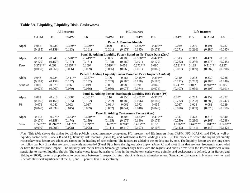
of insurance companies. In Table 3A, we attempt to add the respective factors to our analysis by

constructing new factors that capture those variables. Just like what Fama and French (2015) did

in the case of SMB, HML, RMW, and CMA and following the literature (see below), we form these

factors as long-short portfolios that buy/short top/bottom quintile from the sorts of all firms in the

market on the characteristic in question.5

For liquidity, we use two characteristics: Zero, the fraction of no-trade (zero return, zero

trading volume) days, which is a catch-all trading cost measure suggested by Lesmond et al.

(1999), and Amihud, the price impact measure from Amihud (2002). Lesmond et al. argued that

firms with higher trading costs will see more days when investors perceive the costs of trading to

be higher than benefits and refrain from trading. Amihud suggested averaging the ratio of absolute

value of return to dollar trading volume over a month or a year (we use a year) to gauge by how

much, on average, a trade of a given size (say, $1 million) moves the prices against the person

trading (a large buy order, for example, makes prices increase and the buyer has to pay a higher

price as a result).

The first panel of Table 3A reports the alphas of all insurers and two subgroups of P/L and

life insurers for the baseline models (CAPM, FF5, ICAPM, and FF6), effectively collecting this

5 The returns of all firms used for forming the liquidity factors, as well as trading volume data needed to compute the liquidity measures, are from CRSP.

6

information from Table 2 in the paper and Table 1A. The alphas are important, because the change

in them, once we start adding more factors, will be the gauge of the economic importance of these

factors. Any asset-pricing model partitions in-sample average return into the alpha (abnormal

return) and the rest (expected return or cost of equity). Since the average return is the same (as

long as the sample does not change), the change in the alpha has to equal the negative of the change

in expected return.

Panel B of Table 3A adds the liquidity factor based on the no-trade measure (Zero) into the

four models after which the columns are named and reports the alpha and the loading on the

liquidity factor (all other betas are not reported for brevity). Panel B reveals three main results.

First, in all models all groups of insurers load positively on the liquidity factor, suggesting that

insurance companies are likely to be among the firms the factor buys (illiquid firms). Second, the

liquidity factor is largely subsumed by SMB, HML, RMW, and CMA: as one goes from

CAPM/ICAPM to FF5/FF6, the liquidity factor beta shrinks in 3-5 times and generally loses

significance. Third, consistent with the above, adding the liquidity factor to CAPM/ICAPM

changes the alpha (and hence, COE estimates) by economically sizeable 10-20 bp per month (1.2-

2.4% per year), but adding it to FF5/FF6 changes the alpha and COE by at most 3 bp per month,

which is economically small.

Panel C replaces the Zero liquidity factor by Amihud liquidity factor and finds even weaker

results. The Amihud factor is rarely significant, the signs of the loadings alternate in different

models, and even when the Amihud factor is significant (CAPM/ICAPM for life insurers),

controlling for SMB, HML, RMW, and CMA effectively reduces it to zero. Consequently, the

difference between alphas in Panels A and C is just a few bps, suggesting that controlling for the

Amihud factor does not materially change COE estimates for insurance companies.

7

Summing up the evidence in Panels B and C, we conclude that liquidity has limited

explanatory power for insurers’ cost of equity, especially after we control for SMB, HML, RMW,

and CMA, which are part of one of our benchmark models (FF5). Thus, we do not feel the need to

further include liquidity factors in our analysis.

Panel D studies liquidity risk, which is a different concept. While liquidity refers to costs

of trading that have to be compensated in the before-cost returns (i.e., the returns all asset-pricing

literature uses), liquidity risk is a risk in the ICAPM sense and refers to losses during periods of

market illiquidity. In their influential paper, Pastor and Stambaugh (2003) suggest their own price

impact measure, compute it for each firm-month, and then average across all firms in each month.

This series of monthly market-wide average of price impact is their liquidity measure, and the

shocks to this series are liquidity shocks (constructed so that a positive shock means an increase

in liquidity).

Panel D uses the Pastor-Stambaugh factor (PS), which is the return differential between

firms with highest and lowest historical liquidity betas (high liquidity beta implies steep losses in

response to liquidity decreases, i.e., liquidity risk). 6 Panel D reveals that while the factor loadings

of insurance firms on the PS factor are uniformly negative (suggesting that insurers are hedges

against liquidity risk), these loadings are insignificant, and controlling for the PS factor has little

influence on alphas and hence on the cost of equity estimates.

Panel E looks at the role of skewness, which is known to be high in insurers’ returns due

to catastrophic losses. When it comes to measuring systematic risk though, the correct variable to

look at is coskewness (covariance of stock returns of a portfolio with squared market returns),

6 The values of the Pastor-Stambaugh factor are periodically updated by its creators and are available through WRDS to all subscribers.

8

because it measures the contribution of the asset to the skewness of a well-diversified portfolio.7

We measure coskewness betas for each firm-month using the formula in Harvey and Siddique

(2000):

𝛽𝛽𝑆𝑆𝑆𝑆𝑆𝑆𝑆𝑆 = 𝐸𝐸(𝜖𝜖𝑖𝑖𝑖𝑖 ∙ 𝜖𝜖𝑀𝑀𝑖𝑖2 )

�𝐸𝐸�𝜖𝜖𝑖𝑖𝑖𝑖2 � ∙ 𝐸𝐸(𝜖𝜖𝑀𝑀𝑖𝑖

2 ) (1)

where 𝜖𝜖𝑖𝑖𝑖𝑖 = 𝑅𝑅𝑖𝑖𝑖𝑖 − 𝑅𝑅𝑅𝑅𝑖𝑖 − 𝛼𝛼 − 𝛽𝛽 ∙ (𝑅𝑅𝑅𝑅𝑖𝑖 − 𝑅𝑅𝑅𝑅𝑖𝑖), and 𝜖𝜖𝑀𝑀𝑖𝑖 is the deviation of the market return from

the long-run average. To form our coskewness factor (Skew), we sort all firms in the market on the

historical coskewness betas and go long/short in the top/bottom quintile.

Panel E reveals that insurance companies have positive and significant exposure to the

coskewness factor, indicating their exposure to the risk picked up by coskewness. However, the

loading on the coskewness factor drastically decreases once we control for SMB, HML, RMW,

CMA, and FVIX. Further, the alphas of FF6 in Panel A and the seven-factor model of FF6 plus

Skew in Panel E differ by 1.5-5 bp per month, suggesting that the coskewness factor is

economically insignificant once the other market-wide factors are controlled for.

Appendix C: Cross-Sectional Tests and GRS Tests of the Models

Cross-Sectional Test of the Models Used in the Paper

In this part we perform the cross-sectional test of the four main models (CAPM, FF5,

CCAPM, and ICAPM) using industry portfolios as our cross-section. Table 4A presents the

estimates from the second stage regression of returns on past betas and reports Fama-MacBeth

(1973) t-statistics. The test follows the standard procedure: we first estimate the average betas

(market beta, FVIX beta, etc.) for each industry portfolio formed as in Fama and French (1997)

7 The standard CAPM uses a very similar logic: the non-systematic risk of an asset is the variance of the asset’s returns, but the systematic risk of the asset is measured by the market beta, which is proportional to covariance between the asset’s return and the market return, because the covariance measures the contribution of the asset to the variance of a diversified portfolio.

9

and then regress t+1 returns to the 30 industry portfolios on time t estimates of the betas. The time

t betas are estimated individually for each firm in the industry portfolio using t-59 to t returns (at

least 36 valid observations are required); the estimates are then trimmed at 1% and 99% in each

month and averaged within each industry portfolio.

The main finding from Table 4A is that all the models except for ICAPM do not do a good

job in the cross-section in our sample period (1986-2014, determined by the availability of FVIX).

Our tests lack power to state that any of the betas (including market beta, SMB beta, HML beta,

RMW beta, and CMA beta) are priced. FVIX is a fortunate exception with a t-statistic of -2.16. The

scaled factors from CCAPM (DEFt-1*(RM-RF), DIVt-1*(RM-RF), and TERMt-1*(RM-RF)) come

close to 10% significance, but are not there. Therefore, we do not implement the standard errors

corrections from Kan, Robotti, and Shanken (2013) – these corrections account for the estimation

error and model misspecification error and always make the t-statistics smaller, and we already do

not have any significant numbers in Table 4A, including the Fama-French five factor betas. In

other words, using Kan, Robotti, and Shanken (2013) corrections will only exacerbate the

conclusion that none of the factors in these tested models (except for FVIX) explain the cross-

section of industry returns.

The insignificance of most factors in cross-sectional tests is a common problem that

plagues those tests (see the results of testing many competing models in Kan, Robotti, and

Shanken, 2013, and Lewellen, Nagel, and Shanken, 2010) and makes many asset-pricing papers

starting with Fama and French (1993) revert to time-series regressions and alphas on the suspicion

that cross-sectional regressions simply lack power to reject the null that an important factor is not

priced. We also go this route in the paper.

Lewellen, Nagel, and Shanken (2010) suggest that asset pricing models should be

evaluated on two “common sense” metrics. First, the risk premiums estimated from the second-

10

stage regressions such as the ones in Table 4A have to be equal to the average risk premiums to

the factors we observe in the sample. For example (and this is where almost all models fail), the

slope on the market beta in the cross-sectional regression should be equal to the market risk

premium (the difference between the average market return and the average risk-free rate). In

1986-2014, the average market risk premium is 0.656% per month (roughly 8% APR). This is

somewhat high by historical standards and is probably driven by the sharp run-up in the market

during the 1990s.

Second, Lewellen, Nagel, and Shanken (2010) suggest paying a close attention to the

intercept. By definition, the intercept is the expected return to an asset with all betas equal to zero,

that is, the risk-free rate. In our sample, the risk-free rate is 0.29% per month (roughly 3.5% APR).

This is somewhat low by historical standards and is probably driven by the zero interest rates in

2008-2014.

If a model estimates, for example, the risk-free rate to be 15% APR and the market risk

premium to be 1%, this model is bad no matter what the R-squared is, because such a model just

does not make sense. In Table 4A this is what happens to both the CAPM and the FF5 model. Both

estimate the risk-free rate at roughly 10% APR and the market risk premium is estimated to be at

least twice smaller than it really is.

The ICAPM in the fourth column produces the most realistic estimates. While the risk-free

rate is still too high, the observed average risk-free rate is now within the confidence interval, and

the market risk premium estimate (0.717% per month) is almost exactly equal to its in-sample

average (0.656% per month). The risk premium of FVIX estimated from the cross-sectional

regression (-1.166% per month) is also close to the average FVIX return (-1.342% per month). The

CCAPM in the third column produces an even more realistic estimate of the risk-free rate, but the

market risk premium is too low (similar to FF5). Hence, on this “common sense” metric (realistic

11

estimates of the market risk premium and the risk-free rate) the models rank as ICAPM, then

CCAPM, then FF5, and then CAPM.

If one orders the models by the cross-sectional R-squared in the last row, the CCAPM

comes out on top, followed by the FF5 model and the ICAPM. We do not believe, however, that

R-squared is a good measure to compare the models on. First, as Lewellen, Nagel, and Shanken

(2010) argue, if the model produces obviously biased estimates of the risk-free rate and risk

premiums, it is a bad model regardless of the goodness of fit. Second, all asset-pricing tests mean

to analyze the drivers of expected return, but use realized returns instead, since expected return is

unobservable. Realized return is expected return plus the news component (in the case of the

industry portfolios Table 4A is looking at, it is industry news). So, the model will not have a perfect

fit even if it is 100% correct, because a perfect fit (R-squared =100%) is equivalent to industry

news being non-existent (which is obviously false) or risk factors completely capturing them

(which should not happen if the factors are truly economy-wide). Third, another reason why cross-

sectional R-squared might be inappropriate to compare models is due to what Lewellen, Nagel,

and Shanken (2010) discuss as “factor structure” – the returns to size-sorted portfolios, for

example, can be very well explained, in terms of R-squared, by a size factor or something even

remotely correlated with it. Likewise, if HML (or any other factor) is tilted towards a certain

industry, its betas will be explaining the cross-section of realized returns to industry portfolios

“better” in terms of R-squared due to their ability to pick up the industry-specific shocks to the

industry/industries that the factor is tilted towards. (Again, this problem would not exist if we could

observe expected returns and regress them on the factors/factor betas, but we can only observe

realized returns).

In terms of the problem at hand (cost of equity estimation), we are also interested in

expected returns (same thing as COE) and not that interested in the ability of the factors/factor

12

betas to pick up industry-specific shocks. If these shocks are random and zero-mean, tracking them

will increase the R-squared, but will not increase the expected return/COE estimate. Hence, we are

interested mostly in the intercept in the second-stage regressions in Table 4A and in the intercept

(aka alpha) from the first-stage factor regressions like the ones we report in the paper (Table 2 for

example).

GRS test of the Models Used in the Paper

To make sure that the results in Panels B and C of Table 1 in the paper are not specific to

the industry portfolios, we repeat the test suggested by Gibbons, Ross, and Shanken (1989), known

as the GRS test in the asset-pricing literature, for several other salient portfolio sets. In particular,

we look at five-by-five double sorts on size and market-to-book, five-by-five sorts on size and

momentum (momentum is one of the most well-known anomalies; the momentum factor is used

in another popular benchmark model originating from Carhart, 1997), and five-by-five sorts on

size and long-term reversal, as well as five-by-five sorts on size and profitability and size and

investment (profitability and investment are the two new factors in the five-factor model by Fama

and French, 2015).8

Table 5A presents the test of the hypothesis that the alphas of the 25 portfolios (named in

the panel heading) are jointly zero in the models named in the top row of each panel (failure to

reject the null indicates the model is a good one based on GRS test). Since the portfolios represent

important anomalies that have defied explanation, all models are rejected in almost all cases (the

only exception is Panel C, in which FF5, ICAPM and CCAPM, but not CAPM and FF3, seem to

explain the alphas of size-reversal sorts relatively well).

8 All portfolio returns are from Ken French’s data library at http://mba.tuck.dartmouth.edu/pages/faculty/ken.french/data_library.html.

http://mba.tuck.dartmouth.edu/pages/faculty/ken.french/data_library.html

13

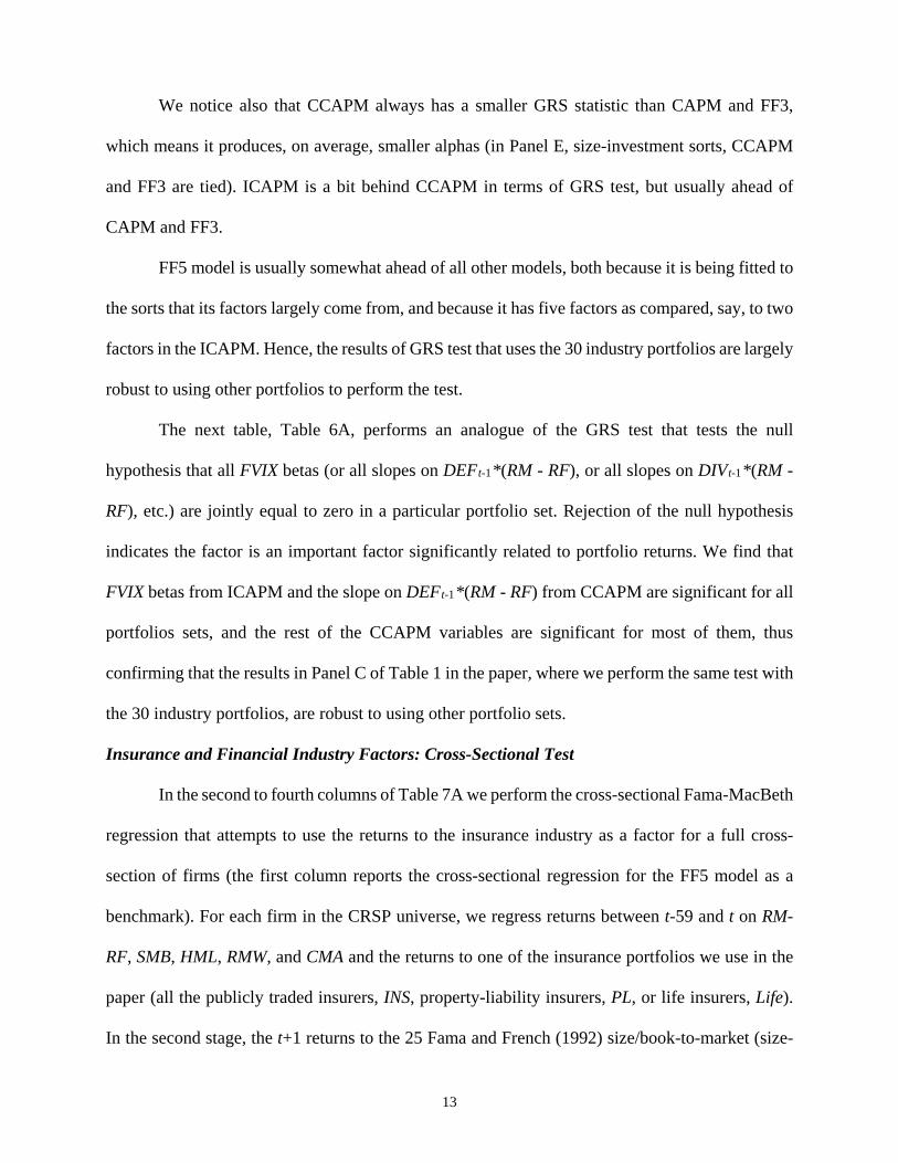
We notice also that CCAPM always has a smaller GRS statistic than CAPM and FF3,

which means it produces, on average, smaller alphas (in Panel E, size-investment sorts, CCAPM

and FF3 are tied). ICAPM is a bit behind CCAPM in terms of GRS test, but usually ahead of

CAPM and FF3.

FF5 model is usually somewhat ahead of all other models, both because it is being fitted to

the sorts that its factors largely come from, and because it has five factors as compared, say, to two

factors in the ICAPM. Hence, the results of GRS test that uses the 30 industry portfolios are largely

robust to using other portfolios to perform the test.

The next table, Table 6A, performs an analogue of the GRS test that tests the null

hypothesis that all FVIX betas (or all slopes on DEFt-1*(RM - RF), or all slopes on DIVt-1*(RM -

RF), etc.) are jointly equal to zero in a particular portfolio set. Rejection of the null hypothesis

indicates the factor is an important factor significantly related to portfolio returns. We find that

FVIX betas from ICAPM and the slope on DEFt-1*(RM - RF) from CCAPM are significant for all

portfolios sets, and the rest of the CCAPM variables are significant for most of them, thus

confirming that the results in Panel C of Table 1 in the paper, where we perform the same test with

the 30 industry portfolios, are robust to using other portfolio sets.

Insurance and Financial Industry Factors: Cross-Sectional Test

In the second to fourth columns of Table 7A we perform the cross-sectional Fama-MacBeth

regression that attempts to use the returns to the insurance industry as a factor for a full cross-

section of firms (the first column reports the cross-sectional regression for the FF5 model as a

benchmark). For each firm in the CRSP universe, we regress returns between t-59 and t on RM-

RF, SMB, HML, RMW, and CMA and the returns to one of the insurance portfolios we use in the

paper (all the publicly traded insurers, INS, property-liability insurers, PL, or life insurers, Life).

In the second stage, the t+1 returns to the 25 Fama and French (1992) size/book-to-market (size-

14

BM) portfolios (Panel A) or the 30 Fama and French (1997) industry portfolios (Panel B), are

regressed, in cross-section, on time t estimates of the betas from t-59 to t, as described above.

The main result in Panel A is that adding the insurance factors does not change much either

in terms of the intercept (the risk-free rate is still being estimated at unreasonably high values that

exceed 1% per month), or the market risk premium, or the R-squared. Also, none of the insurance

factor betas are statistically significant and their estimated risk premiums controlling for the Fama-

French five factors are small (just like their small Fama-French alphas in Table 2 (FF5 column) in

the paper).

The two rightmost columns add the Adrian et al. (2016) financial industry factors instead

of the insurance factors: first, to the three-factor Fama-French model, as Adrian et al. (2016) do

(AFM column), and then to the FF5 model (FF5+AFM column). The only marginally significant

beta is the FROE beta in the AFM model, but it has the wrong sign, because, first by construction,

the average return to FROE is positive, and, second, the slope on the beta in cross-sectional

regressions should equal the risk premium earned by the factor, so in our case if the AFM model

had had a good fit, the slope on the FROE beta should have been positive. The intercepts of the

AFM and FF5+AFM models are also very close to the intercept of the FF5 model, implying that

FROE and SPREAD do not improve the goodness of fit of the models. The increases in the R-

squared we observe comparing the AFM and FF5+AFM models with the FF5 model are likely to

be driven by the wrong sign of FROE beta.

In Panel B, we redid the analysis again with the 30 industry portfolios. The results are very

similar and even worse for the insurance factors: their risk premiums are now estimated to be much

lower, and the risk premium of the Life factor flips its sign. All other factors (RM-RF, SMB, HML,

RMW, and CMA) still lack significance, and the same is true about FROE and SPREAD. The AFM

model is very close to the FF5 model in terms of R-squared, and the FF5+AFM model has a better

15

R-squared, but worse (larger) intercept, which represents an unrealistically high estimate of the

risk-free rate (0.815% per month, roughly 10% per year in the case of the FF5+AFM model).

Since the Fama-French factors are insignificant, we also tried dropping (some of) them and

adding the insurance factors or AFM factors to the CAPM/FF3 (results not tabulated). In general,

that would bias the test in favor of finding that the insurance factors matter – any diversified

portfolio that is significantly correlated with either of the four Fama-French factors (SMB, HML,

RMW, and CMA) (and, according to Table 2 in the paper, our insurance factors have significant

SMB, HML, and RMW betas) can act as their proxy and seem to matter in addition to the market

factor even if it has no additional information compared to SMB, HML, or RMW and thus is not

priced controlling for those factors. However, Table 7A suggests that the four Fama-French factors

are themselves not priced in our sample period, so the overlap between them and the insurance

factors is less of a concern. Indeed, when we add the insurance factors to the CAPM, we find that

they still do not price the five-by-five size-BM sorts or the 30 industry portfolios. None of the

insurance/AFM factors is significant and what is even worse, the intercept (that estimates the risk-

free/zero-beta rate) becomes noticeably larger and goes further into the implausible territory when

we add the insurance/AFM factors to the CAPM/FF3.

We also tried extending the sample to 1963 to run the analyses in both Panels A and B in

Table 7A (the start of Compustat data) to gain more power. We did achieve significance for the

HML beta and marginal significance (along with a positive coefficient) for the SMB beta, but the

betas of the insurance/AFM factors are still insignificant even in the longer sample, often negative,

and adding them has a small effect on the R-squared and makes the intercept somewhat greater

(that is, makes the overestimation of the risk-free rate slightly worse).

Insurance and Financial Industry Factors: GRS Test

16

Columns 2-4 of Table 8A test for the joint insignificance of alphas from time-series

regressions with insurance factors on the left-hand side using the GRS test (column 1 of Table 8A

performs the GRS test for the FF5 model as a benchmark). The point of Table 8A is the comparison

of the FF5 model (first column) with the FF5 model augmented, in turn, by each of the insurance

factors, as well as with the AFM and FF5+AFM models.

One can see from Panel A of Table 8A that adding the insurance factors does not change

the test statistic in a material way, which implies that the effect of adding either of the insurance

factors on the alphas of the 25 size-BM sorted portfolios is minimal and insurance factors are

effectively not priced. This is not surprising, since, as we show in Table 2 in the paper, none of the

insurance portfolios (all the publicly traded insurers, P/L insurers, or life insurers), now used as

factors, have a significant alpha in the FF5 model. Hence, controlling for RM-RF, SMB, HML,

RMW, and CMA, the risk premium of the insurance factors is essentially zero, and no matter

whether some portfolios in the size-BM sorts load significantly on them or not, adding the

insurance factors should not change the alphas of these size-BM portfolios (and it does not, as

evidenced in Panel A of Table 8A).

In the subsequent panels of Table 8A, we also repeat the GRS test for the FF5 model and

the FF5 model augmented with the insurance factors using four more portfolio sets, which are five-

by-five sorts on size and other salient variables (momentum, long-term reversal, profitability, or

investment). For all portfolio sets in the four panels B-E, adding the insurance factors either makes

the GRS test statistics bigger, indicating that the insurance factors make the model fit worse, not

better (size-momentum and size-reversal sorts) or does not affect the GRS test statistic at all,

indicating that the insurance factors are useless (size-investment sorts).

Finally, in the two rightmost columns of each panel, we perform the GRS test for the AFM

and FF5+AFM models. We observe that the AFM model is behind the FF5 model in terms of the

17

GRS test statistic (which implies that the AFM model has larger pricing errors) and the FF5+AFM

model generates GRS test statistics that are very close to the ones from FF5 (or FF5 augmented

with an insurance factor). We conclude that the two financial industry factors suggested in Adrian

et al. (2016), FROE and SPREAD, are close in their performance to the insurance factors – they

do not add much to the explanatory power of the FF5 model and are largely unpriced.

Overall, our conclusion from both the cross-sectional Fama-MacBeth regressions and the

time-series GRS tests is that the insurance and financial industry factors do not contribute to

explaining the cross-section of returns in a material way, because they are industry-specific factors

that can be diversified away if an investor invests in multiple industries. This is also consistent

with related evidence in the paper (Tables 4-6), where we consider other potential insurance-

industry-specific factors.

Appendix D: Other Types of Insurers

The insurance industry includes other types of companies with arguably very different risks

and operating characteristics from the P/L and life insurance companies. In this section, we apply

the same tests in Tables 2 and 3 in the paper to the other types of insurers and investigate whether

the results are consistent with the P/L and life insurers that are usually considered to represent the

insurance industry. Since the monthly average numbers of surety insurers, title insurers, pension,

health, welfare funds, and other insurance carriers are very small (low teens for surety insurers and

single digits for others), we put these insurers together as a combined category (other insurers).9

Therefore we divide the insurance industry into four major groups, namely, property-liability (P/L)

9 The insurance industry is classified into seven categories, namely, life insurance (SIC 6310-6319), accident and health insurance (SIC 6320-6329), property-liability insurance (SIC 6330-6331), surety insurance (SIC 6350-6351), title insurance (SIC 6360-6361), pension, health, welfare funds (SIC 6370-6379), and other insurance carriers (SIC within 6300-6399 but do not fall into any of the previous six categories).

18

insurers (SIC codes 6330-6331), life insurers (6310-6311), accident and health (A/H) insurers

(6320-6329), and other insurers (all other firms with 6300-6399).

We run the four asset pricing models (CAPM, FF5, CCAPM, and ICAPM as shown in

Table 2 in the paper) as well as the AFM model (in Table 1A) on A/H insurers and other insurers

in addition to all insurers, P/L insurers, and life insurers. The additional results are reported in

Table 9A.

The results in Table 9A are consistent with the results of all, P/L, and life insurers reported

in Table 2 in the paper and Table 1A. The CCAPM regression results in Panel A indicate that the

beta of A/H insurers significantly increases with the dividend yield (DIV), and significantly

decreases with the Treasury bill rate (TB) and term premium (TERM). Since dividend yield is

higher and Treasury bill rate is lower in recessions, the significant coefficients on DIV and TB

indicate that the beta of A/H insurance companies is countercyclical, which makes them riskier

than what the CAPM would suggest. However, the significantly negative coefficient on TERM

indicates that A/H insurers may have procyclical beta, since term premium is higher in recessions.

When confronted with such conflicting evidence, we can compare the alpha in the CAPM and

CCAPM column. We observe that it decreases by economically non-negligible 14.4 bp per month

(1.73% per year) as we go from the CAPM to CCAPM. Hence, the CCAPM discovers more risk

in insurance companies than CAPM, and for that to be true, the beta of the insurance companies

has to be countercyclical (representing additional risk). Furthermore, a formal test of

countercyclical or procyclical beta is performed in Panels C and D of Table 9A.

In Panel B, dividend yield and Treasury bill rate stay as the significant drivers of the risk

of other insurers, and the signs suggest the countercyclicality of beta; DEF and TERM are

insignificant, but the signs also indicate the countercyclicality of other insurers’ beta.

19

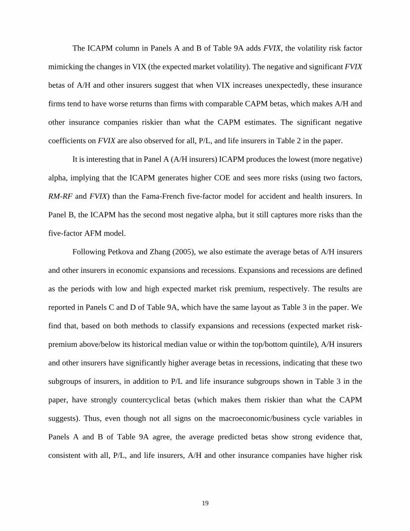
The ICAPM column in Panels A and B of Table 9A adds FVIX, the volatility risk factor

mimicking the changes in VIX (the expected market volatility). The negative and significant FVIX

betas of A/H and other insurers suggest that when VIX increases unexpectedly, these insurance

firms tend to have worse returns than firms with comparable CAPM betas, which makes A/H and

other insurance companies riskier than what the CAPM estimates. The significant negative

coefficients on FVIX are also observed for all, P/L, and life insurers in Table 2 in the paper.

It is interesting that in Panel A (A/H insurers) ICAPM produces the lowest (more negative)

alpha, implying that the ICAPM generates higher COE and sees more risks (using two factors,

RM-RF and FVIX) than the Fama-French five-factor model for accident and health insurers. In

Panel B, the ICAPM has the second most negative alpha, but it still captures more risks than the

five-factor AFM model.

Following Petkova and Zhang (2005), we also estimate the average betas of A/H insurers

and other insurers in economic expansions and recessions. Expansions and recessions are defined

as the periods with low and high expected market risk premium, respectively. The results are

reported in Panels C and D of Table 9A, which have the same layout as Table 3 in the paper. We

find that, based on both methods to classify expansions and recessions (expected market risk-

premium above/below its historical median value or within the top/bottom quintile), A/H insurers

and other insurers have significantly higher average betas in recessions, indicating that these two

subgroups of insurers, in addition to P/L and life insurance subgroups shown in Table 3 in the

paper, have strongly countercyclical betas (which makes them riskier than what the CAPM

suggests). Thus, even though not all signs on the macroeconomic/business cycle variables in

Panels A and B of Table 9A agree, the average predicted betas show strong evidence that,

consistent with all, P/L, and life insurers, A/H and other insurance companies have higher risk

20

exposure in bad times, which is undesirable from investors’ point of view and leads investors to

demand higher cost of equity.

Appendix E: FVIX Exposures of 48 Fama-French (1997) Industry Portfolios

The question of how the other industries do in terms of volatility risk exposure, is an

interesting one. In Table 10A we investigate the 48 industry portfolios from Fama and French

(1997). The portfolios span the whole economy and include insurance and related industries (the

bottom panel). We find that while negative FVIX betas dominate our sample (higher volatility is

generally bad for everyone), roughly a third of FVIX betas are positive, and the average FVIX beta

across all 48 industries is only -0.141 (compared to -0.866 for the insurance industry). We also

notice that the FVIX beta of the insurance industry is the 5th most negative (behind Food, Soda,

Beer, and Smoke in the top panel). Hence, the insurance industry does differ from an average

industry.

Appendix F: More Details on Underwriting Cycles and the Intertemporal CAPM

In addition to the average combined ratio documented in Section V of the paper, we have

experimented with another insurance-specific variable—total catastrophic losses to create the

ICAPM factor. In this section, we demonstrate the results of the factor-mimicking regressions for

both candidate insurance-specific variables (cat losses and the combined ratio) on the base assets,

analyze the alphas and betas of the factor-mimicking portfolios in the CAPM, FF3, Carhart (1997),

and FF5 models, and explore the regressions that try to add the factor-mimicking portfolio for

inflation-adjusted catastrophic losses (in addition to change in combined ratio in Table 6 in the

21

paper) to the models (CAPM, ICAPM, FF5, and FF5 augmented with FVIX (FF6)) we use in the

paper.

Table 11A presents the results of factor-mimicking regressions on the base assets. The

factor-mimicking regressions attempt to create a tradable portfolio that would correlate well with

shocks to total catastrophic losses or average combined ratio. Since catastrophic losses are largely

unpredictable and their autocorrelation is low, we treat the values of catastrophic losses as shocks.

For combined ratio, a much more persistent variable with autocorrelation close to 1, we use its

changes as a proxy for shocks.

Lamont (2001) suggests that the optimal base assets should have the richest possible

variation in the sensitivity with respect to the variable being mimicked. Therefore, we choose

quintiles based on historical sensitivity to catastrophic losses or change in combined ratio. In each

firm-quarter (insurance-specific/underwriting cycle variables such as catastrophic losses and

combined ratio are collected quarterly) for every stock traded in the US market and listed on CRSP,

we perform regressions of excess stock returns on RM-RF, SMB, HML, and either inflation-

adjusted catastrophic losses (CatLoss) or change in combined ratio (ΔCombRat). The slope on

CatLoss or ΔCombRat is our measure of historical stock sensitivity to catastrophic losses or change

in combined ratio.

The regressions use quarterly returns and the most recent 20 quarters of data (that is, in

quarter t we use data from quarters t-1 to t-20) and omit stocks with less than 12 non-missing

returns between t-1 and t-20.

To obtain the base assets for mimicking catastrophic losses or change in combined ratio,

we sort all firms on CRSP on the historical stock sensitivity to catastrophic losses or change in

combined ratio in five quintile portfolios. To minimize the impact of micro-cap stocks, we use

NYSE breakpoints to form the quintiles and omit from the sample stocks those priced below $5 at

22

the quintile formation date. Table 11A performs the standard factor mimicking regression with

CatLoss (columns 1 and 2) or CombRat (columns 3 and 4) on the left-hand side and excess returns

to value-weighted and equal-weighted quintile portfolios based on the historical stock sensitivity

to catastrophic losses and change in combined ratio on the right-hand side, respectively.10

Table 11A shows that creating the factor-mimicking portfolio for either variable has

limited success, because total catastrophic losses and shocks to average combined ratio seem to be

unrelated to returns of any of the historical sensitivity quintiles. That is to say, when the insurance

industry suffers a shock, the rest of the economy seems largely unaffected, consistent with similar

findings in Table 4 of the paper that insurance-specific variables that drive the underwriting cycles

do not predict the market risk premium. Consequently, the R-squared of the factor-mimicking

regressions is only a few percent.11

Tables 12A and 13A look at the alphas and betas of the factor-mimicking portfolios

constructed in Table 11A in the CAPM, FF3, Carhart, and FF5 models. The factor-mimicking

portfolios are the fitted part from the regressions in Table 11A less the constant. The factor-

mimicking regressions in Table 11A are performed at the quarterly frequency, since this is the

frequency at which total catastrophic losses and average combined ratio are reported. However,

the factor-mimicking portfolio returns are monthly, because returns to the base assets (stock sorted

on historical stock sensitivity to catastrophic losses or change in combined ratio) are also available

at the monthly frequency, and the factor-mimicking portfolio just multiplies them by the slopes

from Table 11A.

10 Column 3 effectively contains the equation for the combined ratio factor, FCombRat, used in Table 6 in the paper. 11 In untabulated results, we also experimented with using different quintile breakpoints for the quintiles sorted on the historical stock sensitivity to catastrophic losses or change in combined ratio, or replacing these quintiles with two-by-three sorts on size and book-to-market from Fama and French (1993). The results in Tables 11A-14A and Table 6 in the paper are qualitatively the same when we do that.

23

We observe, first of all, that the alphas uniformly have the correct negative sign (the

portfolios are constructed so that they win when total catastrophic losses or average combined ratio

increases and insurance companies lose, and thus can be regarded as a hedge). However, the alphas

are economically negligible (less than 1 bp per month) and mostly statistically insignificant for the

factor-mimicking portfolio for CatLoss (see Table 12A); the alphas are economically small (1-3

bp per month on average) and all statistically insignificant for the factor-mimicking portfolio for

ΔCombRat (see Table 13A). We conclude that investors are not willing to give up a significant

return for a hedge against potential problems in the insurance industry, allegedly because the

insurance industry losses do not impact the economy as a whole and the vast majority of investors

are not materially affected by them, and also because the industry-specific risks can be diversified

away.

The observation that the alphas of the factor-mimicking portfolios that track shocks to

insurance-industry-specific variables are small is an important one. The alpha measures the unique

risk captured by the factor (controlling for the other factors used in the alpha estimation). In terms

of cost of capital, the alpha is the potential marginal contribution of the factor. Low-alpha factors

(such as the factor-mimicking portfolios on catastrophic losses and changes in combined ratio in

Tables 12A and 13A) have little chance to contribute materially to the cost of capital estimates if

added into a factor model.

The betas of the factor-mimicking portfolios in Tables 12A and 13A are surprisingly

significant, but numerically small. While the significance creates an (allegedly misleading)

impression that shocks to the insurance variables are related to market-wide factors (RM-RF, SMB,

HML, and sometimes CMA and RMW), the relation is economically negligible.

Table 14A contains regressions that try to add the value-weighted factor-mimicking

portfolio for inflation-adjusted catastrophic losses (FCatLoss) to the models we use in the paper

24

(CAPM, ICAPM, FF5, and FF6) and thus repeats Table 6 in the paper replacing the factor that

mimics combined ratio with the factor mimicking catastrophic losses. The results of estimating the

models used in the paper are in columns 1, 4, 7, and 10. The factor is added to the models in

columns 2, 5, 8, and 11. In columns 3, 6, 9, and 12 the factor is replaced by the variable the factor

mimics (catastrophic losses, CatLoss). The left-hand side variable is the value-weighted returns to

all publicly traded insurance companies. Changing it to equal-weighted returns or dividing the

sample into P/L insurers and life insurers does not materially change the results.12

Similar to the results reported in Table 6 in the paper when adding the factor-mimicking

portfolio for changes in combined ratio, in columns 8 and 11 of Table 14A we observe that the

betas of all insurance companies with respect to the FCatLoss factor lose significance after we

control for the factors our main analysis uses (RM-RF, SMB, HML, CMA, and RMW, or these

factors plus FVIX). We checked (columns 9 and 12 of Table 14A) that the insignificant betas are

not an artefact of our factor-mimicking procedure by replacing the factor-mimicking portfolio with

catastrophic losses, which still produces insignificant loadings. In addition, we observe that the

impact on the alphas of adding FCatLoss to models other than CAPM (namely, ICAPM, FF5, and

FF5+FVIX) is minor, consistent with our findings regarding changes in combined ratio in Table 6

in the paper. In conclusion, adding the insurance industry factor-mimicking portfolios as

insurance-specific factors does not change estimated cost of equity. The economic reason is that

shocks specific to the insurance industry do not affect the economy as a whole and can be

diversified away by investors who invest in many industries. Therefore, these shocks do not

represent priced risks and should not be expected to affect the cost of equity of insurance

companies (even if the shocks do affect their cash flows).

12 This statement holds true when adding the factor-mimicking portfolio on changes of combined ratio (ΔCombRat) to the models (CAPM, ICAPM, FF5, and FF6) based on Table 6 in the paper.

25

Appendix G: Cost of Equity Estimation from Augmented Fama-French and AFM Models

and from Sum-beta Approach

In addition to the cost of equity capital estimated based on the four main models (CAPM,

FF5, CCAPM, and ICAPM) in Table 7 in the paper, we estimate the value-weighted average COE

using the AFM model and Fama-French five-factor model augmented with FVIX (FF6) for each

of the 18 sample years (1997-2014) and 18 years combined. The results are presented in columns

5 and 6 in Table 15A in Panels A, B, and C for all publicly-traded insurance companies and the

two major subgroups (P/L insurers and life insurers), respectively. For comparison purposes, the

COE estimates from CAPM, FF5, CCAPM, and ICAPM are reported in columns 1-4 (same as

Table 7 in the paper).

We document that the COE estimates from the AFM model are higher than the CAPM

estimates, but they are lower than the FF5 estimates on average for all, P/L, and life insurance

companies. It suggests that the financial industry factors (FROE and SPREAD) do not reflect as

much risk as RMW and CMA for insurers. This is not surprising because the financial industry

factors, similar to the insurance factors, are industry-specific factors that can be diversified away

if the marginal financial portfolio investor also invests in many other industries. As a matter of

fact, in untabulated results, we show that FROE has insignificant alpha controlling for FF5 factors

and SPREAD’s alpha even has the “wrong” sign (implying that higher SPREAD beta means low

expected return/COE, but by construction of SPREAD it should be the opposite). It indicates that

adding the financial industry factors does not help in or even mislead (given the significant

SPREAD betas for various groups of insurers in Tables 1A and 9A) the cost of equity estimation

for insurance companies.

26

We find that the COE estimates from FF6 are even higher than those from FF5 on average

for all insurance companies and the two subgroups. It suggests that FVIX contributes to COE

estimation even controlling for SMB, HML, RMW, and CMA. Hence, it confirms the claim in

Appendix A that FVIX has independent explanatory power that goes beyond its overlap with RMW

and HML. The average COE for the 18-year period estimated from FF6 is 13.490%, 12.607%, and

15.688% per annum for all insurers, P/L insurers, and life insurers, respectively, as compared to

12.662%, 11.312%, and 15.366% per annum from FF5. For all insurance companies and the two

subgroups, ICAPM generates very similar COE estimates to those from FF6, indicating that

ICAPM finds about the same amount of risk in insurance companies during our sample period on

average as FF6. It confirms our conclusion in Appendix A that SMB, HML, RMW, and CMA do

not have much of explanatory power of their own for insurers beyond the overlap with FVIX.

Furthermore, following Cummins and Phillips (2005) we estimate the COE using the sum-

beta approach (Dimson, 1979) based on all the six models mentioned above (CAPM, FF5,

CCAPM, ICAPM, AFM, and FF6). The idea of Dimson is that for thinly traded stocks, the

information in the market return can be incorporated into stock prices with a delay, and thus one

should regress the stock returns on the market return from the same period t and also on the market

return from period t-1. The market beta is then the sum of the slopes on those two market returns.

For CAPM, FF5, ICAPM, AFM, and FF6, the estimated sum-beta coefficients are obtained

similarly by adding the slopes on the contemporaneous and lagged factor returns from these

models. Then the sum-beta COE is calculated by summing the products of the estimated sum-beta

coefficients multiplied by long-term factor risk premiums, plus the risk-free rate (more details on

the estimation window and factor risk premiums are in Estimation Methods subsection in Section

VI in the paper). For CCAPM the sum-beta COE is computed by summing the product of the

predicted contemporaneous beta with predicted contemporaneous market risk premium and the

27

product of the predicted lagged beta with predicted lagged market risk premium, plus current risk-

free rate. The sum-beta version of COE estimates is reported in columns 7-12 in Table 15A based

on different models for all insurance companies (Panel A), P/L insurers (Panel B), and life insurers

(Panel C). The presented COE estimates are value-weighted averages across all firms for each of

the 18 sample years (1997-2014) and 18 years combined.

The COE estimates based on the sum-beta approach are similar to those estimated without

the sum-beta approach. For all insurance companies and the P/L subgroup the difference between

the usual and sum-beta COE estimates is small across all models (generally under 1% per annum).

For life insurers, the difference is more material (over 3% for FF5, ICAPM, and FF6). Moreover,

we still find the ICAPM cost of equity estimates higher than those from the CAPM, AFM, and

FF5 models.

Appendix H: Equal-Weighted Returns of Insurers

We have been using value-weighted returns of insurance companies throughout the paper

and Online Appendices. As an additional robustness check, we replicated Tables 2, 3, 6, and 7 in

the paper using equal-weighted insurer returns and report them in Tables 16A, 17A, 18A, and 19A,

respectively.

Table 16A re-runs Table 2 in the paper using equal-weighted returns and fits several factor

models to all insurers, P/L insurers, and life insurers, respectively. We find the following. First,

the FVIX beta is still significant, though numerically smaller, for all insurers and P/L insurers, and

and insignificant (as compared to marginally significant at 10% in Table 2) for life insurers.

Second, the market beta of insurance companies is still countercyclical, positively related to

dividend yield (DIV) and negatively related to Treasury bill rate. For life insurers, a positive

dependence of the beta on default premium (DEF) and negative dependence on term premium

28

(TERM) are added. Third, the equal-weighted CCAPM and ICAPM alphas are again significantly

smaller than the CAPM alphas, implying that those models find additional sources of risk and will

generate higher cost of capital estimates, though in equal-weighted returns, in contrast to value-

weighted returns, the FF5 model sometimes generates even lower alphas (and finds even more

risk) than the ICAPM.

Table 17A repeats Table 3 in the paper using equal-weighted returns and tabulates the

market betas of the three groups of insurers (all, P/L, and life) in expansions and recessions. The

differences in the betas recessions vs. expansions (the ultimate proof of the insurers' betas

countercyclicality) are very close in Table 3 in the paper and Table 17A.

Table 18A repeats Table 6 and considers adding the change in combined ratio (ΔCombRat)

and its factor-mimicking portfolio (FCombRat) to the CAPM, FF5, ICAPM, and FF6 models. Both

ΔCombRat and FCombRat are still insignificant even when equal-weighted returns to all the

publicly traded insurers are used on the left-hand side, and adding them to the models does not

materially change the alphas or the FVIX betas.

We estimate the equal-weighted cost of equity for all, P/L, and life insurers and report the

results in Table 19A. The equal-weighted COE estimates are usually lower than the value-

weighted, but the difference is small with generally less than 1% on average across all models

except for those from the ICAPM. The equal-weighted ICAPM COE estimates are about 3% lower

than those value-weighted for all insurance companies and P/L insurers and 1.5% lower for life

insurers on average. The lower equal-weighted COE can be due to the following reasons. First, the

market betas across models are mostly lower in Table 16A (based on equal-weighted returns) than

in Table 2 in the paper (based on value-weighted returns). Second, even though the insurer equal-

weighted returns are higher than value-weighted returns (see Table 1 in the paper), the difference

is smaller than the difference between the equal-weighted and value-weighted alphas. As a result,

29

the equal-weighted COE estimates should turn out to be smaller than those value-weighted. Third,

according to Table 4 in Adrian et al. (2016) (the mean of) FSMB (the return differential between

the small financial and big financial firms) is less than zero, suggesting that the size effect is

negative for financial firms, and consequently, small financial firms have lower COE. Since equal-

weighted returns give more weights to small firms, the equal-weighted COE is lower. Further, for

the ICAPM specifically, comparing Table 16A and Table 2 in the paper, we find that the FVIX

betas are less than half in size using equal-weighted than value-weighted returns, indicating a lower

explanatory power for equal-weighted than value-weighted returns. However, the ICAPM

generates low COE estimates right before the Great Recession in 2008 and high estimates after it

(well reflecting the reality), while the other models do not. In sum, even though the ICAPM is

weaker when using equal-weighted insurer returns, our central message does not change: the

ICAPM produces higher COE estimates than the CAPM and the insurance companies are exposed

to the market volatility risk.

We also replicated all the other tables in the paper and most of the tables in Online

Appendices using insurer equal-weighted returns (results not tabulated to save space) and find that

the results with equal-weighted returns are qualitatively similar to the results with value-weighted

returns that we usually report.

References Adrian, T., E. Friedman, and T. Muir, 2016, The Cost of Capital of the Financial Sector, working paper, Federal

Reserve Bank of New York. Amihud, Y., 2002, Illiquidity and Stock Returns: Cross-Section and Time Series Effects, Journal of Financial

Markets, 5: 31-56. Barinov, A., 2011, Idiosyncratic Volatility, Growth Options, and the Cross-Section of Returns, working paper,

University of California, Riverside. Barinov, A., 2015, Profitability Anomaly and Aggregate Volatility Risk, working paper, University of California,

Riverside. Carhart, M.M., 1997, On Persistence in Mutual Fund Performance, Journal of Finance, 52: 57-82. Cummins, J.D., and R.D. Phillips, 2005, Estimating the Cost of Equity Capital for Property-Liability Insurers, Journal

30

of Risk and Insurance, 72: 441-478. Daniel, K., and S. Titman, 1997, Evidence on the Characteristics of Cross Sectional Variation in Stock Returns, The

Journal of Finance, 52: 1-33. Dimson, E., 1979, Risk Measurement when Shares are Subject to Infrequent Trading, Journal of Financial Economics,

7: 197-226. Fama, E.F., and K.R. French, 1992, The Cross-Section of Expected Stock Returns, Journal of Finance, 47: 427–465. Fama, E.F., and K.R. French, 1993, Common Risk Factors in the Returns on Stocks and Bonds, Journal of Financial

Economics, 33: 3–56. Fama, E.F., and K.R. French, 1995, Size and Book-to-Market Factors in Earnings and Returns, Journal of Finance,

50: 131-155. Fama, E.F., and K.R. French, 1996, Multifactor Explanations of Asset Pricing Anomalies, Journal of Finance, 51: 55-

84. Fama, E.F., and K.R. French, 1997, Industry Costs of Equity, Journal of Financial Economics, 43: 153-193. Fama, E.F., and K.R. French, 2002, The Equity Premium, Journal of Finance, 57: 637-659. Fama, E.F., and K.R. French, 2015, A Five-Factor Asset Pricing Model, Journal of Financial Economics, 116: 1-22. Fama, E.F., and J.D. Macbeth, 1973, Risk, Return and Equilibrium: Empirical Tests, Journal of Political Economy,

81: 607-636. Gibbons, M.R., S.A. Ross, and J. Shanken, 1989, A Test of the Efficiency of a Given Portfolio, Econometrica, 57:

1121-1152. Hahn, J., and H.Lee, 2006, Interpreting the Predictive Power of the Consumption-Wealth Ratio, Journal of Empirical

Finance, 13: 183-202. Harvey, C. R., and A. Siddique, 2000, Conditional Skewness in Asset Pricing Tests, Journal of Finance, 55: 1263-

1295. Jacoby, G., D. J. Fowler, and A. A. Gottesman, 2000, The Capital Asset Pricing Model and the Liquidity Effect: A

Theoretical Approach, Journal of Financial Markets, 3: 69-81. Kan, R., C. Robotti, and J. Shanken, 2013, Pricing Model Performance and the Two-Pass Cross-Sectional Regression

Methodology, Journal of Finance, 68: 2617-2649. Lakonishok, J., A. Shleifer, and R. Vishny, 1994, Contrarian Investment, Extrapolation, and Risk, Journal of Finance,

49: 1541-1578. Lamont, O.A., 2001, Economic Tracking Portfolios, Journal of Econometrics, 105: 161-184. Lesmond, D. A., J. Ogden, and C. Trzcinka, 1999, A New Estimate of Transaction Costs, Review of Financial Studies,

12: 1113-1141. Lewellen, J.W., S. Nagel, and J. Shanken, 2010, A Skeptical Appraisal of Asset Pricing Tests, Journal of Financial

Economics, 96: 175-194. Pastor, L. and R.F. Stambaugh, 2003, Liquidity Risk and Expected Stock Returns, Journal of Political Economy,

111: 642-685. Petkova, R., and L. Zhang, 2005, Is Value Riskier than Growth? Journal of Financial Economics, 78: 187-202. Wen, M., A.D. Martin, G. Lai, and T.J. O’Brien, 2008, Estimating the Cost of Equity for Property-Liability Insurance

Companies, Journal of Risk and Insurance, 75: 101-124.

31

Table 1A. Fama-French Five-Factor and AFM Models Augmented by Volatility Risk Factor

Panel A.

All Insurers Panel B.

P/L Insurers Panel C.

Life Insurers FF5 FF6 AFM AFM6 FF5 FF6 AFM AFM6 FF5 FF6 AFM AFM6

RM-RF 1.03*** 0.39** 0.89*** 0.45*** 0.90*** 0.03 0.75*** 0.13 1.35*** 1.43*** 1.24*** 1.62*** (0.04) (0.18) (0.03) (0.13) (0.04) (0.20) (0.03) (0.15) (0.06) (0.28) (0.05) (0.22)

SMB -0.13** -0.08 -0.08** -0.04 -0.29*** -0.22*** -0.22*** -0.16*** 0.06 0.05 0.15** 0.11 (0.06) (0.06) (0.04) (0.04) (0.06) (0.06) (0.05) (0.05) (0.08) (0.08) (0.07) (0.07)

HML 0.59*** 0.60*** 0.10* 0.09* 0.50*** 0.51*** 0.04 0.03 1.10*** 1.10*** 0.44*** 0.45*** (0.07) (0.07) (0.06) (0.05) (0.08) (0.08) (0.07) (0.06) (0.11) (0.11) (0.09) (0.09)

RMW 0.25*** 0.15* 0.20** 0.07 0.03 0.04 (0.08) (0.08) (0.09) (0.09) (0.11) (0.12) CMA -0.09 -0.14 -0.02 -0.08 -0.31** -0.30* (0.11) (0.11) (0.12) (0.12) (0.16) (0.16) FROE 0.05*** 0.04** 0.05** 0.04* 0.03 0.04 (0.02) (0.02) (0.02) (0.02) (0.03) (0.03) SPREAD 0.67*** 0.65*** 0.66*** 0.63*** 0.71*** 0.73*** (0.05) (0.05) (0.06) (0.05) (0.08) (0.08) FVIX -0.45*** -0.32*** -0.62*** -0.46*** 0.05 0.28*

(0.13) (0.09) (0.14) (0.11) (0.19) (0.16) Alpha -0.24 -0.40** 0.00 -0.15 -0.18 -0.41** 0.05 -0.17 -0.30 -0.29 -0.19 -0.06 (0.16) (0.16) (0.12) (0.13) (0.18) (0.18) (0.15) (0.15) (0.24) (0.24) (0.21) (0.22) Adj R-sq 0.714 0.726 0.821 0.827 0.600 0.626 0.721 0.736 0.685 0.685 0.745 0.747 Obs 348 347 348 347 348 347 348 347 348 347 348 347

Note: This table shows the regression results based on Fama-French five-factor model (FF5), FF5 augmented with the volatility risk factor FVIX (FF6), Adrian, Friedman, and Muir (2016) model (AFM), and AFM augmented with FVIX (AFM6) for all the publicly traded insurance companies, P/L insurers, and life insurers. The insurance portfolio returns are value-weighted. RM-RF is the market risk premium, SMB is the difference in the returns of small and large portfolios, and HML is the difference in the returns of high and low book-to-market portfolios. RMW is the difference in the returns of robust and weak (high and low) operating profitability portfolios, and CMA is the difference in the returns of conservative and aggressive (low and high) investment portfolios. FROE is the return spread between high and low ROE financial firms, and SPREAD is the return spread between financial and non-financial firms. FVIX is the factor-mimicking portfolio that mimics the changes in VIX index, which measures the implied volatility of the S&P100 stock index options. Obs reports the number of months in the regressions. Standard errors appear in brackets. ∗∗∗, ∗∗, and ∗ denote statistical significance at the 1, 5, and 10 percent levels, respectively.

32

Table 2A. Conditional Fama-French Five-Factor Model Panel A. All Insurers Panel B. P/L Insurers Panel C. Life Insurers (1) (2) (3) (4) (5) (6) (7) (8) (9) RM-RF 0.97*** 1.30*** 1.25*** 0.87*** 1.27*** 1.11*** 1.18*** 1.39*** 1.90*** (0.17) (0.18) (0.15) (0.19) (0.21) (0.17) (0.23) (0.27) (0.23) DEFt-1*(RM-RF) -0.01 0.02 -0.10 -0.13 0.49*** 0.67*** (0.08) (0.12) (0.09) (0.14) (0.11) (0.18) DIVt-1*(RM-RF) 0.14** 0.02 0.03 0.12 0.04 0.00 0.17* -0.01 0.23** (0.07) (0.07) (0.06) (0.07) (0.08) (0.07) (0.09) (0.10) (0.09) TBt-1*(RM-RF) -0.36 -0.33 -0.29 -0.11 -0.23 0.00 -1.51*** -1.25** -2.24*** (0.35) (0.35) (0.31) (0.39) (0.41) (0.36) (0.48) (0.53) (0.48) TERMt-1*(RM-RF) -0.10 -0.18*** -0.16*** -0.07 -0.19** -0.16** -0.23*** -0.29*** -0.32*** (0.06) (0.06) (0.06) (0.07) (0.07) (0.07) (0.09) (0.09) (0.09) SMB -0.15*** -0.39 -0.38** -0.29*** -0.45 -0.43** -0.02 -0.48 -0.63*** (0.06) (0.28) (0.15) (0.06) (0.32) (0.17) (0.08) (0.41) (0.23) DEFt-1*SMB 0.06 0.01 0.19 (0.15) (0.17) (0.22) DIVt-1*SMB 0.03 0.03 0.03 0.02 0.10 0.14 (0.09) (0.07) (0.10) (0.08) (0.13) (0.10) TBt-1*SMB -0.03 -0.03 -0.40 (0.56) (0.64) (0.83) TERMt-1*SMB 0.08 0.09* 0.04 0.06 0.12 0.19** (0.09) (0.05) (0.10) (0.06) (0.14) (0.08) HML 0.59*** 0.72** 0.76*** 0.55*** 0.59 0.83*** 0.80*** 1.79*** 0.85*** (0.08) (0.36) (0.13) (0.09) (0.42) (0.14) (0.11) (0.54) (0.19) DEFt-1*HML 0.04 0.19 -0.53** (0.15) (0.18) (0.23) DIVt-1*HML -0.07 -0.12 0.28 (0.14) (0.15) (0.20) TBt-1*HML -0.03 0.34 -2.58** (0.75) (0.85) (1.10) TERMt-1*HML -0.08 -0.17*** -0.11 -0.25*** -0.29 0.01 (0.13) (0.06) (0.15) (0.07) (0.19) (0.10) RMW 0.18** 0.79* 0.78** 0.12 0.76 0.69* 0.08 0.32 0.11 (0.09) (0.44) (0.37) (0.10) (0.50) (0.42) (0.12) (0.64) (0.57) DEFt-1*RMW 0.08 -0.06 0.33 (0.23) (0.26) (0.34) DIVt-1*RMW -0.50*** -0.43*** -0.34** -0.31** -0.62*** -0.37** (0.13) (0.12) (0.15) (0.14) (0.19) (0.19) TBt-1*RMW 0.10 -0.06 -0.22 -0.23 0.88 0.48 (0.83) (0.76) (0.95) (0.87) (1.23) (1.18) TERMt-1*RMW -0.04 -0.04 -0.14 -0.13 0.13 0.11 (0.14) (0.13) (0.16) (0.15) (0.20) (0.20) CMA -0.10 1.59*** 1.07*** -0.02 1.69*** 1.15*** -0.24 0.87 0.72* (0.11) (0.49) (0.24) (0.13) (0.57) (0.27) (0.16) (0.73) (0.37) DEFt-1*CMA 0.15 0.15 0.06 (0.30) (0.34) (0.44) DIVt-1*CMA -0.35** -0.50*** -0.27 -0.43*** -0.67*** -0.60*** (0.17) (0.11) (0.19) (0.13) (0.25) (0.17) TBt-1*CMA -2.17** -0.79* -2.70** -1.15** 0.69 0.14 (1.04) (0.48) (1.19) (0.54) (1.54) (0.74) TERMt-1*CMA -0.38** -0.41** -0.01 (0.18) (0.20) (0.26) Alpha -0.27* 0.02 -0.01 -0.24 0.08 0.05 -0.27 -0.11 -0.17 (0.16) (0.15) (0.15) (0.18) (0.17) (0.17) (0.22) (0.22) (0.23) Adj R-sq 0.718 0.775 0.774 0.610 0.674 0.673 0.725 0.755 0.731 Obs 347 347 347 347 347 347 347 347 347

Note: This table shows the conditional Fama-French five-factor model regression results for all the publicly traded insurance companies, P/L insurers, and life insurers. The insurance portfolio returns are value-weighted. RM-RF is the market risk premium, SMB is the difference in the returns of small and large portfolios, HML is the difference in the returns of high and low book-to-market portfolios, RMW is the difference in the returns of robust and weak operating profitability portfolios, and CMA is the difference in the returns of conservative and aggressive investment portfolios. DEF is default spread, DIV is dividend yield, TB is the 30-day Treasury bill rate, and TERM is term spread. Obs reports the number of months in the regressions. Standard errors appear in brackets. ∗∗∗, ∗∗, and ∗ denote statistical significance at the 1, 5, and 10 percent levels, respectively.

33

Table 3A. Liquidity, Liquidity Risk, Coskewness

All Insurers

P/L Insurers

Life Insurers

CAPM FF5 ICAPM FF6 CAPM FF5 ICAPM FF6 CAPM FF5 ICAPM FF6 Panel A. Baseline Models

Alpha 0.048 -0.238 -0.369** -0.399** 0.079 -0.179 -0.435** -0.406** -0.029 -0.296 -0.191 -0.287 (0.185) (0.159) (0.183) (0.161) (0.201) (0.179) (0.195) (0.179) (0.271) (0.236) (0.286) (0.245)

Panel B. Adding Liquidity Factor Based on No-Trade Days (Zero) Alpha -0.154 -0.249 -0.520*** -0.419*** -0.095 -0.186 -0.558*** -0.421** -0.313 -0.313 -0.421 -0.311 (0.179) (0.159) (0.177) (0.161) (0.198) (0.180) (0.191) (0.179) (0.262) (0.236) (0.276) (0.245) Zero 0.371*** 0.091 0.335*** 0.109* 0.319*** 0.058 0.272*** 0.080 0.521*** 0.139 0.510*** 0.137 (0.059) (0.060) (0.056) (0.059) (0.066) (0.068) (0.061) (0.066) (0.087) (0.089) (0.087) (0.090)

Panel C. Adding Liquidity Factor Based on Price Impact (Amihud) Alpha 0.048 -0.224 -0.411** -0.387** 0.106 -0.164 -0.445** -0.394** -0.110 -0.298 -0.330 -0.288 (0.187) (0.159) (0.187) (0.162) (0.203) (0.180) (0.198) (0.180) (0.272) (0.237) (0.288) (0.246) Amihud 0.000 -0.079 0.086 -0.049 -0.081 -0.085 0.020 -0.045 0.241** 0.012 0.284*** 0.005 (0.074) (0.067) (0.070) (0.066) (0.080) (0.075) (0.074) (0.074) (0.107) (0.099) (0.108) (0.101)

Panel D. Adding Pastor-Stambaugh Liquidity Risk Factor (PS) Alpha 0.081 -0.218 -0.338* -0.381** 0.116 -0.150 -0.401** -0.378** 0.007 -0.283 -0.152 -0.272 (0.186) (0.160) (0.185) (0.162) (0.202) (0.180) (0.196) (0.180) (0.272) (0.238) (0.288) (0.247) PS -0.078 -0.042 -0.062 -0.037 -0.091* -0.062 -0.072 -0.055 -0.087 -0.028 -0.081 -0.029 (0.048) (0.039) (0.045) (0.039) (0.052) (0.044) (0.048) (0.043) (0.070) (0.059) (0.070) (0.059)

Panel E. Adding Coskewness Factor (Skew) Alpha -0.133 -0.275* -0.433** -0.420*** -0.075 -0.205 -0.483** -0.419** -0.317 -0.378 -0.316 -0.340 (0.174) (0.158) (0.174) (0.159) (0.195) (0.179) (0.190) (0.179) (0.250) (0.230) (0.263) (0.238) Skew 0.740*** 0.294*** 0.611*** 0.259*** 0.627*** 0.204* 0.453*** 0.153 1.176*** 0.647*** 1.181*** 0.660*** (0.099) (0.096) (0.098) (0.095) (0.111) (0.110) (0.107) (0.107) (0.143) (0.141) (0.147) (0.142)

Note: This table shows the alphas for all the publicly traded insurance companies, P/L insurers, and life insurers from CAPM, FF5, ICAPM, and FF6, as well as liquidity factor betas (Panels B and C), liquidity risk loadings (Panel D), and coskewness factor loadings (Panel E). The models to which the liquidity/liquidity risk/coskewness factors are added are named in the heading of each column. The factors are added to the models one-by-one. The liquidity factors are the long-short portfolios that buy firms that are most frequently non-traded (Panel B) or have the highest price impact (Panel C) and short firms that are least frequently non-traded or have the lowest price impact. The liquidity risk factor (Pastor-Stambaugh factor) buys firms with the highest and shorts firms with the lowest historical return sensitivity to market liquidity shocks. The coskewness factor buys/shorts firms in the top/bottom coskewness quintile, and coskewness is defined, as in Harvey and Siddique (2000), the term proportional to covariance between firm-specific return shock with squared market return. Standard errors appear in brackets. ∗∗∗, ∗∗, and ∗ denote statistical significance at the 1, 5, and 10 percent levels, respectively.

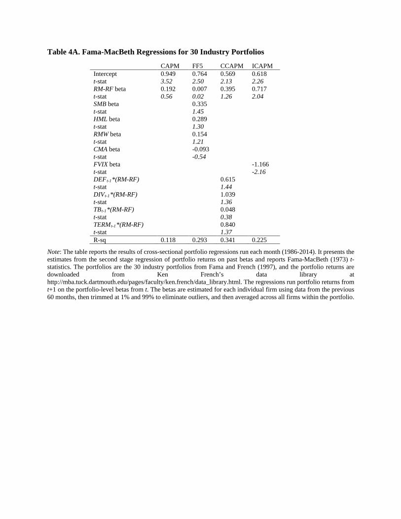
Table 4A. Fama-MacBeth Regressions for 30 Industry Portfolios

CAPM FF5 CCAPM ICAPM Intercept 0.949 0.764 0.569 0.618 t-stat 3.52 2.50 2.13 2.26 RM-RF beta 0.192 0.007 0.395 0.717 t-stat 0.56 0.02 1.26 2.04 SMB beta 0.335 t-stat 1.45 HML beta 0.289 t-stat 1.30 RMW beta 0.154 t-stat 1.21 CMA beta -0.093 t-stat -0.54 FVIX beta -1.166 t-stat -2.16 DEFt-1*(RM-RF) 0.615 t-stat 1.44 DIVt-1*(RM-RF) 1.039 t-stat 1.36 TBt-1*(RM-RF) 0.048 t-stat 0.38 TERMt-1*(RM-RF) 0.840 t-stat 1.37 R-sq 0.118 0.293 0.341 0.225

Note: The table reports the results of cross-sectional portfolio regressions run each month (1986-2014). It presents the estimates from the second stage regression of portfolio returns on past betas and reports Fama-MacBeth (1973) t-statistics. The portfolios are the 30 industry portfolios from Fama and French (1997), and the portfolio returns are downloaded from Ken French’s data library at http://mba.tuck.dartmouth.edu/pages/faculty/ken.french/data_library.html. The regressions run portfolio returns from t+1 on the portfolio-level betas from t. The betas are estimated for each individual firm using data from the previous 60 months, then trimmed at 1% and 99% to eliminate outliers, and then averaged across all firms within the portfolio.

35

Table 5A. GRS Test for Alternative Portfolio Sets

Panel A. 25 Size/market-to-book sorted portfolios CAPM FF3 ICAPM CCAPM FF5

Stat 4.757 4.738 5.037 4.259 3.698 p-value 0.000 0.000 0.000 0.000 0.000

Panel B. 25 Size/momentum sorted portfolios

CAPM FF3 ICAPM CCAPM FF5 Stat 2.868 2.963 2.632 2.292 2.396 p-value 0.000 0.000 0.000 0.001 0.000

Panel C. 25 Size/reversal sorted portfolios


Panel D. 25 Size/profitability sorted portfolios


Panel E. 25 Size/investment sorted portfolios


Note: The table reports the results of the test with the null hypothesis that the alphas of all portfolios mentioned in the panel name are jointly zero in the time-series full-sample model named in the column heading. For example, the top left cell performs, in full 1986-2014 sample, 25 regressions of excess returns to each of the portfolios from five-by-five annual sorts on size and book-to-market on excess market return, and tests if all 25 intercepts are jointly zero. The returns to the portfolio sets, the detailed descriptions of the sorting variables, and the sorting procedure are available from Ken French’s data library at http://mba.tuck.dartmouth.edu/pages/faculty/ken.french/data_library.html.

36

Table 6A. Joint Significance of the ICAPM/CCAPM factors for Alternative Portfolio Sets

Panel A. 25 Size/market-to-book sorted portfolios FVIX DEFt-1 DIVt-1 TBt-1 TERMt-1 Stat 8.875 3.982 1.095 1.550 2.047 p-value 0.000 0.000 0.346 0.048 0.003

Panel B. 25 Size/momentum sorted portfolios

FVIX DEFt-1 DIVt-1 TBt-1 TERMt-1 Stat 9.157 5.743 2.518 2.029 1.040 p-value 0.000 0.000 0.000 0.003 0.414

Panel C. 25 Size/reversal sorted portfolios


Panel D. 25 Size/profitability sorted portfolios


Panel E. 25 Size/investment sorted portfolios


Note: The table reports the results of the test with the null hypothesis that the FVIX betas (from ICAPM) or the interaction terms of the other four variables (DEF, DIV, TB, and TERM) with excess market return (from CCAPM) of all portfolios mentioned in the panel name are jointly zero. For example, the top right cell performs, in full 1986-2014 sample, 25 regressions of excess returns to each of the portfolios from five-by-five annual sorts on size and book-to-market on excess market return and its pairwise interactions with DEFt-1, DIVt-1, TBt-1, and TERMt-1, and tests if all 25 slopes on (RM-RF)*TERMt-1 are jointly zero. The returns to the portfolio sets, the detailed descriptions of the sorting variables, and the sorting procedure are available from Ken French’s data library at http://mba.tuck.dartmouth.edu/pages/faculty/ken.french/data_library.html.

37

Table 7A. Fama-MacBeth Regressions with Insurance and Financial Industry Factors

Panel A. 25 Size-BM Portfolios FF5 FF5+INS FF5+PL FF5+Life AFM FF5+AFM

Intercept 1.156 1.245 1.267 1.160 1.249 1.085 t-stat 4.53 4.89 4.95 4.59 4.31 3.90 RM-RF beta -0.042 -0.144 -0.145 -0.023 -0.227 -0.008 t-stat -0.13 -0.46 -0.46 -0.07 -0.67 -0.03 SMB beta 0.013 0.014 0.001 0.019 0.004 0.020 t-stat 0.08 0.08 0.01 0.11 0.02 0.10 HML beta 0.209 0.211 0.233 0.253 0.119 0.131 t-stat 1.06 1.08 1.21 1.28 0.61 0.68 RMW beta 0.182 0.220 0.241 0.202 0.143 t-stat 1.39 1.64 1.83 1.49 0.95 CMA beta 0.009 0.046 0.037 0.056 -0.018 t-stat 0.06 0.34 0.27 0.41 -0.13 INS beta 0.346 t-stat 1.20 PL beta 0.527 t-stat 1.46 Life beta 0.095 t-stat 0.26 FROE beta -1.012 -0.651 t-stat -1.69 -0.92 SPREAD beta 0.014 0.345 t-stat 0.06 1.40 R-sq 0.472 0.507 0.509 0.505 0.539 0.595

Panel B. 30 Industry Portfolios

FF5 FF5+INS FF5+PL FF5+Life AFM FF5+AFM Intercept 0.764 0.754 0.721 0.812 0.648 0.815 t-stat 2.50 2.53 2.48 2.67 1.93 2.64 RM-RF beta 0.007 0.002 0.035 -0.042 0.242 -0.132 t-stat 0.02 0.01 0.10 -0.11 0.57 -0.34 SMB beta 0.335 0.380 0.350 0.388 0.119 0.462 t-stat 1.45 1.67 1.54 1.66 0.49 1.89 HML beta 0.289 0.241 0.295 0.268 0.188 0.190 t-stat 1.30 1.04 1.31 1.16 0.76 0.83 RMW beta 0.154 0.099 0.102 0.085 -0.017 t-stat 1.21 0.78 0.81 0.64 -0.12 CMA beta -0.093 -0.023 -0.042 -0.097 0.025 t-stat -0.54 -0.12 -0.23 -0.52 0.12 INS beta 0.025 t-stat 0.07 PL beta 0.204 t-stat 0.42 Life beta -0.374 t-stat -0.77 FROE beta 0.700 0.291 t-stat 1.02 0.35 SPREAD beta -0.336 -0.066 t-stat -1.25 -0.23 R-sq 0.355 0.401 0.403 0.398 0.361 0.445

Note: The table reports the results of cross-sectional portfolio regressions run each month (1986-2014). It presents the estimates from the second stage regression of portfolio returns on past betas and reports Fama-MacBeth (1973) t-statistics. FF5 is Fama-French five-factor model in Fama and French (2015) and AFM is the model in Adrian, Friedman, and Muir (2016). In Panel A, the portfolios are five-by-five annual sorts on size and book-to-market, as in Fama and French (1993). In Panel B, the portfolios are the 30 industry portfolios from Fama and French (1997). INS (PL or Life) factor is the value-weighted returns to all publicly traded (P/L or life) insurance companies. The portfolio returns are downloaded from Ken French’s data library at http://mba.tuck.dartmouth.edu/pages/faculty/ken.french/data_library.html. The regressions run portfolio returns from t+1 on the portfolio-level betas from t. The betas are estimated for each individual firm using data from the previous 60 months, then trimmed at 1% and 99% to eliminate outliers, and then averaged across all firms within the portfolio.

38

Table 8A. GRS Test with Insurance Factors, Alternative Portfolio Sets

Panel A. 25 Size/market-to-book sorted portfolios FF5 FF5+INS FF5+PL FF5+Life AFM FF5+AFM Stat 3.698 3.586 3.62 3.658 4.254 3.463 p-value 0.000 0.000 0.000 0.000 0.000 0.000

Panel B. 25 Size/momentum sorted portfolios FF5 FF5+INS FF5+PL FF5+Life AFM FF5+AFM Stat 2.396 2.466 2.449 2.429 2.781 2.305 p-value 0.000 0.000 0.000 0.000 0.000 0.001

Panel C. 25 Size/reversal sorted portfolios FF5 FF5+INS FF5+PL FF5+Life AFM FF5+AFM Stat 1.175 1.215 1.207 1.192 1.728 1.276 p-value 0.259 0.222 0.230 0.243 0.018 0.174

Panel D. 25 Size/profitability sorted portfolios FF5 FF5+INS FF5+PL FF5+Life AFM FF5+AFM Stat 1.512 1.215 1.207 1.192 1.831 1.406 p-value 0.058 0.222 0.230 0.243 0.010 0.097

Panel E. 25 Size/investment sorted portfolios FF5 FF5+INS FF5+PL FF5+Life AFM FF5+AFM Stat 2.348 2.254 2.281 2.324 3.073 2.214 p-value 0.000 0.001 0.001 0.000 0.000 0.001

Note: The table reports the results of the test with the null hypothesis that the alphas of all portfolios mentioned in the panel name are jointly zero in the model named in the column heading. For example, the top left cell performs, in full 1986-2014 sample, 25 regressions of excess returns to each of the portfolios from five-by-five annual sorts on size and book-to-market on excess market return, SMB, HML, RMW, and CMA (FF5), and tests if all 25 intercepts are jointly zero. The cell next to it adds the value-weighted return to all publicly traded insurance companies (INS factor) to FF5, re-estimates the 25 regressions and again tests if all intercepts are jointly zero. The next two cells in Panel A replace INS factor by value-weighted returns to P/L and life insurers (PL factor and Life factor), redo the regressions, and perform the same test. The last two cells in Panel A replace FF5 in the first cell with AFM model and FF5 augmented with the additional AFM factors (FROE and SPREAD), redo the regressions, and perform the same test. The returns to the portfolio sets, the detailed descriptions of the sorting variables, and the sorting procedure are available from Ken French’s data library at http://mba.tuck.dartmouth.edu/pages/faculty/ken.french/data_library.html.

39

Table 9A. Other Types of Insurers Panel A. Accident and Health Insurers Panel B. All Other Insurers

CAPM FF5 AFM CCAPM ICAPM CAPM FF5 AFM CCAPM ICAPM RM-RF 0.90*** 1.03*** 0.90*** 0.65** -0.21 1.11*** 1.31*** 1.12*** 0.29 0.17 (0.06) (0.06) (0.06) (0.27) (0.25) (0.07) (0.07) (0.07) (0.33) (0.32) SMB 0.05 -0.00 0.28*** 0.31*** (0.09) (0.08) (0.11) (0.10) HML 0.55*** 0.04 0.73*** 0.36*** (0.12) (0.11) (0.14) (0.13) RMW 0.50*** 0.45*** (0.12) (0.15) CMA -0.33** 0.17 (0.17) (0.20) FROE 0.04 0.08* (0.04) (0.04) SPREAD 0.62*** 0.73*** (0.09) (0.11) FVIX -0.84*** -0.70*** (0.18) (0.23) DEFt-1*(RM-RF) 0.14 0.03 (0.12) (0.15) DIVt-1*(RM-RF) 0.35*** 0.49*** (0.10) (0.12) TBt-1*(RM-RF) -1.33** -1.17* (0.56) (0.69) TERMt-1*(RM-RF) -0.22** 0.02 (0.10) (0.13) Alpha 0.16 -0.13 0.14 0.02 -0.24 0.03 -0.52* -0.14 -0.17 -0.30 (0.26) (0.25) (0.24) (0.26) (0.27) (0.33) (0.31) (0.28) (0.32) (0.34) Adj R-sq 0.415 0.507 0.539 0.444 0.448 0.406 0.522 0.573 0.454 0.420 Obs 348 348 348 347 347 348 348 348 347 347

Panel C. Accident and Health Insurers Betas Recessions Expansion Difference Median as cutoff point 1.049*** 0.773*** 0.276*** (0.014) (0.014) (0.020) Top and bottom 25% as cutoff point 1.123*** 0.684*** 0.439*** (0.021) (0.021) (0.030) Panel D. All Other Insurers Betas Recessions Expansion Difference Median as cutoff point 1.332*** 0.942*** 0.390*** (0.023) (0.023) (0.032) Top and bottom 25% as cutoff point 1.407*** 0.788*** 0.618*** (0.030) (0.030) (0.042)

Note: Panels A and B show the regression results based on CAPM, FF5, AFM, CCAPM, and ICAPM for Accident and Health insurers (A/H insurers, SIC codes 6320-6329) and All Other Insurers (any insurers that are not P/L insurers (6330-6331), life insurers (6310-6311), or A/H insurers). The insurance portfolio returns are value-weighted. RM-RF is the market risk premium, SMB is the difference in the returns of small and large portfolios, and HML is the difference in the returns of high and low book-to-market portfolios. RMW is the difference in the returns of robust and weak (high and low) operating profitability portfolios, and CMA is the difference in the returns of conservative and aggressive (low and high) investment portfolios. FROE is the return spread between high and low ROE financial firms, and SPREAD is the return spread between financial and non-financial firms. DEF is default spread, DIV is dividend yield, TB is the 30-day Treasury bill rate, and TERM is term spread. FVIX is the factor-mimicking portfolio that mimics the changes in VIX index, which measures the implied volatility of the S&P100 stock index options. Panels C and D label the month as expansion or recession based on whether the predicted market risk premium is below or above in-sample median (median as cutoff point), or whether the predicted market risk premium is in the bottom or top quartile of its in-sample distribution (top and bottom 25% as cutoff point). We measure expected market risk premium as the fitted part of the regression 𝑅𝑅𝑅𝑅𝑖𝑖−𝑅𝑅𝑅𝑅𝑖𝑖 = 𝑏𝑏𝑖𝑖0 + 𝑏𝑏𝑖𝑖1𝐷𝐷𝐷𝐷𝑅𝑅𝑖𝑖−1 + 𝑏𝑏𝑖𝑖2𝐷𝐷𝐷𝐷𝐷𝐷𝑖𝑖−1 + 𝑏𝑏𝑖𝑖3𝑇𝑇𝐷𝐷𝑅𝑅𝑅𝑅𝑖𝑖−1 + 𝑏𝑏𝑖𝑖4𝑇𝑇𝑇𝑇𝑖𝑖−1 + 𝜀𝜀. Obs reports the number of months in the regressions. Standard errors appear in brackets. ∗∗∗, ∗∗, and ∗ denote statistical significance at the 1, 5, and 10 percent levels, respectively.

Table 10A. FVIX Exposures of 48 Fama-French (1997) Industry Portfolios

Agric-RF Food-RF Soda-RF Beer-RF Smoke-RF Toys-RF Fun-RF

Books-RF

Hshld-RF Clths-RF

RM-RF 0.689** -0.685*** -0.462 -0.808*** -0.756** 0.750*** 1.914*** 0.998*** 0.023 0.379 (0.287) (0.178) (0.313) (0.214) (0.327) (0.257) (0.247) (0.181) (0.165) (0.235) FVIX -0.064 -0.964*** -0.968*** -1.086*** -1.041*** -0.221 0.429** -0.018 -0.519*** -0.538*** (0.210) (0.130) (0.229) (0.157) (0.239) (0.188) (0.180) (0.133) (0.121) (0.172) Alpha 0.206 -0.012 -0.082 0.066 0.316 -0.244 0.251 -0.158 0.001 -0.143 (0.309) (0.192) (0.337) (0.231) (0.351) (0.277) (0.265) (0.195) (0.178) (0.252) Adj R-sq 0.292 0.446 0.310 0.393 0.209 0.486 0.632 0.646 0.529 0.562 Obs 347 347 347 347 347 347 347 347 347 347

Hlth-RF MedEq-RF

Drugs-RF

Chems-RF

Rubbr-RF Txtls-RF

BldMt-RF Cnstr-RF Steel-RF

FabPr-RF

RM-RF 0.404 0.911*** -0.161 0.787*** 0.974*** 1.313*** 0.700*** 1.143*** 2.667*** 1.580*** (0.286) (0.181) (0.184) (0.183) (0.204) (0.323) (0.204) (0.240) (0.255) (0.282) FVIX -0.332 0.042 -0.675*** -0.190 -0.065 0.086 -0.331** -0.048 0.914*** 0.383* (0.209) (0.132) (0.135) (0.133) (0.149) (0.236) (0.149) (0.175) (0.187) (0.206) Alpha -0.079 0.303 0.144 0.040 0.074 0.036 -0.116 -0.151 0.022 -0.072 (0.308) (0.195) (0.198) (0.196) (0.220) (0.348) (0.219) (0.258) (0.275) (0.303) Adj R-sq 0.336 0.561 0.499 0.652 0.607 0.440 0.645 0.593 0.657 0.454 Obs 347 347 347 347 347 347 347 347 347 347

Mach-RF ElcEq-RF

Autos-RF Aero-RF Ships-RF Guns-RF Gold-RF

Mines-RF Coal-RF Oil-RF

RM-RF 1.632*** 0.968*** 1.532*** 0.030 0.690** -0.448 0.838 1.514*** 2.132*** 0.194 (0.189) (0.177) (0.278) (0.217) (0.316) (0.297) (0.568) (0.330) (0.530) (0.226) FVIX 0.275** -0.205 0.198 -0.739*** -0.275 -0.772*** 0.328 0.315 0.755* -0.387** (0.138) (0.129) (0.203) (0.158) (0.231) (0.217) (0.416) (0.241) (0.388) (0.165) Alpha 0.101 0.071 -0.142 -0.167 -0.078 0.118 0.112 0.327 0.561 0.145 (0.203) (0.190) (0.299) (0.233) (0.341) (0.319) (0.612) (0.355) (0.571) (0.243) Adj R-sq 0.723 0.739 0.544 0.569 0.390 0.201 0.024 0.388 0.209 0.367 Obs 347 347 347 347 347 347 347 347 347 347

Util-RF Telcm-RF

PerSv-RF

BusSv-RF

Comps-RF

Chips-RF

LabEq-RF

Paper-RF

Boxes-RF

Trans-RF

RM-RF -0.358* 0.543*** 0.382 2.100*** 2.805*** 2.795*** 2.469*** 0.415** 0.425* 0.313* (0.183) (0.162) (0.234) (0.167) (0.257) (0.241) (0.201) (0.185) (0.228) (0.175) FVIX -0.583*** -0.282** -0.443*** 0.619*** 1.086*** 0.999*** 0.882*** -0.383*** -0.410** -0.466*** (0.134) (0.118) (0.171) (0.122) (0.188) (0.176) (0.147) (0.135) (0.167) (0.128) Alpha 0.082 -0.095 -0.387 0.325* 0.316 0.375 0.309 -0.092 0.003 -0.099 (0.197) (0.174) (0.251) (0.180) (0.277) (0.260) (0.216) (0.199) (0.245) (0.189) Adj R-sq 0.260 0.651 0.503 0.773 0.629 0.688 0.714 0.593 0.514 0.625 Obs 347 347 347 347 347 347 347 347 347 347

Whlsl-RF Rtail-RF

Meals-RF

Banks-RF Insur-RF RlEst-RF Fin-RF

Other-RF

RM-RF 0.724*** 0.374** -0.106 0.153 -0.226 1.750*** 1.754*** 0.977*** (0.142) (0.167) (0.177) (0.201) (0.174) (0.288) (0.172) (0.238) FVIX -0.146 -0.451*** -0.713*** -0.690*** -0.866*** 0.523** 0.325** -0.101 (0.104) (0.122) (0.129) (0.147) (0.127) (0.210) (0.125) (0.174) Alpha -0.079 -0.014 -0.099 -0.332 -0.327* -0.229 0.166 -0.483* (0.153) (0.180) (0.190) (0.217) (0.187) (0.310) (0.185) (0.257) Adj R-sq 0.707 0.666 0.583 0.629 0.639 0.439 0.774 0.555 Obs 347 347 347 347 347 347 347 347 Note: This table reports the ICAPM with FVIX regression results for all 48 industries defined by Fama-French (1997), available on http://mba.tuck.dartmouth.edu/pages/faculty/ken.french/Data_Library/det_48_ind_port.html. RM-RF is the market risk premium, and FVIX is the factor-mimicking portfolio that mimics the changes in VIX index. Obs reports the number of months in the regressions. Standard errors appear in brackets. ∗∗∗, ∗∗, and ∗ denote statistical significance at the 1, 5, and 10 percent levels, respectively.

41

Table 11A. Factor-Mimicking Regressions of CatLoss and the CombRat

Historical (1) (2) Historical (3) (4) Sensitivity CatLoss Sensitivity CombRat Quintiles VW EW Quintiles VW EW Quint1-RF 0.007 0.045 Quint1-RF 0.287* -0.067 (0.091) (0.128) (0.170) (0.277) Quint2-RF -0.012 -0.134 Quint2-RF 0.011 0.654 (0.131) (0.231) (0.217) (0.540) Quint3-RF -0.016 -0.028 Quint3-RF -0.311 -0.369 (0.124) (0.235) (0.282) (0.602) Quint4-RF 0.004 0.189 Quint4-RF 0.101 -0.276 (0.141) (0.278) (0.266) (0.582) Quint5-RF -0.013 -0.084 Quint5-RF -0.136 0.024 (0.077) (0.125) (0.157) (0.234) Constant 1.959*** 1.952*** Constant 0.005 -0.076 (0.319) (0.339) (0.660) (0.708) Adj. R-sq -0.044 -0.041 Adj. R-sq -0.013 -0.034 Obs 104 104 Obs 104 104

Note: This table performs the standard factor-mimicking regression with inflation-adjusted catastrophic losses (CatLoss) (in columns 1 and 2) or change in combined ratio (ΔCombRat) (in columns 3 and 4) on the left-hand side and excess returns to value-weighted (VW) and equal-weighted (EW) quintile portfolios based on the historical stock sensitivity to catastrophic losses and change in combined ratio, respectively. RF is risk-free rate. Standard errors appear in brackets. ∗∗∗, ∗∗, and ∗ denote statistical significance at the 1, 5, and 10 percent levels, respectively.

42

Table 12A. CatLoss Mimicking Portfolio: Alphas and Betas

(1) (2) (3) (4) (5) (6) (7) (8) CAPM FF3 Carhart FF5 CAPM FF3 Carhart FF5 Panel A. Value-Weighted Returns Panel B. Equal-Weighted Returns RM-RF -0.029*** -0.030*** -0.029*** -0.030*** -0.017*** -0.017*** -0.016*** -0.016*** (0.001) (0.000) (0.000) (0.001) (0.002) (0.002) (0.002) (0.002) SMB 0.003*** 0.003*** 0.003*** -0.012*** -0.012*** -0.013*** (0.001) (0.001) (0.001) (0.003) (0.003) (0.003) HML -0.004*** -0.004*** -0.003*** -0.007*** -0.007*** -0.010*** (0.001) (0.001) (0.001) (0.003) (0.003) (0.004) Mom 0.003*** 0.001 (0.000) (0.002) RMW -0.002 -0.001 (0.001) (0.004) CMA -0.002 0.008 (0.001) (0.005) Alpha -0.003 -0.002 -0.004** -0.001 -0.008 -0.005 -0.006 -0.007 (0.002) (0.002) (0.002) (0.002) (0.008) (0.008) (0.008) (0.008) Adj. R-sq 0.909 0.927 0.936 0.927 0.214 0.272 0.270 0.274 Obs 312 312 312 312 312 312 312 312

Note: This table reports the alphas and betas of the factor-mimicking portfolios on inflation-adjusted catastrophic losses in the CAPM, FF3, Carhart, and FF5 models. The factor-mimicking portfolios in Panels A and B are the fitted part from the regressions in columns 1 and 2 in Table 11A less the constant, respectively. RM-RF is the market risk premium, SMB is the difference in the returns of small and large portfolios, HML is the difference in the returns of high and low book-to-market portfolios, RMW is the difference in the returns of robust and weak (high and low) operating profitability portfolios, CMA is the difference in the returns of conservative and aggressive (low and high) investment portfolios, and Mom is the return differential from investing long in past winners and shorting past losers. Standard errors appear in brackets. ∗∗∗, ∗∗, and ∗ denote statistical significance at the 1, 5, and 10 percent levels, respectively.

43

Table 13A. ΔCombRat Mimicking Portfolio: Alphas and Betas

(1) (2) (3) (4) (5) (6) (7) (8) CAPM FF3 Carhart FF5 CAPM FF3 Carhart FF5 Panel A. Value-Weighted Returns Panel B. Equal-Weighted Returns RM-RF 0.012 0.002 -0.013 -0.016 -0.010* -0.011** -0.015** -0.009 (0.009) (0.009) (0.009) (0.010) (0.005) (0.006) (0.006) (0.006) SMB 0.049*** 0.052*** 0.038*** 0.020*** 0.021*** 0.024*** (0.013) (0.012) (0.014) (0.008) (0.008) (0.008) HML -0.015 -0.031** 0.034* 0.012 0.009 0.008 (0.013) (0.013) (0.019) (0.008) (0.008) (0.011) Mom -0.045*** -0.011** (0.008) (0.005) RMW -0.052*** 0.013 (0.020) (0.012) CMA -0.088*** 0.002 (0.027) (0.016) Alpha -0.051 -0.049 -0.009 -0.002 -0.007 -0.013 -0.003 -0.019 (0.040) (0.039) (0.038) (0.041) (0.023) (0.023) (0.023) (0.024) Adj. R-sq 0.002 0.049 0.134 0.086 0.008 0.029 0.040 0.027 Obs 312 312 312 312 312 312 312 312

Note: This table reports the alphas and betas of the factor-mimicking portfolios on change in combined ratio in the CAPM, FF3, Carhart, and FF5 models. The factor-mimicking portfolios in Panels A and B are the fitted part from the regressions in columns 3 and 4 in Table 11A less the constant, respectively. RM-RF is the market risk premium, SMB is the difference in the returns of small and large portfolios, HML is the difference in the returns of high and low book-to-market portfolios, RMW is the difference in the returns of robust and weak (high and low) operating profitability portfolios, CMA is the difference in the returns of conservative and aggressive (low and high) investment portfolios, and Mom is the return differential from investing long in past winners and shorting past losers. Standard errors appear in brackets. ∗∗∗, ∗∗, and ∗ denote statistical significance at the 1, 5, and 10 percent levels, respectively.

44

Table 14A. Underwriting Cycles in the Intertemporal CAPM (CatLoss)

(1) (2) (3) (4) (5) (6) (7) (8) (9) (10) (11) (12) RM-RF 0.87*** 0.04 0.87*** -0.27 -0.64*** -0.27 1.07*** 0.88*** 1.07*** 0.52*** 0.41* 0.52*** (0.05) (0.14) (0.05) (0.17) (0.19) (0.17) (0.04) (0.14) (0.04) (0.18) (0.21) (0.18) SMB -0.12** -0.11* -0.12** -0.08 -0.07 -0.08 (0.06) (0.06) (0.06) (0.06) (0.06) (0.06) HML 0.52*** 0.50*** 0.52*** 0.54*** 0.52*** 0.54*** (0.08) (0.08) (0.08) (0.07) (0.08) (0.08) RMW 0.32*** 0.31*** 0.32*** 0.22*** 0.22*** 0.22*** (0.08) (0.08) (0.08) (0.08) (0.08) (0.08) CMA 0.07 0.06 0.07 0.00 -0.00 0.00 (0.11) (0.11) (0.11) (0.11) (0.11) (0.11) FVIX -0.87*** -0.68*** -0.87*** -0.39*** -0.37*** -0.39*** (0.13) (0.13) (0.13) (0.13) (0.13) (0.13) FCatLoss -29.05*** -21.39*** -6.31 -4.44 (4.72) (4.76) (4.42) (4.42) CatLoss 0.01 0.04 0.01 0.01 (0.07) (0.06) (0.05) (0.05) Alpha 0.15 0.05 0.14 -0.28 -0.26 -0.35 -0.20 -0.20 -0.21 -0.33* -0.32* -0.35* (0.20) (0.19) (0.23) (0.19) (0.19) (0.23) (0.16) (0.16) (0.20) (0.17) (0.17) (0.20) Ad. R-sq 0.546 0.594 0.544 0.603 0.626 0.602 0.719 0.720 0.718 0.727 0.727 0.726 Obs. 312 312 312 312 312 312 312 312 312 312 312 312

Note: This table reports the regression results including the catastrophic losses factor into the three models from Tables 2 (CAPM, FF5, ICAPM) and FF5 augmented with FVIX (FF6) for all the publicly traded insurance companies. The results of estimating the four models are in columns 1, 4, 7, and 10, respectively. The catastrophic losses factor is added to the models in columns 2, 5, 8, and 11. In columns 3, 6, 9, and 12 factors is replaced by the variable it mimics (inflation-adjusted catastrophic losses). The left-hand side variable is the value-weighted returns to all insurance companies. RM-RF is the market risk premium, SMB is the difference in the returns of small and large portfolios, HML is the difference in the returns of high and low book-to-market portfolios, RMW is the difference in the returns of robust and weak (high and low) operating profitability portfolios, and CMA is the difference in the returns of conservative and aggressive (low and high) investment portfolios. FVIX is the factor-mimicking portfolio that mimics the changes in VIX index, which measures the implied volatility of the S&P100 stock index options. FCatLoss is the factor-mimicking portfolio that mimics the inflation-adjusted catastrophic losses, namely, the catastrophic losses factor. CatLoss is the variable that FCatLoss mimics, which is the inflation-adjusted catastrophic losses. Since FCatLoss and CatLoss are available from 1989, all regressions are from 1989 to 2014. Obs reports the number of months in the regressions. Standard errors appear in brackets. ∗∗∗, ∗∗, and ∗ denote statistical significance at the 1, 5, and 10 percent levels, respectively.

45

Table 15A. Cost of Equity Estimates

Panel A. All Insurers Year COE Estimates Sum-beta COE Estimates

CAPM (1)

FF5 (2)

CCAPM (3)

ICAPM (4)

AFM (5)

FF6 (6)

CAPM (7)

FF5 (8)

CCAPM (9)

ICAPM (10)

AFM (11)

FF6 (12)

1997 11.994 12.216 5.951 16.718 11.672 13.263 11.945 12.506 5.901 17.780 10.727 10.808 1998 12.779 14.289 4.672 17.523 12.873 14.938 13.080 16.887 4.651 20.305 13.330 15.997 1999 12.419 18.952 3.086 20.442 13.859 20.236 12.977 21.254 2.904 22.000 14.538 21.260 2000 11.906 20.945 4.439 26.400 15.825 23.420 12.808 21.380 4.451 26.495 17.029 21.555 2001 9.657 21.487 3.893 21.658 16.769 23.516 9.851 22.530 3.795 21.426 17.717 22.466 2002 8.369 19.120 2.617 17.007 14.797 19.800 8.647 20.089 2.591 17.214 15.946 19.650 2003 7.230 17.214 5.090 14.783 14.385 17.552 7.445 16.456 5.482 15.506 15.795 16.510 2004 6.505 15.434 6.109 15.399 13.353 16.706 6.848 13.771 5.140 16.528 14.587 14.532 2005 6.038 12.966 3.958 10.190 12.234 13.540 6.430 12.023 3.251 11.716 12.751 12.176 2006 7.324 10.693 4.437 8.481 8.772 10.934 7.824 12.827 4.189 9.636 10.208 12.199 2007 9.165 11.261 4.123 10.402 10.409 12.186 9.422 14.428 4.134 11.424 11.410 13.918 2008 10.291 10.032 2.994 11.136 9.615 10.574 10.571 10.626 2.985 11.407 8.915 10.381 2009 11.343 12.360 18.136 12.287 11.708 12.472 11.267 13.926 18.246 12.486 9.486 12.868 2010 10.704 8.470 28.765 11.064 9.839 8.895 10.644 10.398 28.963 10.718 8.669 10.326 2011 9.787 6.779 11.648 10.199 8.780 7.412 9.625 8.443 12.118 9.525 7.664 8.787 2012 8.852 5.627 8.532 9.229 8.030 6.224 8.644 7.555 8.778 8.504 6.872 7.846 2013 8.453 5.057 7.486 8.787 7.659 5.767 8.294 6.971 8.407 7.913 8.178 7.243 2014 7.152 5.017 6.520 7.314 6.296 5.377 6.530 5.678 6.002 5.365 7.029 5.677 Avg. 9.443 12.662 7.359 13.834 11.493 13.490 9.603 13.764 7.333 14.219 11.714 13.567

Panel B. P/L Insurers Year COE Estimates Sum-beta COE Estimates

CAPM (1)

FF5 (2)

CCAPM (3)

ICAPM (4)

AFM (5)

FF6 (6)

CAPM (7)

FF5 (8)

CCAPM (9)

ICAPM (10)

AFM (11)

FF6 (12)

1997 10.648 9.464 5.678 18.315 9.929 11.888 9.574 8.651 5.578 16.618 7.805 9.625 1998 11.805 11.888 4.689 19.712 11.531 14.399 11.332 13.566 4.662 19.785 11.485 14.298 1999 11.324 18.926 3.109 22.797 13.192 22.213 11.325 20.335 2.918 21.473 13.270 20.721 2000 10.988 21.363 4.444 27.601 16.926 24.995 11.957 20.786 4.468 25.172 16.972 20.636 2001 8.989 21.305 3.985 22.197 17.326 23.918 9.510 22.005 3.420 20.393 18.050 21.795 2002 7.822 17.832 2.692 17.367 14.632 18.765 8.246 18.160 2.595 16.372 15.055 17.480 2003 6.864 16.262 5.483 15.366 14.428 16.772 7.094 14.368 6.407 14.926 14.478 14.516 2004 6.364 14.410 5.854 16.533 13.368 16.293 6.824 11.777 4.974 16.641 13.496 13.201 2005 5.956 12.300 3.179 11.214 11.715 13.289 6.121 10.437 2.555 11.461 10.884 10.692 2006 7.518 9.825 4.087 9.605 7.939 10.334 7.390 12.191 4.031 8.941 10.241 11.048 2007 9.521 11.564 4.282 11.594 10.770 12.267 9.338 15.360 4.129 11.457 11.814 14.154 2008 9.465 10.251 3.040 10.695 8.332 10.766 9.443 11.125 2.914 10.220 7.270 10.640 2009 9.228 10.666 16.867 10.099 7.942 10.756 8.854 9.055 17.073 8.542 6.037 9.114 2010 8.421 5.710 22.910 8.464 6.319 5.937 8.107 4.692 21.954 6.269 4.495 4.763 2011 7.437 3.665 9.419 7.593 5.030 4.082 6.982 2.888 9.207 4.871 3.349 2.652 2012 6.528 2.523 7.077 6.759 4.404 2.926 6.039 1.880 6.700 3.939 2.557 1.552 2013 6.076 2.334 6.179 6.186 4.405 2.721 5.581 1.409 6.808 2.579 3.795 0.569 2014 5.085 3.323 5.264 6.857 4.362 4.603 3.839 3.375 4.605 3.342 4.526 3.458 Avg. 8.336 11.312 6.569 13.831 10.142 12.607 8.198 11.225 6.389 12.389 9.754 11.162

46

Panel C. Life Insurers Year COE Estimates Sum-beta COE Estimates

CAPM (1)

FF5 (2)

CCAPM (3)

ICAPM (4)

AFM (5)

FF6 (6)

CAPM (7)

FF5 (8)

CCAPM (9)

ICAPM (10)

AFM (11)

FF6 (12)

1997 12.664 19.831 6.094 20.394 15.631 21.997 13.636 22.230 6.209 25.200 15.612 22.828 1998 12.954 20.359 4.687 20.298 16.195 21.538 14.304 24.044 4.648 27.910 16.517 25.598 1999 12.745 18.533 3.127 18.932 14.808 18.359 14.436 22.383 2.664 26.066 15.422 24.864 2000 12.307 18.656 4.420 24.111 13.600 19.274 13.331 21.076 4.379 28.194 15.208 23.378 2001 10.415 19.815 3.499 20.132 15.095 20.536 10.415 22.570 3.879 22.259 16.841 22.799 2002 9.357 19.151 2.895 16.202 15.393 19.366 9.914 22.796 2.880 18.552 18.721 22.790 2003 8.476 17.795 6.139 14.330 15.370 17.824 9.161 20.235 5.127 17.229 19.848 20.137 2004 7.727 16.669 7.151 14.683 15.001 16.868 8.281 17.026 5.537 17.885 18.581 16.765 2005 7.223 13.389 5.656 9.315 13.863 13.130 8.337 14.921 4.957 13.619 17.103 15.027 2006 8.262 11.207 4.734 7.388 11.009 10.709 10.231 12.375 4.058 11.906 13.500 12.815 2007 9.571 10.252 4.177 8.243 10.219 9.703 10.873 10.547 4.462 11.391 12.797 10.320 2008 11.935 10.693 3.060 11.230 13.788 10.634 12.384 7.958 3.223 11.174 14.088 7.750 2009 17.882 18.525 24.145 17.902 22.526 18.672 19.255 27.730 24.827 23.168 21.371 23.803 2010 17.920 15.643 53.297 17.627 19.897 16.433 19.367 23.457 62.724 22.755 22.162 22.898 2011 16.981 13.658 20.048 16.584 18.462 14.664 18.069 18.928 23.070 21.098 20.171 21.311 2012 16.148 11.488 13.989 15.503 17.449 12.479 16.987 17.134 14.931 19.550 19.460 19.538 2013 16.335 10.883 11.819 16.215 15.526 12.432 17.583 18.292 12.467 22.503 19.373 22.358 2014 13.639 10.041 10.093 9.267 11.498 7.761 14.288 13.135 7.587 9.290 14.357 13.021 Avg. 12.363 15.366 10.502 15.464 15.296 15.688 13.381 18.713 10.979 19.431 17.285 19.333

Note: This table shows the value-weighted cost of equity (COE) estimates for all the publicly traded insurers, P/L insurers, and life insurers based on CAPM, FF5, CCAPM, ICAPM, AFM, and FF6 from 1997 to 2014 in columns 1-6. Columns 7-12 report the COE estimates based on the sum-beta approach. For each year, the annual COE estimate is the cumulative monthly COE estimates from January to December of that year. Avg. shows the average COE across the full sample period from 1997 to 2014.

47

Table 16A. Asset-Pricing Model Performance Comparison using Equal-Weighted Insurer Returns

Panel A. All Insurers Panel B. P/L Insurers Panel C. Life Insurers CAPM FF5 CCAPM ICAPM CAPM FF5 CCAPM ICAPM CAPM FF5 CCAPM ICAPM

RM-RF 0.81*** 0.89*** 0.64*** 0.39** 0.71*** 0.80*** 0.32** 0.05 1.01*** 1.10*** 0.87*** 0.80*** (0.03) (0.03) (0.15) (0.15) (0.03) (0.03) (0.15) (0.14) (0.05) (0.05) (0.20) (0.23) SMB 0.43*** 0.30*** 0.46*** (0.04) (0.05) (0.07) HML 0.59*** 0.46*** 0.99*** (0.05) (0.06) (0.09) RMW 0.17*** 0.19*** -0.05 (0.06) (0.06) (0.09) CMA 0.01 0.07 -0.10 (0.08) (0.09) (0.13) FVIX -0.31*** -0.50*** -0.16 (0.11) (0.11) (0.17) DEFt-1*(RM-RF) 0.09 -0.02 0.69*** (0.07) (0.07) (0.09) DIVt-1*(RM-RF) 0.25*** 0.26*** 0.21*** (0.06) (0.06) (0.07) TBt-1*(RM-RF) -1.33*** -0.59* -2.52*** (0.32) (0.32) (0.41) TERMt-1*(RM-RF) -0.07 -0.00 -0.24*** (0.06) (0.06) (0.08) Alpha 0.29* -0.01 0.17 0.13 0.25* -0.03 0.12 -0.00 0.20 -0.09 0.14 0.11 (0.16) (0.12) (0.15) (0.16) (0.15) (0.13) (0.15) (0.16) (0.24) (0.19) (0.19) (0.25) Adj R-sq 0.613 0.805 0.675 0.622 0.560 0.704 0.606 0.592 0.518 0.720 0.712 0.518 Obs 348 348 347 347 348 348 347 347 348 348 347 347

Note: This table shows the regression results based on CAPM, FF5, CCAPM, and ICAPM for all the publicly traded insurance companies, P/L insurers, and life insurers. The insurance portfolio returns are equal-weighted. RM-RF is the market risk premium, SMB is the difference in the returns of small and large portfolios, HML is the difference in the returns of high and low book-to-market portfolios, RMW is the difference in the returns of robust and weak (high and low) operating profitability portfolios, and CMA is the difference in the returns of conservative and aggressive (low and high) investment portfolios. We use four macroeconomic/business cycle variables as conditioning variables in the CCAPM, which include default spread (DEF), defined as the yield spread between Moody’s Baa and Aaa corporate bonds, dividend yield (DIV), defined as the sum of dividend payments to all CRSP stocks over the previous 12 months divided by the current value of the CRSP value-weighted index, Treasury bill rate (TB), which is the 30-day T-bill rate, and term spread (TERM), defined as the yield spread between the ten-year and the one-year T-bond. In the ICAPM, FVIX is the factor-mimicking portfolio that mimics the changes in VIX index, which measures the implied volatility of the S&P100 stock index options. Obs reports the number of months in the regressions. Standard errors appear in brackets. ∗∗∗, ∗∗, and ∗ denote statistical significance at the 1, 5, and 10 percent levels, respectively.

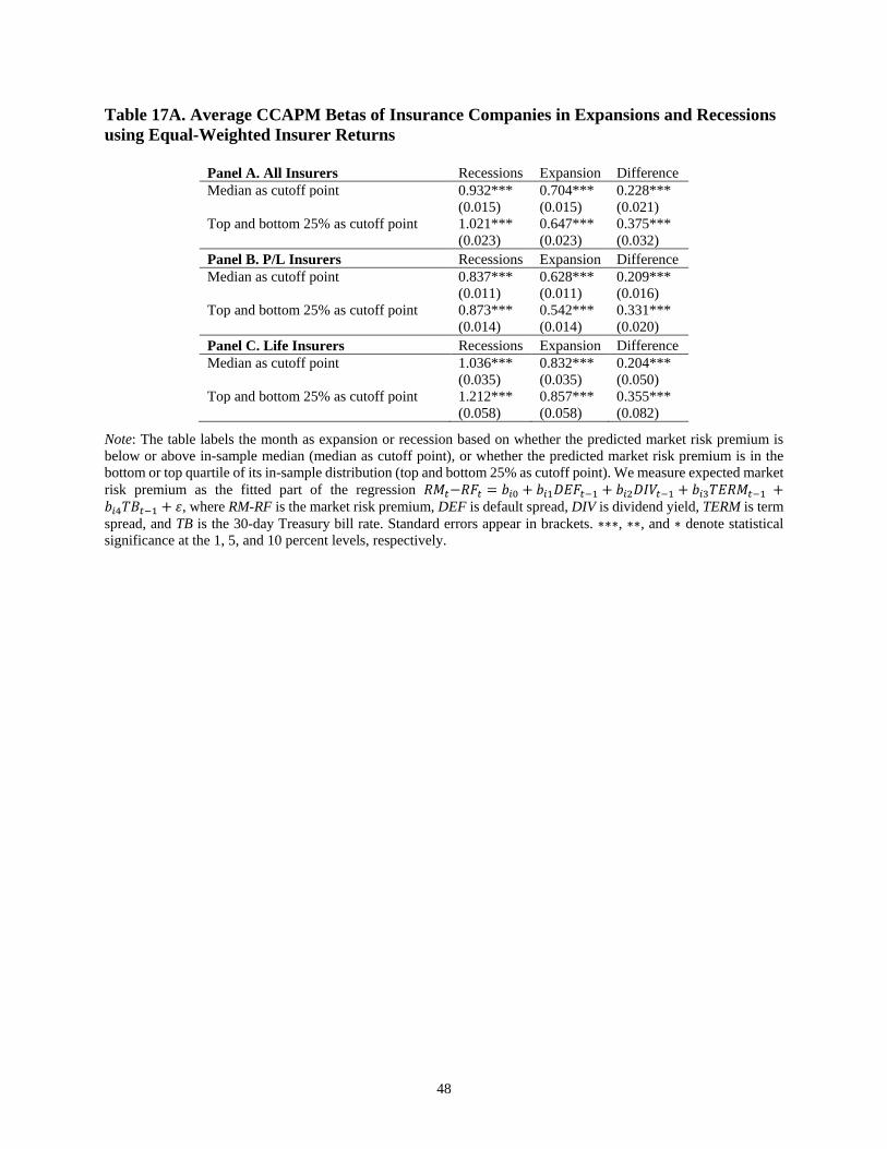
48

Table 17A. Average CCAPM Betas of Insurance Companies in Expansions and Recessions using Equal-Weighted Insurer Returns

Panel A. All Insurers Recessions Expansion Difference Median as cutoff point 0.932*** 0.704*** 0.228*** (0.015) (0.015) (0.021) Top and bottom 25% as cutoff point 1.021*** 0.647*** 0.375*** (0.023) (0.023) (0.032) Panel B. P/L Insurers Recessions Expansion Difference Median as cutoff point 0.837*** 0.628*** 0.209*** (0.011) (0.011) (0.016) Top and bottom 25% as cutoff point 0.873*** 0.542*** 0.331*** (0.014) (0.014) (0.020) Panel C. Life Insurers Recessions Expansion Difference Median as cutoff point 1.036*** 0.832*** 0.204*** (0.035) (0.035) (0.050) Top and bottom 25% as cutoff point 1.212*** 0.857*** 0.355*** (0.058) (0.058) (0.082)

Note: The table labels the month as expansion or recession based on whether the predicted market risk premium is below or above in-sample median (median as cutoff point), or whether the predicted market risk premium is in the bottom or top quartile of its in-sample distribution (top and bottom 25% as cutoff point). We measure expected market risk premium as the fitted part of the regression 𝑅𝑅𝑅𝑅𝑖𝑖−𝑅𝑅𝑅𝑅𝑖𝑖 = 𝑏𝑏𝑖𝑖0 + 𝑏𝑏𝑖𝑖1𝐷𝐷𝐷𝐷𝑅𝑅𝑖𝑖−1 + 𝑏𝑏𝑖𝑖2𝐷𝐷𝐷𝐷𝐷𝐷𝑖𝑖−1 + 𝑏𝑏𝑖𝑖3𝑇𝑇𝐷𝐷𝑅𝑅𝑅𝑅𝑖𝑖−1 +𝑏𝑏𝑖𝑖4𝑇𝑇𝑇𝑇𝑖𝑖−1 + 𝜀𝜀, where RM-RF is the market risk premium, DEF is default spread, DIV is dividend yield, TERM is term spread, and TB is the 30-day Treasury bill rate. Standard errors appear in brackets. ∗∗∗, ∗∗, and ∗ denote statistical significance at the 1, 5, and 10 percent levels, respectively.

49

Table 18A. Underwriting Cycles in the Intertemporal CAPM using Equal-Weighted Insurer Returns (Combined Ratio Change)

(1) (2) (3) (4) (5) (6) (7) (8) (9) (10) (11) (12) RM-RF 0.81*** 0.80*** 0.81*** 0.39** 0.35** 0.38** 0.90*** 0.90*** 0.90*** 0.39*** 0.40*** 0.37*** (0.04) (0.04) (0.04) (0.16) (0.16) (0.16) (0.03) (0.03) (0.03) (0.14) (0.14) (0.14) SMB 0.41*** 0.40*** 0.41*** 0.45*** 0.44*** 0.45*** (0.04) (0.04) (0.04) (0.04) (0.04) (0.04) HML 0.57*** 0.56*** 0.57*** 0.59*** 0.58*** 0.59*** (0.06) (0.06) (0.06) (0.06) (0.06) (0.06) RMW 0.18*** 0.20*** 0.18*** 0.10 0.11* 0.09 (0.06) (0.06) (0.06) (0.06) (0.06) (0.06) CMA 0.08 0.11 0.09 0.02 0.05 0.02 (0.08) (0.08) (0.08) (0.08) (0.08) (0.08) FVIX -0.32*** -0.34*** -0.32*** -0.36*** -0.36*** -0.37*** (0.12) (0.12) (0.12) (0.09) (0.09) (0.10) FCombRat 0.27 0.37 0.29* 0.29* (0.24) (0.24) (0.17) (0.17) ΔCombRat 0.01 0.02 0.02 0.02 (0.03) (0.03) (0.02) (0.02) Alpha 0.38** 0.40** 0.39** 0.23 0.23 0.22 0.05 0.05 0.05 -0.07 -0.07 -0.07 (0.17) (0.17) (0.17) (0.18) (0.18) (0.18) (0.12) (0.12) (0.12) (0.13) (0.13) (0.13) Adj R-sq 0.583 0.583 0.582 0.591 0.593 0.591 0.797 0.798 0.797 0.806 0.807 0.806 Obs 312 312 312 312 312 312 312 312 312 312 312 312

Note: This table reports the regression results including the combined ratio factor (FCombRat) into the three models from Tables 2 (CAPM, FF5, and ICAPM) and FF5 augmented with FVIX (FF6) for all the publicly traded insurance companies. The results of estimating these four models are in columns 1, 4, 7, and 10, respectively. The combined ratio factor is added to the models in columns 2, 5, 8, and 11. In columns 3, 6, 9, and 12 each factor is replaced by the variable it mimics (change in combined ratio). The left-hand side variable is the equal-weighted returns to all the publicly traded insurance companies. RM-RF is the market risk premium, SMB is the difference in the returns of small and large portfolios, HML is the difference in the returns of high and low book-to-market portfolios, RMW is the difference in the returns of robust and weak (high and low) operating profitability portfolios, and CMA is the difference in the returns of conservative and aggressive (low and high) investment portfolios. FVIX is the factor-mimicking portfolio that mimics the changes in VIX index, which measures the implied volatility of the S&P100 stock index options. FCombRat is the factor-mimicking portfolio that mimics the changes in combined ratio, namely, the combined ratio factor. ΔCombRat is the variable that FCombRat mimics, which is the change in combined ratio. Since FCombRat and ΔCombRat are available from 1989, all regressions are from 1989 to 2014. Obs reports the number of months in the regressions. Standard errors appear in brackets. ∗∗∗, ∗∗, and ∗ denote statistical significance at the 1, 5, and 10 percent levels, respectively.

50

Table 19A. Equal-Weighted Cost of Equity Estimates

Panel A. All Insurers Panel B. P/L Insurers Year COE Estimates Year COE Estimates

CAPM (1)

FF5 (2)

CCAPM (3)

ICAPM (4)

CAPM (1)

FF5 (2)

CCAPM (3)

ICAPM (4)

1997 10.100 13.305 5.609 9.923 1997 9.364 14.095 5.474 13.724 1998 10.616 13.784 4.824 10.314 1998 10.064 14.755 4.840 13.054 1999 10.889 16.993 3.717 14.741 1999 10.114 16.502 3.785 15.343 2000 10.145 18.300 4.762 16.806 2000 9.496 17.774 4.801 16.764 2001 8.716 18.295 4.465 14.427 2001 8.205 17.288 4.474 14.241 2002 7.872 17.615 2.565 11.937 2002 7.392 16.310 2.523 11.772 2003 7.061 16.852 2.646 10.330 2003 6.682 15.791 2.655 10.304 2004 6.624 15.803 4.913 10.118 2004 6.424 14.976 4.730 10.443 2005 6.811 14.285 4.307 8.029 2005 6.598 13.248 3.977 8.214 2006 7.893 13.091 4.377 6.340 2006 7.672 12.412 4.239 6.458 2007 9.665 13.871 4.336 7.118 2007 9.441 13.747 4.416 7.055 2008 10.969 14.035 3.089 10.597 2008 9.972 13.349 3.105 9.723 2009 11.396 13.714 15.623 13.173 2009 9.158 12.354 12.057 10.823 2010 11.022 10.663 25.549 12.481 2010 8.548 9.311 16.132 10.014 2011 10.134 9.420 11.643 11.808 2011 7.650 7.805 9.481 9.431 2012 9.151 7.907 8.784 10.635 2012 6.549 6.403 7.046 8.053 2013 8.762 6.801 7.556 10.256 2013 6.059 5.946 5.660 7.544 2014 8.080 8.626 6.665 7.775 2014 5.765 8.185 5.283 6.823

Average 9.217 13.520 6.968 10.934 Average 8.064 12.792 5.815 10.544

Panel C. Life Insurers Year COE Estimates

CAPM (1)

FF5 (2)

CCAPM (3)

ICAPM (4)

1997 10.304 16.495 5.547 13.542 1998 10.690 16.468 4.801 13.788 1999 10.796 17.820 3.764 15.325 2000 10.121 17.852 4.828 16.622 2001 9.023 18.163 4.366 14.174 2002 8.381 17.841 2.822 11.789 2003 7.837 18.080 3.846 10.443 2004 7.465 17.511 5.549 10.316 2005 7.553 14.401 4.576 7.608 2006 8.737 12.467 4.239 5.537 2007 10.422 14.811 4.352 6.148 2008 12.257 15.551 3.113 10.795 2009 16.893 23.341 27.065 21.150 2010 16.952 17.628 50.852 21.213 2011 15.865 15.901 19.267 20.255 2012 14.871 14.283 14.201 19.039 2013 14.950 12.463 12.636 20.191 2014 12.349 10.917 9.326 11.442

Average 11.415 16.222 10.286 13.854 Note: This table shows the equal-weighted cost of equity (COE) estimates for all the publicly traded insurers, P/L insurers, and life insurers based on CAPM, FF5, CCAPM, and ICAPM from 1997 to 2014 in columns 1-4, respectively. For each year, the annual COE estimate is the cumulative monthly COE estimates from January to December of that year. Average shows the average COE across the full sample period from 1997 to 2014.

Appendices For “Estimating the Cost of Equity Capital for ...

Documents

Transcript of Appendices For “Estimating the Cost of Equity Capital for ...