Apparent Emissivity in the Base of a Cone

Cosmin DAN, Gilbert DE MEY

University of Ghent

Belgium

Overview

1. Introduction

2. Description of the problem

3. Configuration factors computation

4. Apparent emissivity computation

5. Genetic algorithms (GA)

6. Results

7. Conclusions

Introduction

• Why to calculate the apparent emissivity?- Build a black-body- What kind of shapes has usually a black body- Find the optimal shape- Solve the radiative energy balance equations- Write a computer program for apparent

emissivity computation- Use a genetic algorithm optimization method

Description of the problem

• Circular cavities– Diffuse-gray surfaces– Known distribution of the temperature– Only radiative heat transfer– Known inner walls emissivity not depending

on temperature– Known geometrical dimensions– Unknown apparent emissivity

Description of the problem

εapp

εapp

εapp εapp

Description of the problem

• The boundary integral equation

Sdrr

rqr

rrTrT

r

rqS

244 coscos

)]()(

)(1)([)(

)(

)(

|| rr

r

r )(rq

)(rq

Description of the problem

• The net radiation method

)()(1

1

44

1

4

1

N

jjiji

N

jjiijjj

N

j j

jji

j

ij TTFFTqF

ji

jiij en wh0

en wh1

i j

z

R

Description of the problem

• The net radiation method

iiij CqA

)( and )1( for

)1(1 for

1

44ij

N

jjijiii

jijj

i

jii

FTTεcFε

ε

εji

Fεji

a

– Gauss elimination method

Configuration factors computation

22

21

12 )(41

2

RRXXF

A1

A2

r2

r1

h

h

rR

h

rR

R

RX 2

21

121

22 and with

11

Configuration factors computation

R

x

Ai1 Ai2 Aj1 Aj2

Ai

Aj

)()(1

1222211211 ijijjijijji

ji FFAFFAA

F

Apparent emissivity

– Radiative heat flux leaving the cavity– Radiative heat flux that would leave the cavity

if it were a blackbody– Computation of the total heat flux for different

particular cases with specified temperature– Find the highest value for apparent emissivity

• Same length• Same open area• Different shapes for cavity

Genetic algorithms

– System for function optimisation – Adaptive search – iterative procedures

– Variables = structures xi, population

– Vector of parameters to the objective function

),...,( 21 npppf

11001110...)( 211 1000 nppptx

10001p

)(),...(),()( 21 txtxtxtP N

Genetic algorithms

Yes Printout results

Initialize population P(t)

Evaluate objective function

Complete terminate criteria

Select the best members

Mate and mutate

Replace old members

No

Genetic algorithms

• Two steps to create a new population– Selection of the best members for replication– Alteration of the selected members using

genetic operators:• Crossover

– Two parents → two offspring's– 100011001111 and 011100110011 → 100011000011

and 011100111111

• Mutation– Alteration of one ore more bites in parent structure– 100011001111 → 100010001111

Genetic algorithms

Genetic Algorithm Software

Generate initial population Calculate the objective function

(εapp)

Return the value of the objective function for each structure

Generate the new population according with performances

Check the terminate criteria

Return results

Genetic algorithms

R

z P1(z1,R1)

P2(z2,R2)

P3(z3,R3) P0(z0,R0)

P1’(z1

’,R1’)

•Termination criteria:Acceptable approximate solutionFixed total number of evaluations

Results

0.00E+00

1.00E-10

2.00E-10

3.00E-10

4.00E-10

5.00E-10

6.00E-10

7.00E-10

1 51 101 151 201 251 301

Number of the surface (-)

Sum

mat

ion

-rel

ativ

e er

ror

(%)

NiFN

jij ...1 where1

1

Results

• Configuration factors from each surface to the open area:– Disk-to-disk method– Monte Carlo integration method

• Configuration factors from each surface to all the others surfaces– Formula for differential configuration factors

between two ring elements– The approximated formula e-2z

Results

0

0.2

0.4

0.6

0.8

0.00 0.20 0.40 0.60 0.80 1.00z/L

Fij

0

0.1

0.2

0.3

0.4

0.5

0.6

cone angle 60°

cone angle 15°

Results

0

0.005

0.01

0.015

0.02

0.025

0 0.5 1 1.5 2 2.5 3 3.5 4

Cylinder length [m]

Con

figur

atio

n fa

ctor

s [-

]

differentialformula

exponentialaproximation

disk-to-disk

Results

0.00E+00

1.00E-05

2.00E-05

3.00E-05

4.00E-05

5.00E-05

6.00E-05

0 0.5 1 1.5 2 2.5 3 3.5 4

Cylinder length [m]

Rel

ativ

e di

ffer

ence

[%

]

disk-to-disk and differentialformula

Results

0.00

0.01

0.01

0.02

0.02

0.03

0 0.2 0.4 0.6 0.8 1

Cylinder length [-]

Con

figur

atio

n fa

ctor

s [-

]

disk-to-disk middleareadisk-to-disk lastareadisk-to-disk firstarea

Results

0

20

40

60

0 0.2 0.4 0.6 0.8 1z/L

q[W

/m^2

]

cone-cylinder

cone

cylinder

Results

0

1

2

3

4

5

6

7

0 0.2 0.4 0.6 0.8 1z/L

Abs

olut

e di

ffere

nce

[W/m

^2]

cylinder and cone-cylinder

cylinder and cone

Results

0.2

0.4

0.6

0.8

1

0 2 4 6 8 10 12 14 16 18 20L/R

App

aren

t em

issi

vity

cone cylinder

εwall=0.25

εwall=0.50

εwall=0.75

Results

0.945

0.950

0.955

0.960

0.965

0.970

0.975

0 500 1000 1500

Trials number

App

aren

t em

issi

vity

Results

• L=z3=30 cm; • 0 ≤ z1 ≤ L; εwall=0.9• R1=R2=15 cm • εapp=0.971 for z1=0.91 cm• R1=R2=5 cm• εapp=0.975 for z1=0.01 cm

R

z P1(z1,R1)

P2(z2,R2)

P3(z3,R3) P0(z0,R0)

P1’(z1

’,R1’)

• L=z2=z3=z4=30 cm; • 0 ≤ z1 ≤ L; εwall=0.9• R1=R2=10 cm; R3=2.5 cm • εapp=0.9986 for z1=0.01 cm

R

z P1(z1,R1)

P2(z2,R2)

P4(z4,R4) P0(z0,R0)

P1’(z1

’,R1’)

P3(z3,R3)

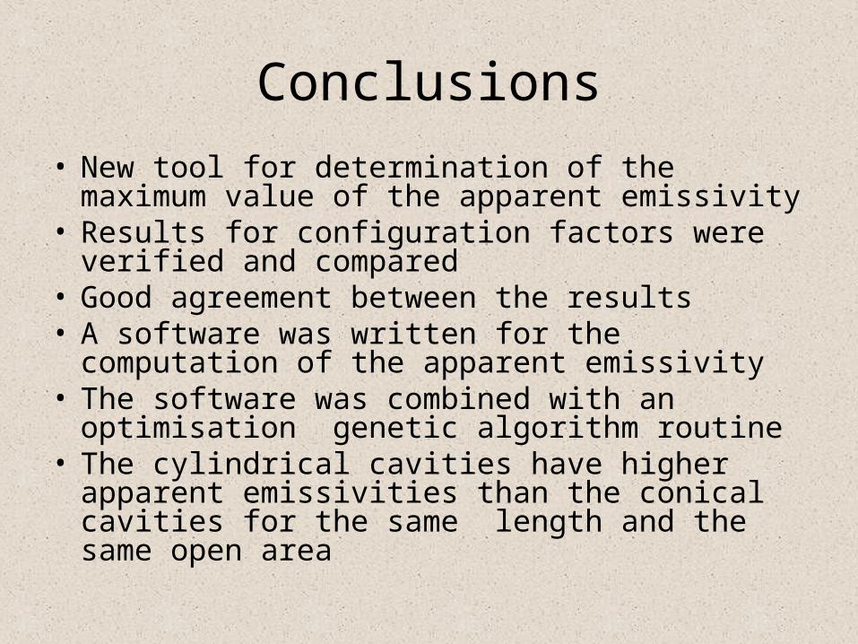
Conclusions

• New tool for determination of the maximum value of the apparent emissivity

• Results for configuration factors were verified and compared

• Good agreement between the results • A software was written for the computation of the

apparent emissivity• The software was combined with an optimisation

genetic algorithm routine• The cylindrical cavities have higher apparent

emissivities than the conical cavities for the same length and the same open area