Aportaciones al cálculo del ÍNDICE DE VALOR BIOLÓGICO ...€¦ · Loya-Salinas, D.H. y Escofet,...

APORTACIONES AL CALCULO DEL INDICE DE VALOR BIOLOGICO (Sanders, 1960)

CONTRIBUTION TO THE CALCULATION OF THE BIOLOGICAL VALUE INDEX (Sanders, 1960)

Daniel H. Laya-Salinas Anamarfa Escofet

Departamento de Ecologia Centro de Investigación Científica y de

Educación Superior de Ensenada (CICESE) Dirección en México: Apartado Postal 2732, Ensenada, B.C., 22830

U.S. Mailing Address: P.O. Box 4844, San Ysidro, CA. 92073

Loya-Salinas, D.H. y Escofet, A. (1990). Aportaciones al c5lculo del Indice de Valor Biol6gico (Sanders, 1960). Contriiution to the calculation of the Biological Value Index (Sanders, 1960). Ciencias Marinas, X(2): 97-115.

RESUMEN

Se discute la utilidad de combinar la constancia espacio-temporal y las abundancias de las especies como herramienta para descriiir la estructura por especies en comunidades marinas, con especial énfasis en bentos, y se presenta una guía detallada del algoritmo para el calculo del Indice de Valor Biológico o IVB (Sanders, 1960) el cual es un indicador de la dominancia global por especie, basado en rangos y puntajes. Se explica el modo de trabajar con los empates en el orden de abundancia y la influencia del patrón de dominancia muestral sobre la determinación del puntaje mrkimo. Por primeravez se presenta una fórmula del IVB y se recomiendausar el 95% de los individuos por muestra para eliminar los datos carentes de información relevante.

Se obsetvaron fuertes contrastes entre el orden de importancia general asignado por abundancia total, y aquel asignado por el IVB, pues este último evita la ordenación en base a datos puntuales dominantes pero poco representativos. Se recomienda que el uso del IVB incluya un análisis previo de clasificación numérica, y se discuten los efectos de la heterogeneidad del sustrato sobre el fndice.

Palabras clave: ecología marina, estructura comunitaria, rangos, puntajes, abundancias, fndice de valor biológico, constancia espacio-temporal.

ABSTRACT

The usefulness of combining the spatio-temporal constancy and abundances of the species as tools to describe the species structure in marine communities is discussed, with special emphasis on benthos. A detailed guide of the algorithm for the calculation of the Biological Value Index or BVI (Sanders, 1960) is also presented. The BVI indicates the overall dominance per species, based on ranks and points. The procedure of working with ties in the ranking of abundances and the influente of the sampling dominance pattem on the determination of the maximum score is explained. For the fiist time a formula of the BVI is presented and the use of 95% of the individuals per sample is recommended to elirninate data which lack relevant information.

97

http://dx.doi.org/10.7773/cm.v16i2.688

Key words: marine ecoloav. cornmunitv structure, ranks, points, abundances, biological value index, spatiotemporal con%ncy.

INTRODUCCION INTRODUCLION

Este trabajo es básicamente metodoló- gico, y se encuadra dentro del campo de la Ecología Estadística, disciplina que comprende los numerosos algoritmos cuantitativos que se ocupan en la exploración de patrones en comunidades bióticas (Ludwig y Reynolds, 1988).

This work is basically methodological and falls under the lield of statistical ecology, a subject which includes the numerous quantitative algorithms used in the study of pattems in biotic communities (Ludwig and Reynolds, 1988).

La composición de especies en una comunidad, o sea, la abundancia y tipo de las especies presentes, es una de sus caracterfsti- cas más obvias, y en los estudios descriptivos de comunidades se ha hecho cada vez más importante la identificación de las fluctua- ciones naturales en la abundancia de las especies componentes, incluyendo su amplitud y periodicidad (Andrewartha y Birch, 1982).

Species composition in a community, that is, the abundance and type of species present, is one of its most obvious charac teristics, and in descriptive studies of communities, the identification of natural fluctuations in the abundance of the species, includ- mg amplitude and periodicity, has become increasingly more important (Andrewartha and Birch, 1982).

Para la documentación de las fluctua- ciones en la organización de las comunidades es importante distinguir los cambios atribui- bles a factores inducidos (antropogénicos) o ajenos al medio ambiente (v.g., la influencia de fuertes disturbios producidos por un con- taminante), de aqudllos que son derivados de los ritmos y variaciones propias del sistema natural que se estudia (tales como ciclos estacionales y/o anuales), y que afectan al número de especies que son típicamente dominantes, ya que esos disturbios afectan la heterogeneidad espacial y temporal de los ecosistemas y consecuentemente las abundancias relativas de las especies presentes (Pickett y White, 1985).

In order to document the fluctuations in the organization of communities it is important to distinguish the changes attributable to induced factors (anthropogenic) or outside influentes on the environment (e.g. strong disturbances caused by pollutants) from those derived from rhythms and variations proper to the natural system under study (such as seasonal and/or annual cycles), and which affect the number of species which are typically dominant. Such disturbances affect the spatial and temporal heterogeneity of the ecosystems and, consequently, the relative abundances of the species present (Pickett and White, 1985).

Frecuentemente se usan datos de abundancias para estudiar la estructura comunitaria y sus variaciones en el tiempo. El caso más común de variaciones naturales corres- ponde con las estaciones climáticas, y cuando éstas ocurren (como sucede en la mayoría de las comunidades marinas), la selección de especies representativas de una comunidad en base a datos puntuales de abundancia no

Abundarme data are frequently used to study the community structure and its variation in time. Natural variations are usually caused by climatic seasons. When these occur (as happens in most marine communities), the selection of representative species from a community based on abundance data is not representative. Tools are needed which take into account the cyclic temporal changes in the dominance of the main species.

Loya-Salinas, D.H. y Escofet, A.- Aportaciones al calculo del Indice de Valor Biológico

Strong contrasts were observed behveen the rank assigned by total abundance and that assigned by BVI, since the latter avoids ranking based on dominant but less representative data. For the use of the BVI, an anlysis previous to the numerical classification is recornmendedand the effects of substrate heterogeneity on the index are discussed.

98

resulta representativa, requiriéndose de he rramientas que permitan esa selección inte grando los cambios cíclicos temporales en las dominancias de las especies principales.

Una forma sencilla de realizar la des- cripción de la estructura por especies se basa en la aplicación de rangos y puntajes, y es usada ampliamente en los estudios de ecología marina para ordenar la importancia de cada una de las especies (Fager, 1957; Sanders, 1960; Guille, 1971; Wattling, 1975; Richard- son, 1976; Milstein et al., 1976; Maurer et al., 1979; Pearson, 1975; Zarkanellas y Kattoulas, 1982; Elias, 1987) y también para ordenar los sitios de muestreo de acuerdo a variables ambientales (Sanders et al., 1980).

En sus trabajos en ecología bentónica, Sanders (1960) recalca que las abundancias son un criterio más valido que la biomasa para representar la estructura de una comunidad. Esto es debido a que la presencia de un animal grande que aparece en una muestra y que no es típico de esa muestra, puede alterar la distribución de la biomasa para esa muestra hasta en dos órdenes de magnitud; esto produce estimaciones de la estructura comunitaria con un sesgo asociado que será signl- ficativamente mayor que el permitido en este tipo de estudios.

La idea de sustituir las abundancias por rangos viene de bastantes años atrás, desde los trabajos realizados por Cole (1949) en estudios bent6nicos, quien observó que muestras de distinto tamaño tendrán un efecto despropor- cionado sobre los cálculos de las asociaciones entre especies, por los valores extremos que contienen. Ese efecto es encontrado muy frecuentemente al trabajar con conjuntos de poblaciones naturales, y se ha observado que la forma de contrastar la diferencia de los resultados obtenidos al trabajar con datos de biomasa o datos de conteos, es mediante la asignación de rangos a las especies para equiparar la importancia de cada muestra dentro de la comunidad.

Un antecedente significativo sobre el uso de los rangos para investigar la organización de las especies dentro de una comunidad (o sea, su estructura por especies) está en un trabajo de Fager (1957) sin embargo fue Sanders (1960) quien afinó la idea de un Indice

A simple method used to descri’be the species structure is based on the application of ranks and points. It is widely used in studies on marine ecology to rank each species in order of importance (Fager, 1957; Sanders, 1960; Guille, 1971; Wattling, 1975; Richardson, 1976; Milstein et al., 1976; Maurer et al., 1979; Pearson, 1975; Zarka- nellas and Kattoulas, 1982; Elias, 1987) and to put in order the sampling sites according to environmental variables (Sanders et al., 1980).

In his works on benthic ecology, Sanders (1960) stressed that abundances rather than biomass are a more valid criterion for the representation of the community structure. This is due to the fact that the presente of a large, atypical animal in a sample, may aher the biomass of that sample by two orders of magnitude. This produces estimates of the community structure with an associated bias which will be signilicantly higher than that allowed for this type of studies.

The idea of substituting abundances by ranks was proposed severa1 years ago, beginning with Cole% (1949) benthic studies. This author observed that samples of different sizes will have a disproportionate effect on the calculations of interspecifc associa- tions, due to their extreme values. That effect is often found while working with natural population assemblages, and it has been observed that the way to contrast the differ- ence in the results obtained while working with biomass data or counts, is through the allocation of ranks to species in order to compare the importance of each sample within the community.

A signiticant antecedent on the use of ranks to study the organization of species within a community (i.e., species structure) is found in a work by Fager (1957). However, it was Sanders (1960) who perfected the idea of an index based on points to determine the importance of species. In Mexico it has been known since 1983 as the Biologlcal Value Index (BVI) and its use was reported a year later (Beltr&n-Félix, 1984).

To calculate the BVI, a value of importance is assigned to each species in terms of its abundance in each sample and is

Laya-Salinas, D.H. y Escofet, A.- Aportaciones al calculo del Indice de Valor Biológico

99

basado en puntajes para ordenar la importancia de las especies. En M6xico se le conoce desde 1983 como “Indice de Valor Biológico o NB”, y fue hasta un año después cuando su uso fue reportado (Beltrán-Félix, 1984).

Para el calculo del IVB se asigna un valor de importancia a cada especie en función de su abundancia en cada muestra, y es expresada a manera de puntajes (o puntos). Primero se realiza una ordenación de las especies en cada muestra en base a la magnitud de su abundancia; la especie con mas abundancia en la muestra ocupa el primer lugar (rango= l), la segunda en orden de abundancia ocupa el segundo lugar (rango=2) y así sucesivamente. Sanders (1960) lo explica de la siguiente manera: “este factor se deter- mina asignando rangos del 1 al 10 a las especies por orden de abundancia dentro de cada muestra. A un rango de 1 le es dado un valor de 10 puntos; un rango de 2 equivale a 9 puntos; 3 es equivalente a 8 puntos, . . . . . . y un rango de 10 equivale a 1 punto. Por lo tanto si una especie ocupa el primer lugar en rango en 20 muestras, tendrá un valor de 200, o sea el máximo valor posible”.

Como puede observarse, esa explicación es muy sencilla en contenido y carente de información respecto a las dudas que puede encontrar el usuario al realizar los cíllculos (v.g.’ empates en las abundancias) y la forma de solucionarlas, por lo cual se procedió a investigar algunas opciones a cada paso de los cálculos del IVB para así formalizar su uti- lización en los trabajos de ecologia de comunidades marinas, con especial énfasis en bentos. La primera parte de los resultados se presenta en este trabajo.

Asimismo, tratando de solucionar algu- nos problemas que surgieron al usar el IVB, se procedió a estudiar su estructura, especial- mente las secciones de: (a) cómo defii la manera de trabajar con empates en los rangos y puntajes; (b) cómo determinar el valor del puntaje m&ximo en conjuntos de muestras con diferente dominancia; y (c) la presentación de un algoritmo completo para los c&ulos del fndice, incluyendo su fórmula.

A través de los usuarios del IVB nos hemos enterado de las dudas que se les presentan y de otras preguntas que han

given by way of points. First the species in each sample are ranked by abundance; the most abundant species in the sample occupies fust place (rank = l), the second in order of abundance occupies second place (rank=2) and so forth. Sanders (1960) explains it in the following way: ‘This factor is determined by ranking the species from 1 to 10 by abundarme within each sample. A rank of 1 is given a value of 10 points; a rank of 2 equals 9 points; 3 is equivalent to 8 points, . . . . . . and a rank of 10 equals one point. Thus if a @cies is i%iiked fust in 24l samples, it will have 200 points, the highest possible score”.

As can be seen, this explanation is very simple and lacks information regarding doubts which the user may expect to come across during the calculations (e.g. a tie in the abundances) and ways to solve them. For this reason, we proceded to study options in each step of the calculation of the BVI and thus formalize its use in ecological studies on marine communities, with special emphasis on benthos. The first part of the results are presented in this study.

Furthermore, in order to solve some problems arising from the use of the BVI, its structure was studied, especial@ (a) how to defmeprocedureswhen ties occur in ranks and points, (b) how to determine the maximum points in groups of samples with different dominance and (c) the presentation of a complete algorithm for the calculation of the index, including its formula.

From BVI users we have become aware of their doubts and other questions which have arisen. In this work we present an explanation of the BVI algorithm and discuss its advantages relative to the population parameter of total abundance, which is often used in ranking the importance of species in a community. In a forthcoming work we will deal with the uses of the BVI since 1983 as well as with a comparative statistical analysis between the BVI and other indices which attempt to estimate the importance of the specieswithin a community. As an example of those indices, that of spatial niche amplitude (Whiting and McIntire, 1985) and importance in the community (Stephens and Zerba, 1981) can be mentioned

LoyaSalinas, D.H. y Escofet, A.- Aportaciones al calculo del Indice de Valor Biológico

100


surgido. Este trabajo presenta una explicación del algoritmo del IVB y la discusión de sus ventajas respecto al parámetro poblacional de la abundancia total, el cual es usado fre cuentemente en la ordenación de la importancia de las especies en una comunidad. En un trabajo posterior se tratará de los usos que se han dado al IVB desde 1983 a la fecha, así como un análisis estadístico entre el IVB y otros fndices que tratan de estimar la importancia de las especies dentro de una comunidad. Como ejemplo de esos indices pueden mencionarse el de amplitud de nicho espacial (Whiting y McIntire, 1985) y el de importancia en la comunidad (Stephens y Zerba, 1981).

The BVI has been widely accepted in the field of marine ecology and the usefulness of the results obtained through its use has been confiied in research work carried out in several lields, such as: benthic infauna (Calderón-Aguilera, 1984), epiphytic diatoms in sea grasses (Siqueiros-Beltrones et al., 1985), ichthyofauna (Grijalva-Chan, 1985; Beltr&n-Félix et al., 1986; Ruiz-Campos, 1986), pelagic phytoplankton (Atilano-Silva, 1987), pelagic zooplankton (Jiménez-Pérez, 1987; Castro-Longoria and Hammann, 1989) and suprabenthonic zooplankton (Hem&ndez- Alfonso et al., 1987).

METHODOLOGY El IVB ha tenido bastante aceptación en

el ámbito de la ecología marina, y la utilidad de los resultados obtenidos a través de su uso ha sido comprobada ampliamente con la ayuda de investigaciones realizadas en varias disciplinas tales como: infauna bentónica (Calderón-Aguilera, 1984) diatomeas epifitas en pastos marinos (SiqueirosBeltrones et al., 1985) ictiofauna (Grijalva-Chan, 1985; Bel- trán-Félix et al., 1986; Ruiz-Campos, 1986) litoplancton pelágico (Atilano-Silva, 1987) zooplancton pelágico (Jiménez-Pérez, 1987; Castro-Longoria y Hammann, 1989) y zooplancton suprabentónico (Hernández-Alfonso et al., 1987).

The method is based on the calculation of the BVI for each species in the community and the final objective is to rank the species in order of importance based on the spatio-temporal constancy of their abundances, expressed through the BVI value.

METODGLOGIA

Globalmente, el procedimiento se basa en el calculo del IVB para cada especie en la comunidad, y el objetivo fmal es ordenar la importancia de las especies en base a la constancia espacio-temporal de sus abundancias, expresada mediante el valor del IVB.

The characteristics of the BVI can be summarized as a defmed sequence of operations. The complete procedure is explained below, and to facilitate the example Pam- plona-Salazar’s (1977) data will be used. These are shown in Appendix 1 (the data of four taza which were not identified to genus or species were removed). The calculation of the BVI consists of four general steps: (1) lists are prepared, (2) the number of species to be used is established, (3) points are assigned and (4) the BVI value per species is calculated.

1. Preparation oc lists

Las caracterlsticas del IVB pueden ser resumidas como una secuencia definida de operaciones. A continuación se explica el procedimiento completo de cálculo. Para fa- cilitar el ejemplo se usarán los datos de PamplonaSalazar (1977) mostrados en el Ap6ndice 1 (se eliminaron los datos de cuatro taza que no fueron identificados hasta género o especie). El Calculo del IVB consiste en cuatro pasos generales que son: (1) la preparación de planillas; (2) establecer el número de especies a utilizar; (3) asignación de puntajes; y (4) el c&lculo del valor del IVB por especie.

An individual list has to be prepared for each sample (sampling date or site). The species should be placed in decreasing order of their abundance value (ABU), and the results of the relative abundance per species @BR), the accumulative relative abundarme per species (ARA) and the rank (RAN) assigned to each one should be included. When there are no ties in the sample (two or more species with the same abundance), ranks are assigned in the same manner as explained by Sanders

w@).

In the infrequent case of ties in the ranking by abundarme, the same rank is assigned to both species and the next rank is

101

Laya-Salinas, D.H. y Escofet, A.- Aportaciones al c&ulo del Indice de Valor Biológico

Apéndice 1. Estructura temporal de la comunidad infaunal en un trarxcto de playa arenoso en la Bahfa de Todos Santos, B.C., entre julio de 1973 y mayo de 1974. Tomado de Pamplona-Salazar (1977) y atpresada como individuos/m2. Appendis 1. Temporal structure of the infaunal community in a sandy beach transect in Todos Santos Bay, B.C., behveen July 1973 and May 1974. Taken from Pamplona-Salazar (1977) and expressed as individuals/m2.

1973 1974

SEP NOV ENE MAR MAY

Syncheiidium sp. Ttidentella sp. Netine cbmtulus Nephtys califomiensis Glycem tenuis LIonm @dii Cbchestoidea benedicti Alchacimlysis sp. Armadillium SQ. Megalotvpus sp. Emetita anal* Ponthatpinia sp. Euwnus muctvnata Lepidqa californica Magelona califomica Hanstotina sp. Glycem dibmnchiata Atchaeavnysis maculata

2398 1626

1125 37 165

544 875 265 566 914 75

ll 251 958 90 59 155

149 266 101 16 69 96

0 0 5 69 0 5

0 16 0 0 0 0

811 1275 1343 7079 528 1990 1098 1274

1141 1540 118 53 404 170 58 90 106 646 133 118 42 5 5 15

133 79 162 245 160 37 522 111 91 16 208 283 48 30 0 0 96 27 0 10 ll 16 0 0 37 341 0 0 16 0 16 0 5 0 42 10 5 0 0 0 0 0 5 0 0 5 0 0

1. Preparaci6n de planillas

Para cada muestra (fecha de muestreo o localidad de muestreo) debe preparame una planilla individual presentando las especies por orden decreciente del valor de sus conteos de abundancia (ABU), incluyendo los resultados del cktlo ‘de la labundancia relativa por especie (ABR), la abundancia relativa acumu- lativa por especie (ARA), y el rango (RAN) asignado a ca& una. Cuando no hay empates en la muestra (dos especies o más con la misma abundancia), la asignación de rangos se realiza de la misma manera como lo explica sanders (1960).

Cuando hay empates en el orden por abundancia (caso menos frecuente), se asigna el mismo rango a las dos especies empatadas y

omitted. When three species are tied then the next hvo ranks are omitted and so forth (cfr. Dobbs, 1981). It is also neuxsary to include one last column where the individual points (PUN) assigned to each species will later be annotated, as the calculations advance. Table 1 shows the JuL73 (ftied) list lllustrating this procedure which, in spite of being easy, should be done carefully since all the following steps are based on these records. For example, note that since both Dunar gouldii and Ne#tys califomiensis have the same value of 7 points, the next specles, Glycem tenuis, is given a value of 5 points.

2. Number d species to be used in each sample

When the number of species is arbi- trarily chosen, considerable underestimation

102


se omite el rango siguiente, con tres especies empatadas se omiten los dos rangos siguientes, y así sucesivamente (cfr. Dobbs, 1981). Tam- bién es necesario incluir una última columna donde se anotará posteriormente el puntaje individual (PUN) asignado a cada especie en la muestra, a medida que se avance en los cálculos. La Tabla I muestra la planilla de JULJ3 (terminada) ilustrando este proce dimiento que, a pesar de ser sencillo, debe efectuarse cuidadosamente pues en estas planillas se basan todos los pasos siguientes; por ejemplo, nótese que al asignar el mismo puntaje (7) a las especies tiax goufdii y NepQs crJifomiensis, el siguiente puntaje (6) se pierde y se asigna el puntaje de 5 a la especie Glycem tenuis.

can occur. In samples with low dominance the number of species chosen may not reach a representative percentage of the total number of individuals in the samples and, therefore, the order of the species will be inefficient.

2. Nlmera de especies a utilizar en cada muestra

The number of species ln each sample to be considered in the overall calculations is defmed based on the general pattem of dominance of the community, represented by the degree of dominance in the samples which represent it. This criterion has been applied by users of the BVI, and up to 20 species have been considered in communities with low dominance (e.g. McCloskey, 1970) while 10 to ll species have been included in cases of high dominarme (e.g. Sanders, l%o, Richardson, 1976; Maurer and April, 1979; Maurer et al., 1979).

Cuando se elige un número de especies arbitrario, se puede incurrir en un error considerable de subestimación, debido a que en muestras con baja dominancia el número de especies seleccionado pueden no alcanzar a reunir un porcentaje representativo del nú- mero total de individuos en las muestras, y por lo tanto la ordenación de las especies será poa eficiente.

La forma de definir el número de especies de cada muestra a considerar en los cálculos globales se realiza en base al patrón general de dominancia de la comunidad, representado por el grado de dominancia en las muestras que la representan. Este criterio ha sido aplicado por los usuarios del IVB, pues en comunidades con baja dornlnanciar han sido consideradas hasta 20 especies (v.g.1 McCloskey, 197O).rnientras que 10 a ll espe cies fueron incluidas en casos de alta dominancia (v.g.: Sanders, l%o; Richardson, 1976; Maurer y April, lm, Maurer et al., 1979).

The selection of the number of species ls done automatically if, at the beginn@, instead of defining an absolute number of species to be used, a constant referente accumulatlve percentage (PAR) is defmed in relation to the total of the individuals in each sample. Since it refers to the dominance found in each of the samples, it will aut+ matically assign a lower or higher number of species per sample for the calculations of the BVI.

The dominance pattem in each sample can rapidly be estimated by obsetving the behaviour of the accumulative relative abundances (ARA) in the individual lists. This characteristic is shown in Table II. Typically, in communities with high dominarme few species make up a signillcant percentage of the total number of individuals (80% or more), whilst with low dominance a considerably large number of species ls required in order to reach a signifIcarn value of ARA.

La elección del número de especies se realiza automáticamente si en vez de definir al inicio un número absoluto de especies a utilizar, se define un porcentaje acumulativo de referencia (PAR) constante respecto al total de los individuos en cada muestra, que al estar referido a la dominancia encontrada en cada una de las muestq asignara automá- ticamente un menor o mayor número de especies por muestra para los cálculos del IVB.

A PAR of 95% is recommended since this criterion agrees with the data reduction process, whlch is almost routine in descrip tive studies of conununitks (Clifford and Stephenson, 1975; Boesch, lw7; Field et al., 1982) and which results ln the eliminatlon of redundant lnformation (genera@ the elimina- tion of rare specles). This is also strengthened by extensive studies like that of Smith (1976), who showed that the quantlty of lnformatlon eliminated per sample that can be tolerated

103

Loya-Winas, D.H. y Escofet, A.- Aportaciones al c6lculo del Indlce de Valor Biol6gico

Tabla 1. Planilla para la muestra de julio de 1973 mostrando (a) las especies ordenadas por abundancia (ABU), las abundancias relativas @BR), las abundancias relativas acumulativas (ARA), el rango (RAN) asignado a cada especie, la columna de los puntajes por especie (PUN); y (b) lado derecho de la misma planilla al sirnularse un empate en el orden por abundancia de las especies Lkmm gouldii y Nephrys calijbmiensis (se presenta ~510 la columna de los puntajes). Table 1. List for the July 1973 sample showing (a) the species in order of abundance (ABU), relative abundances @BR), accumulative relative abundances (ARA), rank given to each species (RAN) and points per species (PUN); and (b) right side of the same list when simulating a tie in the order of abundance of the spehes Llonax gouldii and Nepkys califmiensk (only the column of points is presented).

(4 Especie ABU ABR ARA RAN PUN I PRa Synchelidium sp. 2398 31.72 31.73 1 10 10 Tridentella sp. 2048 27.09 58.82 2 9 9 Amhaeomysis sp. 958 12.67 71.50 3 8 8 Donar gouldii 914 12.09 83.51 4 7 7 Nephtys califomiensis 544 7.19 90.79 5 6 7 Glycem ten& 265 3.50 94.29 6 5 5 Megalompus sp. 149 1.97 %.27 7 4 4 Emetita analoga 101 1.33 97.60 8 3 3 Pontharpinia sp. 69 0.91 98.52 9 2 2 Amwdillium sp. 59 0.78 99.29 10 1 1 Nerine cimztulus 37 0.49 99.79 11 0 0 Otchestoidea benedicti ll 0.14 99.93 12 0 0 Lepidopa @fornica 5 0.06 100.00 13 0 0

El patrón de dominancia en cada muestra puede estimarse rápidamente obser- vando el comportamiento de la columna de abundancias relativas acumulativas (ARA) en las planilhrs individuales; y esta característica se muestra en la Tabla II. ‘I”rpicamente, en comunidades con dominancia alta pocas especies acumulan un porcentaje signilicativo del número total de individuos (80% o más), mientras que con baja dominancia se re- quiere incluir un considerable número de especies para alcanzar un valor de ARA importante.

Se recomienda considerar un PAR del 95%, pues este criterio concuerda con el procedimiento de reducción de datos, el cual es casi de rutina en estudios descriptivos de comunidades (Clifford y Stephenson, 1975; Boesch, 1977; Field et al., 1982), y que resulta

without a signiflcant change in the pattem studied is approximately 5%. Quite often, the PAR is not exactly 95% in each sample and, in that case, the number of specles associated to the closest value of ARA but larger than 95% is chosen as the maximum number of species to be considered in that sample.

Through the examination of the ARA column in all the individual lists, it can be seen that the PAR (95%) is met by a different numbe-r of species in each sample. In Table II, which illustrates this step of the procedure, it can be observed that, for example, a 95% ARA value is obtained by seven, ten, six, seven and four species ln the JUL-73 to MAY-74 samples respectively (in other words, a minimum of four and a rnrcdmum of ten species obtained an ARA of 95% in the samples). This maximum value of N = 10 becomes important in the

104

Laya-Salinas, D.H. y Escofet, A.- Aportaciones al calculo del Indice de Valor Biolbgico

‘fabla II. Abundancias relativas acumulativas (ABA) calculadas en la preparación de las planillas individuales, para las seis fechas de muestreo. El signo + a la derecha de un valor de AR4 indica el número de especies que acumulan el 95% del total de individuos en cada muestra. La columna marcada con BAN indica el rango de las especies. Table II. Accumulative relative abundances (ABA) calculated in the preparation of the individual lists, for the six sampling dates. The + sign on the right of an ABAvalue indicates the number of species which make up 95% of the total of individuals in each sample. The column marked RAN indicates the rank of the species.

1973 1974

JUL SEP NOV ENE MAY

1 2

3 4 5 6 7 8 9

10 ll 12 13 14 15 16

31.73 58.83 71.50 83.68 90.79 94.29 96.27 t 97.61

98.52 99.30 99.79 99.93

100.00

30.13 31.12 50.98 53.23 67.28 67.63 77.69 78.65 82.62 83.01 87.27 86.64 98.33 89.53 93.28 92.15 94.98 94.63 %.65 t %.67+ 98.84 97.98 99.31 98.99 99.61 99.43 99.91 99.73

100.00 99.86 I 100.00

32.22 36.2n

57.15 65.79 77.79 79.86 88.25 85.47 93.77 89.84 %.52 t 93.42 97.88 96.60-t 98.48 98.17

98.88 99.30 99.32 99.73 99.58 99.86 99.84 100.00 99.92

100.00

76.22 89.93

92.98 95.62 + 96.89 98.08

99.05 99.62 99.78 99.89

100.00

en la eliminación de información redundante (generalmente la eliminación de especies raras), y es reforzado por trabajos extensos como el de Smith (1976) quien demostró que la cantidad de información eliminada por muestra que puede ser tolera& sin un cambio significativo en el patrón estudiado es del 5% aproximadamente. Muchas veces el PAR no se ajusta exactamente al 95% en cada muestra, y en ese caso el número de especies asociado al valor de AR4 más próximo pero mayor al 95% es seleccionado como el núme- ro máximo de especies a considerar en esa muestra.

following steps as it defines the maximum number of points (Pm& which will be assigned to the most numerically important species in each sample.

3. Abcation of points

The allocation of points to the species included in each sample is carried out in two possible ways, depending on the presente or absence of ties in the abundance counts of the species.

Mediante la impección de la columna de AR& en todas las planillas individuales se advierte que el PAR (95%) es reunido por un número diferente de especies en cada muestra. En la Tabla II, que ilustra este paso del

(a) Allocation of points in the absence of ties

Once the maximum number of species that obtained an approximate ARA value of 95% (greater/equal) is known, considering all

105


procedimiento, se observa por ejemplo que un valor de ARA del 95% es reunido por siete, diez, di% seis, siete y cuatro especies en las muestras de JUL73 a MAY-74 respectiva- mente (en otras palabras, un mInimo de cuatro especies y un m&rimo de diez reunieron un ARA del 95% en las muestras). Para los pasos siguientes este valor mkxirno de N= 10 adquiere importancia pues queda definido como el puntaje mkimo (Pm& que será asignado a la especie con mayor importancia numérica en cada muestra

3. Asignación de puntajes

La asignación de puntajes a las especies contenidas en cada muestra se realiza de dos maneras posibles, dependiendo de la presencia o ausencia de empates en los conteos de abundancia de las especies.

the samples, the user assigns that number as the maximum score to the most abundant speciea in each sample. This is an important requirement imposed by the folknving steps of the method, which are related to the mechanism of the tests of statistical signili- cance by ranks and which require the allocation of points relative to a foted hierarchic frame (Conover, 1980). That is, from here on only the most important N species in each sample (in this example N = 10) will be considered and the other species will be elirninated from the calculation of the BVI. In each sample, on allocating descending points, a value .of 1 point is reached and all the following species are allocated the value of 0, thus eliminating their effect on the overall calculations.

(a) Asignación de puntajes en ausencia de empates

Una vez conocido el número máximo de especies que reunió un valor aproximado de ARA del 95% (mayor/igual), considerando todas las muestras, el usuario asignara ese número como puntaje m&imo a la especie más abundante en cada muestra. Esto es un requerimiento importante impuesto por los pasos siguientes del método, que están rela- cionados con la mecánica de las pruebas de significancia estadística por rangos, y que requieren la ponderación de los puntajes respecto de un marco jekquico fijo (Conover, 1980). Es decir, de aquí en adelante se trabajará solamente con las N especies más abundantes en cada muestra (en este ejemplo N = 10) y las demás especies serán eliminadas del calculo del IVB; en cada muestra, al asignar puntajes descendentes se llega a puntajes de 1 y a todas las especiessiguientes se les asigna un puntaje de 0 con lo que se elimina su efecto en los c&xlos globales.

The selection of a maximum number of species can appear confusing since, once the number of species to be used has been found, this number reaches a percentage higher than 95% in some samples (Table II). This fact is frequent and is a result of the variation of the pattem of dominarme in the samples. In those cases, it should be remembered that the maximum number of species which reach 95% in the whole set of samples is used and, therefore, so that the maximum points be applied evenly to all the samples, in some of them more species than those which accumulate the PAR will be considered.

(b) Allocation of points in the presente of ties

When two or more species are tied in order of abundance, the same procedure as that for ranks is used. This consists of allocating the same score to the tied species and omitting the following point(s) (when there is a tie behveen two species the next value is omitted, between three species the next two values are omitted and so forth).

La elección de un número maxirno de especies puede parecer confuso pues una vez encontrado el número de especies a trabajar, en algunas muestras ese número reune un porcentaje más alto que el 95% (Tabla II); este hecho es muy frecuente y resulta de la variación del patrón de la dominancia en las muestras. En esos casos debe recordarse que se trabaja con el mkrno número de especies

When there are ties in ranks, there are ties in the score. In order to illustrate this point, the abundance of the fourth and fifth species (Euwnus mucnmata and Donax @dii) was equaled in Table 1 to forte a tie (this is shawn in the last column otthat table and will not be included in the calculations of the example). The comparison of the two

106

que en el conjunto de las muestras reune el 95% y como consecuencia, para que el puntaje máximo se aplique a todas las muestras por igual, en algunas de ellas se considerarán más especies de las que acumulan el PAR.

(b) Asignación de puntajes en presencia de empates

Los casos de empate en el lugar alcan- zado por dos o más especies por orden de abundancia se tratan con el mismo procedimiento usado con los rangos, consistente en asignar el mismo puntaje a las especies empatadas y omitir el/los siguientes puntajes (con dos especies empatadas se omite el puntaje siguiente; con tres especies empatadas se omiten los dos puntajes siguientes, y así sucesivamente).

Cuando hay empates en los rangos, se produce un empate en los puntajes. Con el propósito específico de ilustrar este punto, se igual6 la abundancia de las especies cuarta y quinta (Euzonus muctvnata y Donar gouldii) en la Tabla 1 para forzar un empate (esto se presenta en la última columna de esa tabla, y no se incluirá en los c&ulos del ejemplo). La comparación de las dos columnas de puntajes de la derecha en la Tabla 1 permite advertir que el efecto de la omisión del valor (o valores) del puntaje siguiente a un empate, es para no alterar los puntajes de las especies posicionadas por debajo del empate.

4. Cfilculo del valor final del IVB

Considerando una matriz de datos de dimensiones NE (número de especies) por NM (número de muestras), el valor fmal de IVB para cada especie se obtiene mediante la suma de todos los puntajes asignados a cada especie por el procedimiento explicado. Como puede apreciarse, la f6rmula del IVB es sencilla, y se presenta como parte del algoritmo general en la Figura 1. En el total de NE especies (i = lJW), para cada i-ksima especie se calcu- lar6 un IVBi que resulta de sumar los puntajes obtenidos por esa especie en el grupo de las NM muestras estudiadas (i = 1, NM).

En el proceso de operaciones necesarias primer0 se forma la matriz de conteos de abundancias de las especies (abur), con las especies posícíonadas en los d r onesy las

columns of points on the right of Table 1 shows that the value (or values) of the score following a tie should be omitted so as not to aher the points of the species positioned below the tie.

4. Calculation of the final BVI value

Considering a matrix of data of dimen- sions NE (number of species) by Nh4 (number of samples), the fmal BVI value for each species is obtained by adding all the points assigned to each species. As can be seen, the BVI formula is simple and is presented as par-t of the general algorithm in Figure 1. In the total of NE species (i=l, NE), for each i-th species, a BVIi will be calculated resulting from the sum of the points obtained for that species in the group of Nh4 samples studied (j = 1, NM).

In the process of necessary operations, fxst the abundance count matrix of the specie~ is formed (abuij), with the species placed in lines and the samples in columns. The lists are then prepared providing the necessary information for the allocation of points to the species in each sample and which in tum result in the formation of a second matrix, that of scores @unij). Both matrices are of dimension NJ?NM.

From the deftition of this formula it can be- inferred that the range of values resulting from the BVI is between a minimum of 0 and an indefinite maximum of points that is not fxed and which depends on the combination of two facts: the general pattem of dominance (expressed by the maximum score) and the number of samples obtained of that community (BVImâx = NWP,ax).

In our example, the species Nerine cimatulus obtained 0, 4, 10, 9, 4 and 3 points in the lists, re.sulting in a fmal value of BVI 130 points for that species. In the case of Sjmchelidium sp., a BVI = 57points is obtained based on values of 10, 10, 9, 8, 10 and 10 points (Table III).

DISCUSSION

Even though Sanders did not e+lciUy state it, the index works by balancing two

Laya-Salinas, D.H. y Escofet, A.- Aportaciones al c&lculo del Indice de Valor Biológico

107


MATRIZ DE

CONTEOS

(obuij 1,.

LISTA FINAL DE ESPECIES ORDENADAS POR VALOR DE IVB

-

i-i 2

-

N

MAFZ PUNTAJES

(Punij)

Figura 1. Algoritmo general del Indice de Valor Biológico (NB), a manera de diagrama de flujo, incluyendo su fórmula. Figure 1. General algorithm of the Biological Value Index (BVI), presented as a flux diagram, including its formula.

muestras en las columnas. A continuación se generan las planillas que proporcionan la información necesaria para asignar los puntajes a las especies en cada muestra, y que a su vez resultan en la formación de una segunda matriz, la de puntajes (puni). Las dos matrices son de dimensiones NE l hí.

Por la deftici6n de esta fórmula se deduce que el rango de valores que puede resultar del IVB esta entre un mfnimo de 0 y un mzkimo indefinido de puntos que no es fijo y que depende de la combinación de dos factores: el patrón general de dominancia (expresado por el puntaje nkirno) y el número de muestras obtenidas de esa comunidad (IVBmax = NM*Pm&.

En el ejemplo que estamos siguiendo, la especie Netine citmtuho obtuvo los puntajes 0, 4, 10, 9, 4 y 3 puntos en las planillas, resultando un valor fmal de NB=30 puntos para esta especie; mientras que en el caso de

important numerical attriiutes: abundarme and spatio-temporal constancy. It is interest- ing to observe the results of the interaction between those two numerical attniutes of the species. In most studies in which the BVI has been used, there were strong contrasts between the general order of importance alkxated by total abundance and that assigned by BVI (Wattling, 1975; Richardson, 1976; Maurer and April, 1979; Maurer et al., 1979, Dobbs, 1981; Escofet, 1983).

The fact that the BVI is based on points could initially be considered a drawback because the absolute quantitative differ- ence between the abundances of the species is lost. However, like other methods, the BVI is an abstraction through which specillc information on a community is obtained. One should not forget that the BVI process is connected to the objective pursued, in this case to evaluate the werall dominance of each species within the community and, based on

108

Loya-Salinaa, D.H. y Escofet, A.- Aportaciones al calculo del Indice de Valor Biol6gico

Tabb III. Puntajes obtenidos por cada especie en las fechas de muestreo (matriz de puntajes), el valor de IVB por especie (IVB), el orden de importancia en base a su valor de IVB (IMP/IVB) y en base a su valor de abundancia total (IMP/ABT), y la abundancia total por especie (ABT). Las columnas de puntajes marcadas 1 a 6 representan la misma secuencia de fechas de muestreo del Apéndice 1. Table III. Points obtained for each species on the sampling dates (score matrix), the BVI value per species (IVB), the order of importance based on the BVI value (IMP/IVB) and based on the total abundance value (IMP/ABT), and the total abundance per specks (ABT). The columns marked 1 to 6 represent the same sequence of sampling dates of Appendix 1.

Nombre

Matriz de Puntajes IMP

1 2 3 4 5 6 IVB IVB ABT ABT

Synchelidium sp. 10 10 9 8 10 10 57 1 1 14532 Ttidentella sp. 9 9 8 10 9 9 54 2 2 8063 Netine cimatulus 0 4 10 9 4 3 30 6 3 3054 Nephtys califwicus 6 8 7 5 3 4 33 4 4 2141 Archaeomysis sp. 8 1 2 3 8 5 31 5 5 1834 Glycem tenuis 5 7 4 7 5 6 34 3 6 1056 Donm gouldii 7 0 0 0 0 2 9 10 7 881 Orchestoidea benedicti 0 5 5 4 6 7 27 7 8 1878 Amuuiillium sp. 1 3 2 0 7 8 21 8 9 812 Megalorvpus sp. 4 6 1 2 0 0 13 9 10 493 Euzonus muctvnata 0 0 0 6 0 0 6 12 ll 250 Emetita analoga 3 0 3 1 0 1 8 ll 12 192 Ponthatpinia sp. 2 2 0 0 0 0 4 13 13 378 Lepidopa californica 0 0 0 0 1 0 1 15 14 106 Magelona californica 0 0 0 0 2 1 3 14 15 62 Hanstonka sp. 0 0 0 0 0 0 0 21 Glycem dibmnchiata 0 0 0 0 0 0 0 5 Atchaeomysk maculata 0 0 0 0 0 0 0 5

S’chelidium sp. se obtiene un IVB = 57 puntos en base a valores de puntajes de 10, 10, 9, 8,lO y 10 puntos en las planillas (Tabla III).

DISCUSION

Aunque Sanders no lo expresó explici- tameme, su indice trabaja balanceando dos atributos numkricos importantes: abundancia y constancia espacio-temporal. Es interesante observar los resultados de la interacción entre esos dos atributos num6ricos de las especies; en la mayoria de los estudios en que se ha usado el IVB se presentaron fuertes contrastes entre el orden de importancia general asigna-

this procedure, to determine the degree of spatiotemporal constancy in the dominance of each of the species within the community (hence the validity of substituting points for abundances).

Occasionally, under certain spec&c con- siderations, the user may decide to modi@ the PAR value and use a lower one in order to eliminate more species from the fmal list. For example, SiqueirosBeltrones et al. (1985) used a PAR of 85% of the data in each sample. Likewiae, the user may use a higher value in order to consider more species in the final list. For example, Castro-Longoria and

109

do por abundancia total, y aquel asignado por el IVB (Wattling, 1975; Richardson, 1976; Maurer y April, 1979; Maurer et al., 1979; Dobbs, 1981; Escofet, 1983).

La caracteristica primordial del IVB de trabajar en base a puntajes puede parecer inicialmente como un defecto del método pues se pierde la diferencia cuantitativa absoluta entre las abundancias de las especies; sin embargo, así como otros métodos, el IVB es una abstracción con la cual se pretende obtener información específica sobre una comunidad; no se debe olvidar que el proce dimiento del IVB esta acoplado con los objetivos que se persiguen, en este caso eva- luar la dominancia global de cada especie dentro de la comunidad, y en base a este pro cedimiento determinar el grado de constancia espacio-temporal en la dominancia de cada una de las especies dentro de la comunidad (de ahi la validez de sustituir las abundancias por puntajes).

En algunas ocasiones, por considera- ciones propias de su trabajo, el usuario decide modificar el valor del PAR y usar otro menor para eliminar mas especiesde la lista fmal, tal es el caso de Siqueiros-Beltrones et al. (1985) quienes usaron un PAR de 85% de los datos en cada muestra; o usar un valor mayor para considerar más especies en la lista fmal, como lo realizaron Castro-Longoria y Hammann (1989), quienes incluyeron un PAR del 99% de los datos de cada muestra.

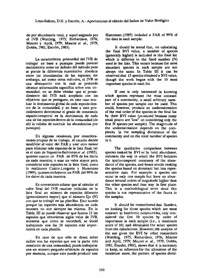
Es conveniente aclarar que al calcular el valor final del IVB resultan incluidas en la lista final un número de especies diferente (generalmente mayor) que el número fijo (N) con que se trabajó en las planillas. Esto sucede porque las especies más abundantes en cada muestra no son siempre las mismas. En la Tabla III se puede observar que fueron 15 las especies que obtuvieron algún valor de IVB, mientras que como se recordar& se inició trabajando con las 10 especies más importantes en cada planilla.

En caso de que s610 se desea saber miles son las especies que son la parte mas constante de una comunidad, puede trabajarse con un número pequeño arbitrario de especies por muestra, aunque esto puede producir una

HammaM (1989) included a PAR of 99% of the data in each sample.

It should be noted that, on calculating the final BVI value, a number of species (general@ higher) is included in the fmal list which is different to the fixed number (N) used in the lists. This occurs because the most abundant species in each sample are not always the same. In Table III it can be observed that 15 species obtained a BVI value, though the work began with the 10 most important species in each list.

If one is only interested in knowing which species represent the most constant part of a community, a small arbitrary number of species per sample can be used. This could, however, produce an underestimation of the real order of the species in the final list by their BVI value (producecl because many small points are “lost” on considering only the fust N species per sample). The magnitude of the underestimation depends on the com- plexity in the sampling dominance of the community and on the total number of species in it.

The qualitative comparison between species ranked by BVI or by total abundance, indicates the way in which the BVI balances the spatiotemporal constancy of the abundance of the species, and hence avoids ranking the species based on dominant but less repre sentative data. For example: a species can occur in only one sample but have an abundance several orders of magnitude higher than the other species and thus stay in fxst place. This is a methodological error since this species is not representative of the fauna in the samples.

It should be remembered that Sanders, on looking for those species which are most constant in benthonic communities, only considered the fust 10 species by order of importance in each sample (i.e., a maximum score of 10) and eliminated the other species from the calculations. However, the analysis of the use given the BVI by other researchers (Wattling, 1975; Richardson, 1976; Maurer and April, 1979; Maurer et al., 1979; Dobbs, 1981; Escofet, 1983), shows that it is necessary to keep, as referencefor the allocation of the maximum score, the pattem of species domi-

I-aya-Salinas, D.H. y Escofet, A.- Aportaciones al calculo del Indice de Valor Biológico

110

Laya-Salinas, D.H. y Escofet, A.- Aportaciones al c&lculo del Indice de Valor Biológico

sub-estimaci6n del orden real de las especies en la lista final por su valor de IVB (produ- cido porque muchos puntajes pequeños se “pierden” al considerarse ~510 las primeras N especies por muestra). .La magnitud de la sub-estimación depende de la complejidad en la dominancia muestral de la comunidad y del número total de especies en ella.

nance in the samples. It should be stressed that it is not the same to say that 10 species are representative of a total of 20 speciw as to say that they are of a total of 100 species. This is the same as assuming that the dominance found in the samples is not an important factor in ranking the representativity of the species.

El orden de importancia de las especies asignado en base al IVB, al ser comparado cualitativamente con el orden de importancia asignado por abundancia total, resalta el modo en que el IVB balancea la constancia espa- ckkternporal de la abundancia de las especies, y de este modo evita la ordenación de las especies en base a datos puntuales dominantes pero poco representativos. Por ejemplo: una especie puede estar en una sola muestra pero tener una abundancia de varios órdenes de magnitud mayor a las demaS especies y por esto quedar en el primer lugar, lo cual es un error metodol6gico debido a que esa especie no es representativa del conjunto faunfstico en las muestras.

Ascanbeseenfromthedata usedasan example in this study, the total number of species is modest and the community structure very simple (transect of a sandy beach). N = 10 speciea was cmsidered in each sample and that was enough to accumulate 95% of the individuals in each sample.

Antes de seguir adelante debe recordarse que Sanders, por estar buscando aquellas especies que son la parte mas constante de la comunidad bentónica, s610 consideró a las 10 primeras especies por orden de importancia en cada muestra (0 sea, un puntaje mzlximo de 10) y eliminó a las demás especies de los c4lculos. Sin embargo, al analizar el uso del IVB por otros investigadores (Wattling, 1975; Richardson, 1976; Maurer y April, 1979, Maurer et ai., 1979, Dobbs, 1981; Escofet, 1983), sobresale el hecho de que es necesario conservar, como punto de referencia para asignar el valor del puntaje máximo, al patrón de dominancia de las especies en las muestras Con esto se desea recalcar que no es lo mismo decir que 10 especies son representativas de un total de 20 especies a decir que lo son de un total de 100 especies, pues esto equivale precisamente a suponer que ‘la domman& encontrada en las muestras no es un factor importante en la ordenación de la representa- tividad de las especies.

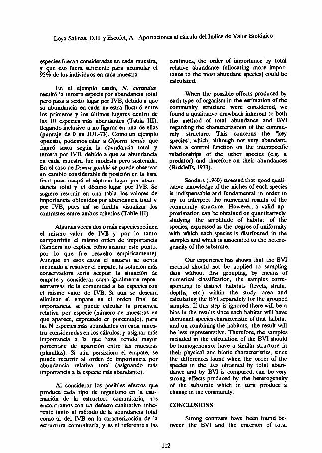
In the example used, N. cinntulus was the third species in order of total abundance but moved to sixth place by BVI, because its abundarme in each sample fluctuated between the fm and last places within the 10 most abundant species (Table III) and it did not even fwre in one of them (a value of 0 in JUL-73). On the other hand, G@em tenti was sixth according to total abundance and third by BVI, because its abundance in each sample was modest but steady. In the case of Lkmm gaddii, a considerable change of place in the final list can be observed since it occupied seventh place by total abundance and tenth place by BVI. The values of importance obtained by total abundance and BVI should be summarized in a table, making it easier to visualize the contrast between both criteria (Table III).

Como puede apreciarse en los datos usados como ejemplo para este trabajo, el número total de especies es modesto y la estructura comunitaria muy sencilla (transecto en una playa arenosa), produciendo que N = 10

Occasionally, two or more species will have the same BVI value and so will share the same order of importance (!Ianders did not clariQ this point and it was thereforeresolved empirically). Even though the user may be inclined to resolve the tie in these cases, the most conservative solution would be to accept the tie situation and consider the specieswith the same BVI value as equally repreaentative of the community. If the user still wants to eliminate the tie in the fmal order of importance, the relative presenceper species can be calculated (number of samples, expressed in percentage, in which it appears) for the N most abundant species in each sample consi& ered in the calculations, assi@g more importance to the one which appears most frequently in the samples (lists). If the tle

111


especies fueran consideradas en cada muestra, y que eso fuera suficiente para acumular el 95% de los individuos en cada muestra.

continues, the order of importance by total relative abundance (allocating more importance to the most abundant species) could be calculated.

En el ejemplo usado, N. cimtulus resultó la tercera especie por abundancia total pero pasa a sexto lugar por IVB, debido a que su abundancia en cada muestra fluctuó entre los primeros y los últimos lugares dentro de las 10 especies más abundantes (Tabla III), llegando inclusive a no fwrar en una de ellas (puntaje de 0 en JUL-73). Como un ejemplo opuesto, podemos citar a Glycem tenuis que fwró sexta según la abundancia total y tercera por IVB, debido a que su abundancia en cada muestra fue modesta pero sostenida. En el caw de Lhar gouldii se puede observar un cambio considerable de posición en la lista final pues ocupó el séptimo lugar por abundancia total y el décimo lugar por IVB. Se sugiere resumir en una tabla los valores de importancia obtenidos por abundancia total y por IVB, pues así se facilita visualizar los contrastes entre ambos criterios (Tabla III).

When the possible effects produced by each type of organism in the estimation of the community structure were considered, we found a qualitative drawback inherent to both the method of total abundance and BVI regarding the characterization of the community struuure. This concems the “key species”, which, although not very abundar& have a control function on the interspecilic relationships of the other species (e.g. a predator) and therefore on their abundances (Bickleffs, 1973).

Algunas veces dos o más especies reúnen el mismo valor de IVB y por lo tanto compartir&n el mismo orden de importancia (Sanders no explica calmo aclarar este punto, por lo que fue resuelto empiricamente). Aunque en esos casos el usuario se sienta inclinado a resolver el empate, la solución más conservadora sería aceptar la situación de empate y considerar como igualmente repre sentativas de la comunidad a las especies con el mismo valor de IVB. Si aún se deseara eliminar el empate en el orden final de importancia, se puede calcular la presencia relativa por especie (número de muestras en que aparece, expresado en porcentaje), para las N especies más abundantes en cada muestra consideradas en los c&ulos, y asignar mas importancia a la que haya tenido mayor porcentaje de aparición entre las muestras (planillas). Si aún persistiera el empate, se puede recurrir al orden de importancia por abundancia relativa total (asignando más importancia a la especie mas abundante).

Sanders (1960) stressed that good qualitative knowledge of the niches of each species is indispensable and fundamental in order to try to interpret the numerical results of the community structure. However, a valid ap proximation can be obtained on quantitatively studying the amplitude of habitat of the species, expressed as the degree of uniformity with which each species is distributed in the samples and which is associated to the heterogeneity of the substrate.

Al considerar los posibles efectos que produce cada tipo de organismo en la esti- mación de la estructura comunitaria, nos encontramos con un defecto cualitativo inhe rente tanto al método de la abundancia total como al del IVB en la caracterización de la estructura comunitaria, y es el referente a las

Our experience has shown that the BVI method should not be applied to sampling data without fust grouping, by means of numerical classilkation, the samples corre sponding to distinct habitats (levels, strata, depths, etc.) within the study area and calculating the BVI separately for the grouped samples. If this step is ignored there will be a bias in the results since each habitat will have dominant species characteristic of that habitat and on combining the habitats, the re-sult will be less representative. Therefore, the samples included in the calculation of the BVI should be homogenousor have a similar structure in their physical and biotic characteristics, since the differences found when the order of the species in the lists obtained by total abundance and by BVI is compared, can be very strong effects produced by the heterogeneity of the substrate which in tum produce a change in the community.

CONCLUSIONS

Strong contra& have been found between the BVI and the criterion of total

112

“especies clave”, que son aquellas especies que aunque poco abundantes tienen una función de control sobre las relaciones interespecilicas de las demás especies (v.g.: un depredador) y por lo tanto sobre sus abundancias (Rickleffs, 1973).

Sanders (1960) recalca que un buen conocimiento cualitativo del nicho de cada especie es indispensable y fundamental para tratar de interpretar los resultados numéricos de la estructura comunitaria. Sin embargo, una aproximación válida puede obtenerse al investigar cuantitativamente la amplitud de habitat de las especies, expresada como el grado de uniformidad con que se distribuye cada una de las especies en las muestras, y que esta asociada a la heterogeneidad del sustrato.

Parte de nuestra experiencia respecto al uso correcto del IVB, consiste en que este no debe de ser aplicado en datos de muestreos sin antes agrupar por medio de clasificación numérica a las muestras que corresponden a distintos habitats (niveles, estratos, profundi- dades, etc.) dentro del &rea de estudio y calcular los IVB por separado para las muestras agrupadas. El ignorar este paso incorpora un sesgo en los resultados debido a que ca& habitat tendrá especies dominantes caracteris ticas de ese habitat y al combinar los habitats el resultado pasa a ser menos representativo; por lo tanto el criterio a seguir es tratar de que las muestras incluidas en el calculo del IVB tengan una homogeneidad o semejanza estructural en sus características físicas y bióticas, pues las diferencias captadas cuando se compara el orden de las especies en las listas obtenidas por abundancia total y por IVB, pueden ser efectos muy fuertes producidos por la heterogeneidad del sustrato, que a su vez producen un cambio en la comunidad.

CONCLUSIONES

Se han encontrado fuertes contrastes entre el IVB y el criterio de la abundancia total, debido a la manera en que el IVB transforma las abundancias en puntajes, y de este modo asigna mayor peso en los c&lculos a la constancia espacio-temporal de las abundancias, que a alguna abundancia puntual grande. El IVB es un fndice que ha tenido buena aceptación en la ecología marina. Por su estructura, este trabajo ayudará bastante a

abundance, due to the manner in which the BVI transforms the abundances into points and in this way assigns more weight to the calculations of the spatio-temporal constancy of the abundances than to some large single abundance. The BVI has been well accepted in marine ecology. Because of its structure, this work will greatly help orientate BVI users, using it as referente for the details of the proposed algorithm. However, the characteris tics of the BVI in relation to other indices which also cany out the same function should continue to be studied.

ACKNOWLEDCEMENlS

The use of the PRIME-750 computer of the Computing Centre of CICBSE is acknowl- edged. We thank Gregory Hammann and Jorge RosalesC. for their revisions of the tart. The graphic work was done by Jose Marfa Domínguez.

English translation by Christine Harris.

orientar a los usuarios del IVB, usandolo como referencia para los detalles del algoritmo propuesto; sin embargo, deben seguirse in- vestigando las caracteristicas del IVB con respecto a otros indices que realicen la misma función de ordenación.

AGRADECIMIENTOS

Al Centro de Computo Electrónico del CICESE por el uso de sus computadoras PRIME-750 durante la implementación de los programas. Se agrad& a Gregory Hammann y a Jorge Rosales C. por sus revisiones del texto. El trabajo grrltico fue realizado por Jose Maria Dominguex.

LITERATURA CITADA

Andrewartha, H.G. and Birch, L.C. (1982). Empirical examples of the numbers of animals in natural populations. In: Selections from the Distniution and Abundance of Animals. The Univ. of Chicago Press, Chicago, 275 pp.

Atilano-Silva, HM. (1987). Composición y estructura de la comunidad del fitoplancton silíceo en el Golfo de California en mamo de


113


1983. Tesis de Licenciatura, Facultad de Ciencias Marinas, UABC, 161 pp.

Beltrán-Félix, J.L. (1984). Distniución, abundancia y diversidad de peces adultos en el Estero de Punta Banda, Ensenada, Baja California. Tesis de Maestria en Ciencias, CICESE, 89 pp.

Escofet, A. (1983). Community ecology of a sandy beach from Patagonia (Argentina, South America). M.S. Thesis, Univ. of Wash- ington, 122 pp.

Fager, E.W. (1957). Determinationand analysis of recurrent groups. Ecology, 38: 586-595.

Beltrán-Feliz, J.L., Hammann, M.G., Chagoya Guzmán, A. y Alvarez Borrego, S. (1986). Ictiofauna del Estero de Punta Banda, Ense nada Baja California, México, antes de una operación de dragado. Ciencias Marinas, 12(l): 79-92.

Field, J.G., Claike, K.R. and Warwick, RM. (1982). A practica1 strategy for analysing multispecies distribution pattems. Mar. Ecol. Progr. Ser., 8: 37-52.

Boe-sch, D.F. (1977). Application of numerical classification in ecological investigations of water pollution. Virginia Inst. Mar. Sci., Special Scientifc Report Rn,113 pp.

Grijalva-Chan, J.M. (1985). Distribución y abundancia de huevos y larvas de peces en la Bahía de Todos Santos, B.C., M&ico. Tesis de Licenciatura, Esc. Sup. Ciencias Marinas, UABC, 114 pp.

Calderón-Aguilera, L.E. (1984). Ecologfa de las comunidades de poliquetos bent6nicos (Annelida: Polychaeta) de la Bahfa de San Quintín, Baja California, Tesis de Maestrla en Ciencias, CICESE, 151 pp.

Guille, A. (1971). Bionomia benthique du plateau continental de la cote catalane fran- caise. VI: DOMC% autoecologiques (macro- fauna). Vie et Milieu, B 22(3): 469-527.

Castro-Longo@ E. y Hammann, M.G. (1989). Biomasa y composición general de la comunidad de zooplancton de la Bahfa de Todos Santos, B.C., M&ico, durante el evento de El Niño 1982-1983. Ciencias Marinas, 15(4): l-20.

Hernández-Alfonso, I., Hammann, M.G. y Rosales-Casián, JA. (1987). Zooplancton suprabentónico de la Balúa de Todos Santos, Baja California, M&dco, durante otoño 1986 e invierno 1987. Ciencias Marinas, 13(4): 53-68.

Clifford, H.T. and Stephenson, W. (1975). An Introduction to Numerical Classification. Aca- demic Pr* 229 pp.

Jim&mz-Perez, L.C. (1987). Caracteristicas est~Uuraks del zooplancton del Golfo de California durante el fenómeno El Niño (19821983). Tesis de Maestría en Ciencias, CICESE, 119 pp.

Cole, L.C. (1949). The measurement of inter- specific association. Ecology, 30: 411-424.

Conover, WJ. (1980). Practical Nonparamet- ric Statistics, 2nd. ed., Tatas Tech. Univ., John Wiley and Sons, New York, 493 pp.

Ludwig, JA. and Reynolds, J.F. (1988). Ecological community data. In: Statistical Ecology. A Primer on Methods and Comput- ing. John Wiley & Sons, New York, 337 pp.

Maurer, D. and April, G. (1979). Intertidal benthic invertebrates and sediment stability at the mouth of Delaware Bay. Int. Rev. ges. Hydrobiol., 64(3): 379403.

Dobbs, F.C. (1981). Community ecology of a shallow subtidal sand flat, with emphasis on sediment reworking by Clpnenella tonpata (Polychaeta: Maldanidae). M.S. Thesis, Univ. of CoMeuicut, 110 pp.

Maurer, D., Leathem, W., Kinner, P. and Tinsman, J. (1979). Seasonal fluctuations in coastal benthic invertebrate assemblages. Est. Coast. Mar. Science, 8: 181-193.

Elias, R. (1987). Estudio inventarial y ecológi- co del macrobentos de la Bahla Blanca. Tesis de Doctor en Ciencias Naturales, Instituto Argentino de oceanografíq 255 pp.

McCloskey, L.R. (1970). The dynamics of the community associated with a marine sclerao tinian coral. Int. Rev. ges, Hydrobiol., 55(l): 13-81.

114

Laya-Salinas, D.H. y Escofet, A.- Aportaciones al calculo del Indice de Valor Biol6gico

Milstein, A., Juanito, M. y Olazarri, J. (1976). Algunas asociaciones bentónicas frente a las costas de Rocha, Uruguay. Resultados de la Campaña del R/V “Hero”, 723A. Com. Soc. Malac. Uruguay, 6(30): 143-l&&

PamplonaSalazar, M.H. (1977). ES~NUU~ de una comunidad de invertebrados en una playa arenosa de la Bahía de Todos Santos, B.C. Tesis de Licenciatura, UABC, 46 pp.

Pearson, T.H. (1975). The benthic ecology of Lock Linnhe and Loch Eil, a sea-loch system on the west coast of Scotland. IV. Changes in the benthic fauna attniutable to organic enrichment. J. exp. mar. Bio. Ecol., 20: 141.

Pickett, S.TA. and White, P.S. (1985). Dis turbancemediated coexistence of species. In: The Ecology of Natural Disturbance and Patch Dynamics. Academic Press, Inc., San Diego, 472 pp.

Richardson, M.D. (1976). The classitkation and struuure of marine macrobenthic assemblages at Arthur Harbor, Anvers Island, Antarctica. Ph.D. Thesis, OregonState Univ., 142 pp.

Rickleffs, R.E. (1973). Community ecology. In: The Economy of Nature. 2nd. edition, Chiron Press, Inc., New York, 510 pp.

RuizCampos, G. (1986). Estructura trófica, composición y dinamica de la comunidad íctica de las pozas de marea durante otoñ&n- viemo en la playa rocosa de Granada Cove, Bahía de Todos Santos, B.C., Mkxico. Tesis de Maestrfa en Ciencias, CICESE, 120 pp.

Sanders, H.L. (1960). Benthic studies in Buzzard Bay. III. The structure of the soft-bottom community. Limnol. Oceanogr., 5: 138-153.

Sanders, H.L., Grassle, J.F., Hampson, G.R. Morse, L.S., Gardner-Price, S. and Jones, C.C. (1980). Anatomy of an oil spill: long-term effects from the grounding of the barge Florida off West Falmouth, Mas sachusetts. J. Mar. Res., 38(2): 265-381.

Siqueiro.+Beltrones, DA., Ibarra-Obando, S.E. y Laya-Salinas, D.H. (1985). Una aproxi- mación a la estructura floristica de las diatomeas epifitas de Zostem maha y sus variaciones temporales, en Bahla Falsa, San Quintín, B.C. Ciencias Marinas, ll(3): 69-88.

Smith, R.W. (1976). Numerical Analysis of Ecological Survey Data. Ph.D. Thesis, Univ. South. Calif., 401 pp.

Stephens, J. and Zerba, K.E. (1981). Factors affecting fti diversity on a temperate reef. Env. Biol. Fish., 6(l): 111-121.

Wattlin& L. (1975). Analysis of struuural variations in a shallow estuarine deposit-feed- ing community. J. Exp. Mar. Biol. Ecol., 19: 275-313.

Whiting, M.C. and Mdntire, C.D. 1985. An investigation of distniutional pattems in the diatom flora of Netarts Bay, Oregon, by corresponderme analysis. J. Phycol., 21: 655-661.

Zarkanel@ AJ. and Kattoulas, M.E. (1982). The ecology of benthos in the Gulf of Ther- maikos, Greece. Mar. Biol., 3(l): 21-39.

115

Aportaciones al cálculo del ÍNDICE DE VALOR BIOLÓGICO ...€¦ · Loya-Salinas, D.H. y Escofet,...

Documents

Transcript of Aportaciones al cálculo del ÍNDICE DE VALOR BIOLÓGICO ...€¦ · Loya-Salinas, D.H. y Escofet,...