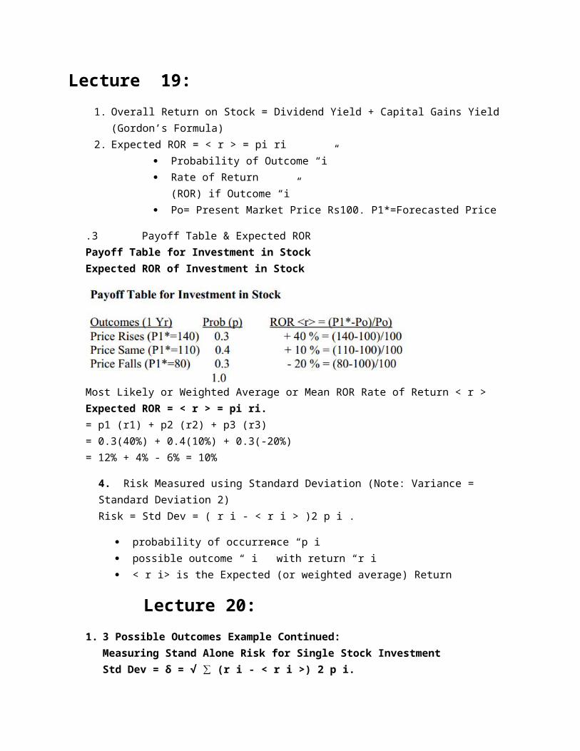
Lecture 19:1. Overall Return on Stock = Dividend Yield + Capital Gains Yield (Gordon’s

Formula)2. Expected ROR = < r > = pi ri

Probability of Outcome “i” Rate of Return

(ROR) if Outcome “i” Po= Present Market Price Rs100. P1*=Forecasted Price

.3 Payoff Table & Expected RORPayoff Table for Investment in StockExpected ROR of Investment in Stock

Most Likely or Weighted Average or Mean ROR Rate of Return < r >Expected ROR = < r > = pi ri.= p1 (r1) + p2 (r2) + p3 (r3)= 0.3(40%) + 0.4(10%) + 0.3(-20%)= 12% + 4% - 6% = 10%

4. Risk Measured using Standard Deviation (Note: Variance = Standard Deviation 2)Risk = Std Dev = ( r i - < r i > )2 p i .

probability of occurrence “p i possible outcome “ i ” with return “r i < r i> is the Expected (or weighted average) Return

Lecture 20:1. 3 Possible Outcomes Example Continued:

Measuring Stand Alone Risk for Single Stock InvestmentStd Dev = δ = √ ∑ (r i - < r i >) 2 p i.= (∑(r i - < r i >) 2 p i.)) 0.5.= {[(40-10)2 (0.3)] + [(10-10)2 (0.4)] + [(-20-10)2 (0.3)] } 0.5 .= {270 + 0 + 270} 0.5 = {Var} 0.5.= {540} 0.5 = 23.24How do we interpret this Result for Risk?

2.

3.(Coefficient of Variation )CV = Standard Deviation / Expected Return.

CV = σ/ < r >

Compare the CV’s of the Projects:CV T-bill = 5% / 10% = 0.5CV Project C = 30% / 30% = 1.0Choose the Project with the Lowest CV. Choose the T-Bill because it carries the lowest Risk per unit Return.

Lecture 21:

1. Future Rate of Return will lie within -1σ and +1 σ range2. < r > = Exp or Weighted Avg ROR = pi ri3. Total Stock Risk = Diversifiable Risk + Market Risk4. Portfolio’s Expected Rate of Return: ( rP ).

rP * = r1 x1 + r2 x2 + r3 x3 + … + rn xn

5. 2 Stock” Investment Portfolio RiskPortfolio Risk is generally not the weighted average risk of the Individual

Investments. In fact, it isusually lessStock (Investment) Portfolio Risk Formula:p = √ XA2 σ A 2 +XB2 σ B 2 + 2 (XA XB σ A σ B AB)

XA is Investment A’s weight in the total value of the Portfolio σ A is Investment A’s Individual Risk (or standard deviation) O. AB is the Correlation Coefficient

6. Total Stock Risk = Diversifiable Risk + Market Risk

8.

Lecture 22:

7. Total Stock Risk = Diversifiable + Market Risk8. If Ro = 0 then Investments are Uncorrelated9. If Ro = + 1.0 then Investments are Perfectly Positively Correlated

and this means thatDiversification does not reduce Risk.

10. If Ro = - 1.0, it means that Investments are Perfectly Negatively Correlated and the Returns (or Pricesor Values) of the 2 Investments move in Exactly Opposite directions.

11.

12. rP * = xA rA + xB rB + xC rC (3 Stocks)

Lecture 23:1. Total Stock Return = Dividend Yield + Capital Gain Yield2. Portfolio risk is on X- axis and the portfolio

return on Y- axis.3. capital market line (CML)

CML Equation: rP* = rRF + [(rM - rRF) / σM] σP

rRF= risk free rate of returnrM = expected rate of return for the market of all possible stockσM = risk of the marketσP = risk of stock portfolio

Lecture 24:4. Share A’s Beta = +2.0 then that Share is Twice as risky (or volatile)

as the KSE Market5. Share B’s Beta = +1.0 then that Share is Exactly as risky (or volatile) as the

KSE Market6. If Share C’s Beta = +0.5 then that Share is only Half as risky (or volatile) as

the KSE Market7. The Beta of most Stocks ranges between + 0.5 and + 1.58. The Average Beta for All Stocks = Beta of Market = + 1.0 Always.

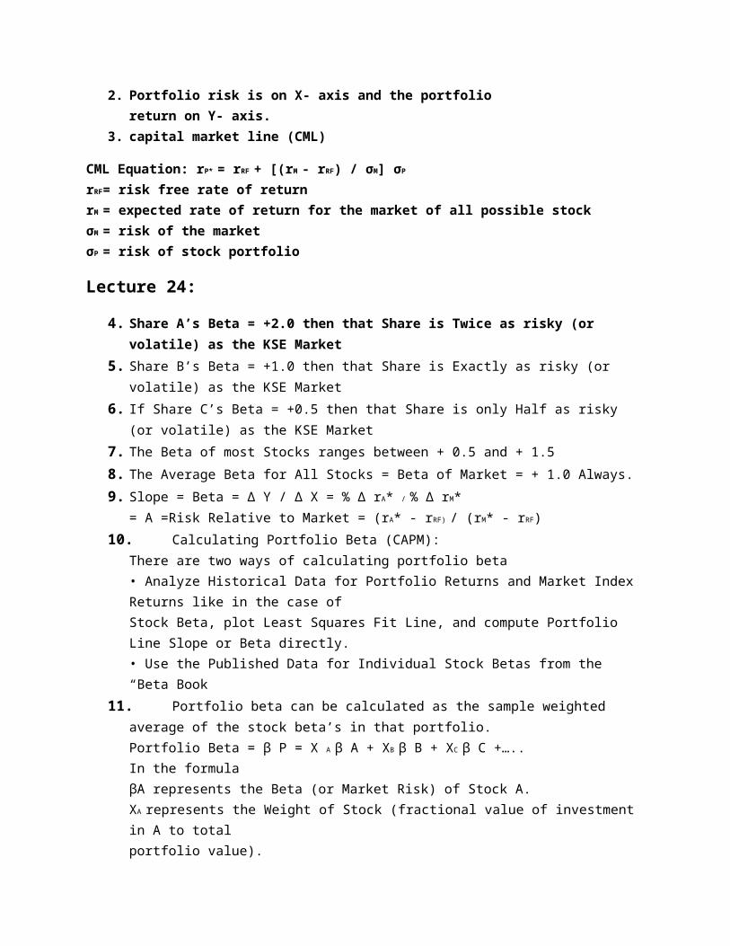
9. Slope = Beta = Δ Y / Δ X = % Δ rA* / % Δ rM*= A =Risk Relative to Market = (rA* - rRF) / (rM* - rRF)

10. Calculating Portfolio Beta (CAPM):There are two ways of calculating portfolio beta• Analyze Historical Data for Portfolio Returns and Market Index Returns like in the case ofStock Beta, plot Least Squares Fit Line, and compute Portfolio Line Slope or Beta directly.• Use the Published Data for Individual Stock Betas from the “Beta Book

11. Portfolio beta can be calculated as the sample weighted average of the stock beta’s in that portfolio.Portfolio Beta = β P = X A β A + XB β B + XC β C +…..In the formulaβA represents the Beta (or Market Risk) of Stock A.XA represents the Weight of Stock (fractional value of investment in A to totalportfolio value).

12.

13.

14.

Required ROR (r):

Total Rate of Return (ROR) for Single Stock = Dividend Yield + Capital Gain

. GORDON’S FORMULA FOR COMMON STOCK PRICING OR VALUATION USES REQUIRED RETURN r = DIV/Po + g.

15. In Efficient Markets, Price of Stocks is based on Market Risk (or Beta)

16. Security Market line SML

SML is straight line relationship stock A is directly proportional to Beta risk for that stock A

17. SML Linear Equation for the Required Return of any Stock A:rA = rRF + (rM - rRF ) β A .

In the above equation rA = Return that Investors Require from Investment in Stock A.

rRF = Risk Free Rate of Return (ie. T-Bill ROR). rM = Return that Investors Require from Investment in an Average Stock (or

the Market Portfolio of All

Stocks where β M = + 1.0 always). β A = Beta for Stock A. (rM - rRF )

β A = Risk Premium or Additional Return in Excess of Risk Free ROR to compensate the Investor for the additional Risk.

Lecture 25:1.Beta Stock A = % Δ rA* / % Δ rM* = Slope of Regression Line. Regression

Line usesExperimental Data.

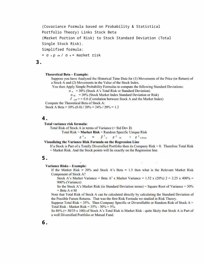
2.The formula that relates beta of the stock to the standard deviation is as followsBeta Stock A = Covariance of Stock A with Market / Variance of Market= σ A σ M ρ AM / σ 2 M

(Covariance Formula based on Probability & Statistical Portfolio Theory) Links Stock Beta(Market Portion of Risk) to Stock Standard Deviation (Total Single Stock Risk).Simplified formula:= σ A ρ AM / σ M = market risk

3.

4.

5.

6.

Lecture 26:1.

2. Required Rate of Return (rA)Risk premium=rA-rRF=30%-10%=20%.It is directly proportion to market risk of stock.3. slope of the SML line is = (rM-rRF)/ (betaM-0) = (rM-rRF)/1.4.

5.

NPV (and PV) Calculation which is the Heart of Investment Criteria and CapitalBudgeting uses required return (and NOT Expected ROR). This is why Share Pricing also usesRequired Rate of Return because Share Price was derived from the PV Equation for Dividend Cash Flows.

6. Asset Beta = Revenue Beta x [1 + PV (Fixed Costs)/PV (Assets)]

A Stock’s Beta or Risk Relative to the Market can change with time

7.

Lecture 27

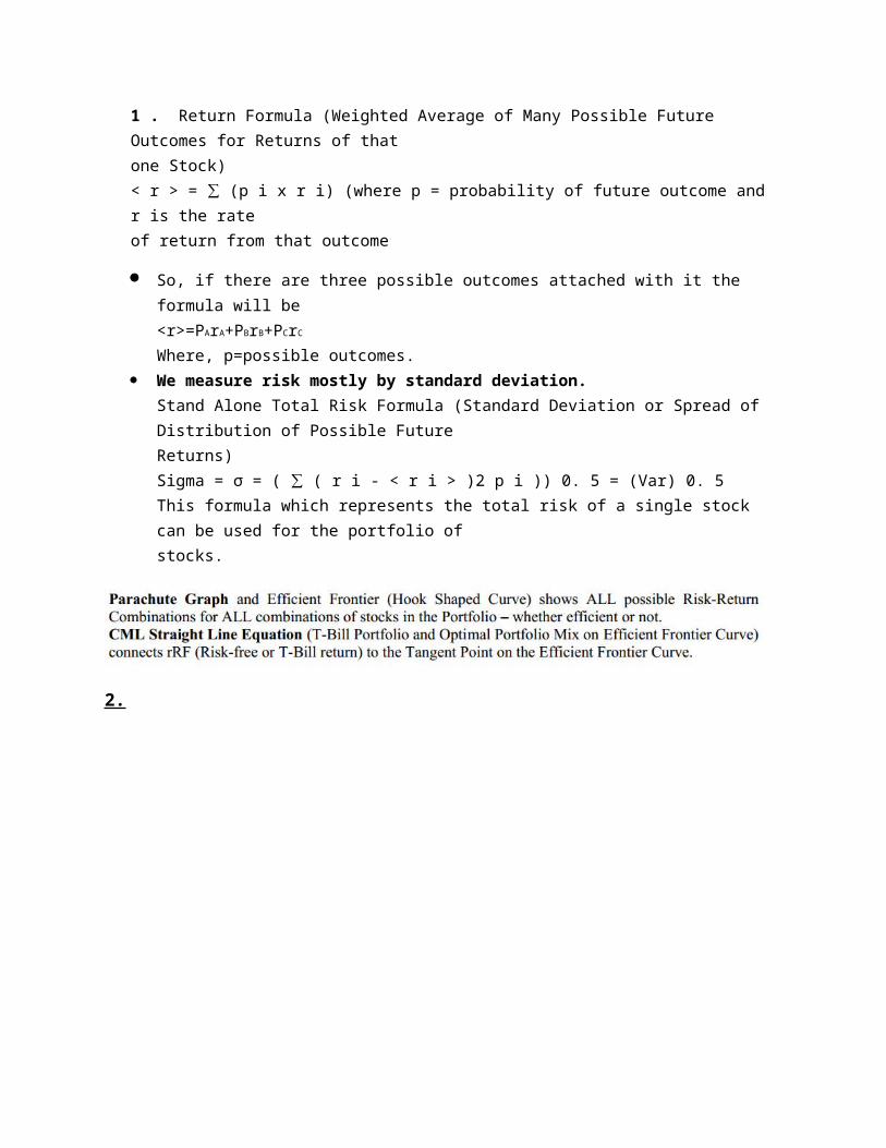
1 . Return Formula (Weighted Average of Many Possible Future Outcomes for Returns of thatone Stock)< r > = ∑ (p i x r i) (where p = probability of future outcome and r is the rateof return from that outcome

So, if there are three possible outcomes attached with it the formula will be<r>=PArA+PBrB+PCrC

Where, p=possible outcomes. We measure risk mostly by standard deviation.

Stand Alone Total Risk Formula (Standard Deviation or Spread of Distribution of Possible FutureReturns)Sigma = σ = ( ∑ ( r i - < r i > )2 p i )) 0. 5 = (Var) 0. 5This formula which represents the total risk of a single stock can be used for the portfolio ofstocks.

2.

3.

Total Risk or Standard Deviation (based on Spread or Range of Breadth of Possible RORoutcomes) = Unique + Market RiskSystematic (or Market or No diversifiable) Risk (= Beta A x Sigma M). Individual Risk relativeto Market or Industry.

Lecture 28

1.

2.

4. The Mixture or Proportion of Debt Capital and Equity Capital are known as the Capital Structure.This Financial Policy Decision is taken by the CEO, CFO, and Board of Directors

Capital Structure can Change With Time depending on Firm’s Financing needs and strategy.

Lecture 29 Cost of Debt Capital = rD Net proceeds = Market Price – Transaction Costs

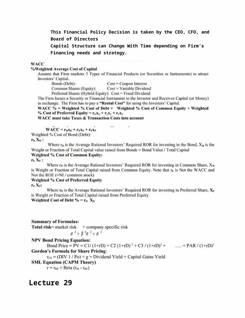
After Tax Cost of Debt = rD = rD* (1 - TC)Where TC is the Marginal Corporate Tax Rate on the Net Income of the Firm

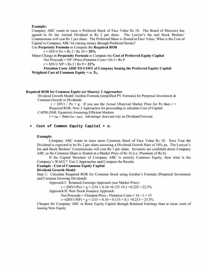
Cost of Common Equity Capital = rE

Lecture 30:

1. Issuing Debt (or Leverage)Advantages of Issuing Debt::

Limited fixed Interest payment - no share in profits Limited Life Interest Payment is an Expense i.e. Tax Deductible Can Improve (or Amplify) the Return on Equity (ROE)

Disadvantages: Debt adds to Company-specific Risk If company doesn’t pay Interest, it can be closed down

2. Issuing Equity (generally Common Equity or Ownership)Advantages of Issuing Equity:Not required to pay fixed regular Dividends

3. Firm’s Total Stand Alone Risk = Business + Financial4. Total Assets = Total Liabilities = Debt + Equity5. Operating Leverage (OL):

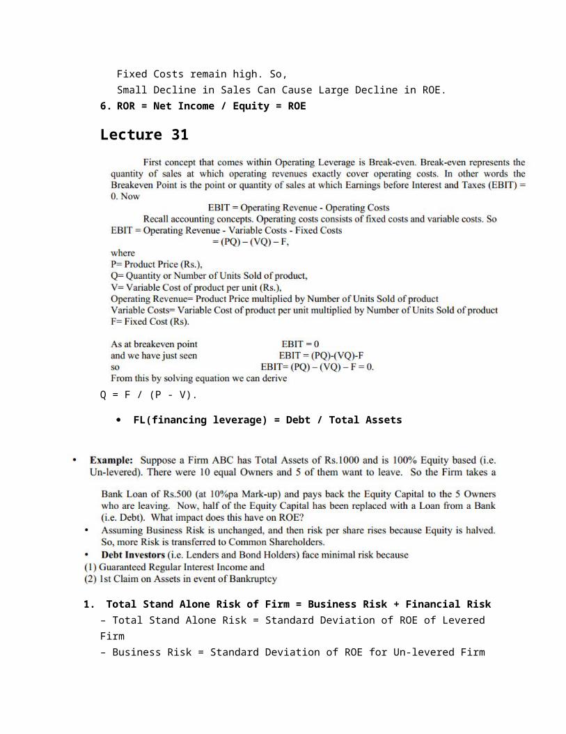
Formula = Fixed Costs / Total CostsConcept: High OL Increases Risk: Customer Demand Falls but Fixed Costs remain high. So,Small Decline in Sales Can Cause Large Decline in ROE.

6. ROR = Net Income / Equity = ROE

Lecture 31

Q = F / (P - V).

FL(financing leverage) = Debt / Total Assets

1. Total Stand Alone Risk of Firm = Business Risk + Financial Risk– Total Stand Alone Risk = Standard Deviation of ROE of Levered Firm– Business Risk = Standard Deviation of ROE for Un-levered Firm

2. Financial Leverage (FL) & Operating Leverage (OL):3. Return on Equity ( ROE)

Lecture 32:

Modigliani - Miller:• Fathers of Corporate Finance• “Cost of Capital, Corporate Finance and the Theory of Investment” Revolutionary ArticlePublished by Professors Modigliani & Miller in American Economic Review in June 1958.Won Nobel Prize.• “Pure M-M” (or Modigliani-Miller) Model - IDEAL CASE

Lecture 33Now we come to the cost of equity of levered firmrE,L =WACC + Debt/Equity (WACCL - rD,L)= 21% + 400/600 (21% - 13%)= 26.3%rE,L= (WACC - rD,L xD)/ xE

= (21% - 13% (400/1000)) / (600/1000)= 26.3%• Cost of Equity for Levered Firm= rE,L = Risk Free Interest Rate + Business Risk Premium + Financial Risk Premium.rE,L increases because required ROR for stock increased because of financial risk.

Traditionalists Formulas for Equity:E = Net Income (NI)/ Cost of Equity for levered firm (rE,L)Note that NI = EBIT - Interest - Tax = EBT – TaxNI = (EBIT - xD rD) (1 - Tc)rE,L = WACCU + xD (WACCU - rD ) (1 - Tc).• Traditionalists Formula for WACC:WACCL = xD rD (1 - Tc) + xE rE.(1-Tc) is the Tax Discount Factor.

Note: Value of firm = Debt + EquityxD = Debt /Value = Debt/ (Debt + Equity)xD + xE = 1V = Market Value of Firm D = Market Value of DebtE = Market Value of EquityxD = Fraction of Debt = A Measure of Leverage

Lecture 35:

Following formula has been used to calculate the WACC:WACCL = rD xD (1 - Tc) + rE xE.WACCL = 10%* (200/1059) (1 – 30%) + 22% * (859/1059).= 19.17%

NI Approach for Calculating Numerical value of WACC of Levered Firm – Example:• Starting Point for Calculating Numerical Value of WACC suing NI Approach is EBIT of Firm= Rs.100 and Corporate Tax Rate, Tc = 30%– If the Firm is 100% Equity (or Un-Levered) and rE = 20% then what is the WACCU ofUn-levered Firm?• Net Income = EBIT - Interest - Tax= 100 - 0 - 0.3(100)= Rs.70• Market Value of Un-levered Equity = Eu= NI / rE

= 70 / 0.2= Rs.350• Market Value of Un-levered Firm = Vu= Equity + Debt= 350 + 0= Rs.350• WACC u = rE,U

= 20%

– If the Firm takes Rs.100 Debt at 10% Interest or Mark-up then what is the WACCL ofLevered Firm?• Net Income (NI)= 100 - 10 %( 100) - Tax= 100 - 10 - 0.3(90)= Rs.63• Equity= NI / rE

= 63 / 0.2= Rs.315 (Major Assumption: No change in rE)• VL = Equity + Debt= 315 + 100= Rs.415. (Increasing Debt ADDS Value!)• WACCL= rD,L (1-Tc) xD + rE,LxE

= 0.1(1-0.3) (100/415) + 0.2(315/415)= 16.9%Point to note is that WACCL is lower than WACCU.• Sequence of Steps:(1) Calculate NI = EBIT - Interest - Tax(2) Calculate E = NI / rE

(3) Calculate VL = Equity + Debt(4) Calculate WACCL

Market Value of Levered Firm= VL = Vu + Tc D.

Market Value of Equity = E = VL – D WACCL = rD,L(1-Tc) xD + rE,LxE

WACCL =WACCU (1-Tc) xD

Lecture 36: FCC (Fixed Charge Coverage) = (EBIT - Lease Rental) / (Interest + Lease

Rental +Adjusted Sinking Fund Payment).

Lecture 37:• Payout Ratio= Annual Dividend Amount/ Net IncomeANDDividend per Share= Total Dividend Amount / Outstanding Number of Shares• There needs to be a tradeoff between Dividend Income & Capital Gains

1. Earnings, Cash flows, Capital Structure, and Capital Budgets fluctuate up anddown with time but Dividend Payouts should NOT change much – known as“Sticky Dividend Policy

2. Growth = g= Plough back x ROE= (1 – Dividend Payout) x ROE

Lecture 38

2nd example

3rd example

• Fundamental Share Value Formula:Share Price = Po = EPS x (P/E)

Lecture 39:• Generally Working Capital (Gross) = Current Assets– Current Assets = Inventory + Accounts Receivables + Cash + Marketable Securities +…(The mentioned items are four major items)

• Net Working Capital = Current Assets – Current Liabilities

= Assets – Liabilities = Equity1. Current Liabilities= Accounts Payables + Accruals + Short Term Loans + … (as well as other minoritems)

• “Fat Cat” or Relaxed Policy– It requires Large Amount of Current Assets not to loose any sales i.e. when a customerplaces order for a large amount, there is no shortage of inventory– Occurs when High sales driven by lot of credit facility to buyers

• “Lean & Mean” or Restricted Policy– Small Amount of Current Assets – It increases turnover and therefore Profits• Current Asset Turnover = Sales / Current Assets. Higher than 20.• Lowers Carrying Costs of Inventory

• “Lean & Mean” or Restricted Policy– Small Amount of Current Assets – It increases turnover and therefore Profits• Current Asset Turnover = Sales / Current Assets. Higher than 20.• Lowers Carrying Costs of Inventory

• Moderate Policy– In between the Fat Cat and Lean & Mean Policies

Total Capital = Market Value of Debt + Market Value of Equity DuPont Formula:

ROE= Profit Margin x Asset Turnover x Leverage Factor (or Equity Multiplier)

= (Net Income/Sales) x (Sales/Assets) x (Total Assets/Equity)= Net Income / Equity

Lecture 40:• Gordon’s Formula:Dividend policy issue of the company can be seen through Gordon’s Formula.

Po (Share Price) = DIV1 / (rE – g)= EPS x (DIV1/EPS) / (rE – (Pb x ROE)).DIV1 = Forecasted dividend in the next yearrE = Required rate of return on equityg = Growth rate in dividendsPb = Plough back ratio

If ROE < rE then firm is not generating enough return to meet shareholder requirements so itis better to payout the dividend.

If ROE > rE then firm is better off to Plough the Retained Earnings back into the businessand investing in Positive NPV Projects or the Firm’s core business. In this case, companyis generating higher return than the return shareholders require,

If ROE = rE then dividend payment has no impact on share price of the company.

3 Types of Inventories: Raw Material, Work in Process, Finished Goods EOQ (Economic Order Quantity) Shortfall in Inventories: interruptions in production and loss or sales

orders Surplus Inventories: high carrying costs, wastage, and depreciation JIT: Just in Time. Developed by Toyota. Supplies arrive just a few hours

before they areused. Inventory and Working Capital is minimized. Improves overall Efficiency.

Total Assets = Fixed + Permanent Current + Temporary Current.

Ya ALLAH sb ko pass kr de is semester k sb subjects me.AMEEN