AO-A127 OF HYDRAU C DREDGING OR CLAM SHELLS IN LAKE … · ao-a127 189 environmenta effects of...
156
AO-A127 189 ENVIRONMENTA EFFECTS OF HYDRAU C DREDGING OR CLAM SHELLS IN LAKE PONTC (U) LOUISIANA STATE UNIV BATON ROUGE COASTAL ECOLOGY LAB W B SIKORA ET AL. dUN 81 UNCLASSIFIED LSU-CL8-8DC2-9CO~ F/G 5/1 NL IIIIIIIIIIIIIu IEEIIIIIIIIEI EIIIIIIIIIIIIu EEIIIIIIIIIEI EIIIIIIIIIIIII IIIIIIEIIIEIIE
Transcript of AO-A127 OF HYDRAU C DREDGING OR CLAM SHELLS IN LAKE … · ao-a127 189 environmenta effects of...
AO-A127 189 ENVIRONMENTA EFFECTS OF HYDRAU C DREDGING OR CLAMSHELLS IN LAKE PONTC (U) LOUISIANA STATE UNIV BATONROUGE COASTAL ECOLOGY LAB W B SIKORA ET AL. dUN 81UNCLASSIFIED LSU-CL8-8DC2-9CO~ F/G 5/1 NL
IIIIIIIIIIIIIuIEEIIIIIIIIEIEIIIIIIIIIIIIuEEIIIIIIIIIEIEIIIIIIIIIIIIIIIIIIIEIIIEIIE

1.8
11111.25 1111 1.4 1.6
MICROCOPY RESOLUTION TEST CHARTI NATIONAL BUREAU OF STANDARDS-1963-A
kEnvironmental Effects of-- , !I
Hydraulic Dredging for Clem Shellsn Lake Pontchartrain, Louisiana
by
Walter B. SikoraJean Pantell Sikora
buD Anny McK. Prior
N June 1981
s44a-LI -. r#7
-'Al
'~ A I ~PA
A '-4.r~V -r~v
OF.4 4
7"~ a
:z IN'.
Prep ared for
C... U.S. Army Engineer District, New OrleansC:) Contract No. DACW29-79-C-00994
LL.. Coastal Ecology Laboratory, Center for Wetland Resources,
Louisiana State University, Baton Rouge, Louisiana 70803*Publication No. LSUI-CEL-81I- 18-
. 8304 07 025

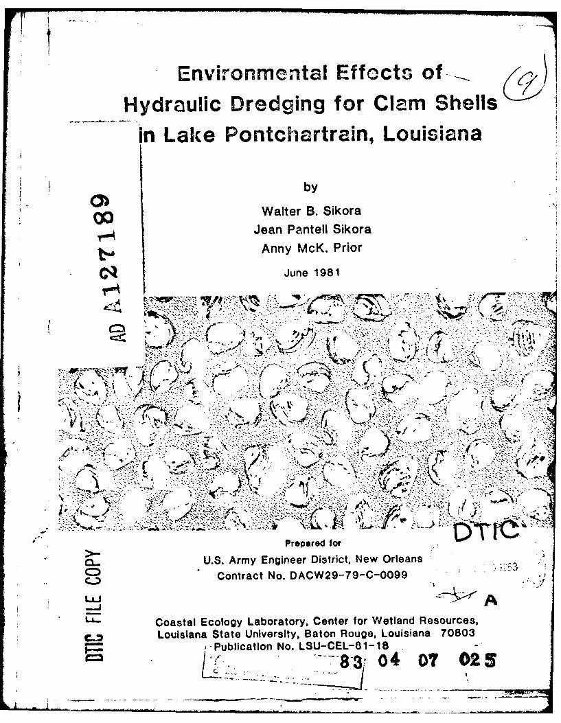
Environmental Effects ofHydraulic Dredging for Clam Shells
in Lake Pontchartrain, Louisiana
by
Walter B. SikoraJean Pantell Sikora
Anny McK. Prior
June 1981
Prepare forU.S. Army Engineer District, New Orleans
Contract No. DACW29-79-C-0099
Coastal Ecology Laboratory, Center for Wetland Resources,Louisiana State University, Baton Rouge, Louisiana 70803
Publication No. LSU-CEL-81-18.

PREFACE
This report presents the results of an investigation to determinethe recovery rates of benthic communities in Lake Pontchartrain, Louisiana,following hydraulic dredging for clam shells. This study was sponsoredby the New Orleans District of the U.S. Army Corps of Engineers (COE)under Contract No. DACW29-79-C-0099 to the Coastal Ecology Laboratory,Center for Wetland Resources, Louisiana State University, Baton Rouge,Louisiana.
The report was written and prepared by Walter B. Sikora and JeanPantell Sikora, except for the chemistry section, which was written byAnny McK. Prior, and the appended reports by David W. Roberts andLeonard H. Bahr, Jr., and by John W. Fleeger. This report has been desig-nated by the Coastal Ecology Laboratory as Contribution No. LSU-CEL-81-18.
Contracting Officer Representative of the COE was Frank J. Cali.John C. Weber, Sue R. Hawes, and Larry M. Hartzog assisted in review ofthe report.
The authors would like to acknowledge significant contributions byJ. Wilkins, laboratory manager, in the field and in the laboratory;K. Westphal, figures; J. Bagur, editorial suggestions; C. Lusk andB. Grayson, typing; E. Parton, assistance with data management; K. Westphal,N. Walker, H. Lindsay, R. Robertson, and C. Cardiff, assistance in fieldand laboratory; R. Wilson, boat captain and Dr. Richard W. Heard, taxonomicassistance. We would also like to acknowledge the cooperation of theLake Pontchartrain Shell Producers Association in several phases of thestudy and of the Greater New Orleans Expressway Commission for permittingthe experimental dredging at the study site within the restricted zoneof the Lake Pontchartrain Causeway.
i~
/4
ii

r-- Any mention of a commercial product or brand does not mean that theArmy Corps of Engineers or Louisiana State University endorses saidproduct or brand.
ii
I -- . .. . .. .-

TABLE OF CONTENTS
PAGE
PREFACE........................ .. ....... .... .. .. .. .. ......
LIST OF TABLES. .......... .................. v
LIST OF FIGURES .. .......... ................ vii
INTRODUCTION. ......... .....................
General Description of Lake Pontchartrain .. ............ 2Hydraulic Dredging for Clam Shells in Lake Pontchartrain ... 2Magnitude of Shell Dredging Operations. .. ............. 6Scope of Present Study .. ......... ............. 7
SHELL DREDGING AT THE EXPE2RIMENTAL SITE. .. .............. 8
Methods .. ................... ......... 11Results .. ................... ......... 11Discussion. .. ................. ......... 11
PHYSICAL EFFECTS OF SHELL DREDGING ON BOTTOM SEDIMENTS .. ...... 14
Methods .. ................... ......... 16Results .. ................... ......... 16Discussion. .. ................. ......... 16
THE EFFECTS OF SHELL DREDGING ON THE NUTRIENT ANDHEAVY METAL CHEMISTRY OF THE WATERS AND SEDIMENTSOF LAKE PONTCHARTRAIN. .. .................. .... 24
Introduction. .. ................. ........ 24Literature Review .. .................. ..... 24Materials and Methods. ........... ............ 30Results .. ................... ......... 34
Nutrients. .. ................... ...... 35Metals .. .................. ......... 48
Discussion. .. ................. ......... 70sumary .. ................. ............ 71conclusions .. ................... ....... 73
EFFECTS OF SHELL DREDGING ON THE BENTHIC FAUNAOF LAKE PONTCHARTRAIN. .. ................ ...... 74
Introduction. .. ................. ........ 74Methods .. .................. ........... 74Results .. .................. ........... 75Discussion. .. ................. ......... 93Sumery .. ................. ............ 99

CONTENTS PAGE
OVERVIEW . . . . . . . . . . . . . . . . . . . . . . . . . . . . . 100
CONCLUSIONS .... ....... ............................ ... 105
LITERATURE CITED .......... ......................... ... 106
APPENDIX A
SYSTEMATIC LIST OF BENTHIC MACROFAUNA; LAKE PONTCHARTRAINCONTROL AND EXPERIMENTAL DREDGING EFFECTS STATIONS ........ ... 114
APPENDIX B
MEIOFAUNA DATA ......... ......................... .... 115MACROFAUNA DATA ......... ........................ ... 119
APPENDIX C
BENTHIC COMMUNITY STRUCTURAL AND METABOLIC CHANGESALONG A TRANSECT THROUGH DREDGED AND UNDREDGED AREAS ........ ... 128I
APPENDIX D
EFFECT OF SHELL DREDGING ON LAKE PONTCHARTRAINMEIOBENTHIC COPEPODS ........ ...................... ... 139
iv
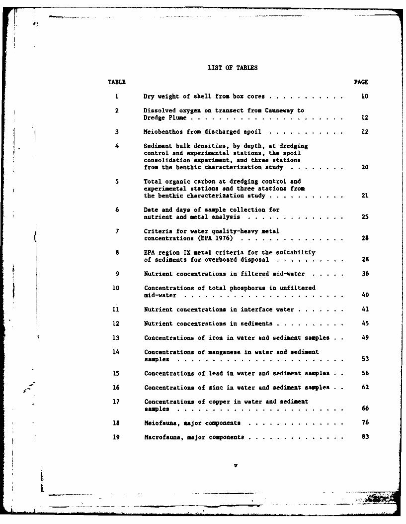
LIST OF TABLES
TABLE PAGE
1 Dry weight of shell from box cores .. ........... ... 10
2 Dissolved oxygen on transect from Causeway toDredge Plume ........ ...................... .... 12
3 Heiobenthos from discharged spoil .. ........... ... 12
4 Sediment bulk densities, by depth, at dredgingcontrol and experimental stations, the spoilconsolidation experiment, and three stationsfrom the benthic characterization study . ........ . 20
5 Total organic carbon at dredging control andexperimental stations and three stations fromthe benthic characterization study .. ........... ... 21
6 Date and days of sample collection fornutrient and metal analysis ....... .............. 25
7 Criteria for water quality-heavy metalconcentrations (EPA 1976) .... ............... ... 28
8 EPA region IX metal criteria for the suitabiltiyof sediments for overboard disposal . .......... ... 28
9 Nutrient concentrations in filtered mid-water ..... 36
10 Concentrations of total phosphorus in unfilteredmid-water ........ ....................... .... 40
11 Nutrient concentrations in interface water ....... ... 41
12 Nutrient concentrations in sediments .. .......... ... 45
13 Concentrations of iron in water and sediment samples . 49
14 Concentrations of manganese in water and sedimentsamples ........ ........................ .... 53
15 Concentrations of lead in water and sediment samples . 58
16 Concentrations of zinc in water and sediment samples . 62
17 Concentrations of copper in water and sedimentsamples ........ ........................ .... 66
18 Meiofauna, major components .... .............. ... 76
19 Nacrofauna, major components ....... .............. 83
V

TABLE PAGE
20 Macrofauna; species numbers, evenness and diversity ... 88
21 Hacrofauna; mean numbers and biomass per m2 andpercent numbers and biomass .. ........... .... 92
22 ?lacrofauna, numbers and biomass from the literature ... 97
Bi Meiofauna data .. ...................... 115
B2 Macrofauna data. .. ..................... 119
Dl Sumry of ANOVA statistics calculated on
harpacticoid copepod abundances .. ..............140
vi

LIST OF FIGURES
FIGURE PAGE
1 Lake Pontchartrain, La. showing major rivers,passes and inputs ......... ................... 3
2 Lake Pontchartrain, La. sampling stations andaverage isohalines for 1978 ....... .............. 4
3 Sediment grain size distribution for 1973........ 5
4 The Dredge Maurepas ......... .................. 9
5 Burial of sediment surface by dredge spoil atexperimental dredging station ...... ............. 15
6 Spoil consolidation experiment by depth through time . 18
7 Spoil consolidation experiment, drop in sedimentsurface through time ..... .................. .... 19
8 Ammonium nitrogen--midwater samples . .......... ... 37
9 Total inorganic nitrogen--filtered midwater samples . . 37
10 Orthophosphate--filtered midwater samples ....... . 38
11 Total phosphorus--unfiltered midwater samples .. ..... 38
12 Ammonium nitrogen--filtered interface water ...... . 42
13 Total inorganic nitrogen--filtered interface water . . . 42
14 Orthophosphate--filtered interface water .......... ... 44
15 Total phosphorus--interface particulate . ........ . 44
16 Total Kjeldahl nitrogen--interface particulate .. ..... 46
17 Total phosphorus--sediment .... ............... .... 46
18 Total Kjeldahl nitrogen--sediment .. ........... ... 47
19 Iron--filtered midwater ........ ................ 50
20 Iron--unfiltered midwater .... ............... ... 50
21 Iron--filtered interface water ...... ............. 51
22 Iron--interface particulate .... .............. ... 51
23 Iron--sediment ....... ..................... .... 54
vii

FIGURE PAGE
24 Manganese-- filtered midwater. .. .............. 54
25 Manganese--unfiltered midwater. .. ............. 55
26 Manganese-- filtered interface water .. ........... 55
27 Manganese-- interface particulate. .. ............ 56
28 Manganese-- sediment .. ................... 56
29 Lead--filtered midwater .. ................. 59
30 Lead--unfiltered midvater .. ................ 59
31 Lead--filtered interface water. .. ............. 60
32 Lead--interface particulate .. ............... 60
33 Lead--sediment .. ......... ............. 63
34 Zinc--filtered midwater .. ................. 63
35 Zinc--unfiltered midwater .. ................ 64
36 Zinc--filtered interface water. .. ............. 64
37 Zinc--interface particulate .. ............... 65
38 Zinc--sediment .. ......... ............. 65
39 Copper-- filtered midvater .. ................ 67
40 Copper--unfiltered midwater .. ............... 67
41 Copper--filtered interface water. .. ............ 68
42 Copper--interface particulate .. .............. 68
43 Copper--sediment .. ......... ............ 69
44 Meiofatzna abundance at control and experimentalsites .. ....... ....... ........ ... 78
45 Nematode abundance at control and experimental sites .81
46 Macrofauna abundance at control and experimentalsites. ......... .................. 82
47 Gastropod abundance at control and experimentalsites. .......... ................. 85
viii

FIGURE PAGE
48 Dendrogram illustrating classification ofcollections from study sites ... .............. .... 89
49 Ordination by principal coordinate analysis ofcollections from control and experimental sites . . .. 91
50 Log-normal plots of species abundances in geometricclasses ........ ........................ .... 96
Cl Location of transect and sampling stations ......... ... 129
C2 Organic carbon content and shell ratio of sediments 131
C3 Total community respiration as a function ofdistance from shore ...... .................. ... 131
C4 Total macrofauna and mieofauna biomass as a functionof distance from shore ..... ................. .... 133
C5 Biomass of the clams R. cuneata andM. pontchartrainensis ..... ................. ... 134
C6 Biomass of the hydrobiid snails P. protera andT. sphinctostoma ....... .................... ... 135
C7 Percent composition of meiofaunal biomass interms of dominant taxa and region in the lake .. ..... 137
iixii
.................- - - - -

INTRODUCTION
Hydraulic dredging is a common industrial activity in many coastalwaterbodies, including estuaries, and is often carried out on a largescale over long time periods. However, because different techniques areemployed to achieve different results, the effects of dredging operationsvary greatly. There is a need, therefore, to differentiate between thevarious types of dredging activities, which may be broadly classifiedinto two categories: channel dredging and mining. Channel and canaldredging can alter water circulation patterns, particularly by allowingintrusion of higher salinity water into normally low salinity environ-ments. Spoil piles from channel and canal dredging can redirect waterflow, altering normal water circulation and impeding normal mixing pro-cesses. These alterations can have rapid and long lasting effects, oftencompletely changing the ecology of large areas. Maintenance dredging,which often follows channel dredging and is undertaken to keep navigationchannels at prescribed depths, frequently involves the removal of mediumto coarse grained sediments in areas of high water flow. Results fromstudies of the effects of dredging in these systems are usually onlyapplicable to these same environments.
Mining by hydraulic dredging, although utilizing similar equipment,is usually carried out in open, semiprotected waterbodies with low waterflow, for the purpose of extracting buried shell deposits. Shell dredgingon the Gulf Coast is of two different types: oyster shell dredging andclam shell dredging. The two types of dredging could have quite differentenvironmental effects when viewed from the system level. Both types ofdredging by necessity involve the drastic disturbance of the bottomsediments and the indigenous benthic communities as they pass throughthe processing plant of the dredge. However, because oysters are reef-forming organisms, the shell resource is concentrated in clumps or bandsfrom less than a hundred meters to a kilometer wide and sometimes severalkilometers long, often buried 5 to 15 meters or more below the sedimentsurface. Often a deep hole 2 to 4 meters in depth remains after theoyster shell is extracted and the spoil sediment in the hole consolidates(Harper and Hopkins 1976). These holes can remain for many years, withresulting salinity and oxygen stratification. The overall result on asystem-wide basis is a potholed effect, with severe disturbance inconcentrated areas, yet with large, undisturbed areas. May (1973) andHopkins and McKinney (1976) present extensive literature reviews ofoyster shell dredging.
Clam shell dredging, on the other hand, presents a different set ofproblems. The shells of the brackish water clam Rangia cuneata aredeposited in shallow layers, 0.5 to 1 meter deep, blanketing the entirebottom of an estuary. The strategy for harvesting this resource is forthe dredges to move continuously at 5 to 8 kilometers per hour, constantlydredging a shallow trench 1 to 2 meters wide. Nearly 0.25 km2 per daywill pass through the processing plant of a single dredge, with a largerarea being affected by spoil. Several clam shell dredges working simul-taneously could affect an entire estuary in a matter of years.
General Description of Lake Pontchartrain
Lake Pontchartrain is a shallow (mean depth 3 m, maximum 5 m) body
of water of about 1630 km2 lying in the middle of a large, southeasternLouisiana estuarine complex (Figure 1). To the west is Lake Maurepas,connected to Pontchartrain by Pass Manchac; to the east, Pontchartrainis connected to the Mississippi Sound by The Rigolets Pass and to LakeBorgne by the Chef Menteur Pass. In the southeast, the man-made InnerHarbor Navigation Canal-Mississippi River Gulf Outlet complex connectsthe lake to the Gulf of Mexico. The majority of freshwater input intothe lake is from rivers emptying into the northwestern part of the lake;the Tickfaw River and the Amite-Comite River complex via Pass Manchac,and the Tangipahoa and Tchefuncte Rivers emptying directly into thelake. During flood years, Pontchartrain can receive Mississippi Riverwater via the Bonnet Carri Spillway and some Pearl River water via TheRigolets. During times of normal flow, higher salinity water enters theeastern portion of the lake via the passes.
Circulation within the lake has been shown to be primarily winddriven (GSRI 1972; Gael 1980), with current speeds of about 15-20 cm/sec(U.S. Army Corps of Engineers 1962). In addition, there is a diurnaltide with a mean amplitude of 11 cm (Outlaw 1979). The salinity regimeof the lake is quite low, with a mean of about 5 ppt, and it is horizon-tally stratified, with salinities highest in the eastern half and lowestin the western half. At times this gradient may reach 12 ppt. Theaverage isohalines for 1978 are shown in Figure 2. Also shown in Figure 2are the experimental and control dredging stations and the 13 stationsof the concurrent benthic characterization study. Variations in salinityand temperature in the vertical are small enough to be inconsequentialmost of the year, which indicates that the lake is vertically a well-mixed system. Lake temperatures show a generally isothermal pattern,the maximum spatial gradient being 4*C (Swenson 1980). Water temperaturegenerally follows air temperature, with a maximum water temperature ofabout 300C in August-September and a minimum of about 6*C in January-February. Clay and silty clay sediments predominate in the centralregion of the lake (Barrett 1976; Bahr, Sikora, and Sikora 1980) withsilty clay found at the dredging stations (Figure 3).
Because of the extensive area of the lake and hence its largefetch, wind-induced waves play an important role in the system. Swenson(1980) has shown that silty clay sediments can be resuspended by wind-induced waves of 0.75 m to 1.3 m in height, which occur with wind speedsof about 15 mph (6 m/sec). He has further shown (from Gael 1980) thatwinds of this speed or greater occur at least 15% of the time. Thus,one can conclude that the bottom of the lake is in motion at least 15%of the time because of natural causes.
Hydraulic Dredging for Clam Shells in Lake Pontchartrin
Hydraulic dredging for Ranlia shell in Lake Pontchartrain beganaround 1933 and has steadily intensified in the subsequent 48 years tothe present time. This trend can readily be seen from clam shell pro-duction estimates by the Louisiana Wild Life and Fisheries Comission,
2i

44it
"" fjA4.wS
44
SS
*414 .

4-4
004
r14 0
w4 0 .
0440LIw- is
5.1 64 4
u 6 N
4C
_____ __-. - - - -

I4V
As.. I.I
00'0

(1968), which range from 300,000 cubic yards statewide in the mid-thirtiesto 5,000,000 cubic yards, mainly from Lakes Pontchartrain and Haurepasin 1968. In recent times there have been two attempts at assessing theenvironmental effects of those operations in Lake Pontchartrain (Tarver1973, Gulf South Research Institute 1974). Neither of these efforts,however, were concerned with possible long-term effects, and both concludedthat short-term effects, particularly on the water column and on nektonicspecies, were negligible and transitory in nature. Any realistic evalua-tion of the effects of shell dredging would by necessity have to includethe long-term effects on the sediment structure and chemistry as well ason the benthic infauna, both macrofauna and meiofauna, which live in thesediments. Only then could projections be made to include the entirelake ecosystem through time.
Magnitude of Shell Dredging Operations
Before considering possible long-term effects of shell dredging onthe fauna or lake ecosystem as a whole, the magnitude of the perturbationresulting from shell dredging should be put in perspective. The trenchwidth cut by the "fish mouth" of dredges operating in Lake Pontchartrainis estimated at 4 to 6 feet and the forward speed of a dredge is 3 to 5miles per hour (GSRI 1974). For calculation purposes, we will use anaverage width of 5 feet (1.524 a) and an average speed of 4 miles perhour (6437 m/hr). Thus, an average dredge would cover 9810 m2 in anhour, or 2.35 x 10⁵g2 in a day. If we assume that of the seven dredgesin Lake Pontchartrain (GSRI 1974), on the average, one is laid up formajor repairs at any one time, and the six working dredges operate forat least 360 days a year, we have;
2.35 x 10s x 360 days x 6 dredges = 5.08 x 10⁸ 2m
perturbed by dredges annually. However, according to Mr. Don Palmore of
the Lake Pontchartrain Shell Producers Association, only five dredgesoperate an average of 270 days a year. Using this estimate we wouldhave;
2.35 x l05 x 270 days x 5 dredges = 3.17 x 10sM2
perturbed annually by dredges.
GSRI (1974) describes a series of zoning restrictions imposed bythe Louisiana Wild Life and Fisheries Commission, which include, 1) aone mile band around the perimeter of the lake, 2) a one-mile strip oneach side of the Lake Pontchartrain Causeway, 3) a one-half-mile stripcrossing the lake diagonally to protect high pressure gas pipelines and4) a four mile wide area encompassing the eastern end of the lake fromGoose Point to New Orleans. Dredging operations are thus prohibited in56% of the lake, leaving 44% open to dredging. The total area of thelake is estimated by Swenson (1980) to be 1.63 x 10 M2, 44%, or 7.17 x106.2, of which is open to dredging. Dividing this figure by each ofthe two estimates of the area covered by dredging annually, we find thatan area equal to that which is open to dredging will be covered in from1.4 years (with 7 dredges working 360 days/yr) to 2.3 years (with 5
6

dredges working 270 days/yr). At this rate, one can see that not onlyhas much of the lake been dredged, but because the entire 44% of lakebottom open to dredging is not covered in any one year, much of the lakebottom is dredged and redredged, possibly several times each year.
Scope of Present Study
-J>)The approach taken in the present study was to select two sites inproximity that would also be representative of the area subjected to theperturbation caused by dredging operations. One site would serve as thecontrol site and not be dredged; the second would be the experimentalsite and would be dredged in a manner approximating normal operations.Each site would be sampled in a quantitative manner both before andafter dredging on a logarithmic time scale for the first year and on aquarterly basis thereafter. Ideally, the two sites would be locatedsomewhere in the mid-lake region and would not ever have been dredged.Unfortunately, because dredging operations have occurred pretty much atrandom over the past 45 years with few, if any, records having beenkept, it was virtually impossible to ascertain that any particular areahad never been dredged. The next best alternative was to select an areathat had not been dredged recently and that would be protected frombeing dredged again before the completion of the study. Such an areaexists along a two-mile wide swath, one mile on each sid of the LakePontchartrain Causeway, which was first opened in 1956. -- ie wasselected one quarter mile west of the north turnaround of the 12-milefixed bridge, Lat. 30*12'30", Long. 90007'42", to be the experimentalsite (Figure 2). The control site was placed one quarter mile north ofthe experimental site, one quarter mile west of the Causeway. To markthe exact location of the dredged experimental site (a condition essen-tial to the success of a long-term study of dredging effects), a nunbuoy was put in place on September 26, 1978. This buoy remained inplace until some time in December 1978, when it was lost because offailure of the mooring eye. The cast-iron engine blocks used to anchorthe buoy were located by magnetometer and verified by a diver on April 19,1979, and a second, can-type buoy and anchor were placed approximately 6feet from the original buoy on that date. On December 22, 1980, theengine blocks were again located by magnetometer and verified by divers,and a third buoy was placed on the spot.
In addition to biological sampling, a number of physical parameterswere also investigated, including dissolved oxygen, pH, nutrients, tracemetals, and chlorinated hydrocarbons, at the experimental and controlstations. Sediment bulk density was investigated at both dredging
-~ control and experimental stations as well as at the monthly stationsoccupied during the concurrent benthic characterization study.
7

SHELL DREDGING AT THE EXPERIMENTAL SITE
On September 26, 1978, the dredge Saurepas, owned and operated byPontchartrain Materials Corp. of New Orleans, rendezvoused with theresearch vessel leased by LSU for the study, at the buoy-marked dredgeexperimental site. The dredging of the experimental site began about1030 hrs and consisted of 46 passes as close to the buoy as possiblefrom all directions. Dredging was completed at about 1700 hrs. Becauseof the large turning radius of the dredge and the increasing wind speedfrom the southeast in the late afternoon, slightly more passes were madeon the west side of the buoy.
The dredge Maurepas is equipped with a main pump capacity of 12,000gallons per minute (GPM) and is powered by an 860 hp diesel engine,giving it a 150 tons per hour (TPH) solids recovery capacity. Oneprocessing plant with gravity screens of 1/2 inch mesh openings and ascrew classifier are supplied wash water by two 5,000 GPM pumps, thusreturning about 22,000 GPMk of spoil and shell fines to the lake. Thehull of the Maurepas is 165 ft x 34 ft x 11 ft, and its displacement isabout 453 net tons, with a draft of between 7 and 8 feet. Propulsion isby two 400 hp diesel engines, which could conceivably affect the bottomby the propeller wash. The dredge spoil issuing from the dischargepipes can be classified as fluid mud, somewhat denser than water, which
* it discharges with considerable velocity. The result, as illustrated inFigure 4, is that the majority of this material rapidly sinks through5m-deep water column, spreading over the bottom rapidly, with only asmall amount of material from the spoil column forming the characteristicplume behind the dredge. The immediate effects on the ecosystem of thepassage of a shell dredge can be classified into three categories:(1) the effect on the area of bottom actually sucked up into the intakepipe at the "fish mouth"; (2) the effect on the water column of thedischarge of the spoil column and formation of the plume; (3) the effecton the much greater area of bottom buried by varying depths of fluid mudspoil as it spreads over the bottom. Some of this fluid mud flows intothe trench left by the passage of the fish mouth and, eventually, as thetrenches in a heavily dredged area coalesce, all the original, naturallybedded sediment would be replaced by a lower density, thoroughly hydrated,spoil sediment.
There is a question concerning intensity of shell dredging at theexperimental station, namely, whether the 46 passes represented heavierthan normal dredging or lighter than might be expected in normal dredgingoperations. Normally, "a dredge circles continuously, crossing andrecrossing a designated area until the rate of shell recovery falls
-" below an economic minimum for a dredge" (Arndt 1976). By comparing theamount of shell still remaining at the experiment station to the amountfound at the control station from samples collected in an identicalmanner, some relative idea of dredging intensity could be inferredTable 1 shows the dry weight in grams of washed shell from box cores,retained on one-half inch mesh screen (same mesh size used in dredgeprocessing plants), by sampling dates, for the first year of sampling.In every instance but one, the mean weight of shells from three boxcores at the experimental station exceeded that found at the controlstation. The overall mean of 1,620 g of shell at the experimental
8

I
0
N0U
"4* C0.
U
U
.0
0UAS
0 "4I"
U
4
0o
'-4
o0
o0 "4
.9-4'4.
4W
* -a* ~1
* -1116U
* U
4i*
- "'~1 .4.
4
* U
9

C. 4 LM 9-4 M 0 NM ~ ' v w Or- -* %0 r
en r, - 4 -.0 u- . %O s9-4 V-1
93
44
) 1-- 1 M ca r- u -i %D -. .4
eo 9---4-
.0 Ch
44)
%a N 0 .0 0
CI -A
4) 4A
It IO 0 %0 It %C 9 0.0% " r4W1 ? a-s I % M r-. 0 0% a% en-"4% C4 C4 V-i ' 04
0 1
44
C4.7- 0 r %D~ '00% -4-tC
V-1 N .7 0 04' N4 C4 0% 4
.,4 O0 0r- JJU -. o Go -OO N h 0% % -%
41 ai 0 0 %O fl r- . N. '0dM 4 N 4 N 4 N4 -4 "
9-4 C4 W
0 10

station is more than twice the 750 g found at the control station.There remains a considerable amount of shell at the experimental sta-tion, and under normal operations, the dredge could be expected tooperate at the site until the shell is removed, thereby subjecting thesite to heavier dredging intensity than was accomplished by 6h hours ofdredging on September 26, 1978.
Methods
On the day of the experimental dredging, a transect to measure dis-solved oxygen in the water was made approximately one hour and fifteenminutes after the beginning of dredging. Oxygen was measured in situwith a MARTEK Model DOA dissolved oxygen meter. Three stations weresampled, beginning at approximately 150 m feet west of the Causeway, asecond station approximately 275 m west of the Causeway, and the thirdstation in the dredge plume. A mid-depth water sample was taken in thedredge plume, which was subsampled for toxic substances, nutrients, andpH. Approximately 18 liters of spoil were collected from the maindischarge pipe (termed "outlet" in another section), by swinging abucket into the discharging spoil column. This material was subsampledfor toxic substances, nutrients, and meiobenthos, with the remainderbeing sieved for macrofauna, using the same methods described in thebenthos section of this report.
Results
The results discussed in this section will be restricted to thesampling on the day of dredging. Table 2 shows the results of thedissolved oxygen transect from the west side of the Causeway to thedredge plume. Dissolved oxygen in the water column appears to be aboutthe same, with some variation at the first two stations, with about9.0-9.2 ppm at the surface, and about 8.4-9.6 ppm at 2 to 4 meters. Inthe plume the dissolved oxygen dropped about 1 ppm consistently throughthe water column to 8.0 ppm at the surface and 7.6 to 7.4 at 2 and 4meters, respectively. The pH at the mid-water control site was 7.5; atthe plume it was elevated to 8.3.
Study of samples of meiobenthos from discharged spoil indicatesthat very few animals made it through the process in recognizable condi-tion. The actual counts of animals are given in Table 3. It should benoted, however, that because of methodology of preserving meiofauna,there is no way to determine whether the animals had been viable whencollected. In the remainder of the sample, which was sieved for macro-benthos, no living animals or remains of living animals, which mighthave been damaged, were found.
Discussion
Oxygen uptake by resuspended anaerobic sediments could be significant.A study by Berg (1970) showed uptake rates could be as high as 56,760 to83,040 mg/1 of oxygen per hour at resuspension rates of 2,000 mg/1 total
11

-t
Table 2. Dissolved oxygen transect from vest side of Causeway to DredgePlume, in ppm, by depth
Station 150 m West 275 m West PlumeTime 1145 1200 1210
Surface 9.2 9.0 8.01 m 8.8 8.7 8.023m 8.4 8.6 7.63 m -- 8.4 7.44ma 8.4 7.4
Table 3. Heiobenthos from discharged spoil,(Ntaiber per 150 cm 3
Taxa Core1 2 3 4
Nematodes 1 0 1 0 0.5Copepods 1 1 0 0 0.5Nauplii 6 3 5 4 4.5Ostracods 0 0 0 0 0.0Rotifers 0 1 0 0 0.25Turbellarians 0 1 0 0 0.25Polychaetes 0 1 0 0 0.25Oligochaetes 0 0 0 0 0.0Bivalves 0 1 0 1 0.5Gastropods 0 0 0 1 0.25
TOTAL 8 7 7 6 7.0
12
volatile solids of suspended benthic sediments. Contrary to what theseresults might have predicted, the dissolved oxygen in the dredge plume,although somewhat depressed (by about 1 mg/1), was not nearly as low asmight have been expected. This apparent anomaly could be explained bythree factors. The first is that oxygen demand of the sediments may notbe very high. The second is that a large quantity of air is introducedinto the sediments in the processing plant of the dredge. Billions ofsmall air bubbles are, in a sense, beaten into sediments as they are
* washed from the shell. The partial pressure of a gas in a bubble isconsiderably higher than ambient conditions, and a lot of oxygen canthus be introduced into the fluid mud slurry. A third factor is theamount of suspended material in the dredge plume. Although we did notmeasure it on the day of dredging, we had the opportunity to measure theamount of suspended material in a dredge plume in April 1979. We foundthat at a distance of about 10-15 meters from the dredge, the concentra-tion of suspended sediments was only 240 mg/1 total. This finding alsolends credence to the hypothesis that most of the spoil material goesstraight to the bottom in a column and that very little actually formsthe plume.
The slight elevation in pH measured in the dredge plume could beexplained by the release of carbonate and ammonia. Of these two, thebicarbonate ion (RC03 ) is more important in elevating pH. While theshells are in the sediments, there is the likelihood thit a micro-dis-solution layer may form around the shell, producing Ca2 and HCO3 ions.The sudden washing away of this layer around each shell could put alarge quantity of bicarbonate ions into the plume, thus elevating the pHto 8.3, a value that nearly coincides with the equilibrium peak forbicarbonate.
This report does not offer any conclusions regarding the ability ofliving benthic animals to survive the dredging process. We are unableat this time to sample adequately the spoil issuing from the dischargepipe because of the great force of the existing spoil. In addition, aconsiderably larger sample than we were able to obtain would be necessary.If we consider that the majority of living animals are restricted to thetop two centimeters of the sediment, which is thoroughly mixed, with 74or more centimeters below, a dilution factor of 38 to 1 results. If thewash water were added, the dilution factor would greatly increase.
13
PHYSICAL EFFECTS OF SHELL DREDGING ON BOTTOM SEDIMENTS
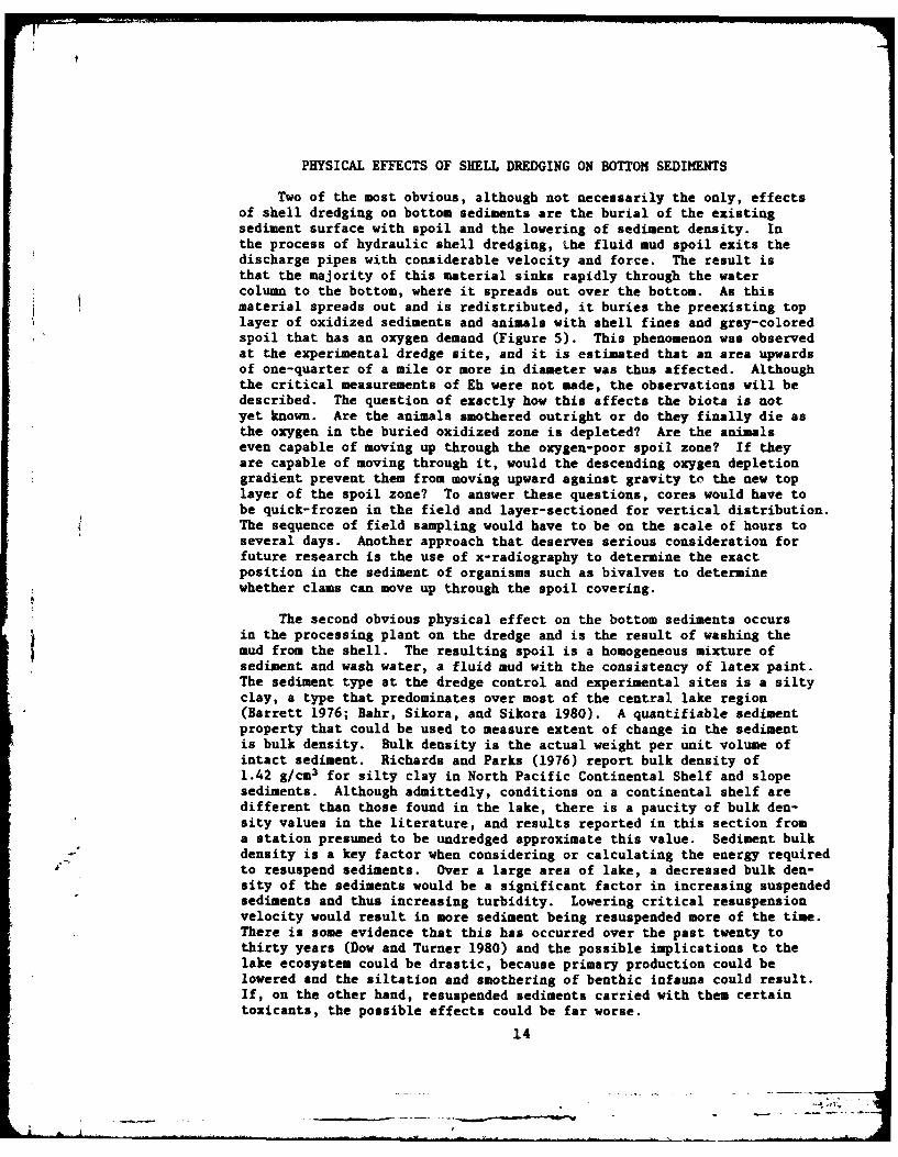
Two of the most obvious, although not necessarily the only, effectsof shell dredging on bottom sediments are the burial of the existingsediment surface with spoil and the lowering of sediment density. Inthe process of hydraulic shell dredging, Lhe fluid mud spoil exits thedischarge pipes with considerable velocity and force. The result isthat the majority of this material sinks rapidly through the watercolumn to the bottom, where it spreads out over the bottom. As thismaterial spreads out and is redistributed, it buries the preexisting toplayer of oxidized sediments and animals with shell fines and gray-coloredspoil that has an oxygen demand (Figure 5). This phenomenon was observedat the experimental dredge site, and it is estimated that an area upwardsof one-quarter of a mile or more in diameter was thus affected. Althoughthe critical measurements of Eh were not made, the observations will bedescribed. The question of exactly how this affects the biota is notyet known. Are the animals smothered outright or do they finally die asthe oxygen in the buried oxidized zone is depleted? Are the animalseven capable of moving up through the oxygen-poor spoil zone? If theyare capable of moving through it, would the descending oxygen depletiongradient prevent them from moving upward against gravity to the new toplayer of the spoil zone? To answer these questions, cores would have tobe quick-frozen in the field and layer-sectioned for vertical distribution.The seqlence of field sampling would have to be on the scale of hours toseveral days. Another approach that deserves serious consideration forfuture research is the use of x-radiography to determine the exactposition in the sediment of organisms such as bivalves to determinewhether clams can move up through the spoil covering.
The second obvious physical effect on the bottom sediments occursin the processing plant on the dredge and is the result of washing themud from the shell. The resulting spoil is a homogeneous mixture ofsediment and wash water, a fluid mud with the consistency of latex paint.The sediment type at the dredge control and experimental sites is a siltyclay, a type that predominates over most of the central lake region(Barrett 1976; Bahr, Sikora, and Sikora 1980). A quantifiable sedimentproperty that could be used to measure extent of change in the sedimentis bulk density. Bulk density is the actual weight per unit volume ofintact sediment. Richards and Parks (1976) report bulk density of1.42 g/cm 3 for silty clay in North Pacific Continental Shelf and slopesediments. Although admittedly, conditions on a continental shelf aredifferent than those found in the lake, there is a paucity of bulk den-sity values in the literature, and results reported in this section froma station presumed to be undredged approximate this value. Sediment bulkdensity is a key factor when considering or calculating the energy requiredto resuspend sediments. Over a large area of lake, a decreased bulk den-sity of the sediments would be a significant factor in increasing suspendedsediments and thus increasing turbidity. Lowering critical resuspensionvelocity would result in more sediment being resuspended more of the time.There is some evidence that this has occurred over the past twenty tothirty years (Dow and Turner 1980) and the possible implications to thelake ecosystem could be drastic, because primary production could belowered and the siltation and smothering of benthic infauna could result.If, on the other hand, resuspended sediments carried with them certaintoxicants, the possible effects could be far worse.
14
* - - -

44 -P -A,
a 041 ONZ Iw
V 0 ~#so 0 u -~
W0 OOs *rA
41+. K 4.
Z#44
0.0 :% ' O .0
%0. 4 if
Lai 00 V
0 0
J a 00 S.' 5' #4 Vr4
#V - Ii. NS. 00 0
u
$, 4 0
A Az
M3N HIMILVKIXOvddV
15
Methods
Bulk density is the actual weight per unit volume of intact sediment,with differences between sediments of same grain size and similar organiccontent being the result of sediment consolidation. Consolidation ofsediments, corresponding most closely to compaction in geological termi-nology, is defined as "every process involving a decrease of the watercontent of a saturated sediment without replacement of the water by air"(Terzaghi 1943) or "the gradual process which involves, simultaneously,a slow escape of water and a gradual compression, and which also involvesa gradual pressure adjustment" (Taylor 1948). Bulk density can be usedas a measure of the consolidation state provided that the grain sizedistribution is taken into account. In the present study, all thesediment is of the silty clay type, thus making comparisons possible.We measured both in situ bulk densities at a number of stations main-tained in the concurrent benthic characterization study and bulk densityover time in a laboratory consolidation experiment on dredge spoilobtained from the dredge Lacombe while operating in the western part ofthe lake south of station 7 and west of station 8 on June 28, 1980, (thedredge Lacombe was previously the Kathy L., as described by GSRI 1974).Fifty polyethylene buckets with tight-sealing lids of 18 liter capacitywere filled with spoil by means of a 5 cm hose fitted to the lower sideof the discharge pipe of the dredge. The spoil was brought back to thelaboratory and dumped into 16 columns made from 3.2 mm thick, 30 cmdiameter PVC pipe with 6.4 am PVC bottoms. The columns were placed intwo racks holding eight columns each and were filled to a height of75 cm. These columns were fitted with the same tight-sealing lids bycutting off the top portion of the buckets and riveting them to the topsof the columns and sealing them with silicone caulking. The lids, afterbeing placed on the columns, were taped with electrical tape to producea completely watertight seal. The columns were sampled for bulk densityon days 0, 6, 12, 18, 27, and 226.
Bulk density samples were obtained using core tubes, which w(.rtmade of 5 cm long core segnents taped together with waterproof tp'P Loform one core tube. The in situ samples were taken with core tubesconstructed of core segments cut from standard 50 cc plastic syringes,2.55 cm in diameter, with the leading segment beveled to form a cuttingedge. Each core segment was numbered and premeasured fer volume. Thecore tube was inserted slowly into the box core sample with a gentlerotation. After removing the core tube containing the sample, theoutside was washed and the tape holding each segment was cut, and apiece of preweighed aluminum foil was inserted as the segment was re-moved and placed in a preweighed plastic vial with a tight-fitting cap.The samples were refrigerated, brought back to the laboratory, andweighed. Total sediment weights for each 5 cm sediment interval werecalculated by subtracting plastic vial weight, core segment weight, andaluminum foil weight for each sample. Sediment bulk densities in g/cm
3
were calculated by dividing total sediment weight by the core segmentvolume. Bulk densities for the consolidation experiment were taken in asimilar manner; glass core tube segments 5 cm long and 3.3 cm in diameter,however, were used. Also, because of the nature of the spoil, it wasnot possible to insert a core tube by gently rotating it. A smallvibro-engraver was attached to the top of the core by rubber bands,
16

making a minivibracorer. This device allowed the core tube to be in-serted with minimal effects on the sediment. No aluminum foil was used;rather, the tape was cut with a modified spatula, sharpened on theleading edge and with a hole cut toward the back over a screw cap. Thisallowed the sample and core segment to be slid back and dropped directlyin the plastic jar with a tight lid. Bulk densities were determined inthe same manner as the in situ samples.
Results
The initial bulk density of the spoil was 1.22 g/cm3 and was uniformthroughout the column. By day 6, the sediment surface had dropped 6 cm.The bulk densities by 5 cm depth intervals, however, were not uniformthroughout the column but increased with depth to 1.26 g/cm3 5 cm abovethe bottom (Figure 6). The botto-most 5 cm was not sampled for bulkdensity to ensure against even the slighest disruption of this segmentduring capping and removal of core tube from the column. The topmost5 cm segment remained at the initial bulk density of 1.22 g/cm 3. As theexperiment progressed, the sediment surface continued to drop, 8.7 cm byday 12, 11.5 by day 18, and 13.5 by day 27. The topmost 5 cm segmentgained very little in bulk density, rising to 1.23 on days 12 and 18 andto 1.24 on day 27. The lower segments in the column continued to gainin bulk density from 1.29 g/cm3 to 1.35 g/cm 3 on day 27. The spoilsediment begins consolidating at the bottom of the column, displacingwater upwards through the upper segments of sediment. This movement ofwater apparently keeps the upper segments at a lower bulk density notsignificantly different from the initial density. By day 226, thebottom bulk densities are approaching reported literature values of1.42 g/cm2 for undredged silty clay, and the upper segments have gainedconsiderably in density. The sediment surface has dropped 29.3 cm, or39% of the height of the sediment column, although the rate of drop hasdeclined to less than an average of 0.7 ,--/day (Figure 7).
The in situ bulk densities are compared for the dredging controlstation, the dredging experimental station, and stations 2, 8, and 12from the benthic characterization study as well as day 12 and 226 of theconsolidation experiment (Table 4). These stations are all of the siltyclay sediment type with similar organic contents (Table 5).
Discussion
The results of the sediment consolidation experiment were quite un-expected, particularly the non-uniform consolidation with lower segmentsconsolidating at a faster rate. The displaced water, however, causedthe upper layers of sediment to remain unconsolidated, and it is in theupper layers, particularly the top 5 cm, where the benthic fauna reside.The entire consolidation process appears to take place rather rapidly,and we believe it is not so rapid in the field. If one looks at thedrop in the sediment surface, one might conclude that a trench dug by adredge and filled with spoil which issued from the back end got deeperas time progressed. This is probably not the case; dredge cuts wouldtend to fill in over time. The movement of sediment by wave action and
17

4-4 I
aav
F40
~ K0. 1C,4
~ v 04 04
N ~ ~ ~ ~ ~ ~ . 00 N Ac - 0 0 0 0 Ipf
-~~~ -0 -w -*~ U4at
0
0 0
0S41
a0 K~
-- - -- -

0 a
93
.0
r4
0tU
.4
0
:C
194

Table 4. Sediment bulk densities, by depth, at Dredging Control Station (DC)
and Dredging Experimental Station (DX), Day 12 and Day 226 of theconsolidation experiment and three stations from the benthiccharacterization study of the same silty-clay sediment type
Depth 1 2 3 4 5 6 7 8cm STA 2 DX DC DAY 12 DAY 226 DAY 226 STA 12 STA 8
0
1.28 1.31 1.29 1.23 1.31 1.28 1.17
51.41 1.15 1.22 1.24 1.34 1.27 1.36
10
1.41 1.23 1.26 1.24 1.37 1.25 1.31
15
1.43 1.28 1.23 1.25 1.38 1.27 1.30
20
1.43 1.42 1.26 1.24 1.40 1.31 1.30 1.30
25
1.45 1.34 1.24 1.25 1.41 1.34 1.31 1.32
30
1.29 1.27 1.25 1.42 1.37 1.33 1.36
35
1.24 1.42 1.38 1.35
40
1.27 1.40
45
1.25 1.41
50
1.27 1.42
55
1.29 1.42
60
20

Table 5. Total organic carbon analysis in percent weight, by depth, atthree stations from the benthic characterization study,Dredging Control Station (DC), Dredging Experimental Station (DX)
Depth STA 2 STA 8 STA 12 DC DXcm
0
1.52 2.05 1.44 1.83 1.75
5
1.77 0.96 1.27 1.70 1.66
10
1.21 1.54 1.21 1.85 1.80
15
1.23 1.41 1.11 1.86 1.71
20
1.10 1.67 1.26 1.33 1.67
25
1.15 0,89 1.31 1.68 1.65
30
35 0.79 1.41 1.17 1.73
1.79
40
21

its sedimentation in a trench, however, would provide a continual, lowbulk density environment for benthic organisms. Large, dense benthicorganisms such as large Rangia may not be able to survive in these lowdensity sediments, which might be a contributing factor in explainingthe paucity of large living Rangia presently in the lake, as found bythis study and the concurrent benthic characterization study.
During a 1954 quantitative survey of the benthos Darnell (unpub-lished manuscript) recorded densities of 141 Rangia per m2 larger than20 m at a station closest to the experimental dredging and controlstations of the present study. During the present study, at the dredgingcontrol station, we found from 36 box core samples a mean of 0.9 ± 0.9per m2 of Rangia larger than 20 m. In the eastern part of the lake atsix stations, all of which were out from the periphery, Darnell in his1954 survey found densities of Rangia larger than 20 m to be 173 ±31.1/M2 from 12 Peterson grab samples. Tarver (1973) reported thatduring his study of Rangia cuneata, virtually no clams larger than 16 -were found in areas which were continually dredged, and that easternLake Pontchartrain was void of this size clam although the periphery ofthe lake had large concentrations.
It seems certain that conditions in the open lake that are detri-mental to large Rangia have arisen in the past 26 years. Both lowdensity sediments unable to physically support large Rangia as well asincreased suspended sediments in the near bottom environment couldcontribute to these detrimental conditions. We know that dredgingresults in the production of low density sediments. Future research isneeded to investigate the suspended sediments in the near-bottom envi-ronment.
The precise bulk density value of the sediments at the sediment-waterinterface is unknown and difficult to measure. A further complicatingfactor is the existence of a fluffy, organic-rich layer at this interface.The bulk density values reported in Table 4 for the uppermost segment ofeach column are for the first 5 cm of depth as a unit. This segmentdoes not appear very different from the in situ stations except, perhaps,station 8 with a value of 1.17. However, attention should be focused onthe 5-10 cm depth that supports the upper 5 cm. The dredging experi-mental station, dredging control staton, and station 12 all exhibitlower densities at the 5-10 cm depth. Conceivably, a large Rangia, of40-50 mm, lying under the sediment surface would just about protrudeinto the 5-10 cm segment with its shell, while its foot would penetratewell below 5 cm. Also, the activity of the animal would t' nd to disruptthe sediment immediately surrounding it. If a clam were to experience
- continual sinking, with a continuous expenditure of energy required tokeep its siphons above the surface of the sediments, (a situation forwhich it is not adapted), its growth would be inhibited and its survivalwould be threatened. If additional environmental stresses were added,survival could become impossible.
A comparison of the bulk densities by depth in Table 4 yields somestriking similarities and a notable exception. This exception is sta-tion 2, with bulk densities approaching and exceeding the literaturevalue of 1.42 for silty clay (Richards and Parks 1976). These data
22
________ - --'-~------- ~ . -..-.- .--
,-77-.
indicate that station 2 has not been dredged. Conversely, comparing thedredging control station to day 12 of the consolidation experiment, theyappear quite similar, as do the top four segments at station 12. If wereference the sediment column of day 226 to the bottom, as in column 6,we find striking similarities at the same depths at station 12 andstation 8. Station 12 seems to behave as the postulated model for adredge cut in the field, with the original spoil surface sinking to adepth of 20 cm and additional low density material filling in on top. Asimilar sequence may have taken place at station 8 over a longer periodof time. The dredging experimental station showed alternately very lowdensities and higher densities, which might be the result of slumping.Station 12 appears to have been heavily dredged; nine box cores takenquarterly yielded a mean of 32 g of shell retained on one-half inch meshscreen (compared to means of 1620 g at station DX and 750 g at station DC).In a 1954 survey of the benthos, Darnell (unpublished manuscript) had astation in almost exactly the same location, and he recorded a mean of132/M2 of Rangia larger than 20 m. Shells from these animals alonewould amount to more than 32 g per box core. If we accept station 12 ashaving been dredged, then we must also accept the dredging controlstation as having been dredged at some time prior to construction of theCauseway.
In perspective then, the results found in this study obtain primarilyfrom differences between a dredged station and a station that has notbeen dredged in at least 27 years. We do not have a pristine, undredgedstation to compare with, nor do we have data from a pristine Lake Pontchar-train before dredging. Consequently we are comparing the effects ofdredging on a benthic community that has survived dredging for 48 yearsand may indeed be composed of only the hardiest organisms of the originalcommunity.
23

THE EFFECTS OF SHELL DREDGING ON THE NUTRIENT ANDHEAVY METAL CHEMISTRY OF THE WATERS AND
SEDIMENTS OF LAKE PONTCHARTRAIN
Introduction
A control and a test or experimental dredging site were establishedwithin a central area of the lake which had not been disturbed recentlyby hydraulic shell dredging. Filtered and unfiltered samples were col-lected prior to dredging from a depth of one meter (subsequently referredto as mid-water) and from the water/sediment interface; sediment sampleswere also taken. The concentrations of nitrogen and phosphorus compoundsand of the heavy metals lead, zinc, copper, iron, manganese, and cadmiumwere determined. The same measurements were made on mid-water samplescollected from the test site at the point of dredging, and one hour aftercompletion of dredging on the same day. A full quota of samples wastaken at the dredged site on Days 1 and 2 following dredging, and fromDay 5 onwards, water and sediments were sampled at both control anddredged sites (see Table 6).
Literature Review
Nutrients
Mortimer (1941) he found that phosphorus was released from anaerobicsediment systems when the ferric iron content was reduced to ferrousiron. He proposed that the capacity of the sediments to hold phosphoruswas related directly to the presence of ferric iron. The reduction ofthe mud surface corresponded with an increase in the transport of nutri-ents to the overlying water (Mortimer 1941 and 1942).
It has since been shown that phosphorus is released from sedimentsunder aerobic conditions (Olsen 1964). The uptake of phosphorus in thewater by algae was followed by the release of phosphorus from the sedi-ments, and in oxidized sediments the exchange was more complete. Gahlerperformed laboratory experiments which showed that the concentrations ofnitrogen and phosphorus increased in overlying water in both aerobic andanaerobic environments (Gahler 1969). This increase in nitrogen and phos-phorus concentrations was associated with resuspension of the sediments.
has The ability of sediments to supply nutrients to the water columnhas been much studied. Sediments and interstitial waters have beenanalyzed chemically. Livingstone and Boykin (1962) extracted the sedi-ment cores from a Connecticut pond with deionized water. They foundthat more phosphorus was released from shallow cores (10 cm) than fromdeeper cores (10 m). It was observed that as the ratio of water tosediment increased, the amount of phosphorus released in solution alsoincreased. The time basis of the phosphorus release was not reported.
Byrnes et al. (1972) measured the exchange of (NH4 )-N across asediment/water interface. Sediments at rest were spiked with additional
24

414
fA U3U~v
0*
-- C" VCp%01P 4 1
040
oo ~ ~ ~ 0 00.. 00C 4&MI - " l l
441
;o
~0
C4 C ( N N0
a c
A~ co V2 02V4
64 I
25~El

nitrogen and+the (NH4)-N rate of release determined. The sedimentsreleased (NH4)-N at a linear rate for a period of 8 hours.
Considering the results of Gahler's experiments in which it wasshown that the nutrients, artificially released into the water column,supported algal growth, there seems little doubt that sediments containnitrogen and phosphorus in forms releasable to overlying water undereither aerobic or anaerobic conditions. Also, the released phosphorusand nitrogen compounds are available as growth supporting nutrients.
Once it was thought that only thin layers of surface mud wereinvolved in water/sediment exchange processes. However, Bricker andTroup (1975) studied the behavior of the sediment/interstitial waterenvironment and the importance of this environment to the chemistry ofthe estuarine system in Chesapeake Bay. It was reported that a rapidexchange of nutrients between overlying water and the upper part of thesediment column took place to depths of 30 cm. Nutrients in solutionwere exchanged across the water/sediment interface in response to thephysical disturbance of the sediments by tidal or storm-induced currents.Hynes and Greib (1970) found that inorganic phosphate and (NH4)-N movedeasily through anaerobic sediments by diffusion mechanisms, suggestingthat more than a thin surface layer was involved in exchange processeswith the overlying water. Porcella et al. (1970) experimented withwater columns over sediment cores 15 cm long. Phosphorus was releasedinto the water from the entire length of the core.
The behavior of phosphorus in Wisconsin lakes has been reported byBortleson (1970) and Sridharan (1973). Lee (1970) concluded from anexamination of these reports that there was evidence for the existenceof a sediment mixing zone which extends to at least 10 cm below thewater/sediment interface. It was suggested that the composition of thesediment and the mixing energy of the system, be it natural or artificial,governed the depth to which sediments were involved in exchange processeswith overlying water.
The results of many studies of the effects of disturbance or agita-tion on the release of nutrients from sediments have been reported.There is general agreement that agitation of sediments causes theirresuspension into the water column and promotes the release of nutrients.
Zicker et al. (1956) buried labelled phosphorus at various depthsin sediment cores and measured the release of phosphorus to the water onagitation of the sediments. An increase in the release of phosphorus tothe water was measured and was thought to be due to an increase in thesurface area of sediment exposed to the water column. Austin and Lee(1973) found that active mixing of sediments caused the release o0fnitrogen to be fifty times greater than that released from undisturbedsediments.
Ruttner writes in Fundamentals of Limnology (1963) that the mixingof natural water sediments is associated with the transport of chemicalmaterials from the sediment to the water column. Wind-induced currents,eddies, and benthic activity are cited as mixing mechanisms which induceexchange between sediments and water. Gahler (1969) observed large
26

increases in total phosphorus and (NH4)-N concentrations of an area ofLake Klamath where sediments had been mixed by benthic algae.
Austin and Lee (1973) found that where there was little mixing ofthe sediment/water interface. Nutrients were held in the sediments andwere not released in any quantity to the water. It was expected thatthe very drastic mixing of sediments occurring during shell dredgingwould cause large increases of nutrients to the water column.
Summary
There is much available information on the nutrient composition andbehavior of water/sediment systems.
Phosphorus and nitrogen compounds are released from sediments tooverlying water in forms suitable for uptake as nutrients.
Nutrients are released under aerobic and anaerobic conditions, withassociated resuspension of sediments, and inorganic phosphate and (NH4 )-Ndiffuse easily through the sediments.
The transport of nutrients to the water column takes place fromdepths of up to 30 cm within the sediment.
Sediments at rest release added nutrients into the overlying waterat a linear rate for a period of eight hours.
The natural or experimental agitation of sediments causes therelease of nitrogen in quantities up to fifty times greater than thosereleased from undisturbed sediments.
Any mixing mechanisms, no matter how minimal, induce large increasesin the release of nutrients from more than the surface layer of thesediment.
It is therefore expected that a study of the effects of shelldredging on the water and sediment chemistry of Lake Pontchartrain willshow increases in the nitrogen and phosphorus content of the water attimes close to the dredging operation. These increases in the water mayalso be associated with decreases in the concentrations of nitrogen andphosphorus in the dredged sediments.
Metals
Heavy metals are known to be toxic at certain concentrations toaquatic organisms. The Environmental Protection Agency (EPA) has pre-pared Quality Criteria for Water (1976) giving acceptable levels ofheavy metals (Table 7).
27

Table 7. Criteria for water quality-heavy metal concentrations (EPA 1976)
Fresh Water Marine WaterElement Pg/l pg/l
Cd <30 10Cu >30 50Fe 300 300Mn 50 100Pb 30 50Zn 1 100
These criteria were developed from bioassay studies in which orga-nisms were exposed to metals in solution. Criteria which govern thebehavior of metals in solution cannot be applied directly to particulatematerial or to sediments. The metal composition of the sediment may notbe related directly to its pollutional characteristics when resuspendedin water, as happens during dredging operations (Windom 1973).
Windom prepared criteria for a few metals in sediments suitable foroverboard disposal in marine waters which were used by the U.S. EPARegion IX (Table 8).
Table 8. U.S. EPA Region IX metal criteria for the suitability ofsediments for overboard disposal
Element Criteria mg/Kg dry weight
Cd 2Cu 50Pb 50Zn 75
The presence or absence of oxygen is considered to have greatinfluence on the release of metals from dredged materials (Lee 1975).Mortimer (1971) observed that a progressive decline in oxygen concentra-tion to analytical zero at the sediment interface of Esthwaite waterscould be correlated with the mobilization of iron and manganese in thesediments and also with their transfer into the water. Phosphate andammonia were released concurrently.
Mortimer further suggested that an oxidized microlayer that existedat the sediment interface trapped iron and manganese effectively.
Gorham and Swaine (1965) found an increase in the concentrations ofiron and manganese in oxidized sediments. They were of the opinion that
28

the ferro manganese minerals were capable of scavenging other metalssuch as lead and zinc from the water and accumulating them in the sedi-ments. In 1968 Jenne wrote that hydrous iron and manganese oxidesplayed a significant role in the control of the levels of manganese,iron, copper, and zinc in soils and water.
The changes in heavy metal concentrations resulting from maintenancedredging were explained by Windom (1973) in terms of the reaction ofhydrous iron oxide to the concentration of dissolved oxygen. In separatestudies, May (1973) and Lee (1975) concluded that oxygen in solution cancontrol the release of metals from dredged material. May (1973) monitoredthe concentrations of various metals in filtered water samples before,during, and after dredging operations and detected no significant change.
Windom (1973) studied the effects of dredging on the water qualityof several estuaries of the southeastern United States. Sediment sampleswere dispersed in overlying water, maintaining the sediment-to-waterproportions of dredge effluent. The concentrations of iron and othermetals increased initially in the water, followed by some decrease.Eventually, after several days, an increase to the original concentra-tion levels, or higher, was observed.
These changes in the metal content of the water were explained interms of the behavior of iron in natural waters. Reduced ferrous iron,released from dredged material, is oxidized to insoluble ferric iron inthe water column and precipitated with the settling of the sediments.Other metals that are adsorbed on the insoluble ferric iron precipitateare carried down and deposited on the bottom. With a return to reducedconditions, the metals are released, and shortly thereafter the originalmetal concentrations are reestablished.
The release of iron from the sediments of Mobile Bay was studiedduring dredging. During the first day of dredging, an increase wasobserved, followed by a rapid decline of a further two days, and areturn to the original level after two weeks (May 1973).
Lee (1975) developed an elutriate test in the laboratory, in whichthe environmental conditions under which metals were released duringdisposal of dredged sediments were simulated. The results of thisexperimental work indicated that under oxidizing conditions manganesewas released from both freshwater and marine sediments and zinc wasremoved from solution. The release of manganese and the removal of zincwere proportional to the percentage of sediment in the total volume, upto 20% sediment.
In anaerobic conditions, iron, manganese, and lead were releasedinto solution. Greater quantities of manganese were released anaerobi-cally than were released aerobically. Variations in the oxidizingconditions did not affect significantly the concentrations of copper andcadmium.
29
- -.t

Sumaary
The indications from the literature are that the response of theheavy metal content of water and sediments to dredging is controlledlargely by the reactions of hydrous iron and manganese oxides. Iron inparticular is more soluble in the reduced form.
When anaerobic sediments containing reduced iron oxide come intocontact with air and the aerated water column during dredging, metalconcentrations in the water increase initially. The reduced iron isoxidized to ferric oxide in the aerobic conditions. The insolubleferric iron precipitates out and is deposited on the lake bottom withthe resettling of the suspended sediments that follow disposal ofdredged material. Other metals adsorbed on the ferric oxide precipitateare scavenged from the water column to accumulate in the bottom sediments.
Dredging activity would, therefore, very temporarily be expected toincrease metal concentrations in the water column. Soon, however, underoxidizing conditions, decreases in metal concentrations should follow asthey are removed by adsorption on precipitating ferric oxide. With thereestablishment of reducing conditions within the redeposited dredgedmaterial, some resolution of metals should occur, and within days,initial concentrations be restored in the water column.
Materials and Methods
Sample Collection and Preservation
Water samples were collected in 1000 ml polyethylene bottles thathad been acid-washed previously in the laboratory. Raw water, filteredin the field through a 0.45p membrane Millepore filter, constitutedfiltered water. All water samples, whether filtered or unfiltered, .wereplaced on dry ice in the field and transported to the laboratory freezer,where they were stored until time of analysis.
The sediment samples were taken with a box corer. Aliquots ofsediment were placed in plastic Ziploc bags, frozen on dry ice, andtransferred to the laboratory freezer to await analysis. Interfacesamples were siphoned from the sediment-water interface into polyeth-ylene bottles and were treated as above.
Nutrients
Pretreatment of Samples
Immediately prior to analysis, samples of filtered water and unfil-tered mid-water were allowed to defrost undeT cold running water. Thefiltered water samples were analyzed for (NH4)-N, total inorganic nitrogen(T.I.N.) and orthophosphate (ortho P04). The concentration of totalphosphorus (tot-P) was measured in unfiltered mid-water samples.
30
Due to highly varying amounts of sediment in unfiltered interfacewater samples, it was decided to express the concentrations of totalphosphorus (tot-P) and total Kjeldahl nitrogen (tot Kj-N) on a percentagedry weight of sediment basis rather than per unit volume of water. Forthis reason, unfiltered interface water was defrosted and filteredthrough a 0.45p Millepore membrane filter. The particulate material wasoven-dried at 60*C for 24 hours, finely ground, and stored. The dryparticulate was analyzed for tot-P and tot Kj-N.
Frozen sediment samples were shattered while still in the Ziplocbags. Randomly selected pieces were oven-dried at 600C for 24 hours,finely ground, and stored. As with the particulate from the interfacewater, the concentrations of tot-P and tot Kj-N were measured.
Analytical Methods
A. Filtered Water
1. (N)-N. Filtered water that had been defrosted was shakenthoroughly, and a 25 ml aliquot was pipetted into a 100 mldistillation flask. The aliquot was male basic by the addi-tion of 0.05 g light MgO, converting NH4 ions into NH3moleculgs. The basic sample was steam distilled for 3 minuteson a generator regulated to produce distillate at a rate of6.5 ml/min. The distillate was collected in a 50 ml volume-tric flask containing 1 ml 0.1 N.HC, thus stabilizing theNH3 . The NH3 was oxidized to NO2 with a sodium hypochlorite/potassium bromide/NaOH solution, and the oxidation allowed toproceed for 30 minutes. Any excess oxidizing agent was poi-soned by the addition of a sodium arsenite solution. After 5minutes, the NO2 was complexed with sulphanilamide in acidsolution. Finally, diazotization by napthyl ethylene diaminedihydrochloride resulted in the formation of a highly coloredazo dye, the absorbance of which was measured spectrophotome-trically at 543 nm (Strickland and Parsons 1972, Ho andSchneider 1974).
2. T.I.N. (NH4 + NO; + NO;)-N. A 25 ml volume of filtered waterwas measured into a 100 mI distillation flask. Light MgO wasagain added to convert NH4to NH3 . To reduce NO3 and NO2 toNH3, 0.3 g Devardo's alloy was added. With all nitrogen inthe form of NH3, the treated sample was steam distilled for 4
- minutes, and the distillate was collected in a 50 ml volume-tric flask containing 1 ml 0.1 N HCl. The subsequent treat-men and color development followed that given above for(NH4)-N (Ho and Barrett 1975).
3. Orthophosphate - (Inorganic, molybdate reactive phosphorus).A 100 ml sample of filtered water was pipetted into a 250 mlseparatory funnel, which had been acid-washed, and stored fullof 0.4 N HC until needed. Five ml of 25% H2SO4 were added,followed immediately by 5 ml ammonium molybdate solution, to
31
Li : :.

I/
form a phosphomolybdate complex. Reaction time was 5 minutes.The phosphomolybdate complex was extracted into ethyl acetate,and the bottom aqueous layer was discarded. Ascorbic acidsolution and potassium antimonyl tartrate solution were addedin quick succession, the mixture was shaken, and on separation,the aqueous layer was again discarded. The resulting blueorganic layer containing the reduced phosphomolybdate complexwas drained off and made up to 10 ml with 90% ethyl alcohol.Absorbance was measured spectrophotometrically at 690 nagainst a cell blank of 50% alcohol. The above method was amodification of Strickland and Parsons (1972) by Ho andSchneider (1974).
B. Unfiltered Mid-water
4. Total Phosphorus (tot. inorg P + tot. ors P). A 50 ml aliquotof unfiltered mid-water was measured into a 125 ml Erlenmeyerflask, and 1 ml 75% HIS04 added. Then, 0.2 g potassium persul-phate was added, and the whole was digested for 1 hr at 90°C(Standard Methods, Am. Public Health Assoc. 1976). During theoxidation with persulphate, oxidizable organic phosphorus,whether in soluble or particulate form, was released as inor-ganic phosphorus. With the total phosphorus in the inorganicmolybdate reactive form, the digest was diluted and transferredto a separatory funnel, and the phosphorus content was measuredas for orthophosphate.
C. Interface Particulate and Sediments
5. Total Kjeldahl Nitrogen. The Kjeldahl method, essentially awet oxidation procedure, was used+(Bremner 1965). The nitrogenof the sample was converted to NH4 by digestion with concen-trated HA04 , containing Kjeldahl catalyst, which promoted theconversion. The NH,4 became NH3 on distillation of the digestwith strong alkali, and the NH3 content of the sample wasdetermined. Fifty mg dry sediment were placed in a digestiontube, to which 1 g Kjeldahl catalyst and 3 ml concemtratedH2SO4 were added. The sample was digested for 1.5 hours at1500C, followed by 3.75 hours at 3750C. On cooling, thedigest was diluted to 25 ml with distilled water, and trans-ferred to a 100 ml distillation flask. Thirteen ml 10 N NaOHwere added, and the sample steam was distilled for 3.5 minutes.The distillate was collected in a 50 ml volumetric flaskcontaining 1 ml 0.1 N HCI. A color development was affectedusing Nessler's reagent, and the sample absorbance was deter-mined spectrophotometrically at 402 nm against a referencecell of distilled water (Handbook of Chemistry and Physics1977).
6. Total Phosphorus (tot. inorg. P + tot. or&. P). One hundredmg of dry sample were digested following the Kjeldahl wetoxidation procedure. This was a modification by Kemp of the
32

Bremner method (Kemp personal communication, Bremner i965).As was the case with the persulphate digestion of unfilteredmid-water, organic phosphorus was released in the inorganicmolybdate reactive form and therefore was measurable as fororthophosphate.
Metal Analysis
Pretreatment of Samples
Before analysis, filtered water and unfiltered mid-water sampleswere defrosted at room temperature. Two ml redistilled conc. HN03 wereadded to each liter of water sample, producing a pH value 12. Thusacidified, the water samples were left to stand for a period not lessthan 48 hr prior to analysis for metal content.
Similar to the nutrient analyses, the problem of the highly varyingamounts of sediment in unfiltered interface water samples prompted thefilteration of interface water through a 0.45m Millepore membrane filter.The particulate material was subsequently treated as sediment, withmetal content expressed on a dry weight basis.
Frozen sediment samples were broken into small pieces, and repre-sentative portions were oven-dried at 60°C, finely ground, and storeduntil analysis.
Analytical Methods
A. Sediment and Interface Particulate
A 2.5 g quantity of dry, ground sample was placed in a 125 mlErlenmeyer flask containing 25 ml distilled water and 25 ml redistilledconcentrated HN03. The digestion mixture was heated at 500C for 6 hr ina hot water bath, with frequent shaking.
After digestion, the sample was cooled and filtered through a 0.45pMillepore filter. The filtrate plus washings of the digest flask weretransferred to a 100 ml volumetric flask and made up to volume. Areagent blank of 25 ml distilled water/25 ml conc. HN0 3 was carried
- throughout the digestion and final dilution (Villa, and Johnson 1974).
The concentrations of lead, zinc, and copper in the digests weremeasured by flame atomic absorption techniques using a Perkin Elmer 360Atomic Absorption Spectrophotometer. The preparation of standard solutionsand the procedure for the measurement of individual metal concentrationsin the digests was followed from Analytical Methods for Atomic AbsorptionSpectrophotometry, Perkin Elmer (19i6).
To keep the concentrations of iron and manganese within the linearrange of absorbance, the digests required a further 1:25 dilution beforemeasurement by flame techniques.
33
.............
The concentrations of cadmium in the digests were low and werebeyond the lower limits of detection by flame methods. Cadmium in thedigests was measured by flameless atomic absorption using the method ofstandard additions.
Ten ml volumes of digest were spiked with 50-200 p1 volumes of a1 mg/l Cd standard solution, resulting in added concentrations of metalin the 5-20 pg/l range. To reduce matrix effects due to salinity, anequal volume of 5% NH4NO3 solution was injected into the graphite tubebefore injection of a 20 or 50 p1 volume of straight digest or digestspiked to a known concentration with additional cadmium. Drying, char-ring, and atomizing times and temperatures were as recommended by PerkinElmer for the HGA 2100 Graphite Furnace (Perkin Elmer 1976). Absorbancereadings were recorded for each concentration of added cadmium, i.e., 0,5, 10, 15 pg/l, etc. Absorbance readings were plotted against the addedconcentrations of metal. An extrapolation of the resulting straightline produced an intercept on the concentration axis equal to the concen-tration of metal in the digest solution.
B. Filtered Water and Unfiltered Mid-water
When the method of standard additions was applied to unfilteredmid-water samples, it was found that even after several additions ofmetal, particularly lead, there was no increase in absorbance readings.This effect was presumed to be due to absorbance of metal on the smallamounts of particulate material present in the unfiltered water since nosimilar effect was found with filtered water samples. Further acidifi-cation to pH 1 with conc. HN03 prevented the absorbance of added metalon particulate material and kept added metal in solution.
At the same time, the method of Sholkovitz was used (Sholkovitz1978). This method gave values of metal concentrations that were equiva-lent to and as reproducible as those obtained from graphite heatedatomization, applying standard additions. Sholkovitz iethod also hadthe advantage of being less laborious and less time-consuming.
One hundred ml volumes of filtered water and unfiltered mid-watersamples, acidified to pH 1 for a minimum of 2 days, were evaporated untilalmost dry. The final volume was adjusted to 5 or 10 ml with 4 N HNO3.This ten-or twentyfold increase allowed the concentrations of lead, copper,zinc, iron, and manganese to be determined by flame atomic absorption methods.
As was done with the sediment digest preparations, cadmium in theheat concentrated samples was measured by flameless atomic absorption,applying the method of standard additions.
Results
Precision of Estimates
Data variability arose from two sources: from that inherent in the
laboratory methods, and from that due to field sampling techniques. The
34
laboratory precision of each analytical method was computed from sets of3 or 5 aliquots taken from one field sample. The field sampling variationwas estimated from sets of 3 or 5 field samples.
The variations in laboratory method and in field sampling wereexpressed as mean coefficients of variation. For each set, the ratio ofthe standard deviation to the mean value of a measurement was calculatedas a percentage. The average of the percentages was taken as an estima-tion of variation. The variation values are presented where relevant aspart of the tables of results.
Nutrients
Mid-Water Analyses
The results of the nutrient analyses for filtered and unfilteredmid-water samples are given in Tables 9 and 10, together with Figures 8-11.
The concentration of (N14)-N ranged from 2.4 - 103 pg/l at thedredged site, and from 0 - 33 pg/l at the control site. The concentra-tion of total inorganic nitrogen was in the range 16 - 422 pg/l at thedredged site, and 10 - 380 pg/l at the control site. Orthophosphatevalues were very comparable at both sites, being in the range 12 - 44pg/l. Levels of total phosphorus were also in the same range at bothsites, namely 38 - 66 pg/l.
Before dredging began, equal concentrations of nitrogen (22 pg/l)in the form of (NH4)-N were found at the control and dredging sites.With the onset of dredging, the concentration rose immediately to 49pg/l at the dredging site. Within 2-5 days the level had dropped sub-stantially to 16 pg/l (Figure 8).
As time progressed, however, increased concentrations of (NH4)-N inmid-water samples from the dredging site were not matched with increasesat the control site. Application of the "student's" test to the datafor 20. 50 and 259 days following dredging showed that the concentrationof (NH4)-N was significantly higher at the dredging site. Significancewas at the 0.5 confidence level.
Total Inorganic Nitrogen
The concentration of total inorganic nitrogen (T.I.N.) increased inthe mid-water samples following dredging. The level went from 44 Vg/lto 111 g/l. Over the first 20 days, values for T.I.N. at the dredgedsite were higher than the control values, significant at the .005 level.Through a period of 50 days, levels remained higher, at the .01 level.Thereafter, no significant difference was found between control andexperimental samples (Figure 9).
35

o
C4 ( -1 (C"
C4 C'tI I0 (
"44 P-4 I4 -4 H
E4
00
C4 0% MC4 0 4 C" C"0
I"46
00
5.'0 0 N0 C-4 0 (N P4 4 P*I 9., (N ( 6~-(~ t ( 14
00 04 '
0-%0
"44 UN 0 -El~I w( ON i i
hi~~~0 a &A( ( 0"6M %0 %D P. co C%4 +
C.4*- C4 -4 C4 C4 %v4 4 "l NM P-4 P4 M 4 IC
is 9- -3 W r o .
*1*4 36

go-
70-
go-
1:-so a 30 s
wesp dem a h On ~
ow rooTO N.W~ 111191rSN
300-
200-
Lo.

-t6
P-gw. 1040- -q -~m -u CO
00
6 2b 16 o 260 al
70 Rwp 11.Tmi P - UWhSI" 1mm swoon
go.
go'as
\1 ' \
38

Orthophosphate and'Total Phosphorus
As can be seen from Figures 10 and 11, dredging did not have a majoreffect on the concentrations of orthophosphate (Ortho PO4) or total phos-phorus (Total P) in mid-water samples. Initially, there were smallincreases in these measurements. However, after 2-5 days, the concentra-tions in control and dredged samples were equivalent. It can be assumedthat dredging did not alter the levels of either Ortho P04 or Total P.
Interface Water Analyses
The results of the nutrient analyses run on interface water 4amplesare given in Table 11, also Figures 12-13. Concentrations of (NH4 )-Nranged from 103 to 348 pg/l at the site of dredging, and from 70 to 189pg/l at the control station. T.I.N. values were 106 355 to mg/l at thedredging site and 74 to 279 pg/l at the control station. Orthophosphateranged from 30 to 114 pg/l at the experimental site and from 29 to 48pg/l in the control samples. Total phosphorus values lay between 0.029and 0.055% dry weight of particulate material at the dredging site.Control values varied between 0.044 and 0.055%. Total Kjeldahl nitrogenranged from 0.139 to 0.279% dry weight of the particulate material atthe dredging site and from 0.188 to 0.343% in control samples.
(NH)-N
Dredging resulted in an increase of (NH4)-N, in filtered interfacewater. The increase was maintained over 5 days following dredging, butthereafter the values decreased gradually. While the concentrations of(NH4 )-N remained %40 pg/l above the control values, given the samplingvariation, these higher values were not considered to be significant.
The results for (NH4 )-N in filtered interface water indicate thatin response to dredging, concentrations increased initially up to threetimes their original value. After 5 days, the level dropped off andremained close to those obtained at the control site (Figure 12).
Total Inorganic Nitrogen
As with (NH,)-N, dredging caused the concentration of total inorganicnitrogen to double in filtered interface water over the first 5 daysfollowing dredging. The increase had disappeared essentially after 20days, although the levels of T.I.N. remained marginally above those ofthe control, by 20 to 30 pg/l. There was no 'ndication, however, ofstatistically significant difference between control and experimentaldata (Figure 13).
Orthophosphate and Total Phosphorus
The results of the analyses of orthophosphate and total phosphorusin interface water were especially interesting. Dredging produced
39
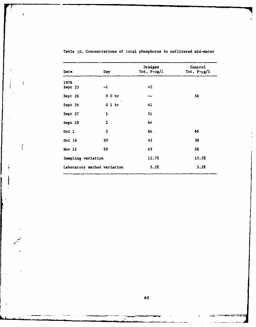
Table 10. Concentrations of total phosphorus in unfiltered mid-water
Dredged ControlDate Day Tot. P-ugh/ Tot. P-ugh/
1978
Sept 25 -1 42
Sept 26 0 0 hr -- 56
Sept 26 0 1 hr 41
Sept 27 1 51
Sept 28 2 64
Oct 1 5 64. 66
Oct 16 20 41 38
Nov 15 50 45 58
Sampling variation 12.7% 15.5%
Laboratory method variation 5.3% 5.3%
40

I
C -' 44o ,, . tW4. .. .
4_ , I .5 o o ,
o -_,
, , ' . '+, . . . ,-
* . 4, -I ii i,
- .444

* 9- ----- mm. -..
-so
IN-
Ik I FP
- u-sOmmopu
-
020
42

concentrations of orthophosphate in filtered interface water four timeshigher than those obtained prior to dredging. This increase was sig-nificantly higher (.05 level) for a period of 20 days following dredging.
The levels of total phosphorus in the particulate material ofunfiltered interface water decreased on dredging. Twenty days later thetotal phosphorus level had recovered, but levels lower than in thecontrols were maintained. For a 50-day period following dredging, themeasurements of Total P at the dredged site were lower than those at thecontrol and were significant at the .025 level (Figures 14 and 15).
Total Kjeldahl Nitrogen
Two days after dredging, the concentration of total Kjeldahl nitrogenin the particulate fraction of interface water had diminished to half ofits original value. By day 5, the level had all but recovered. Fromday 5 to day 20 a second decrease occurred, which constrasted withincreases in the control samples. By day 50 following dredging, increasedlevels were apparent again although still below control levels (Figure 16).
Sediment Analyses
The results of nutrient analyses for sediments are found in Table 12,and Figures 17 and 18. Total phosphorus varied between 0.034 and 0.055%dry weight in both control and dredged sediments. All values of totalKjeldahl nitrogen, whether control or experimental, were in the range of0.017 to 0.303% dry weight of sediment.
Total Phosphorus
The total phosphorus content of the sediments at the dredging sitedropped from 0.055 to 0.037% dry weight with the onset of dredging(dredge outlet sample). Twenty-four hours after dredging began, however,the total phosphorus concentration had returned to close to its originalvalue. A second decrease was apparent through days 2 and 5. Thereafter,while the values remained marginally below those of the control samples,the pattern of behavior of total phosphorus in the dredged sediments didnot deviate from that in the control sediments (Figure 17).
Total Kjeldahl Nitrogen
Of all the nutrients measured, dredging had the most dramatic effecton the total Kjeldahl nitrogen (Total Kj-N) content of the sediments.Before dredging began, the Total Kj-N level was 0.272% dry weight. Theconcentration in the sample taken from the dredge outlet was 0.017%,representing only %5% of the initial nitrogen content of the undredgedsediments. Then began a slow recovery. By day 50 after dredging, thenitrogen content of the sediments exposed to dredging was significantlylower than that of the control sediments at the 0.025 level. By days 205and 233, nir'gen concentrations were still lower in the dredged sediments,at the 0.01 and 0.05 significance levels, respectively (Figure 18).
43

uo P~gswe 14.Ofl~m PGs - "Wed hb.wf VIE
_00 --- Cap"
So-
70
40.0
U --
wo oh form
Plowe I&.A- TOW P - miwn PEOMM
-- can
a -% %%
/
AM-
Will ot n 0.90To IV
j4

W4-
? In
0n %0 en tm
"4
0 0
'A
"4 "
1-1
0 9 m 0 N I 0 CD &4 CON'w C4 "4k A A ' 0 H -A
C4 04 0 4 0In" " 4 "4 p
.0 . .M C6 .; . .A
0h cl 0
0o ta Al 0 e
"45

--- -o a
0 6Th" IDSVW
a- Tam p.
/ %
M-
46

.3
J00 ------------II
47
I- -------

Metals
In the figures of the heavy metal analyses in the sediments at thedredged site, concentration values of the interface particulate materialhave been substituted for sediment values for days 1 and 2 followingdredging. These substitutions were necessary because immediately fol-lowing dredging, it was impossible to distinguish the sediment-waterinterface in the fluid mud sediments at the dredged site.
The analysis of cadmium in the water samples was limited. Thesensitivity of the instrumentation was 0.01 pg/ml, necessitating concen-tration of samples. Although the water samples were heat concentrated,analysis was at the limit of sensitivity. Often no cadmium was registered.Those levels recorded were: filtered and unfiltered mid-water (controland dredged) < 1.5 pg/i; filtered and unfiltered interface water (controland dredged) < 3.5 pg/I; sediments 1.0-3.0 jg/kg.
Iron
Iron concentrations in water and sediment samples are given inTable 13 and Figures 19-23.
Mid-Water Analyses
With the onset of dredging, the concentration of iron in filteredmid-water increased from 100 to 239 pg/l, but within one hour, it haddecreased to 56 pg/i, a value that remained through day 1. By day 2,the concentration of iron in the filtered mid-water at the dredging sitehad increased to values slightly above those obtained before dredgingbegan. By day 20, however, the iron content of filtered mid-water fromthe dredging site did not differ from control values (Figure 19).
When dredging commenced, the concentration of iron in unfilteredmid-water increased from 372 pg/1 to 664 pg/l. The recovery to levelsclose to the original was slower than in filtered mid-water. By day 5,the concentration of iron had dropped to 266 pg/i, a value somewhatbelow that obtained before dredging began. Day 20 showed a secondincrease to 459 pg/i. By day 50, control and experimental values werevery comparable.
For a 50-day period following dredging, the iron content of unfil--" tered mid-water was significantly higher (.05 confidence level) at the
dredged site than at the control site (Figure 20).
Interface Water Analyses
Twenty-four hours after dredging, the iron content of filteredinterface water had decreased to <50 of its initial value. By day 5,the original concentration level was restored and did not vary consider-ably thereafter (Figure 21).
48
-._ . . . .. . . . .

-- p
12it C '
U C
i .-'-....- . .
u4 *
1 "
49A
- t.4 . -
U.~

Plgwe 10.AD-POW" miiw
Ogis 3
no-
9050

FIgWW 21.
go--
I -
11 Sptwou7s 1
swoles
1WM 22
ft INI Pw 51m
I ___a
-. ~~~~~~ %- %
-- ---------
-

The concentration of iron in interface particulate samples was 15.6g/Kg dry weight before dredging. Values of 22.3 and 21.8 g/Kg weremeasured in interface particulate samples from the dredging site days 1and 2 after dredging. Thereafter, the iron content decreased, and byday 50, levels had returned to original values (Figure 22).
Sediment Analyses
Substituting interface particulate for sediment values, it may bethat the iron content of the sediments increased initially in responseto dredging. By day 5 and subsequently, the concentrations of iron indredged sediments did not differ from control values.
Manganese
The results of the manganese analyses in water and sediment samplesare given in Table 14 and Figures 24-28.
Mid-Water Analyses
The onset of dredging produced an extremely large increase in theamount of manganese in filtered mid-water from the dredging site. Avalue of <10 pg/l initially increased to %300 mg/i at the point ofdredging. However, within an hour of dredging activity, the manganeseconcentration had dropped to 113 pg/l, and 24 hours later, the concen-trations of manganese had returned to 5 pg/l (Figure 24).
As happened with iron, dredging caused significant changes inunfiltered mid-water samples. While some recovery took place throughday 5, by days 20 and 50, manganese concentrations in unfiltered mid-water samples at the dredging site were still higher than control valuesat the .025 level of significance (Figure 25).
Interface Water Analyses
Any comparison between control and experimental results for filteredinterface water was difficult. Before dredging began, there was sub-stantially more manganese in filtered interface water at the controlsite. However, the results of the analyses of manganese concentrations
- in filtered interface water at the dredging site showed an initial dropin response to dredging. By days 5 and 20, the concentrations hadlargely recovered (Figure 26).
Unlike iron, the manganese content of the interface particulatematerial decreased following dredging. The initial concentration of1.3 g/Kg decreased to 0.8 g/Kg by day 5. By day 20, the initial concen-tration values had been reestablished, and that situation remainedthrough day 50, possibly indicating a long-term difterence between thetwo sites (Figure 27).
52
-7!

I
N * . , a* .
- -. -, -. N
i.
1U 3
h.E
a",
a- C U"*
! °- "... "
* 5a

tfd~
Can
ao - Iftsm
224
mo
'154

Mp"g. 2&.
Ti ftw ~
140]2
vaPM mf A
IND
mo
55

4=oo Flom 27.
I"39 - - Comm
/I/
/lloI "I I
/I 'Iuw-
U /
2W I
I'
0--..
Fop" 2&.
C"
0
IIkl. i
Ii.,In,
eW 2% aOt u N"M AV 1
56

Sediment Analyses
It would seem that some decrease sediment manganese occurred initially,at least through day 5. By day 20, the concentration of manganese inthe dredged sediments was essentially equivalent to the before-dredginglevel but remained lower than control (Figure 28). This situation wassimilar to interface samples.
Lead
The results of the measurement of lead concentrations in water andsediment samples are given in Table 15 and Figures 29-33.
Hid-Water Analyses
The lead content of filtered mid-water increased from 25 to 110pg/l with the onset of dredging. The higher values were maintained fora period of two days. By day 5 the level had dropped to 13 pg/l, somewhatbelow the initial value of 25 pg/l. A second increase to 50 jjg/l wasmeasured on day 20. The second higher value was still apparent onday 50 (Figure 29).
In response to dredging, the lead content of unfiltered mid-waterincreased from 36 pg/1 before dredging to 66 pg/i 2 days after dredging.However, the concentration of lead in control samples varied greatly(9 - 95 pg/l), which reduced the significance of effects due to dredging(Figure 30).
* Interface Water Analyses
Before dredging began, the concentrations of lead in filteredinterface water at the dredging site were much below those at the controlsite, 9 pg/l and 27 pg/l, respectively. However, lead values in theexperimental samples showed incLeases during a 5 day period subsequentto dredging, when control values exhibited decreases (Figure 31).
The concentration of lead in the interface particulate material in-creased from 32.3 to 47.4 mg/Kg by day 1 following dredging. It thendecreased: values on days 2 and 5 were 35.6 mg/Kg and 21.5 mg/Kg,
*respectively. A second increase was measured on day 20, associated withan increase in control values. By day 50, experimental and control
-" values were equivalent (Figure 32).
Sediment Analyses
Using substituted interface particulate values for sediment values,the effect of dredging on the lead content of sediments appears to havebeen minimal. Apart from a small initial increase on day 1 followingdredging, the concentrations of lead in dredged and control sedimentswere similar (Figure 33).
57
----S
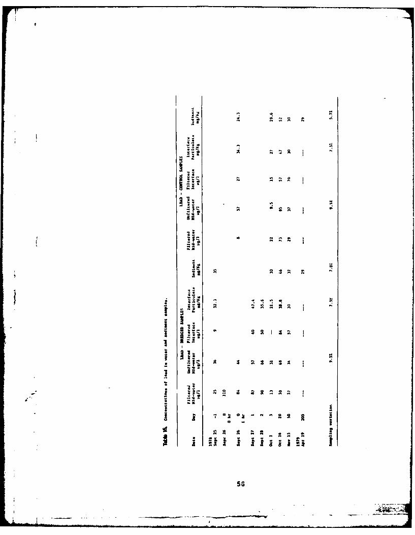
4 ~ z' 0
1
k.
t 3: to, 4 '
~go-
- a- W

US-i ig,. 2LPb - PUIud MwWr
100
25-
I s sau om 5 J201
100-PFla" 30.Pb * iMOWNW Mkk.
70-
"Si
Iu.20
- J40 tIh Mo
I 59

Flgwe 31.
go-i-0
1.0-i
.0-
U0
m-k
hp* 33L
I'*M~nPod
% J
5 / If go
60
Zinc
Zinc results are found in Table 16 and Figures 34-38. Dredging hadno measurable effect on the concentrations of zinc in water and sedimentsamples.
Mid-Water Analyses
The isolated abnormally high value of 175 pg/l in filtered mid-wateron day 50 following dredging must be noted and could be attributed tohighly localized and temporary contamination present in the surfacewater at the dredging site. This value has been excluded from averaging.
In filtered mid-water, the average concentrations of zinc at thecontrol and dredging sites were equivalent (34 pg/1) for a period of50 days following dredging activity (Figure 34). Similarly, the averageconcentrations of zinc in unfiltered mid-water samples were essentiallyequivalent at the control and dredging site over the same period, being23.7 and 22.8 pg/i, respectively (Figure 35).
Interface Water Analyses
The similarity between control and experimental values continued ininterface water; average concentrations in filtered interface water were36 pg/i at the dredged site over 50 days and 40.2 pg/l at the controlsite (Figure 36). For the same period, the average zinc content of theinterface particulate material was 70.1 mg/Kg at the dredging site and72.0 mg/Kg at the control site (Figure 37).
Sediment Analyses
When results for the zinc content of interface particulate materialwere substituted for sediment values, the average zinc content of sedi-ments at the dredging site was 65.3 mg/Kg, compared with 70.4 at thecontrol site (Figure 38).
Copper
The results of the analyses for copper in water and sediment samples--are given in Table 17 and Figures 39-43.
As was the case with zinc, there was no indication of a dredgingeffect on the concentrations of copper in the water and sediments at thedredging site. Average concentrations of copper in control and experi-mental samples varied little, if at all. In filtered mid-water, theaverage control and experimental concentrations of copper over 50 dayswere 10.5 pg/1 and 12.3 pg/l, respectively; in unfiltered mid-water,12.7 pg/1 and 11.0 pg/i; in filtered interface water, 13.0 pg/l and13.7 pg/i; in interface particulate samples, 25.9 mg/Kg and 23.6 mg/Kg;in sediment samples, the values were 22.8 mg/Kg and 24.1 mg/Kg, respec-tively.
61
- - - - - - -•

i~AA
go 0:
-1w-

Plip~Me 33.
go -Cd
20
i a 0 2 s o%08 m TIM W Apr IA
uo-
40 O
0 j6'we O103 I@OS I
TkwMu
63

Ftgive 35.
3 61 ~ ~~z - W 'I U I V M d M u k w - r
30-
Is-
P~26 55.Im l 2 act 1111 "M III
Th" MM
-w"34
U -1 I
0-.
weO 6 lt0 "M
64

Flows 37.Za himt~ PWVUImb
70-
% V
*1 0 36 U
100-
Flowse 3L
90 Ondeed.
oo - CAN"
I0
65

-t
Vi - A-A A A C C
S. - - .4 -
5-3-- SW
-tt .40 A.4"-' I
A C * A
- - - I
8~i I
I.,A '48 ~ C U A
-- -,a I -
'a.S.
A C I*.
-'a a IS.C
1:-~ ... * .4 A C'iv - - 'a .4 -
VI
S
0~
A*L. -- UM .4
- - - .4 - C A g.4 .4 .4 .4 .4 - .4~A1i' ~0~~ -, I
.-
U
~i-I.- - ** .3 .3A - .4 *3 4~ A
- - - -
o U'a.
-~ ~ ~ I- - 'a.* VI
S.C
- 1 .1OO - .4 A @~
a a A* -SS
A A 'A - - I~ ~ .4 .4 A A A Ak - I
66

- Plqwo 39.
SC -- Mnd
Is-
10*
Is.I a. asU~
~. s~aOgalS
im u w
a67

Flw 41.
20 --- Can"
Is-
10-
- -- n
( 0- J 6U
we San orsm
6-8

20-
10
wes -36r o' s s e10
sw n oo in "M -- or 1
J7s
69

Discussion
Nutrients
+ It would seem more realistic to comment only on the behavior of(NH4)-N in mid-water following dredging for a 50 day period because ofthe time gap between days 50 and 259.
Examination of Figre 8 shows that, apart from the immediate risein concentration of (NH4)-N in response to dredging, the variations inthe concentration in mid-water at the dredged site were parallel tosimilar behavior at the control station, but at much lower levels. Thiswould suggest that the sediments that were redeposited following dredgingresponded more easily than csntrol sediments to environmental factorspromoting the release of (NH4)-N.
Day 20, October 16, 1978, together with October 14 and 15, experi-enced the highest winds (15-17 mph) of the entire 50-day period. Thehigh wind values were associated with increases in the (NH4)-N concen-trations in dredged and control mid-water samples, but the dredgedconcentration were ^20 pg/l higher than the controls.
During hydraulic shell dredging, large volumes of anaerobic sedimentsfrom depth are gouged from the lake bottom and redeposited in the imme-diate vicinity as a dispersed slurry. The deposition of anaerobic+sediments containing inorganic nitrogen in the reluced form as (N14)-Non the lake bottom can account for the higher (NH4)-N concentrations inthe mid-water at the dredged site.
Dredging alters the physical characteristics of the sediments.They are redeposited with a fluffy consistency and are much less consoli-dated than control sediments for a lengthy period following their deposi-tion. As can be seen from other sections of this report, low bulkdensity dredged sediments were deposited over a wide area at the dredgedstation. The lack of consolidation and the decrease in bulk density ofanaerobic sedimegts redeposited after dredging would facilitate thediffusion of (NH4)-N through the interstitial water, making it availableto the overlying mid-water.
The total inorganic nitrogen values, found to be significantlyhigher at the dredging site over 50 days, can be explained similarly.The oxidized nitrogen fraction (NO; + NO2 ) of the total inorganic nitro-gen content of mid-water did not alter in response to dredging over theperiod from day -1 to day 50. In samples from the dredging site, the(NO; + NO;) component of the total inorganic nitrogen was 33.41, theaverage value over 50 days. In control samples, the (NO3 + NO2) contentaveraged 34.1% of the total inorganic nitrogen. The significantlyhigher values of total inorganic nitrogen in mid-water for 50 daysfollowing dredging must $hen be related directly to the significantincreases in reduced (Nil4) nitrogen.
The initial increases in orthophosphate and total phosphorus inmid-water samples for 2-5 days following dredging are considered to be
70
attributable to the interaction of the reduced sediments with the watercolumn. Orthophosphate was released into solution from the reducedsediments in contact with the water column during disposal and resedi-mentation. The increased amounts of total phosphorus in mid-watersamples over 2-5 days following dredging were associated with increasedamounts of particulate material in resuspension in the water.
When the results obtained for (NH4)-N concentrations in interfacewatsr are compared with mid-water values, trends are apparent. The(NH )-N concentrations in filtered interface water increased initiallyupon dredging and then decreased to levels comparable with those of thecontrol, but always 10-20 pg/l higher. Again, it would seem that thechanges in the physical characteristics of the dredged sediments facili-tated diffusion of (NH4)-N through the less consolidated anaerobicsediments, thus increasing the (NH4)-N content of interface water.
As happened with mid-water, the (NO; + NO;) fraction of total inor-ganic nitrogen in filtered interface was roughly equivalent in dredgedand control samples, being 39% and 35%, respectively. It can be assumedthat the higher values of total inorganic nitrogen found in dregged samplesover 20 days following dredging were caused by increases in (NH4)-N.
At the interface, significantly higher amounts of orthophosphate infiltered water were associated with decreases in the total phosphoruscontent of the particulate fraction. It would seem, therefore, that theremoval of reduced sediments from depth by dredging and their superficialredeposition on the lake bottom promoted the release of soluble ortho-phosphate from the particulate fraction into the water. The decrease inthe total phosphorus content of the particulate fraction was probablydue in part to the removal of orthophosphate into solution. The deepsediments redistributed at the interface would be expected to containless organic matter and hence less measurable total phosphorus.
Lower amounts of organic matter would also be associated with lowe-values of total Kjeldahl nitrogen in the particulate material of theinterface water.
Samples of the slurry from the dredge outlet showed a 33% reductionin total phosphorus, reflecting the lower organic content of the deepersediments redistributed at the interface by dredging activity.
The slurry from the dredge contained only 5% of the total Kjeldahlnitrogen of undredged sediments. There was, however, a gradual increase inthe total Kjeldahl nitrogen of the redeposited sediments for a period of9 months following dredging. The increase accompanies the presumed accumu-lation of organic plant and animal debris at the water/sediment interface.
Summary
Nutrients
It can be concluded that hydraulic shell dredging had significanteffects on the nutrient chemistry of the waters and sediments of LakePontchartrain.
71
A-..- o1

The response of nitrogen nutrients to dredging was demonstratedover a lengthy period of 9 months. The ammonia nitrogen content ofshallow water maintained a significant increase over control samples.The total Kjeldahl nitrogen content of the dredge slurry was only 5% ofthe sediments before disturbance by dredging. Thereafter, the organicnitrogen content recovered with time.
For a period of 50 days following dredging, the balance of phosphorusexhibited changes. At the water/sediment interface, soluble inorganicphosphate in filtered water was present in increased amounts. The totalphosphorus content of the particulate fraction of interface water showeda decrease.
It is thought also that the dredging activity altered the physicalcharacteristics of the sediments, rendering t~em more sensitive toenvironmental stresses. The diffusion of (NH4)-N through the redepositedsediments was facilitated. Also, the redeposited material that originateddeep within the sediments had lower values of total phosphorus and totalKjeldahl nitrogen than did sediment samples undisturbed by dredging.
Metals
The analytical results indicate that copper and zinc concentrationsin water and sediments are not affected by dredging. This non-effect isin keeping with Gorham and Swaine (1965) and May (1973). However, filteredinterface water concentrations of lead, zinc, and copper appear to beelevated after dredging.
The observed variations in the levels of iron and manganese inunfiltered mid-water suggest that dredging activity has a substantialand lasting effect on the concentration of these two metals. That sucheffects are not significant statistically in interface water or sedimentsindicates that the iron and manganese concentrations are related toartificial suspension induced by dredging.
The initial, immediate, high values of iron and manganese in mid-water may be due to the suspension of reduced hydrous oxides of iron andmanganese derived from the bottom sediments and redischarged into thewater column. In unfiltered mid-water samples, the decrease that occursover 5 days following the initial increase can be attributed to slowsettlement of fine particulate material.
The fast recovery of iron and manganese concentrations in filtered-" mid-water within 24 hours following dredging is noteworthy. It is
thought that the fast recovery from the immediate high values may be dueto the chemical reactions of these metals in response to the temporaryaeration of the dredging activity.
Many workers (Mortimer 1971, Lee 1975, Gotoh and Patrick 1972,Patrick et al. 1977) have found that the oxidation-reduction potentialof surface waters and sediments regulates the concentrations of iron andmanganese and their bioavailability in water-sediment systems. Inanaerobic conditions, soluble-reduced forms of these metals predominate;
72

in the presence of dissolved oxygen, insoluble oxidized compounds ofiron and manganese are formed.
The sudden change in oxidation-reduction conditions accompanyinghydraulic shell dredging in Lake Pontchartrain means that reduced ironand manganese compounds may be converted to insoluble oxidized forms.The immediate increase and fast recovery of the concentrations of thesetwo metals in filtered mid-water could be accounted for in these terms.Soluble, reduced iron and manganese oxides, which are imediateiy detect-able in filtered water, will remain as fine suspensions of insolubleferric and manganese precipitates, which settle more siowly,. and areonly measurable in unfiltered samples.
The secondary increases in the iron and manganese levels in unfil-tered mid-water in association with 15-17 mph winds that occurred justbefore and during day 20 can be attributed to two factors. Wave-inducedreoxygenation of the water column combines with the greater susceptibilityof redeposited dredged sediments to entrainment by wave-induced forces.The concentration distribution through the 50 day sampling period,therefore, reflects both the initial effect of dredging and subsequentstorm effects.
Conclusions
It can be concluded that hydraulic shell dredging had significanteffects on the nutrient and heavy metal chemistry of the water andsediments of Lake Pontchartrain.
Dredging augmented significantly the amounts of ammonia nitrogenand soluble phosphate in the water column at the dredging site. Also,the total phosphorus content of interface particulate material decreasedsignificantly in response to dredging, asdid the total Kjeldahl nitrogencontent of the dredged and redeposited sediments.
The iron content of unfiltered mid-water at the dredging siteremained significantly higher than that of control samples (.05 level)for a 50-day period. It is suggested that these higher iron values arein part due to the artificial resuspension of sediments and to the slowsettlement of very fine particulate material following dredging. Thechange in the physical properties of the redeposited sediments alsoincreased their sensitivity to subsequent wind and wave effects.
The manganese content of unfiltered mid-water reacted to the dredgingsimilarly to iron. Significantly higher values of manganese (.025level) were in evidence at the dredged site over a period of 50 days.
No significant dredging effects were measured on the concentrationsof lead, zinc, and copper.
73

EFFECTS OF SHELL DREDGING ON THE BENTHICFAUNA OF LAKE PONTCHARTRAIN
Introduction
Since Lake Pontchartrain is quite shallow, averaging 4 m over mostof the central portion of the lake, there is a much smaller ratio ofwater volume to bottom area than in other large lakes or in, for instance,the open gulf. Consequently, the benthic food web is considerably moreimportant than in many other aquatic systems. Many of the dominant fishspecies such as the spot, Leiostomus xanthurus Lacepede, or the Atlanticcroaker, Micropogonius undulatus (Linnaeus), feed on the benthic inverte-brates (Levine 1980) as do many of the migrant waterfowl of the area,for instance the Lesser scaup, Aythya affinis (Eyton), and the Greaterscaup, Aythya marila (Linnaeus). Thus any assessment of the impact ofman's activities on the lake ecosystem should include a careful analysisof the impact on the benthos.
Methods
To quantitatively assess the impact of hydraulic shell dredging onthe benthic fauna of Lake Pontchartrain, a series of replicate quantita-tive samples at the experimentally dredged site and the nearby controlsite were taken with a modified J&O box corer (Jonassen and Olausson1966) 0.09 M2 and subsampled with acrylic core tubes (4.9 cm2) formeiofauna samples. Any box corer sample that appeared to be disturbed(such as when rough water would cause the boat to move enough to causethe corer to enter the sediment at an angle instead of straight down),that appeared to 'have entered the sediment too deeply so that organismscould be lost through the top, or that appeared to be leaking in anyamount because of a piece of shell preventing full closure of the jawsof the device, were discarded. The contents of the box corer weresieved first through a one-half inch (1.27 cm) mesh, then one-eighthinch (0.32 cm) mesh to remove large shells and organisms, then through a0.5 m screen to retain the remainder of the macrofauna (animals > 500 pm).All fractions were preserved onboard ship in a buffered formalin solutionwith Rose Bengal stain. Meiofauna samples (animals between 500 and44 pm) were preserved unsieved. All samples were returned to the labora-tory for further sieving, enumeration, identification, and archiving.Organisms were identified to the lowest practical taxon, with certainforms being sent to specialists for confirmation, or further identifica-tion.
-" Heiofauna samples were sieved in the laboratory through a series ofsieves. Animals retained on the 500 pm sieve were returned to themacrofauna sample from the box core from which the meiofauna core wasremoved. Animals retained on the 63 pm and 44 pm sieves were counted asm.,iofauna. As animals were identified, they were placed in appropriatelylabelled vials. All vials were recounted by another person, and theresidue from which the animals had been removed was searched for animalsthat might have been overlooked. No sorter was retained whose accuracyhad not improved to better than 95% by the third sample. After a sorter
74
I ... . . ... ... . .. I . . .-

t
had improved to better than 97%, only every third sample was checked.By recounting all vials of new sorters, and rechecking residues, totalsorter error for the laboratory for meiofauna was held to under 3%.Sample vials have been archived for further use by taxonomic specialistsif requested.
All macrofauna sorted to major taxa by student workers were identi-fied to species by the more highly trained technical staff. Some specimenswere sent to consulting taxonomic specialists for confirmation of identifi-cation. Some undescribed species are listed as such. Since macrofaunaare rechecked as species identifications are made, the additional re-counting to maintain laboratory efficiency in meiofauna sorting is notnecessary for macrofauna sorting.
Samples at the experimentally dredged site were taken initially,before dredging, and on days 1, 2, 5, 20, 50, 205, 235, and 331. Thecontrol site was sampled initially and then on days 5, 20, 50, 205, 235,and 331. After the first year, samples have been taken at the two studysites quarterly. A total of 104 meiofauna and 78 macrofauna sampleshave been completed and analyzed to this date.
Standard statistical analyses were performed using standard programs;certain special programs for classification and ordination of benthicdata were provided by Dr. Stephen A. Bloom of the University of Florida(Bloom et al. 1977). No transformations of the data were used. Toprevent the classification from being unduly biased by large numbers,(dominant species) or small numbers (rare species), a simultaneousdouble standardization was used (Boesch 1973). The Canberra metric wasused as a measure of dissimilarity, with a flexible sorting strategy( = -0.25), to produce the clusters for the analysis (Boesch 1977).
Results
Abundance of Meiofauna
Examination of the meiofauna community (Table 18, Table Bi, andFigure 44) shows first that there were fewer animals at the experimentalsite than at the control site originally, before the experimental dredgingwas done. The numbers of true meiofauna, such as nematodes and copepods,were not significantly different. The major differences occurred informs such as ostracods and bivalves that could settle out of the plankton.
- This patchiness in species settling is a common phenomenon, accountingfor a great deal of the natural fluctuations in both the macrofaunal andmeiofaunal components of soft-bottom benthic comuunities (Eagle 1975).The day after dredging, the abundance at the dredging site had droppedto approximately half its previous value. This is accounted for bynoting that although very few nematodes came through the dredge outletin recognizable form, dredging at the experimental site in a typical"soft-bottom," or light silt-clay, left a series of troughs and ridgesthat, through slumping, coalesced, and thus redistributed the animalsremaining in the ridge of undredged areas of the experimental site overthe entire area. The second day after dredging, the abundance of total
75

Table 18. Meiofauna, major components
Experimental Control
N110 cm 2SE N/10 cm2 SE
-------------- Initial--------------- ----
Nematodes 228.7 20.9 288.8 21.4*Copepods 68.8 10.9 94.2 7.0
Others 242.9 279.6TOTAL 540.4 10.9 662.6 43.4
---------------- Day 1 --- ------------
Nematodes 104.9 49.4Copepods 33.6 6.7Others 124.8TOTAL 263.3 47.1
----------------- - ----------------- --------- Day 2- ------- ---------
Nematodes 167.6 41.8Copepods 19.4 4.6(Others 252.11TOTAL 439.0 81.8
---------- - ---- Day 5--- - --------------
Nematodes 151.3 12.9 196.1 55.2Copepods 13.2 3.6 26.5 9.0OTHERS 165.0 205.2TOTAL - 329.5 -- - - - 30.0 - - Da 20 427.8 -- - - - - 119.9 - -
------------------------------------Da2 -----------------
Nematodes 47.4 12.9 173.2 31.6Copepods 26.5 8.6 34.6 6.6Others 78.9 198.1 7.TOTAL 152.8 42.4 405.9 7.
--- --- ------------ Day 50 - --------
Nematodes 234.3 20.3 457.4 77.6Copepods 37.2 5.S 68.3 6.7Other 276.5 278.5TOTAL 548.0 38.5 803.7 161.0
-------------- Day 205-----------------
*Nematodes 264.9 52.8 592.6 44.0Copepods 108.0 25.2 58.8 13.9
*Others 246.4 167.3TOTAL 609.6 76.9 720.7 131.5
* I 76

Table 18. (Continued)
Experimental Control
N/10 cm2 SE N/10 cm2 SE
---------------------- Day 235------------------------
Nematodes 324.4 60.2 712.0 43.7Copepods 40.7 7.3 81.5 5.3Others 152.3 301.5TOTAL 517.4 83.4 1,094.1 41.3
------------------------- Aug 79------------------------
Nematodes 202.7 30.4 238.0 94.9Copepods 151.8 21.0 56.9 13.0Others 198.1 626.4TOTAL 552.6 53.8 921.3 85.4
- - ---- - --- Nov 79 - -- - - -
Nematodes 352.9 36.3 266.4 37.2Copepods 83.5 8.2 108.5 20.6Others 215.5 131.9TOTAL 651.9 87.7 506.8 73.6
----------- ----- Feb 80 -------- -
Nematodes 480.3 81.5 648.4 126.0Copepods 174.2 61.7 112.1 9.7Others 169.0 331.4TOTAL 823.5 64.1 1,091.9 115.6
------------------------- May 80 ------------
Nematodes 644.3 86.0 857.7 129.7Copepods 65.2 19.9 35.1 7.7Others 125.8 192.0TOTAL 835.3 85.9 1,084.8 95.8
------------------------- Aug 80--------------
Nematodes 529.2 115.9 377.4 20.9Copepods 70.3 19.1 58.1 6.5Others 442.0 381.5TOTAL 1,041.5 173.4 817.0 52.8
------------------------- Dec 80
Nematodes 1,242.2 163.9 1,278.3 163.1Copepods 94.2 10.9 60.6 8.5Others 357.0 284.2TOTAL 1,693.4 197.1 1,623.1 199.0
77
NM

AU
.410 o
P.4
go
s=01/N
78.
i1
meiofauna at the experimental site was higher because of another settle-ment of very small (< 500 pm) bivalves and influx of ostracods, in aboutthe same numbers that the control site had received them a few dayspreviously.
By the 20th day, abundance at both sites fell, possibly a seasonaleffect, with the numbers at the experimental site becoming significantlylower than at the control site. This difference was maintained throughthe 50th and 200th day samples, becoming more pronounced by the 235thday samples, when the control site had twice as many animals as theexperimental, a quite significant difference. Analysis of the Augustdata shows that this difference was maintained throughout the summer ofthe first year.
During the second year of the study, abundance of meiofauna declinedduring the fall months at the control site and increased at the experi-mental site, with the result that the November 1979 samples are notsignificantly different at the two study sites. Heiofauna at the controlsite increased more rapidly during the winter, with the differencesbetween the two sites reappearing. Both the February 1980 and the May1980 samples from the experimental site are about 75% of the density ofthe control site. These differences are not as great as the previousyear, when the experimental site was only 47% of the control (in ay1979). In August 1980, concurrent with the sharp decrease in the densityof animals at several of the benthic characterization study sites, areduction occurred in the density of the meiofauna at the control site,with an increase at the experimental site.
Integration over time of the average daily standing stock of meio-fauna at the two study sites to obtain a mean daily value for the firstyear showed the experimental site to be significantly lower, at 528.67/10 cM2, than the control site, at 841.01/10 cm2 .
Integrating the second year's data similarly, the experimental siteremains somewhat lower, with 774.83/10 cm2 , than the control site, with885.75/10 cm2 . This difference in the average daily standing stock forthe second year is not significant (P S 0.05).
Samples taken during December 1980 at the beginning of the thirdyear of the study show very high densities of meiofauna at both thestudy sites. The abundance of 1693.4/10 cm2 at the experimental site isnot significantly different from the abundance of 1623.1/10 cm2 at thecontrol site. It is, however, significantly higher than 97% of themeiofauna samples taken in Lake Pontchartrain during the course of thetwo concurrent studies. Fluctuations of this magnitude are not uncommonin benthic studies. Coull and Bell (1979) describe a station where overthe course of 63 months of sampling, the density varied by over an orderof magnitude.
It is possible that if the study sites were sampled in ay 1981(the time of the year when differences have been most pronounced), theymay not be significantly different. Because of their very small sizeand the importance of the size to volume ratio, the meiofauna have thebest chance of surviving in the sediments that have been altered bydredging.
79
* -----mm nmmnm-- -- h. ..... ' .. . . .- .. . . .. . . . . ". .

An examination of the patterns of abundance in the nematodes(Figure 45) shows more clearly the actual dynamics at the two sites.There are no significant differences at the experimental and the controlsites before the experimental dredging. After the fifth day, the dif-ferences are significant and remain so until the end of the first year.Patterns for the second year are quite similar to that of the totalmeiofauna.
Abundance of Hacrofauna
An examination of the changes in the abundance of macrofauna foundat the two study sites (Figure 46, Table 19, and Table B2) reveals acomplex pattern. Initial macrofaunal numbers were not significantlydifferent at the control site and the experimentally dredged site. Bythe second day after the dredging, the numbers of animals at the exper-imental site were reduced to 54% of the initial numbers. A settlementof the two small gastropods Probythinella louisianae and Texadinasphinctostoma caused a considerable increase in the numbers by the fifthday. These animals did not appear to survive well in the altered sedimentsand by day 20, the numbers had fallen again. Further settlement ofsmall molluscs at day 50 again increased the total numbers, but byday 205, the experimental site was reduced to 54 of the numbers at thecontrol site.
After the opening and subsequent closing of the Bonnet Carri Spill-way into Lake Pontchartrain, the two study sites were sampled again(day 235, Hay 1979), and total population at the experimental site haddropped further, to 38 of the control site. We can only speculateabout this additional drop in benthic community numbers. It is possiblethat the additional stress of the rapid change in salinity and watertemperatures at the study site resulting from the opening of the BonnetICarri Spillway caused the change in the numbers at the experimentalsite, which was already stressed by the effects of the experimentaldredging. It is also possible that the numbers would have droppedwhether the Spillway was opened or not.
In August 1979 at the end of the first year after dredging, theexperimental site had only 40.7 of the total numbers of animals thatwere present initially. The control site had more than twice as manyanimals present as the experimental site and was not significantlydifferent from initial values.
In November of 1979 a settlement of small gastropods occurredagain, with the total numbers at the two study sites again not signifi-cantly different. By May 1980 the two sites were again different; theexperimental site was reduced to 50.3 of the control site. Figure 47shows the macrofauna divided into two fractions: gastropods and non-gastropods. The gastropod fraction ranged in percent of total animalsfrom 62 to 98, with the overall mean for 78 observations being 86.1.The non-gastropod fraction includes both the bivalves, which make up11.51, and the non-mollusc fauna, which make up only 2.42%, of thetotal, with the chironomid larvae accounting for 1.16% of the total, oralmost half of the non-mollusc fauna. Figure 47 illustrates one of the
so

w
600
41
-4
U) 4A
Si
v~w~l/N

I
a 0U
z.1
00
0'-4U
'4.9.4 hi
I- I..'
.0hi
1 0
I -~ "~ '4________ * 00
00* 0 4.h.jJ
I I 00
I I -@8 / 2
Ii~
-~ 000
-~ U00.044'.
Z 0'.~400
0 CU'40"'a
0 00Ciba
@0.0$4
.0
I 44
I *' 0
-7.---p .11~
2 IC:0 '4400
if - -~ I00
2 2 2 2 2 9 2 aaW/SUNVSflOHJ.
82
-------- - - - -~ -

-ITTable 19. Macrofauna, major components
Experimental Control
N/M2 SE % NI/ 2 SE z
Initial
Bivalves 4,766 173 11.4 3,743 105 9.9Gastropods 36,534 746 87.0 33,284 581 88.4Non-mollusc 683 43 1.6 664 85 1.7TOTAL 42,013 607 37,660 477
Day 1
Bivalves 4,825 1,355 12.5Gastropods 33,223 2,617 86.5Non-mollusc 378 155 1.0TOTAL 38,426 3,811
Day 2
Bivalves 1,569 460 6.9Gastropods 20,616 12,769 90.9Non-mollusc 505 79 2.2TOTAL 22,689 13,310
- - Day 5
Bivalves 2,197 767 4.1 4,274 774 9.3Gastropods 50,633 14,524 94.2 40,927 9,606 89.2Non-mollusc 911 237 1.7 72 168 1.5TOTAL 53,741 15,211 45,873 10,318
Day 20 . - -
Bivalves 1,009 868 8.4 2,988 388 8.2Gastropods 10,559 3,073 87.8 32,765 50 89.9Non-mollusc 457 137 3.8 686 64 1.9TOTAL 12,026 3,873 36,440 369
Day 50
Bivalves 4,749 1,938 11.8 2,701 252 7.2* Gaecropda 33,698 12,816 84.1 33,419 11,083 89.5
Non-mollusc 1,641 266 4.1 1,227 93 3.3TOTAL 40,089 14,730 37,347 11,125
Day 200 ,
Bivalves 8,413 3,848 31.0 9,101 997 18.0Gastropods 17,461 10,866 64.2 40,586 436 80.4Non-mollusc 1,307 384 4.8 790 125 1.6TOTAL 27,181 15,021 50,477 1,557
83
- - --,- - *
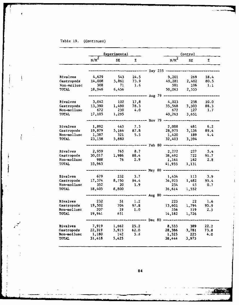
Table 19. (Continued)
Experimental Control
N/M2 SE N/M2 SE
-------------------------- Day 235-------------------------
Bivalves 4,629 543 24.5 9,201 269 18.4Gastropods 14,008 5,861 73.9 40,281 2,402 80.5Non-mollusc 308 71 1.6 581 106 1.1TOTAL 18,946 6,456 50,063 2,555
--------------------------- Aug 79--------------------------
Bivalves 3,042 102 17,8 4,023 258 10.0Gastropods 13,390 1,490 78.3 35,568 3,303 88.3Non-mollusc 672 230 4.0 672 127 1.7TOTAL 17,105 1,295 40,263 3,651
------------------------ Nov 79 ------------------Bivalves 1,892 443 7.5 2,008 481 6.2Gastropods 19,879 5,164 87.8 28,975 3,136 89.4Non-mollusc 1,387 321 5.5 1,420 189 4.4TOTAL 23,158 5,880 32,403 3,394
------------------------------ Feb 80-------------------------
Bivalves 2,959 765 8.7 2,272 227 5.4Gastropods 30,017 1,986 88.4 38,492 722 91.7Non-mollusc 988 76 2.9 1,161 162 2.8TOTAL 33,963 41,955 1,131
----------------------- May 80 --------------------
Bivalves 679 232 3.7 1,434 113 3.9Gastropods 17,374 8,750 94.4 34,925 1,482 95.4Non-mollusc 352 20 1.9 254 45 0.7TOTAL 18,405 8,800 36,614 1,552
-------------------------- ---- Aug 80-------------------
Bivalves 232 51 1.2 225 22 1.6Gastropods 19,502 704 97.8 13,601 1,794 95.9Non-mollusc 207 19 1.0 356 119 2.5TOTAL 19,941 651 14,182 1,726
-------- --------------- Dec 80- --------------
Ij" Bivalves 7,919 1,662 25.2 8,533 389 22.2Gastropods 22,319 3,915 62.0 28,386 3,781 73.8Non-mollusc 1,180 142 3.8 1,525 225 4.0TOTAL 31,418 5,425 38,444 3,975
84

-4t
I~$ 4.4.
I 0 0Sco 0
I0 0 4
4
/ 4.0
0 too 0
tI '"1' 14
a r a1. eI
'I 4 lugw w 4
Ia *' gc
* ~ 0 $.0
o 4 041
Ar40
400
Ga
S a 20
UW/SlugflO00
85 0

AD-A127 189 ENVIRONMENTAL EFFEC S. OF HYDRAULIC DREDGING OR CLAM I/LSHLSI AEPNC OIIN TT NV1 TROUGE COASTAL ECOLOGY LAB WBSIKORAET AL JUN 8
UCAEDhSUCE-8-1mhhhhhmmu09 FG /1NmhhEEmhhmhoh
mhhhEEmhhhImmEl

T
11111 1.0 J 28
liii .1 1 0 f
IIIIL IIII 1111.6
MICROCOPY RESOLUTION TEST CHARTNATIONAL BUREAU OF STANDARDS-_I 96-A

unique features of the Lake Pontchartrain benthic fauna: the very highdominance of the gastropod fraction. The non-gastropod fauna were notsignificantly different at the two study sites except immediately follow-ing the dredging of the experimental site and again in May 1979, followingthe opening and closing of the Bonnet Carrg Spillway.
In May 1980 the non-gastropod fauna were not significantly differentat the two sites, but they comprised only 5% of the total numbers. InAugust 1980 the control site numbers were significantly lowered, to35.2% of the total numbers for the previous August. At no time duringthe course of the study preceding that month had numbers at the controlsite ever fallen so low. This occurred at the same time that stations afew miles to the south and east of the control site had been found,during the course of the concurrent benthic characterization study, tohave had their populations decimated. This finding would lead to theconclusion that this sudden decrease is not a normal seasonal event butthe result of some as yet undiscovered stress to the lake, possibly anintroduction of halogenated hydrocarbons, which were found in significantamounts at the stations south and east of the control site. By December1980 the control site had regained its previous density of organisms andagain, like in November 1978 and November 1979, the two study sites werenot significantly different.
Integration over time of the average daily standing stock to obtaina mean value for the year, i.e., including the time between samplingdates, showed the two study sites to be significantly different thefirst year of the study, with a mean for the control site of 44,059organisms, and for the experimental site, a mean of 27,480. Integrationof the average daily standing stock during the second year of the studyshowed a lowered mean for the control site, 34,274, and also a loweredmean for experimentally dredged site, 23,512. The second year showedonly a 6.2% improvement in the dredged site over the first year. Itwill not be possible to assess the degree to which the experimentallydredged site will recover until after May 1981, because this is the timewhen the two study sites have shown the greatest differences. If atthat time the two sites are shown to be not significantly different,then the experimental site could be considered to have recovered.
Species Diversity
In addition to measures of abundance, certain aspects of communitystructure were measured. Diversity of all collections was measuredusing the Shannon-Wiener index, H' = -1p.loge p.. The diversity of a com-munity depends on two things: the number of sbecies and the evennesswith which the individuals are distributed among them (Pielou 1975). Acommunity with a few, evenly distributed species can have the samediversity as one with many, unevenly represented species. It is there-fore useful to examine not only the diversity of the collections at thetwo study sites but also the evenness and species numbers. Evenness wasmeasured using J' = H'max' where Hmax = log eS, or V = H'/log eS.
Several groups were not identified to species. Chironomids arelumped, for instance, and treated as one species, although an examination
86

by an expert of all specimens collected in the two concurrent studiesshowed more than 99% of Ablabesmyia sp. and less than 1% of Cryto-chironomus sp. and Coelotanypus sp. The nemerteans all belong to oneundescribed species. The number of species of oligochaetes and ostracodshas not yet been completely determined. Since these groups each contributeonly a tenth of one percent to the total numbers and occur in less thana fourth of the samples, it is not likely that the lumping will bias theresults to any significant degree.
Each value given for diversity, evenness, and species number (Table 20)is expressed as the mean and standard error of the measurements made onthe samples collected at each study site on each date.
The initial samples taken at the control site and the experimentallydredged site were not significantly different (P S 0.05) in diversity,in evenness, or in species number. The mean values for diversity, forevenness, and for species numbers at the two study sties are not signif-icantly different (P S 0.05). Differences do arise during the course ofthe study. At day 205, for instance, the macrofauna abundance at thecontrol site is almost double that at the experimental site, yet thediversity at the experimental site is significantly higher. This isprincipally caused by the higher evenness at the experimental site,which in turn is caused by the lower numbers of the two dominant species,the gastropods (Figure 47, Table 19).
Numerical Analysis
The results of the numerical analysip (Bloom et al. 1977) using theclassification produced by the normal analysis of the macrofauna data(Figure 48) are influenced by the fact that the Canberra Metric dissimi-larity measure was chosen specifically to lessen the effects of the wideranges of numbers of individuals .a certain species. We then can lookfor evidence of groupings due to community structure as well as speciesabundance. At a very low level of similarity, two groups are formed.The upper group is characterized by more "high" attributes (high diver-sities or high numbers, or high species numbers), the second group bymore "low" ones. Starting at the top, 26 and 12 are the numbers desig-nating the samples from the two study sites in December 1980. They bothhad significantly higher species numbers and high diversity. Number 23,the February 1980 collection from the experimental site, and 7, 9, 10,the August 1979, February, and May 1980 samples from the control siteexhibit relatively high evenness. Numbers 19 and 18, the April 1979 andNovember 1978 experimental site samples, and 5 and 6, April and May of1979 samples are all characterized by high diversity and high speciesnumbers, with 5 and 6 also having the highest total abundance of thecollections. The lower group, beginning with 11 and 25 the August 1980samples from the two study sites, is characterized by low diversity, lowtotal abundance, low species numbers, and low evenness. Numbers 15 and17 are the day 2 and day 20 collections at the experimentally dredgedsite and are possibly the two days exhibiting the greatest effects fromdredging, with low diversity, low total abundance, low species numbers,and low evenness. These four collections form a small group separatedfrom the others at a significant level. The next group, 20 and 24, are
87
- . - -. r- -

P4~~%(4 94 0 a 0 CPO5%
en *n *% *% * a .&e % Va
N cw - n n& 0000 00 00 00 0SS
am 0 0 0 c a o O a 0 0
m- -40 4 0(IOwm-M f % N N n
C4 000 0 0-0C0C0& I- - 4D00 0
V4u 4 l rl% ( -. C af P% 5 'en ,-4
'.4 - - -4pq "4 r4 W44 " 4 V-4
00-A 6 6C;6 6 66 C
41 *U~lf* 14 0 % 00 00 00 0 %I"a0 kr 4ulI.-fe 0% "14 4 4 4 40 cc c44400
rn C; 6A 5% 4 1.41; 1 1; C4 44
in* -0 Cn "4 C%0% n 40 r-"0 O0-4 4 N -44-4 8 "4 0
co . 11999C1 .9. . 9
S68 ~ ~ ~ + 61 44 +f44444444444 44
in m %a 05 0 005 0% 0 00
%0 en W~M04@0O m cc
00
Sn m* - 'I
-4.4C41 + 1+ + 1"+1 + 1 +
"48
-4 M.~ . - v- - 4P 4P4 P

261223
10
97
19
18
-5
~25
Uz 17
015
'24~20
L
'U
221
2
13
I
3
22
to O- 75 510 25 0LEVEL OF SIMILARITY
Figure 48. Dendrogram Illustrating classification ofcollections from study sites. Nubers 1 through12 represent initial to final collections fromcontrol site; number 13 through 26 representInitial to final collections from axparimentalsite.

the Hay 1979 and May 1980 collections from the experimental site withlow total abundance and low species numbers. The November 1978 and 1979collections from the control site, 4 and 8, are the lowest total numberswhich occurred at that site, except for the extremely low numbers whichoccurred in August 1980. Numbers 21 and 14, are the August 1979 andday 1 collections at the experimental site and have very low speciesnumbers, with, for instance, no amphipods. The next group, 16, 2, 13,1, and 3, includes the first three samples at the control site and theInitial and day 5 samples at the experimental site. All are characterizedby low diversities and low evenness. Little seasonality is evidenced,and the scattering of the collections from both study sites through bothgroups after the effects of abundance were suppressed indicates that thesamples were obtained from essentially the same community. The lastcollection, 22, has total abundance almost as low as the group 25, 11,17, and 15, but higher diversity; almost as low as 20 and 24, but lowerdiversity. It is separated from both these groups at a significantlevel of dissimilarity.
Ordination by principal coordinate analysis using the dissimilaritymatrices generated by Canberra metric (Figure 49) makes the groups moreobvious perhaps, at least the extreme ones. High on the left are thevery low diversity, low number collections. On the extreme right thehigh diversity, high number collections. Number labels are the same ason the dendrogram.
Biomass
Biomass determinations were done on all identified organisms. Nosize differences were seen in organisms from the two study sites. Thevery small size of the species comon to the two study sites and thehigh dominance of two species in particular, the small gastropodsProbythinella louisianae and Texadina sphinctostoma, created a very evendistribution of biomass with reference to the distribution of abundance.If one sample, for instance, had a total of twice as many animals asanother, the biomass of that sample would be twice that of the other.Since all weights involved were ash-free dry weights, the biomass willbe proportional to carbon content also or to energy content. When weare discussing a change in the numbers, the same proportional changeoccurred in the biomass. In May 1979 the mean abundance of macrofaunaat the control site was 50,063/aZ, and the biomass was 11.61 g/m2. Atthe experimental site, the mean abundance was 19,113/m2 , and biomass,4.83 g/m2. Abundance at the experimental site was 38. of the controlsite; biomass was 42%. Table 21 illustrates this correspondence innumbers and biomass. The mean numbers of macrofauna in all samples fromboth study sites are shown ranked by number first, and then biomass.The first six species make up 98.72% of the total abundance and 98.87of the total biomass. The average abundance over all samples was 33,162/a2 ,and the average biomass was 8.13g/m2 .
The meiofauna show very similar patterns. The mean abundance at thecontrol site in May 1979 was 1094.1/10cm 2, and biomass was 1.1975mg/lOcm2 .Hean abundance at the experimental site was 517.4/10cm2 , and biomass was0.4912mg/1Ocm 2. Abundance at the experimental site was 47% of the
90

PRINCIPAL AXIS III (X10-1)
'4
.1 3
21
-1
-5It -5 -
Figure 49. Ordination by principal coordinate analysis of
collections from the control site (1-12) and theexperimental. site (13-26).
91
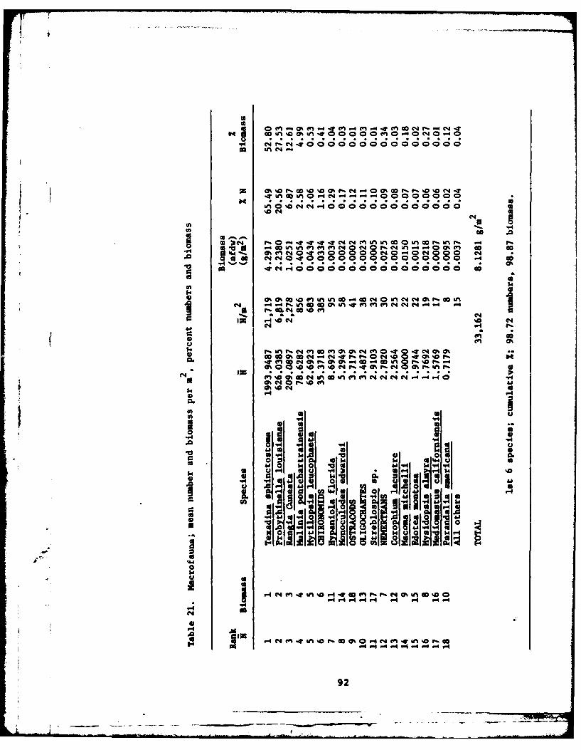
go un C-4.
l 000000
al 00 0
IQ ~C 0 C 0 aC;0 0 o o80 ; 0
0 0
k f- n .t(4 4 Go 0F)00% 0 0C0 000
I4 9= ........... I a! 0!..... W
a% C44 .%%DC00De
0P.
0 of 4
604 .
0 w 0 VW 44 P4 wsq4 -A
I- 4. a.~ 4 6 004 4 UI *c J 4.1
"4Ui~4 I a.o~I"4641-4 101 -
U1 4,-4 A . V
P4C 0 0.4 roCI% 4C. V , a -0P4 P- Id 4 4 J-1-4P*9

control, while biomass was 41%. The mean number of meiofauna animals inall samples from both study sites was 737.2/10cm2 , and biomass was0.8650mg/10cm 2.
Discussion
In order to assess the effects of hydraulic shell dredging on thebenthic fauna of Lake Pontchartrain, the total abundance, relativeabundance, species composition, and community structure at an experimen-tally dredged site and a nearby control site have been examined. Anumber of statistical and numerical methods have been used in an attemptto distinguish the effects of the hydraulic shell dredging on the structureof the benthic community from the effects of other environmental stresses,both natural (such as abrupt salinity fluctuations) and anthropogenic(such as toxic substances).
In addition to its relative importance in food web dynamics inshallow estuarine systems such as Lake Pontchartrain, the benthic com-munity is also more vulnerable to any environmental stresses than anyother group. The sedentary habits of benthic organisms subject them toa greater array of stresses that mobile groups could avoid. This vulner-ability makes the benthos the best indicator of environmental stress inestuarine systems (Copeland and Bechtel 1971). Consequently, manypublished studies of the effects of various stresses on benthic communi-ties exist, with varied evaluations of the results. A common problemwith many of these "before and after" studies is the degree to whichlarge-scale natural fluctuations in the community can mask changes dueto environmental stress (Eagle 1975). The use of a control site, whiledoubling the number of samples needed, is necessary for examining thedegree to which fluctuations are natural or maninduced. In addition,long-term monitoring, such as has been carried out along the coast ofSweden (Ankar and Elmgren 1976; Leppikoski 1975; and Rosenberg andM5ller 1979) is valuable in separating natural from induced fluctuations.Historical- data from Lake Pontchartrain, while interesting, are semi-quantitative at best, so reliance on the use of control site data hasbeen necessary in this study.
One striking feature of the benthic community of Lake Pontchartrain*is its consistently low species diversity. Overall species diversity of
the lake obtained during the initial survey of 86 stations was 1.370.04 (Bahr et al. 1980). The initial and final average measures ofdiversity at the dredged experimental site and the undredged controlsite were no' significantly different from each other, and while slightly
..4 lower than the mean for the lake, were not significantly different fromearlier values from that area.
Values for species diversity have been shown by various investi-gators to have a negative correlation with environmental stress,particularly with pollution (Wilhm and Dorris 1968; Woodwell 1970;Copeland and Bechtel 1971; Goodman 1975; and Ruggiero and Merchant1979).
93
I
Diversity measures are reported using both log and log; Alldiversities quoted in this study have been converteg to log . Thecomonly accepted standards for polluted systems then become: H < 1.443,severe pollution; 1.443 < H < 4.328, moderate pollution; H > 4.328,clean water (Wilhm and Dorris 1968). This is an empirical categoriza-tion based on results of extensive environmental sampling. For instance,in a study of the species diversity and water quality in Galveston Bay,Texas, Copeland and Bechtel (1971) found that areas receiving the greatestamount of toxic effluent exhibited the lowest mean annual diversity.
$ Overall benthic diversity in that highly polluted system was 0.8400.374, not significantly different from Lake Pontchartrain.
Gray (1978) has pointed out that the use of Caswell's neutral modelof diversity (Caswell 1976) can place diversity measures related topollution on a more theoretical basis. Briefly, the neutral modelpredicts the level of diversity if no biological interactions, such aspredation or competition, occur. Hutchinson (1958) on the basis ofniche theory, predicts a higher diversity where interactions are strong.In testing the neutral model predictions of diversity and evenness, thetable of Caswell (1976) was used. The table is abbreviated, however,and a series of curvilinear regressions were constructed using his tablein order to extend the table to cover a greater range.
The diversity predicted for the experimental site by the neutralmodel was 1.115, not significantly different from the diversity of 1.108± 0.146 occurring at the end of the first year. The predicted value forthe control site was 1.070, not significantly different fr'2 the diversityof 1.068 ± 0.035 occurring. This matching of the neutral model ispredicted theoretically for highly polluted, or disturbed systems, wherespecies equilibrium is altered and higher dominance and lower speciesdiversity ensues, or wherever the influence of abiotic factors swamp theinfluence of biological interactions. Evenness at the control site,0.453 ± 0.029, and the experimental site, 0.579 t 0.055, are also notsignificantly different from the theoretical values of 0.464 and 0.516.
Other low salinity, polluted estuaries have similarly low diversi-ties, for instance, the Baltic, 1.05 (Ankar and Elmgren 1976) and 1.3(Rosenberg and Hdller 1979), Hampton Roads Area "mud" stations 1.590.26 (Boesch 1973).
In addition to measures of diversity, which say nothing about thespecies compositon of a sample or a collection of samples, Haedrich(1975) urges that a measure of overlap be included in all environmental
-. impact statements. He describes data from nine estuaries where areas ofr apparent high pollution have low annual diversity, H, and high overlap,
PS (percent similarity). The species overlap, PS, at the dredging andcontrol sites was 92.86%, indicating the apparent affects of pollutionor disturbance on both sites.
Other measures of comunity structure, such as abundance, showmarked differences at the control and experimental sites. The lack ofrecovery by the end of the first year is evidenced by the reduced abun-dance at the experimentally dredged site. Both meiofauna and msacrofaunacomiunities show reduced abundance. The total meiofauna is reduced to
94
f -
57% at the experimental site compared to the control site. The dominantgroup, the nematodes, are reduced to 38% of the control by this time and42% of mean annual abundance of the control. This pattern of similardiversity measures and different annual abundance continued through thesecond year.
In addition to examining the usual measures of community structuresuch as abundance, species diversity, and overlap at the two sites, acomparison of the distributional pattern of individuals within speciesat each site was made. Species-abundance data from a large enoughsample from a heterogeneous population can usually be fitted to a log-normal distribution (Gray 1979, May 1975). Practical limits to the sizeof samples and the probability of misidentifying a specimen from a rarespecies as a member of a commoner species results more often in thedistribution's being truncated on the left side (Slocumb et al. 1977;Krebs 1972). The method of plotting species-abundance data into geo-metric classes is extremely robust in that any errors arising fromlimited samples, or overly cautious identification, results only in thefirst point in a series (Figure 50) being below the line (Gray and Mirza1979). After plotting data from a series of benthic surveys, Gray andMirza have demonstrated the use of log-normal plots as an indicator ofpollution-induced disturbance on estuarine benthic communities (1979).They postulate that a slope of over 500 would indicate an unpolluted orundisturbed community, whereas a slope of under 350 would indicate acommunity affected by pollution. Plotting the species-abundance datafor the August 1979 collections at the dredging control site and thedredging experimental site (Figure 50) shows an angle of 19°, whichwould indicate a community that has reached an equilibrium under pollutedor disturbed conditions, since transitional communities very often showa break in the line (Gray and Mirza 1979).
Information on mean abundance and mean biomass of several otherbenthic communities has been summarized in Table 22. The average orga-nism in other benthic communities is 32 times larger than the averagefor Lake Pontchartrain macrofauna. Not only are the species which occurin the lake smaller representatives of their genera or families, but thesize of the individuals are smaller than the average for collections ofsome of the same species from other areas in Louisiana and from otherstates. This condition has been noted by taxonomic experts who haveconfirmed species identifications for us.
In addition to small species and to small sizes within species,there were an unusually low total number of species present. In contrastto the mean of 12.01 ± 0.36 species present in the present study collec-tions, Boesch (1973) found 23.00 ± 3.73 in a similar low diversityhabitat. Conner and Simon (1979), in a study on the effects of shelldredging on a soft-bottom community in Tampa Bay, Florida, identified amean of 79.5 benthic species before dredging and 47.5 after dredging.Even with a loss of 41% of the species, Tampa Bay still retained fourtimes as many species as the two study sites in Lake Pontchartrain have.
Darnell, during the course of a survey of benthic invertebrates inLake Pontchartrain in 1953-55 (unpublished manuscript), found the samelimited number of benthic species. He did, however, find a somewhat
95
_ _ _ __
- r - -o .

0
aau
00 0
*0
r4.00
Crj
'0 41 V%.
v-4 096 *ii (.
*00
th
96i-

Table 22. Macrofauna, numbers and biomass from the literature
Sieve -/ m2 Biomass BiomassStudy site size, mm g/m2 mg/animal
Long Island Sound (N. Y.) 1.0 16,466 54.627 3.32(Sanders 1956)
Martha's Vineyard (Mass.) 1.0 2,477 10.362 4.18(Wigley and McIntyre 1964)
Goose Creek (N. Y.) 1.4 1,201 29.460 24.53(Kaplan et al. 1974)
Lynher Estuary (V. K.) 0.5 1,436 13.240 9.22(Warwick and Price 1975)
Baltic (Sweden) 1.0 3,547 10.480 2.95(Ankar and Elmgren 1976)
Tampa Bay (Florida 0.5 18,550 27.505 1.48(Conner and Simons 1979)
Lake Pontchartrain 0.5 33,618 8.128 0.24(This study)
97

different distribution of organisms within the species. His reportednumbers of small gastropods were an order of magnitude lower than foundin the present study. Additionally, Rangia greater than 20 m werefound, as mentioned earlier in this report (p. 23), in numbers farexceeding those found during this study. If biomass determinations hadbeen done on Darnell's collections, his total average biomass wouldprobably have been similar to that found in this study. The differencewould have been in the proportion of biomass found in each species.Rangia would have probably been ranked higher in percent biomass thaneither of the gastropods. Since Rangia are a preferred food of the bluecrab (Callinectes sapidus), with 64% of the crabs' total stomach volumemade up of Rangia (Darnell 1958), it is probable that the documenteddecrease in number of larger (> 20 mm) Rangia has had a significanteffect on food available to blue crabs.
These very high numbers of small organisms are a result of a typicalecological strategy in ecosystems where predation is a major, unpredictablesource of mortality for all life history stages of all species. We canthink of the dredge as a very large, non-selective benthic predator,periodically removing every organism from an area of mud. In addition,a large percentage of the pelagic larvae present in the area are "consumed"by or pumped through the dredge, which pumps 83.23 m3/min while activelydredging. There is, then, an advantage to be gained by any species thatmatures rapidly and reproduces frequently. This is typical "r-strategy,"and usually is found in small organisms with rapid population growth(Miller 1979, Southwood 1977).
Many small organisms would fit this description, thus the highdominance by the two small hydrobiid gastropods requires additionalexamination of ecological factors. The altered bulk densities of thesediments would affect species equally. Any small species remaining inthe area after the 20 years of dredging that occurred before 1953 wouldprobably have had a somewhat more evenly distributed abundance if dredgingwere the only factor. It is probable that increasing levels of pollutionin the last 20 years have also had an effect. In order to ensure thatdifferent levels of pollution at the two study sites did not mask orconfuse the effects of dredging in the study by causing a differentialmortality due to pollution stress, several sets of sediment samples wereanalyzed for PCB content. The two study sites had sediment levels thatwere not significantly different (P S 0.05) from each other. The meanof 0.32 ± 0.04 pg/g PCB's found at the two study sites during the firstmonths of the study is significantly higher than levels of 0.17 ± 0.13 pg/gquoted for levels in the Great Lakes (Eisenreich, Hollod, and Johnson1979). Amphipods are, as a group, more sensitive to toxic substancesthan molluscs or polychaetes (Reish and Barnard 1979). Polychaetes varyin sensitivity. Species known to be tolerant to many toxic substances,which, in fact, are used as indicators of polluted conditions, includeCapitella capitata, Nereis succinea, Streblospio benedicti, and Polydoraligni (Reish 1979). Molluscs seem somewhat less sensitive to certaintoxic substances (Menzel 1979). Hydrobiid gastropods are particularlytolerant of chlorinated hydrocarbons (Brown 1980). Differential responseto the increasing levels of toxic substances would appear to be animportant factor in the high dominance of the two hydrobiid gastropods,Probythinella louisianae and Texadina sphinctostoma.
98

1T
Suimmary
We have examined the effects of hydraulic clam shell dredging onthe benthic fauna of Lake Pontchartrain. We have found that it islikely that species numbers were reduced by dredging that occurredbefore 1954 as shown by the low species number in Darnell's unpublishedwork. Further changes in benthic community structure, such as lowered
diversity and lowered evenness caused by the increased dominance of twospecies, may be attributed to increasing levels of toxic substances inthe sediments. Present day dredging in this low diversity benthiccommunity has significant effects on the abundance of both macrofaunaand meiofauna through the first year after the experimental dredging atthe study site and significant effects through the second year on themacrofauna. We cannot yet say whether the area has recovered to theoriginal, initial abundance.
(
99

OVERVIEW
Lake Pontchartrain is a large, shallow, semi-enclosed estuarinesystem that has sustained a clam dredging industry since 1933. Tounderstand the effects of shell dredging in this system, it is necessaryto understand the difference between the nature of clam shell dredgingand oyster shell dredging. In the latter, disturbances are concentratedover reef deposits and, although they may be severe, they are somewhatlocalized, resulting in a "pothole" effect. Large areas of a system maybe left unaffected by this type of shell dredging. In clam shell dredging,dredges move continuously, extracting Rangia shells, which are dispersedwidely over most of the system. Presently in Lake Pontchartrain, 44 ofthe lake is open to dredging, and it has been shown that an area equivalentto this is dredged in from 1.4 to 2.3 years. Considering the 48-yearspan of shell dredging in Lake Pontchartrain, the inevitable conclusionis that the system as a whole is affected by shell dredging. Estimatingthe extent is contingent on demonstrating the magnitude of shell dredgingeffects. The present study has quantified physical effects to thesediments chemical effects to the sediments, and water column, andbiological effects to the benthic invertebrate community.
The immediate physical effects of shell dredging on the watercolumn were found to be temporary, with most of the spoil sinking rapidlythrough the water column and spreading out on the bottom, filling intrenches or cuts. Very little material contributes to the visibleplume, which is of a temporary nature and has little relationship to thedistribution of dredged sediments. The effects to the redepositeddredged sediments are more substantial and take the form of reduced bulkdensities. Bulk densities of fresh dredge spoil were found to be1.22 g/cm3 . Bulk densities below 1.30 g/cm3 are considered fluid mud byDiaz and Boesch (1977), who conclude that "its unique physical propertieshave deleterious effects on benthic fauna." Bulk densities of less than1.30 g/cm3 have been found at stations in Lake Pontchartrain, includingin an area that has been closed to dredging for 27 years. In a laboratoryconsolidation experiment, dredge spoil was found to consolidate 39% of a75 cm high sediment column in seven months. Under field conditions inthe shallow lake, consolidation provides the mechanism for maintaininglow bulk densities as wave-resuspended sediments fill in depressions.Low sediment bulk densities can be detrimental to sedentary benthicorganisms, particularly on larger and denser organisms, which wouldcontinually sink in the sediments.
Resuspension of sediments by wind-induced wave action was found tooccur to a greater degree at the dredged site than at the control site.This was evidenced by greater increases in the water column at the
- dredged site of particulate iron and maganese on day 20, following threedays of high winds.
The effects of shell dredging on the nutrients nitrogen and phos-phorous and on the heavy metals iron, manganese, lead, zinc, and copperwere investigated in the water column, in the sediment-water interface,and in the sediments. All parameters studied were affected by dredgingin all three environments. Many of these effects, however, were of rel-atively short duration, lasting from a matter of hours to one to two
100
-A -- - - - -
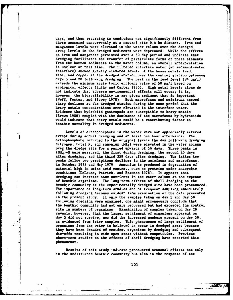
days, and then returning to conditions not significantly different fromthose measured concurrently at a control site 0.4 km distant. Iron andmanganese levels were elevated in the water column over the dredgedarea; levels in the dredged sediments were depressed. While the effectson iron and manganese persisted over a 50-day period and indicate thatdredging facilitates the transfer of particulate forms of these elementsfrom the bottom sediments to the water column, an overall interpretationis unclear at this time. The filtered interface water (at sediment-waterinterface) showed greatly elevated levels of the heavy metals lead,zinc, and copper at the dredged station over the control station betweeendays 5 and 20 following dredging. The peak in the lead level (84 Vg/l)exceeds the minimum acute toxic effluent value of 50 pg/1 based onecological effects (Luthy and Carter 1980). High metal levels alone donot indicate that adverse environmental effects will occur; it is,however, the bioavailability in any given sediment that is important(Neff, Foster, and Slowey 1978). Both macrofauna and meiofauna showedsharp declines at the dredged station during the same period that theheavy metals concentrations were elevated in the interface water.Evidence that hydrobiid gastropods are susceptible to heavy metals(Brown 1980) coupled with the dominance of the macrofauna by hydrobiidswould indicate that heavy metals could be a contributing factor tobenthic mortality in dredged sediments.
Levels of orthophosphate in the water were not appreciably alteredexcept during actual dredging and at least one hour afterwards. Theorthophosphate returned to the original levels the day following dredging.Nitrogen, total N, and ammonium (NH4) were elevated in the water columnoveT the dredge site for a period upwards of 50 days. Three peaks in(NH4)-N were measured, the first during dredging, the second 20 daysafter dredging, and the third 259 days after dredging. The latter twopeaks follow two precipitous declines in the meiofauna and macrofauna,in October 1978 and May 1979. Ammonium is produced in degradation ofmaterial high in amino acid oontent, such as proteins under anaerobicconditions (DeLaune, Patrick, and Brannon 1976). It appears thatdredging can increase some nutrients in the water column at the expenseof benthic organisms. The long-term effects of shell dredging on thebenthic community at the experimentally dredged site have been pronounced.The importance of long-term studies and of frequent sampling immediatelyfollowing dredging becomes evident from examination of the data presentedin the present study. If only the samples taken on day 5 and day 50following dredging were examined, one might erroneously conclude thatthe benthic community had not only recovered but had exceeded the controlsite in numbers of organisms. Examination of samples taken on day 20reveals, however, that the larger settlement of organisms apparent onday 5 did not survive, nor did the increased numbers present on day 50,as evidenced from later samples. This phenomenon of large settlement oforganisms from the water is believed to occur in dredged areas becausethey have been denuded of resident organisms by dredging and subsequentdie-offs resulting in wide open areas without competition. Previousshort-term studies on the effects of shell dredging have recorded thisphenomenon.
Results of this study indicate pronounced seasonal effects not onlyin the undisturbed benthic community but also in the response of the
101
LA. -
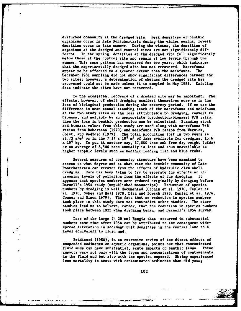
disturbed comunity at the dredged site. Peak densities of benthicorganisms occur in Lake Pontchartrain during the winter months; lowestdensities occur in late summer. During the winter, the densities oforganisms at the dredged and control sites are not significantly dif-ferent. In the spring, densities at the dredged site fall significantlybelow those at the control site and remain at low levels through thesummer. This same pattern has occurred for two years, which indicatesthat the experimentally dredged site has not recovered. Macrofaunaappear to be affected to a greater extent than the seiofauna. TheDecember 1981 sampling did not show significant differences between thetwo sites; however, a determination of whether the dredged site hasrecovered could not be made unless it is sampled in May 1981. Existingdata indicate the sites have not recovered.
To the ecosystem, recovery of a dredged site may be important. Theeffects, however, of shell dredging manifest themselves more so in theloss of biological production during the recovery period. If we use thedifference in mean annual standing stock of the macrofauna and meiofaunaat the two study sites as the loss attributable to dredging, convert tobiomass, and multiply by an appropriate (production/biomass) P/B ratio,then the loss in benthic production can be calculated. Standing stockand biomass values from this study are used along with macrofauna P/Bratios from Robertson (1979) and meiofauna P/B ratios from Warwick,Joint, and Radford (1979). The total production lost in two years is21.73 g/m2 or in the 7.17 x l08 m2 of lake available for dredging, 15.6x 10⁶ kg. To put it another way, 17,000 tons ash free dry weight (afdw)or an average of 8,500 tons annually is lost and thus unavailable tohigher trophic levels such as benthic feeding fish and blue crabs.
Several measures of comunity structure have been examined toassess to what degree and at what rate the benthic comunity of LakePontchartrain can recover from the effects of hydraulic clam shelldredging. Care has been taken to try to separate the effects of in-creasing levels of pollution from the effects of the dredging. Itappears that species numbers were reduced originally by dredging beforeDarnell's 1954 study (unpublished manuscript). Reduction of speciesnumbers by dredging is well documented (Cronin et al. 1970, Taylor etal. 1970, Sykes and Hall 1970, Diaz and Boesch 1973, Kaplan et al. 1974,Conner and Simon 1979). The fact that no reduction in species numberstook place in this study does not contradict other studies. The otherstudies lead us to believe, rather, that the reduction in species numberstook place between 1933 when dredging began, and Darnell's 1954 survey.
Loss of the large (> 20 um) Rangia that occurred in substantialnumbers some time after 1954 can be attributed to the consequent wide-
- spread alteration in sediment bulk densities in the central lake to alevel equivalent to fluid mud.
Peddicord (1980), in an extensive review of the direct effects ofsuspended sediments on aquatic organisms, points out that contaminatedfluid muds can have substantial, acute impacts on benthic fauna. Theseimpacts vary not only with the types and concentrations of contaminantsin the fluid mud but also with the species exposed. Shrimp experiencedless mortality in tests with contaminated sediments than did young
102

crabs, which died during molting (Peddicord et al. 1975). In additionto direct effects on adult macrofauna, fluid muds can create indirecteffects where they form a blanket over bottom areas critical to thejuvenile life stages of aquatic organisms (Hirsch et al. 1978).
An additional effect of the destabilization of contaminated sedi-ments is an increase in the availability of the toxic substances boundto microparticulates to filter feeders or to other organisms in thewater column. Recently, Harding and Phillips (1978) found that diatomscan absorb (or adsorb) low concentrations of PCB's bound to particles,which effectively reduces photosynthetic activity. It has been assumedthat PCB's were extracted from the sediment by benthic organisms andreintroduced to the food chain in the overlying water column (Eisenreichet al. 1980), since PCB's are not very soluble, and once introduced intothe water, are rapidly sedimented. Introduction of PCB's into theplanktonic food web by resuspension of contaminated sediments is one ofthe mechanisms by which fish in the Great Lakes have reached FDA action-able levels while the water concentrations remain below detection levels(Eisenreich et al. 1979).
Species diversity in a brackish system is never as high as in afreshwater or marine system. It is probable, however, that in the pastLake Pontchartrain would have had a species diversity of 2.4 to 2.8,similar to other healthy brackish systems (Rosenberg and Idller 1979).It is difficult to separate the effects of dredging from the effects ofpollution on species diversity. For example, small gastropods have agreater tolerance for certain toxic substances than other small organismssuch as amphipods and polychaetes (Menzel 1979, Reisch and Barnard
*1979). They are thus able to use the resources made available by theloss of the larger Rantia (attributable to sediment destabilization) andthe decreased competition from more sensitive organisms.
In addition to the lowering of species numbers, any concomitantlowering of species diversity by dredging had probably begun beforeDarnell's study. Diversity has been further lowered by pollution to thepoint where the only species remaining are opportunistic, or "weed,"species. These species are small; individuals within the species aresmall, and appear to breed frequently, with large fluctuations in popu-lation densities. An examination of the meiofauna in the data appendix(Appendix Bl) will show no sampling period when small, juvenile gastropodsdid not appear in the samples. Occasionally, numbers of meiofauna-sizegastropods would equal the number of gastropods in the macrofauna on anequal area basis. This typical pattern of "r-selected" species assem-blages is caused by the dredging in the sense that dredging is acting asa "non-selective" predator, and only those species that breed morefrequently than an average of than once every 1.4 to 2.3 years willremain in the system.
We have discussed the adaptations within the macrofaunal componentsof the benthic community. The meiofaunal components show the sameadaptations. If we consider copepods as representative of the meiofaunalgroups present, we find the number of species present very low (Fleeger,Appendix D). Species diversity (H') of the meiobenthic copepods at theexperimental site was not significantly different (P S 0.05) from the
103

IT
species diversity at the control site, nor from the initial speciesdiversity of the macrofauna. At the end of the first year of the study,August 1979, the measured diversity at the experimental site continuedto not be significantly different from the control site and the macrofaunaspecies diversity at the two study sites. This was also true in August1980.
In summary, Lake Pontchartrain is a perturbed system, the result,historically, of continuous perturbation from shell dredging operationsand from pollution. Shell dredging produces fluid mud that is deleteriousto benthic fauna. Contaminated fluid mud is potentially even moreharmful to benthic organisms. To what extent this potential is actuallyrealized in a particular system will depend on the occurrence and arealdistribution of the fluid mud (Peddicord 1980). In Lake Pontchartrain,shell dredging has spread fluid mud over nearly all of the open lake.
Sediments at the dredged and control sites in central Lake Pontchar-train were found to contain high levels (0.32 pg/g) of PCB's. Fluidmuds have the potential for producing high suspended sediment concentra-tions (Peddicord 1980), and wave action in Lake Pontchartrain has thepotential for resuspending sediments frequently (Swenson 1980). Transferof PCB's from microparticulates to marine phytoplankton has been demon-strated as has the fact that PCB's inhibit phytoplankton photosynthesisand cell division (Harding and Phillips 1978) and thus, ultimately,primary production. Reduced primary production means less food eventuallyreaches the bottom. The combined effects of contaminated fluid mud onthe bottom and reduced food availability to benthic organisms haveresulted in a benthic community in the open lake that is characterizedby: (1) a low number of species; (2) a low species diversity; (3) smallindividuals; and (4) a low biomass. These conditions have developedover many years, and it is not possible to predict, even if shell dredgingoperations were to cease, whether, or to what extent, the lake systemwould recover.
104

CONCLUSIONS
The results of the experimental shell dredging, assessed in thelight of the literature reviewed for this study, lead to the followingconclusions:
(1) Hydraulic shell dredging in Lake Pontchartrain produces fluidmud of a bulk density of 1.22 g/cm3 from silty clay sediments. Low bulkdensity sediments persist for long periods in the lake.
(2) Shell dredging at a site in the central region of the lakeproduced a detrimental effect on the macrofauna and the meiofauna,resulting in lower densities in spring and summer at the dredged sitecompared to the control site. These effects have persisted for twoyears.
(3) Shell dredging resulted in a loss of production by the benthiccommunity during the two years of the study. Biomass production wasreduced by 38% the first year and by 25% the second year after dredging.Over the two-year period, a total of 32% of the biological productionwas lost at the dredged site compared to the control site.
(4) Seasonal patterns of settlement from the water column ofbenthic larvae and juveniles during late fall produce similar abundancesat the two study sites. Differential survival at the two sites resultedin a loss in abundance and in biomass at the dredged site and a gain inthese two parameters at the control site by late spring. Consequently,the dredged site appears not to have fully recovered from the effects ofhydraulic clam shell dredging.
(5) Shell dredging did not produce a change in species diversitybetween the dredged site and the control site. Lake Pontchartrain has alow species diversity compared to other low salinity systems. Diversityhas probably been reduced in the past by pollution and by the dredgingof contaminated sediments. Presently, shell dredging is affecting theabundance of the animals in the benthic community.
(6) The benthic community of Lake Pontchartrain has reached anequilibrium with present levels of pollution and consists of a lownumber of species characterized as being tolerant of pollution.
(7) On a system-wide basis, the production of fluid mud, loweredsediment bulk densities, resuspension of contaminated sediments, andlowered primary production in the water column together have the poten-tial to maintain a benthic community of low biomass in the open lake.Less food is thus available to benthic-feeding organisms such as fishand blue crabs.
105
Mau-"

LITERATURE CITED
American Public Health Assoc. 1975. Standard methods for the examinationof water and wastewater. 14th Ed. APHA-AWWA.
Ankar, S., and R. Elmgren. 1976. The benthic macro- and meiofauna ofAnko-Landsort Area (Northern Baltic proper). Contr. Ask5 Lab.No. 11. 115 pp.
Arndt, R. H. 1976. The shell dredging industry of the Gulf Coastregion. pp. 13-48. In A.Bouma (ed.) Shell dredging and its influ-ence on Gulf Coast environments. Gulf Publishing Co. Houston, Tex.
Austin, E. R., and G. F. Lee. 1973. Nitrogen release from lake sediments.J. Wat. Pollut. Control Fed. 45:870-879.
Bahr, L. M. Jr., J. P. Sikora, and W. B. Sikora. 1980. Macrobenthicsurvey of Lake Pontchartrain, Louisiana, 1978. pp. 659-710. InJ. H. Stone (ed.) Environmental analysis of Lake Pontchartrain,Louisiana, its surrounding wetlands and selected land uses. CEL,CWR, LSU, BR, LA 70807. Prepared for U. S. Army Engineer District,New Orleans. Contract No. DACW 29-77-C-0253.
Barrett. B. 1976. Grain size analysis of bottom sediments in LakesMaurepass and Pontchartrain. pp. 145-154. In An inventory andstudy of the Lake Pontchartrain-Lake Maurepasesturine complex.Louisiana Wildlife and Fisheries Commission, New Orleans, La.Tech. Bull. 19.
Berg, R. H. 1970. The oxygen uptake demand of resuspended bottomsediments. U.S. EPA Water Pollution Control Research Series16070DC09/70. 34 pp.
Bloom, S., S. Santos, and J. Field. 1977. A package of computer programsfor benthic community analyses. Bull. Mar. Sci. 27:577-580.
Boesch, D. 1973. Classification and community structure of macrobenthosin the Hampton Roads area, Virginia. Mar. Biol. 21:226-244.
1977. Application of numerical classification in ecologicalinvestigations of water pollution. Ecol. Res. Ser. EPA-600/3-77-033.
Bortleson, G. C. 1970. The chemical investigation of recent lakesediments from Wisconsin lakes and their interpretation. Ph.D.
1 " Thesis, Univ. of Wisconsin-Madison, 278 pp.
Bremner, J. H. 1965. Total nitrogen. In C. A. Black (ed.), Methods ofSoil Analysis, Part 2. Agronomy 9:1-49-1178. Amer. Soc. Agron.Madison, Wis.
Bricker, 0. P., and B. N. Troup. 1973. Sediment-water exchange inChesapeake Bay. Proc. 2nd Internat. Estuar. Conf. on Recent Advancesin Estuar. Res. Myrtle Beach, South Carolina (mimeo), 42 pp.
106

Brown, L. 1980. The use of Hydrobia jenkinsi to detect intermittenttoxic discharges to a river. Water Res. 14:941-947.
Byrnes, B., D. Keeny, and D. Graetz. 1972. Release of anmonia-N fromsediments to waters. Proc. 15th Conf. Great Lakes Res. 15:249-259.
Caswell, H. 1976. Community structure: A neutral model analysis.Ecol. Monogr. 46:327-354.
Conner W., and J. Simon. 1979. The effects of oyster shell dredging onan estuarine benthic community. Estuar. Coastal Mar. Sci. 9:749-758.
Copeland, B., and T. Bechtel. 1971. Species diversity and water qualityin Galveston Bay, Texas. Wat., Air, Soil Pollut. 1:89-105.
Coull, B., and S. Bell. 1979. Perspectives of marine meiofaunal ecology.pp. 189-216. In R. Livingston (ed.). Ecological processes incoastal and marine environments. Plenum Press, NY.
Cronin, L., R. Biggs, D. Flemer, H. Pfitzenmeyer, F. Goodwyn, W. Dovel,and D. Ritchie. 1970. Gross physical and biological effects ofoverboard spoil disposal in upper Chesapeake Bay. Natural ResourcesInst. Spec. Rep. 3. Univ. of Maryland. 66 pp.
Darnell, R. 1958. Food habits of fishes and larger invertebrates ofLake Pontchartrain, Louisiana, an estuarine community. Publ. Inst.Mar. Sci., Univ. Texas 5:343-416.
_1979. (unpublished manuscript).
DeLaune, R. D. W. H. Patrick Jr., and J. M. Brannon. 1976. Nutrienttransformations in Louisiana salt marsh soils. Louisiana StateUniversity, Center for Wetland Resources, Baton rouge, LA. SeaGrant Publ. No. LSU-SG-72-04.
Diaz, R. and D. Boesch. 1977. Impact of fluid mud dredged material onbenthic communities of the tidal James River, Virginia. Tech. Rep.D-77-45. by Virginia Institute of Marine Science, Division ofBiological Oceanography, Gloucester Point, Va., uader contract tothe U.S. Army Engineer Waterways Experiment Station, CE, Vicksburg,Miss.
Dow, D. D., and R. E. Turner. 1980. Structure and function of the phy-toplankton community in Lake Pontchartrain, Louisiana. In J. H.Stone (ed.). Environmental analysis of Lake Pontchartrain, Louisiana,its surrounding wetlands and selected land uses. CEL, CWR, LSU,BR, LA 70803. Prepared for U.S. Army Engineer District, New Orleans.Contract No. DACW 29-77-C-0253.
Eagle, R. A. 1975. Natural Fluctuations in a soft bottom benthiccommunity. J. mar. biol. Ass. U.K. 55:865-878.
Eisenreich, S., G. Nollod, and T. Johnson. 1979. Accumulation ofpolychlorinated biphenyls (PCB's) in surficial Lake Superior sedi-ents: atmospheric deposition. Environ. Sci. Technol. 13:569-573.
107

Eisenreich, S., G. Hollod, T. Johnson, and J. Evans. 1980. Polychlori-nated biphehyl and other microcontaminant-sediment interactions inLake Superior. pp 67-94. In R. Baker (ed.). Contaminants andsediments, Vol. I, Fate and transport, case studies, modeling, andtoxicity. Ann Arbor Science, Ann Arbor, Mich.
Gael, B. T. 1980. Computations of drift patterns in Lake Pontchartrain,Louisiana. pp. 39-56. In J. H. Stone (ed.). Environmental analysisof Lake Pontchartrain, Louisiana, its surrounding wetlands, andselected land uses. CEL, CWR, LSU, BR, LA 70803. Prepared forU.S. Army Engineer District, New Orleans. Contract No. DACW29-77-C-0253.
Gahler, A. R. 1969. Sediment-water nutrient interchange. Proc. Eutrophi-cation-Biostimulation Assessment Workshop, Univ. of California-Berkeley,243-257.
Goodman, D. 1975. The theory of diversity-stability relationships inecology. Quart. Rev. Biol. 50:237-266.
Gorham, E. and D. J. Swaine. 1965. The influence of oxidizing andreducing conditions upon the distribution of some elements in lakesediments. Limnol. Oceanogr. 10:268-279.
Gotoh, S. and W. H. Patrick Jr. 1972. Transformation of manganese in awaterlogged soil as affected by redox potential and pH. Soil Sci.Soc. Amer. Proc. 36:738-742.
Gray, J. S. 1978. The structure of meiofauna communities. Sarsia64:265-272.
1979. Pollution-induced changes in populations. Phil. Trans.R. Soc. Lond. B. 286:545-561.
and F. Mirza. 1979. A possible method for the detection ofpollution-induced disturbance on marine benthic communities. Mar.Poll. Bull. 19:142-146.
Gulf South Research Institute (GSRI). 1972. Surface circulation ofLake Pontchartrain: a wind dominated system. Final Report GSRIProject NS-255. 122 pp.
- Gulf South Research Institute (GSRI). 1974. Environmental impact of" shell dredging in Lake Pontchartrain. Report GSRI Project No.
414-665-41. 275 pp.
Haedrich, R. 1975. Diversity and overlap as measures of environmentalquality. Water Research 9:945-952.
Harding, L., and J. Phillips. 1978. Polychlorinated biphenyls: transferfrom microparticulates to marine phytoplankton and the effects onphotosynthesis. Science 202:1189-1192.
108
Harper, D. E., and S. H. Hopkins. 1976. The effects of oyster shelldredging on macrobenthic and nektonic organisms in San Antonio Bay.pp. 232-279. In A. Bouma (ed.). Shell dredging and its influenceon Gulf Coast environments. Gulf Coast Publishing Co. Houston, TX.
Heard, R. W. 1979. Notes on the genus Probythinella Thiele, 1928(Gastropoda: Hydrobiidae) in the coastal waters of the northernGulf of Mexico and the taxonomic status of Vioscalba louisianaeMorrison, 1965. Gulf Res. Rpts. 6(3):309-312.
Hirsch, N., L. DiSalvo, and R. Peddicord. 1978. Effects of dredgingand disposal or aquatic organisms. Tech. Rep. DS-78-5, by NavalBiosciences Laboratory, Naval Supply Center, Oakland, Calif., undercontract of the U.S. Army Engineer Waterways Experient Station, CE,Vicksburg, Miss.
Ho, C. L., and S. Schneider. 1974. Water and sediment chemistry. InEnviron. Asses. of a La. Offshore Oil Port, Vol. II, Sec. II. LOOP,Inc., New Orleans, LA.
Hopkins, S. H., and L. D. McKinney. 1976. A review of the literaturepertaining to the effects of dredging on oyster reefs and theirassociated faunas. pp. 3-12. In A. Bouna (ed.). Shell dredgingand its influence on Gulf Coast environments. Gulf Coast PublishingCo. Houston, TX.
Hutchinson, G. E. 1958. Concluding remarks. Cold Spring Harbor Symp.Quant. Biol. 22:415-427.
Hynes, H. B. N., and B. J. Greib. 1970. Movement of phosphate andother ions from and through lake muds. J. Fish. Res. Bd. Can.27:653-668.
Jonasson, A., and E. Olausson. 1966. New devices for sediment sampling.Mar. Geol. 4:365-372.
Kaplan, E., J. Welker, and M. Kraus. 1974. Some effects of dredging onpopulations of macrobenthic organisms. Fish. Bull. 72:445-480.
Kemp, G. P. 1978. Personal communication. Coastal Studies Institute,Louisiana State University, Baton Rouge, La.
Krebs, C. 1972. Ecology: The experimental analysis of distribution.Harper and Row, New York. 694 pp.
r Lee, G. F. 1979. Factors affecting the transfer of materials betweenwater and sediments. Water res. center, Univ. of Wisconsin-Madison,Occasional Paper No. 1, 50 pp.
• 1975. Significance of chemical contaminants in dredgedsediments on estuarine water quality. Proc. Estuar. Pollut. Work-shop, Pensacola, Florida.
109

Leppikoski, E. 1975. Assessment of degree of pollution on the basis ofmacrozoobenthos in marine and brackish water environments. ActaAcademiae Aboensis, Ser. B 35:1-90.
Livingstone, D. A., and J. C. Boykin. 1962. Vertical distribution ofphosphorus in Linsley Pond mud. Limnol. Oceanogr. 7:57-62.
Louisiana Wild Life and Fisheries Commission. 1968. The history andregulation of the shell dredging industry in Louisiana. Compiledfor the governor State of Louisiana. 32 pp.
Luthy, R. C., and H. J. Carter. 1980. Leaching characteristics of coalgasification process ash and char. pp 137-167. In R. A. Baker(ed.). Contaminents and sediments. Vol. 2 analysis, chemistry,Biology. Ann Arbor Science, Ann Arbor, Mich.
Maurer, D., W. Leathem, P. Kinner, and J. Tinsman. 1979. Seasonalfluctuations in coastal benthic invertebrate assemblages. Estuar.Coastal Mar. Sci. 8:181-193.
Hay, E. B. 1973. Environmental effects of hydraulic dredging in estuaries.Alabama Mar. Resource Bull. 9:1-85.
Hay, R. 1975. Patterns of species abundance and diversity. pp 81-120.In M. Cody and J. Diamond (eds.). Ecology and evolution of communi-ties. Belknap Press, Cambridge, Mass.
Menzel, W. 1979. Clams and snails [Mollusca: Pelecypoda (exceptoysters) and Gastropoda] pp. 371-396. In C. Hart, and S. Fuller(eds.). Pollution ecology of estuarine-invertebrates. AcademicPress, NY.
Miller, P. 1979. Adaptiveness and implications of small size in teleosts.Symp. zool. Soc. Lond. 44:263-306.
Mortimer, C. H. 1941. The exchange of dissolved substances between mudand water in lakes-Parts I and II. J. Ecol. 29:280-329.
1942. The exchange of dissolved substance between mud andwater in lakes-Parts III and IV. J. Ecol. 30:147-201.
. 1971. Chemical exchanges between sediments and water in theGreat Lakes-Speculations on probable regulatory mechanisms. Limnol.Oceanogr. 16:387-404.
Neff, J., R. Foster, and J. Slowey. 1978. Availability of sediment-i-' absorbed heavy metals to benthos with particular emphasis or
deposit-feeding infauna. Tech. Rep. D-78-42, by Texas A&M ResearchFoundation, College Station, Tex., under contract to the U.S. ArmyEngineer Waterways Experiment Station, CE, Vicksburg, Miss.
Olsen, S. 1964. Phosphate equilibrium between reduced sediments andwater; laboratory experiments with radioactive phosphorus. Verb.int. Verein Theor. Angew. Limnol. 15:333-341.
110

Outlaw, D. C. 1979. Lake Pontchartrain hurricane barrier study:Prototype data acquisition and analysis. Tech. Rep. U.S. ArmyEngineer Waterways Experiment Station, Vicksburg, Miss. (in press).
Patrick, W. H. Jr., R. Gambrell and R. Khalid. 1977. Physicochemicalfactors regulating solubility and bioavailability of toxic heavymetals in contaminated dredged sediments. J. Environ. Sci. Health.A12(9): 475-492.
Peddicord, R. 1980. Direct effects of suspended sediments on aquaticorganisms. pp. 501-536. In R. A. Baker (ed.). Contaminants andsediments, Vol. 1, Fate and transport, case studies, modeling, andtoxicity. Ann Arbor Science, Ann Arbor.
Peddicord, R., V. McFarland, D. Belfiori, and T. Byrd. 1975. Effectsof suspended solids on San Francisco Bay Organisms. Dredge disposalstudy, San Francisco Bay and estuary, Appendix G: Physical impactstudy. U.S. Army Engineer District, San Francisco, Calif.
Perkin Elmer. 1976. Analytical methods for A. A. Spectrophotometry.Perkin Elmer Handbook.
Porcella, D., J. Kumagi, and E. Middlebrooks. 1970. Biological effectsof sediment-water nutrient interchange. J. Sanit. Eng. Div. Am.Soc. Civ. Engrs. 96:911-926.
Reish, D. 1979. Bristle worms (Annelida: Polychaeta) pp. 77-125. InC. Hart, and S. Fuller (eds.). Pollution ecology of estuarineinvertebrates. Academic Press, NY.
, and J. Barnard. 1979. Amphipods (Arthropoda:Crustacea:Amphipoda)pp. 345-370. In C. Hart, and S. Fuller (eds.). Pollution ecologyof estuarine invertebrates. Academic Press, NY.
Richards, A. F., and J. M. Parks. 1976. Marine geotechnology: averagesediment properties, selected literature and review of consolidation,stability, and bioturbation-geotechnical interactions in the benthiclayer. pp. 157-181. In I. N. McCave (ed.). The benthic boundarylayer. Plenum Press, NY.
Robertson, A. 1979. The relationship between annual production:biomass ratios and lifespans for marine macrobenthos. Oecologia38:193-202.
Rosenberg, R., and P. M5ller. 1979. Salinity stratified benthic macro-faunal communities and long-term monitoring along the west coast ofSweden. J. exp. mar. Biol. Ecol. 37:175-203.
Ruggiero, M., and H. Merchant. 1979. Water quality, substrate, anddistribution of macroinvertebrates in the Patuxent River, Maryland.Hydrobiologia 64:183-189.
Ruttner, F. H. 1963. Fundamentals of Limnology. 3rd ed., Univ. ofToronto Press, Toronto. 295 pp.
1l1

II
Sanders, M. 1956. Oceanography of Long Island Sound. 1952-1954. X.Biology of marine bottom comnunities. Bull. Bingham Oceanogr.Coll. 15:345-414.
Sholkivitz, E. R. 1978. The flocculation of dissolved Fe, Mn, Al, Cu.Ni, Co, and Cd during estuarine mixing. Earth and Planetary Sci.Let. 41:77-85.
Slocomb, J., B. Stauffer, and K. Dickson. 1977. On fitting the trun-cated lognormal distribution to species-abundance data using maximumlikelihood estimation. Ecology 58:693-696.
Southwood, T. 1977. Habitat, the templet for ecological strategies?J. Anim. Ecol. 46:337-365.
Sridharan, L. 1973. Aqueous environmental chemistry of phosphorus inlower Green Bay. Ph.D. Thesis, Univ. of Wisconsin, Madison.312 pp.
Strickland, J. D. H., and T. R. Parsons. 1972. A practical handbook ofseawater analysis. Fish. Res. Bd. Can. Bull. 167, Ottawa, Canada.
Swenson, E. M. 1980. General hydrography of Lake Pontchartrain, Louisianapp. 57-155. In J. H. Stone (ed.). Environmental analysis of LakePontchartrain, Louisiana, its surrounding wetlands, and selectedland uses. CEL, CWR, LSU, BR, LA 70803. Prepared for U.S. ArmyEngineer District, New Orleans. Contract No. DACW 29-77-C-0253.
Sykes, J., and J. Hall. 1970. Comparative distribution of molluscs indredged and undredged portions of an estuary with a systematic listof species. Fish. Bull. 68:299-306.
Tarver, J. W., and R. J. Dugas. 1973. A study of the clam Ra ,cuneata, in Lake Pontt.hartrain and Lake Maurepas, Louisiana.Louisiana Wild Life and Fisheries Commission, New Orleans, La.Tech. Bull. 5. pp. 1-97.
Terzaghi, K. 1943. Theoretical soil mechanics. John Uiley and Sons,NY. 510 pp.
Taylor, D. W. 1948. Fundamentals of soil mechanics. John Wiley andSons, NY. 700 pp.
Taylor, J., H. Hall, and C. Saloman. 1970. Molluscs and benthic environ-ments in Hillsborough Bay, Florida. Fish. Bull. 68:191-202.
U. S. Environmental Protection Agency. 1976. Quality criteria forwater. US EPA, Washington, D. C.
Villa, 0., and P. Johnson. 1974. Distribution of metals in BaltimoreHarbor sediments. Annapolis Field Office, Tech. Report 59.
Warwick, R., and R. Price. 1975. Macrofauna production in an estuarinemud-flat. J. mar. biol. Ass. U. K. 55:1-18.
112

Warwick, R., I. Joint, and P. Radford. 1979. Secondary production ofthe benthos in an estuarine environment. pp 429-450. In R. Jeffriesand A. Davy (eds.). Ecological processes in coastal environments.Blackwell Scientific Publication, Oxford.
Wigley, R., and A. McIntyre. 1964. Some quantitative comparisons ofoffshore meiobenthos and macrobenthos south of Martha's Vineyard.Limnol. Oceanogr. 9:485-493.
Wilbm, J., and T. Dorris. 1968. Biological parameters for water qualitycriteria. Bioscience 17:477-481.
Windom, H. L. 1973. Water quality aspects of dredging and dredge spoildisposal in estuarine evnironments (mimeo). Skidaway Inst. Oceanogr.,Savannah, Ga. 19 pp.
Woodwell, G. 1970. Effects of pollution on the structure and physiologyof ecosystems. Science 168:429-433.
Zicker, E., K. Berger, and A. Hasler. 1956. Phosphate release from BogLake muds. Limnol. Oceanogr. 1:296-303.
1
113

-t7-
APPENDIX ABENTHIC MACROFAUNA; LAKE PONTCHARTRAIN CONTROLAND EXPERIMENTAL DREDGING EFFECTS STATIONS
Phylum PlatyhelminthesClass Turbellaria
Phylum Rhynocoela1 unidentified species
Phylum AnnelidaClass OligochaetaClass Polychaeta
H-ypaniola florida HartmanLaeonereis culveri (Webster)Nereis succinea (Frey and Leukart)Parandalia americana (Hartman)Mediomastus caiorniensis HartmanStreblospio .. cf. benedicti WebsterCpitella capitata (Fabricius)Poldora s.
Phylum MolluscaClass Gastropoda.
Probythinella louisianae (Morrison) *Texadina sphinctostoma (Abbott and Ladd)
Class BivalviaMytilopsis leucophaeta (Conrad)Macoma mitchelli DaliMulinia pontchartrainensis Morrison
Phylum AthropodaClass CrustaceaSubclass ostracodaSubclass MalacostracaOrder Isopoda
Cassidinidea lunifrons (Richardson)Edotea montosa (Stimpson)Cyathura polita CStimpson)
order AmphipodaCerapus benthophilus Thomas and HeardCorophium lacustre VanhoffenGrandidier-el labonnieroides StephensonMelita nitida SmithMonoculodes edwardsi Holmes
Order Mysidacea-~ Orderdopsi almyra Bowman
Callinectes sapijdus RathbunRhithropanopeus harisii (Gould)
Class InsectaOrder DipteraFamily ChironomidaeAblabesmyia sp.
In this report P. louisianae P. protera. See Heard (1979) for completetaxonomic discussion.
114
. .. -...... ..

IfIAPPENDIX BTable BIMeiofauna
Experimental Station
Meiofauna (N/lOcm 2 SE) Initial Day 1 Day 2
NEMATODES 228.7 t 20.9 104.9 ± 49.4 167.6 t 41.8
COPEPODS 68.8 t 10.9 33.6 ± 6.7 19.4 ± 4.6COPEPOD NAUPLII 50.4 ± 11.2 44.3 ± 4.1 51.4 t 13.4
OSTRACODS 30.1 ± 6.1 4.6 ± 1.5 2.0 ± 1.4
ROTIFERS 27.0 ± 6.2 27.0 ± 7.0 68.3 ± 21.7
TURBELLARIANS 8.2 ± 1.4 1.0 ± 0.6 8.2 ± 3.7
POLYCHAETES 13.3 ± 3.8 3.1 ± 1.8 2.0 ± 0.8
OLIGOCHAETES 0.5 ± 0.5 0.5 ± 0.5
BIVALVES 37.7 ± 3.2 21.4 ± 6.3 87.1 ± 11.8
GASTROPODS 73.3 ± 8.7 17.8 ± 2.1 32.1 + 12.3
OTHERS 1.5 ± 1.0 0.5 ± 0.5
TOTAL 540.4 ± 10.9 263.3 ± 47.1 439.0 t 81.8
Control StationMeiofauna (-/0cm2 - SE)
Initial
NEMATODES 288.8 ± 21.4COPEPODS 94.2 ± 7.0
COPEPOD NAUPLII 66.7 ± 12.0
OSTRACODS 49.4 ± 4.7
ROTIFERS 13.3 ± 1.3
TURBELLARIANS 9.2 ± 1.3
POLYCHAETES 15.8 ± 5.1
OLIGOCHAETES 1.5 ± 1.0
BIVALVES 68.8 ± 10.1
GASTROPODS 50.9 ± 6.9
OTHERS 3.6 ± 0.5
TOTAL 662.6 ± 43.4
115

Table Bl. (Continued)
Experimental Station
Melofauna (N/lOcm 2 SE) Day 5 Day 20 Day 50
NEMATODES 151.3 ± 12.9 47.4 ± 12.9 234.3 ± 20.3
COPEPODS 13.2 ± 3.6 26.5 ± 8.6 37.2 ± 5.5COPEPOD NAUPLII 58.0 ± 12.7 33.1 ± 9.4 46.9 ± 10.9
OSTRACODS 3.6 ± 1.6 6.1 ± 4.2 31.1 ± 2.3
ROTIFERS 11.7 ± 3.9 13.2 ± 5.0 33.6 ± 8.5
TURBELLARIANS 11.2 ± 2.9 2.0 ± 0.8 15.8 ± 7.4
POLYCHAETES 6.1 ± 1.9 5.6 ± 1.9 22.9 ± 4.0
OLIGOCHAETES 1.0 ± 0.6 0.5 ± 0.5
BIVALVES 33.6 ± 6.3 14.3 ± 4.3 56.5 ± 9.0
GASTROPODS 35.1 5.7 4.1 ± 2.2 67.8 ± 29.1
OTHERS 1.0 ± 0.6 0.5 ± 0.5 1.S t 1.0
TOTAL 329.5 ± 30.0 152.8 ± 42.4 548.0 ± 38.5
Control StationMeiofauna (N/10cm 2 -+SE)
Day 5 Day 20 Day 50
NEMATODES 196.1 ± 55.2 173.2 ± 31.6 457.4 ± 77.6
COPEPODS 26.5 ± 9.0 34.6 ± 6.6 68.3 ± 6.7
COPEPOD NAUPLII 41.8 ± 13.4 68.3 ± 13.3 71.8 ± 4.2
OSTRACODS 17.3 ± 9.8 16.8 ± 4.3 27.0 ± 11.6
ROTIFERS 13.8 ± 2.8 13.3 ± 4.5 36.2 ± 13.1
TURBELLARIANS 5.6 ± 3.0 4.1 ± 1.5 15.3 ± 6.0
POLYCHAETES 6.9 ± 2.9 5.6 ± 2.1 29.6 ± 8.7
OLIGOCHAETES 1.5 ± 1.0 2.6 ± 1.5
BIVALVES 45.3 ± 12.3 38.2 ± 10.8 36.2 ± 12.1
GASTROPODS 70.8 ± 21.4 44.8 ± 16.3 56.6 ± 31.6
OTHERS 1.5 ± 0.5 4.1 ± 2.8 3.1 ± 2.4
TOTAL 427.8 ± 119.9 405.9 ± 71.2 803.7 ± 161.0
116
,n

Table B1. (Continued)
Experimental Station- 2Meiofauna (N/lOcm + SE) Day 205 Day 235 Aug 79
NEMATODES 264.9 ± 52.8 324.4 ± 60.2 202.7 ± 30.4
COPEPODS 108.0 ± 25.2 40.7 ± 7.3 151.8 ± 21.0COPEPOD NAUPLII 118.2 ± 25.7 32.1 ± 6.2 38.4 ± 1.9
OSTRACODS 18.8 ± 3.1 53.0 ± 9.6 45.1 ± 23.7
ROTIFERS 28.5 ± 7.4 44.8 ± 11.0 31.9 ± 4.3
TURBELLARIANS 43.3 ± 14.0 13.8 ± 1.7 3.1 ± 2.4
POLYCHAETES 12.2 ± 5.0 3.6 ± 1.8
OLIGOCHAETES 0.5 ± 0.5
BIVALVES 7.1 ± 3.9 0.5 ± 0.5 33.5 ± 8.1
GASTROPODS 7.7 ± 5.0 1.0 ± 0.6 47.4 " 8.0
OTHERS 1.5 ± 1.0 2.5 ± 1.0 1.0 ± 0.6
TOTAL 609.6 ± 76.9 517.4 ± 83.4 552.6 + 53.8
Control StationMelofauna (-/l2cm SE)
Day 205 Day 235 Aug 79
NEMATODES 592.6 ± 44.0 712.0 ± 43.7 238.0 ± 94.9
COPEPODS 58.8 ± 13.9 81.5 ± 5.3 56.9 ± 13.0COPEPOD NAUPLII 69.3 ± 15.1 70.8 ± 12.9 58.0 ± 14.6
OSTRACODS 28.5 ± 8.6 88.6 ± 16.6 236.9 ± 52.3
ROTIFERS 8.7 ± 1.5 42.8 ± 17.9 93.3 ± 16.6
TURBELLARIANS 15.3 ± 7.0 79.5 ± 11.9 8.2 ± 0.8
POLYCHAETES 17.8 ± 9.0 6.1 ± 2.8 1.0 ± 1.0
OLIGOCHAETES 0.5 ± 0.5
BIVALVES 2.1 ± 1.2 3.6 ± 1.0 46.0 ± 7.4
p GASTROPODS 13.6 ± 1.6 8.7 ± 1.7 41.8 ± 14.1
OTHERS 1.5 ± 1.0 0.5 ± 0.5 36.2 ± 13.8
TOTAL 720.7 ± 131.5 1094.1 ± 41.3 921.3 ± 85.4
117

Table Bi. (Continued)
Experimental Station
Meiofauna (N/lOcm 2 SE) Aug 80 Dec 80
NEMATODES 529.2 ± 115.9 1242.2 ± 163.9COPEPODS 70.3 ± 19.1 94.2 ± 10.9
COPEPOD NAUPLII 147.7 ± 39.4 25.0 ± 5.1
OSTRACODS 5.1 ± 1.0 22.9 ± 2.9
ROTIFERS 86.1 ± 23.3 87.1 ± 27.4
TURBELLARIANS 8.2 ± 1.4 44.8 ± 7.3
POLYCHAETES 73.4 ± 18.0 84.0 ± 8.6
OLIGOCHAETES 2.5 ± 1.3 7.1 ± 2.1
BIVALVES 16.3 ± 6.8 48.4 ± 9.7
GASTROPODS 101.4 ± 28.5 32.1 ± 10.9
OTHERS 1.5 ± 0.5 5.6 ± 1.0
TOTAL 1041.5 ± 173.4 1693.4 ± 197.1
Control Station
Meiofauna (K/l0cm 2 ± SE)Aug 80 Dec 80
NEMATODES 377.4 ± 20.9 1278.3 ± 163.1
COPEPODS 58.1 ± 6.5 60.6 ± 8.5
COPEPOD NAUPLII 170.1 ± 21.3 32.1 ± 2.5
OSTRACODS 4.1 ± 2.0 24.4 ± 4.3
ROTIFERS 28.6 ± 7.6 85.1 ± 4.6
TURBELLARIANS 4.6 ± 1.8 38.2 ± 17.8
POLYCHAETES 65.2 ± 6.4 64.2 ± 5.1
OLIGOCHAETES 23.9 ± 7.1 3.6 ± 1.7
BIVALVES 26.5 ± 12.5 14.8 ± 2.8
GASTROPODS 53.5 ± 12.5 28.5 ± 10.7
OTHERS 3.1 ± 2.0 5.6 ± 3.2
TOTAL 817.0 ± 52.8 1623.1 ± 199.0
118

Table B2Macrofauna
Control StationMacrofauna (N/m2 - SE) Initial Day 5 Day 20
BIVALVES MClams 0- 2 1068 ± 165 596 ± 172 141 ± 27Rangia cuneata 2-10 472 ± 32 490 ± 73 324 ± 51
10-20 4 ± 4 7 ± 420-30
> 30Mulinia pontchartrainensis 2-10 1032 ± 80 1402 ± 226 1071 ± 129Macoma mitchelli 0- 2 4 ± 4 4 ± 4
2-10 7± 7 4± 4
10-20 7± 7 15± 7 11± 6
Mytilopsis leucophaeta 0- 2 1166 3 371 1060 ± 203 635 ± 46
2-10 352 ± 82 706 ± 182 792 ± 23610-20
GASTROPODS --Probythinella louisianae 3643 ± 211 3428 ± 675 2407 ± 17Texadna sphinctostoma 29632 ± 570 37500 ± 8944 30358 ± 44POLYCHAETESHypaniola florida 55 ± 13 123 ± so 40 ± 10Laeonereis culveri 4± 4Nereis succineaParandalia americana 4 ± 4Mediomastus californiensis 18 ± 9 7 ± 4 11 ± 6
Streblospio sp. 18 ± 7 36 ± 22 7 ± 4
Capitella capitataPolydora sp.OLIGOCHAETES 4± 4 14± 9 4 ± 4
TURBELLARIANSNEM4ERTEANS 7± 7 22± 6 14 ± 4
CRUSTACEANSEdotea montosa 22 ± 6 14 ± 7 11 ± 0
Cyathura politaMonoculodes edwardsi 7 ± 7 7 ± 7 29 ± 10
Corophium lacustreGrandidierella bonnieroidesMelita nitidaCerapus sp."Myssi s almra 7± 7 7± 4 7 1 4
Copepods 18 ± 18 4± 4
OstracodsRhithropanopOeus harrisii 4± 4
Callinectes sapidusCHIRONOMIDS 501 ± 50 428 ± 55 552 ± 32
TOTAL 37279 ± 1298 45860 ±10607 36432 1. 375
119

Table B2. (Continued)
Control Station
Macrofauna (N/m2 - SE) Day 50 Day 205 Day 235 (May 79)
BIVALVES suClams 0- 2 308 ± 95 8148 ± 773 7294 ± 470
Rangia cuneata 2-10 479 ± 20 349 ± 76 1129 ± 108
10-20 33 ± 19 5 ± 520-30> 30
Mulinia pontchartrainensis 2-10 537 ± 41 512 ± 98 711 ± 122Macoma mitchelli 0- 2 4 ± 4 60 ± 38 22 ± 12
2-10 11 ± 6 22 ± 11 40 ± 410-20 14 ± 7 5 ± 5 4 ± 4
Mytilopsis leucophaeta 0- 2 316 ± 342-10 988 ± 11510-20 11 ± 11
GASTROPODSProbythinella louisianae 5395 ± 1740 12842 ± 131 14970 ± 1189
Texadina sphinctostoma, 28024 ± 9400 27744 ± 566 25311 ± 1231
Hypaniola florida 236 ± 42 104 ± 49 80 t 36
Laeonereis culveriNereis succineaParandalia americana 5 ± 5 7 ± 7
Mediomastus californiensis 25 ± 10 49 ± 38 40 ± 7
Streblospio sp. 40 ± 4 7 ± 7
Capitella capitataPolydora sp. 4± 4
OLIGOCHAETES 22 ± 7 82 ± 38 58 ± 35
TURBELLARIANSNEMERTEANS 18 ± 4 22 ± 0 29 ± 19
CRUSTACEANSEdotea montosa 11 ± 11 22 ± 22 36 ± 7
Cyathura politaMonoculodes edwardsi 94 ± 25 163 ± 22 109 ± 70
Corophium lacustre 7± 7Grandidierella bonnieroides
Melita nitida 7± 7
- Cerapus sp.- Mysidopsis almyra 18 ± 10 27 ± 36 ± 19
Copepods 7 ± 4 14± 14
OstracodsRhithropanopeus harrisii
Callinectes sapidusCHIRONOMIDS 744 ± 95 316 ± 22 149 ± 28
TOTAL 37348 ± 11698 50477 ± 1558 50063 ± 2555
120

'4
Table B2. (Continued)
Control Station
Macrofauna (1/m 2 ± SE) Aug 79 Nov 79 Feb 80
BIVALVES -nClams 0- 2 207 ± 97 716 ± 252 1569 ± 136Rangia cuneata 2-10 1071 ± 109 493 ± 80 461 ± 31
10-2020-30>30 7± 7
Mulinia pontchartrainensis 2-10 2662 ± 60 232 ± 45 47 ± 7Macoma mitchelli 0- 2
2-1010-20 4± 4
Mytilopsts leuCtephuta 0- 2 36 ± 7 203 ± 116 91 ± 252-10 44± 11 356 ± 95 105 ± 6810-20
GASTROPODSProbythinella louisianae 10446 ± 1148 6884 ± 307 18924 ± 165
Texadina sphnctostoma 25122 ± 2269 16778 ± 7905 19567 ± 887
Hypaniola florida 120 ± 11 312 ± 51Laeonereis culveriNereis succineaParandalia americanaMediomastus californiensisStreblospio sp. 4 ± 4 40 ± 7 98 ± 25Capitella capitataPolydora sp.OLIGOCHAETES 7 ± 7 4 ± 4 15 ± 14TURBELLARIANS 4 ± 4NE1RTEANS 7± 7 7± 4 7± 7CRUSTACEANSEdotea montosa 25 ± 13 22 ± 6 18 ± 13Cyathura polita 4 ± 4Monoculodes edwardsi 7 ± 4 559 ± 221Corophium lacustre 4± 4 7± 7Grandidierella bonnieroidesMelita nitida
Cerapus sp. 4± 4 7± 7Mysidopsis almyra 33 ± 23 14 ± 10 7 ± 4Copepods 29± 4
Ostracods 51± 13
Rhithropanopeus harrisii 7± 4
Callinectes sapidus 4± 4
CHIRONOMZDS 581 ± 84 631 ± 53 628 t 62
TOTAL 40263 ± 3651 27078 ± 3758 41955 ±.1130
121

Table B2. (Continued)
Control Station
Macrofauna -9/m2 t SE) May 80 Aug 80 Dec 80
BIVALVES amClams 0- 2 643 ± 241 7 ± 7 4767 ± 623Rangia cuneata 2-10 247 ± 136 94 ± 51 835 ± 50
10-20 44 ± 44 2S ± 20
20-30 7± 4
> 30Mulinia pontchartrainensis 2-10 142 ± 58 36 ± 4 163 ± 23
Macoma mitchelli 0- 22-10 29 ± 7
10-20 1333 ± 383
yt:leprsis leueophaeta- 0- 2 33 ± 6 1380 ± 402
2-10 76 ± 65 47 ± 10
10-20GASTROPODSProbthinella louisianae 17733 ± 570- 5000 ± 820 4067 ± 600
Texadina sphinctostoma 17192 ± 919 8602 ± 1187 24320 ± 3361
POLYMA ThHypaniola florida 47 ± 26 65 ± 7 2S ± 13
Laeonereis culveriNereis succineaParandalia americana 51 ± 13Hediomastus californiensis 7 ± 7 54 ± 6Streblospio sp. 73 ± Si 18 ± 10
Capitella capitata 7± 4Polydora sp. 4± 4
OLIGOCHAETES 7 ± 4 117 ± 54 145 ± 16
TURBELLARIANS 44 ± 13
NEMERTEANS 4 ± 4 211 ± 32
CRUSTACEANSEdotea montosa 22 ± 11CyatEu ra polita
Monoculodes edwardsi 4± 4
Corophium lacustre 4± 4Grandidierella bonnieroidesMelita nitidaCerapus sp.Mysido.sis almyra 7 ± 4 36 ± 20 11 ± 6Copepods 25 ± 14
Ostracods 683 ± 211Rhithropanopeus harrisii
Callinectes sapidusCHIRONOMIDS 167 ± 18 69 ± 7 240 ± 44
TOTAL 36614 ± 1552 14204 ± 1739 38444 ±. 3975
122
LA-V -

Table B2. (Continued)
Experimental Station
Macrofauna (HIM ± SE) Initial Day 1 Day 2
BIVALVES fluClams 0- 2 1707 ± 123 504 ± 63 131 ± 60
Rangia cuneata 2-10 548 ± 20 918 ± 313 385 ± 14310-20 4 ± 4 7 ± 720-30>30 4± 4 4± 4
Mulinia pontchartrainensis 2-10 1038 ± 100 1536 ± 240 795 ± 231Macoma mitchelli 0- 2
2-10 7± 4 4± 410-20 18 ± 7 4± 4
Hytiopsis leucophaeta 0- 2 1024 ± 73 853 ± 212 116 ± 162-10 447 ± 99 520 ± 208 131 ± 4510-20
GASTROPODSProbzthinella louisianae 3330 ± 227 3969 ± 802 1863 ± 848
Texadina sphnctostoma 33208 ± 531 29254 ± 2371 18753 ± 11990POLYCHAETESHypaniola florida 40 ± 22 4 ± 4Laeonereis culveriNereis succineaParandalia americana 4± 4 4 ± 4Mediomastus californiensis 8 ± 7 7 ± 7 4 ± 4Streblospio sp. 25 ± 16Capitella capitataPolydora sp.OLIGOCHAETES 4± 4 4 ± 4TURBELLARIANS 4 ± 4
NEMERTEANS 14± 4 11 ± 7 14 ± 10CRUSTACEANSEdotea montosa 36 ± 7 11 ± 7 14 ± 10Cyathura politaMonoculodes edwardsi 25 ± 7Corophium lacustreGrandidierella bonnieroidesMelita nitidaCerapus sp.Mysidopsis almyra 4 t 4 4± 4
Copepods 76± 76
OstracodsRhithropanopeus harrisii 4 ± 4
Callinectes sapidus 526 ± 25 232 ± 90 450 ± 81
CHIRONOMIDS
TOTAL 42011 ± 1248 379L ± 4360 22689 ± 13428
123
, -*-'"-*------- ______________________ = . ..... . .

Table B2. (Continued)
Experimental Station(N/r ± SE) Day 5 Day 20 Day 50Macrofauna(/ ±SE
BIVALVES mClams 0- 2 251 ± 107 47 ± 25 3145 ± 1533Rangia cuneata 2-10 432 ± 182 265 ± 199 163 ± 54
10-20 4 ± 4 7 ± 7 4± 420-30> 30 737 ± 114
Mulinia pontchartrainensis 2-10 1202 ± 445 29 ± 15Macoma mitchelli 0- 2
2-10 4± 4 4± 4
10-20 11 ± 11
Mytilopsis leucophagta 0- 2 160 ± 57 22 ± 13 138 ± 62
2-10 141 ± 22 40± 40 552 ± 22610-20
GASTROPODSProbythinella louisianae 4139 ± 987 1155 ± 464 8209 ± 3189Texadina sphinctostoma 46494 ± 14323 9404 ± 2689 25489 ± 9634POLYCHAETES
Hypaniola florida 29 ± 16 7 ± 7 331 ± 144
Laeonereis culveriNereis succinea
Parandalia americana 4± 4Mediomastus californiensis 25 ± 10 7 ± 7 44 ± 23Streblospio sp. 36 ± 36 36 ± 14 211 ± 174Capitella capitata 4± 4Polydora sp. 7± 7OLIGOCHAETES 55 ± 39 7 ± 7 11 ± 7TURBELLARIANS
NEMERTEANS 22 ± 0 14 ± 10 25 ± 4CRUSTACEANSEdotea montosa 14 ± 10 22 ± 17 138 ± 16
Cyathura politaMonoculodes edwardsi 22 ± 13 22 ± 17 44 ± 17Corophium lacustre 4 ± 4 14 ± 14 40 ± 18Grandidierella bonnieroidesMelita nitidaCerapus sp..ysidopsis almyra 22 ± 17 14 ± 10 44 ± 19Copepods 156 ± 156 44 ± 31OstracodsRhithropanopeus harrisii 7 ± 7Callinectes sapidusCHIRONOMIDS 679 ± 107 149 ± 58 516 ± 195
TOTAL 53741 ± 15211 11441 ± 3786 39842 t 15532
124
I . _ ,

I
Table B2. (Continued)
Experimental Station
Macrofauna (N/m ± SE) Day 205 Day 235 Aug 79
BIVALVESClams 0- 2 3351 ± 1953 2796 ± 523 94 t 20Rangia cuneata 2-10 599 t 381 396 ± 47 519 ± 118
10-20 14 ± 10
20-30> 30
Mulinia pontchartrainensis 2-10 3083 ± 1718 1209 ± 164 2404 ± 79Macoma mitchelli 0- 2 73 ± 38
2-10 7 ± 4 131 ± 5810-20 7 ± 4
Mtilopets leucophaeta 0- 2 18 ± 18 18 ± 10
2-10 193 ± 193 14 ± 14 7 ± 7
10-20 76 ± 76
GASTROPODSProbythinella louisianae 4495 ± 1741 5432 ± 2081 4168 ± 252Texadina sphinctostoma 12966 ± 9155 8576 ± 3785 9222 ± 1360POLYCHAETESHypaniola florida 138 ± 51Laeonereis culveriNereis succineaParandalia americana 14 ± 7 4 ± 4Hediomastus californiensis 47 ± 13 7 ± 7Streblospio sp. 18 ± 7Capitella capitataPolydora sp. 14 ± 14OLIGOCHAETES 179 ± 156 7 ± 7 29 ± 14TURBELLARIANS
NEMERTEANS 18 ± 4 29 ± 19 7 ± 4CRUSTACEANSEdotea montosa 22 ± 22 44 ± 44 7 ± 7Cyathura politaMonoculodes edwardsi 112 ± 65 51 ± 19oropThium lacustre 410 ± 138Grandidierel la bonnieroidesMelita nitida 7 ± 7Cerapus sp.Mysidopsis almyra 59 ± 31 7 ± 7 62 ± 32
- Copepods 4 ± 4 36 ± 19OstracodsRhithropanopeus harrisii 4 ± 4Callinectes sapidusCHIRONOMIDS 207 ± 38 127 ± 32 559 ± 195
TOTAL 27125 ± 15365 19113 ± 6923 17105 ± 1296
125
-- I
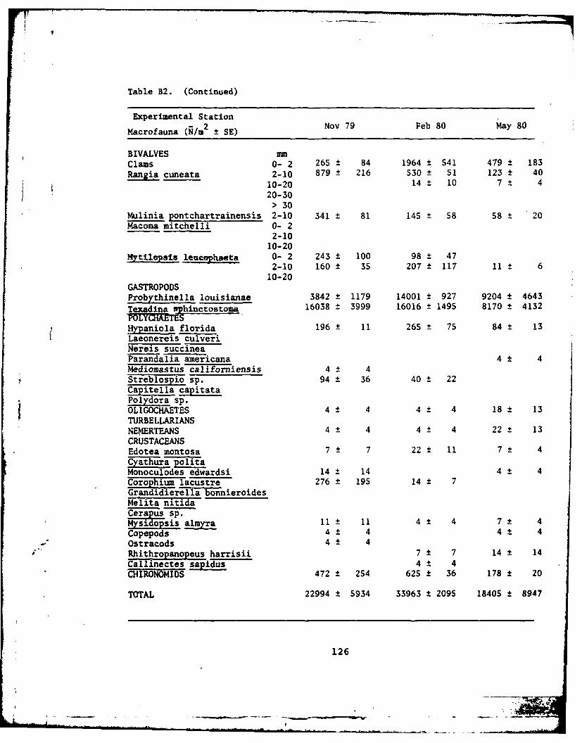
Table B2. (Continued)
Experimental Station
Macrofauna (9/r2 ± SE) Nov 79 Feb 80 May 80
BIVALVES mmClams 0- 2 265 ± 84 1964 ± 541 479 ± 183
Rangia cuneata 2-10 879 ± 216 530 ± 51 123 ± 40
10-20 14 ± 10 7 ± 4
20-30> 30
Mulinia pontchartrainensis 2-10 341 ± 81 145 ± S8 58 ± 20Macoma mitchelli 0- 2
2-1010-20
Mytilopsis leucephasta 0- 2 243 ± 100 98 ± 472-10 160 ± 35 207 ± 117 11 ± 610-20
GASTROPODSProbythinella louisianae 3842 ± 1179 14001 ± 927 9204 ± 4643
ahnctostoma 16038 ± 3999 16016 ± 1495 8170 ± 4132
Hypaniola florida 196 ± 11 265 ± 75 84 ± 13
Laeonereis culveriNereis succineaParandalia americana 4 4Mediomastus californiensis 4 ± 4Streblospio sp. 94 ± 36 40 ± 22Capitella capitataPolydora sp.
OLIGOCHAETES 4 ± 4 4 ± 4 18 ± 13TURBELLARIANSNERTEANS 4 ± 4 4 ± 4 22 ± 13CRUSTACEANSEdotea montosa 7 ± 7 22 ± 11 7 ± 4
Cyathura politaMonoculodes edwardsi 14 ± 14 4 ± 4Corophium lacustre 276 ± 195 14 ± 7Grandidierella bonnieroidesMelita nitidaCerapus sp.Mysidopsis almyra 11 ± 11 4 ± 4 7 ± 4
Copepods 4± 4 4 ± 4Ostracods 4± 4Rhithropanopeus harrisii 7 ± 7 14 ± 14Callinectes sapidus 4 ± 4
CHIRONOMIDS 472 ± 254 625 ± 36 178 ± 20
TOTAL 22994 ± 5934 33963 ± 2095 18405 ± 8947
126

Table B2. (Continued)
Experimental Station
Macrofauna (N/m2 ± SE) Aug 80 Dec 80
BIVALVES smClams 0- 2 7 ± 7 4201 ± 563
Rangia cuneata 2-10 101 ± 42 853 ± 32
10-20 11 ± 11 25 ± 25
20-30> 30
Mulinia pontchartrainensis 2-10 84 ± 40
Macoma mitchelli 0- 2 14 ± 72-10 22 ± 13
10-20
Wytilepsis leucophaeta 0- 2 65 ± 17 1002 ± 4142-10 47 ± 22 1699 ± 934
10-20 18 ± 18
GASTROPODSProbythinella louisianae 4927 ± 320 2828 ± 400
Texadina sphinctostoma 14574 ± 485 19491 ± 3520POLY MT SSHPaniola florida 4 ± 4 29 ± 13
Laeonereis culveriNereis succinea 4 ± 4Parandalia americana 109 ± 6
Mediomastus californiensis 11 ± 11 76 ± 23
Streblospio sp. 18 ± 10 15 ± 4
Capitella capitata 33 ± 11Polydora sp. 4 ± 4
OLIGOCHAETES 22 ± 17 138 ± 28
TURBELLARIANS 44 ± 33
NE ERTEANS 11 ± 11 243 ± 60
CRUSTACEANSEdotea montosa 4 ± 4 4 ± 4Cyathura politaMonoculodes edwardsiCorophiua lacustreGrandidierella bonnieroidesMelita nitida
Cerapus sp.Mysidopsis almyra 33 ± 22± 1Copepods 22 ± 13
.A Ostracods
*" Rhithropanopeus harrisii
Callinectes sapidus
CHIRONOMIDS 106 ± 22 131 ± 0
TOTAL 19941 ± 651 31418 ± 5425
127
-- :=- - . _ ..... . .. _ .. -A
APPENDIX C
BENTHIC COMMUNITY STRUCTURAL AND METABOLIC CHANGESALONG A TRANSECT THROUGH DREDGED AND UNDREDGED AREAS
by David W. Roberts and Leonard M. Bahr, Jr.
The following information is derived from an M.S. thesis resultingfrom a project performed during the Lake Pontchartrain benthic characteri-zation and shell dredging effects studies. This thesis was written byDavid W. Roberts under the direction of Leonard M. Bahr, Jr.
The overall objectives of this project were to measure total benthiccommunity metabolism along a transect from the edge of Lake Pontchartrainto the center of the lake and to relate changes in this functionalparameter to corresponding changes in community structure. Because thetransect passed through a variety of lake environments, including areasnever dredged and areas dredged heavily, the resulting information iscomplementary to the data compiled during the dredging effects study.Therefore, the information particularly pertinent to that study issummarized below.
Additional details on the techniques and analyses can be found inRoberts (1981).
Data Collection
Bottom core samples were taken along a transect from Goose Point onthe north shore of Lake Pontchartrain to the Causeway near the center ofthe lake (Figure Cl). Ten stations were occupied once during late Juneand early July of 1979, close to the peak annual water temperature.Stations 1-6 were evenly spaced at 0.25 mi. (0.4 km) intervals from thelake edge across the nearshore region. Stations 7-10 were spaced atlarger intervals across the open lake. Stations 1-5 are within thenearshore sanctuary zone protected from shell dredging. Stations 9 and10 are within the protected area of the one-mile-wide strip on eitherside of the Causeway, although station 10 has been dredged experimentally.
Three 0.03 m replicate sediment cores were taken at each stationwith a spade corer designed to produce a sealed, intact sample of surfacesediment and overlying water. The same samples were used for bothfunctional and structural measurements.
Sediment Oxygen Uptake
Total community metabolism was estimated by measuring the rate ofoxygen depletion in water overlying each core during incubation in aconstant temperature bath. Measurements of dissolved oxygen (DO) weremade initially and at 15-20 minute intervals for 3-5 hours with a YSIModel 57 dissolved oxygen meter equipped with a Model 5720 self-stirringpolarographic electrode, calibrated by Winkler titration. The water
128
. . . . A . . ... . .... . . . ... ..... . .. . . ... . - _.. . _ _. ... ._ _ .... .. . . . . ....._

aLoa
L A S -
-7-- 1eim gems
7igurer Cl * Location of the study area and amplingstations,
.129

column respiration rate was calculated from change in DO of the replicatewater samples, held in BOD bottles at in situ temperatures.
Measurements of DO were multiplied by the volume of overlying waterto obtain total oxygen content. These values and corresponding timeswere subjected to least squares linear regression, which gave an integratedrate of 02 uptake for each sample. Values for water column respirationwere calculated from initial and final DO readings and total incubationtime, and subtracted from total 02 uptake to give sediment 02 uptake.
This final value was correlated for core area to oxygen used per m2
per hr.
Infaunal Abundance and Biomass
After measuring the community metabolism, four meiofauna subsampleswere collected from the set of cores and preserved and analyzed accordingto the procedure described elsewhere in this report.
All remaining sediment in each core was sieved (0.5 mm mesh) formacrofauna, and sorting was performed as described elsewhere in thisreport. Measurements of biomass (afdw) were performed on macrofauna andmeiofauna from all samples.
In addition, grain size analysis, total organic carbon content, andmeasurements of relative shell content were performed on samples fromeach station, with the exception of stations 8-10, for which carbonmeasurements were not obtained.
Results
Physicochemical Factors
Water depth along the transect ranged from 0.5 m at the lake edgeto 5.6 m near the Causeway. The data for sediment grain-size distributionshows no distinctive pattern from the lake edge to the open lake. Ingeneral, coarse particles (sand and silt) predominate in all samplesanalyzed.
Or anic content increased steadily from a low of 10 mg afdw-gdry wt at station 1 to a high of 119 mg afdw-g dry wt"1 at one mile,before decreasing again at station 6 (Figure C3). A second peak oforganic carbon occurred at station 7 in the open lake, but it cannot befully evaluated because of the missing values for stations 8, 9, and 10.
The shell ratio (large shell to small shell) displayed an interestingpattern. Mean values decreased rapidly from station 1 to 5. The ratioremained above 1.0 at station 5, indicating that the weight of largeshell material was greater than that of small shell. At station 6, theratio dropped abruptly to 0.02, and remained below 1.0 at stations 7 and8 in the open lake (Figure C2). At stations 9 and 10, the ratio roseagain above 1.0, indicating the predominance of large shell.
130
- ".....

157
loo
CIO
so
MILES ALONG TRANSECT
Figure C3. Total comunity respiration as a function of
distance from shore along the transect.* Verticallines represent standard error.
10- ~9 TOTAL ORGANC CARSON12
* -100
i-1 00
MILES ALONG TRANSECT
Figure C2. Graph of organic carbon content and shell ratio of
the sediments as a function of distance from shorealong the transact. Vertical lines representstandard error.
131

Benthic Community Metabolism
The rate of oxygen uptake (Q02 ) from undisturbed sediment coresrepresents a very good estimate of total respiration of the benthiccommunities sampled. The Q02 ranged from 20.0 to 98.6 ml 0 2 .m
2 hr- 1 ,with highest rates at station 5, one mile from shore (see Figure C3).The next highest Q02 occurred at station 10 (80.6 ml 0 2 -m
2hr 1). Thesetwo values were significantly higher than at all other stations (P > 0.05).For comparison a Q02 of 101 ml 0 2 -m
2hr" 1 was reported for the marinenearshore environment off the Georgia coast at similar temperatures(Smith 1973). Respiration rates at stations 6-9 were not significantlydifferent from each other (P < 0.05). Ranging from 45-60 ml 02-' 2hr"1.The conspicuously low value recorded at station 3 was the result of verylow initial oxygen concentrations and is probably spurious. A veryintense bloom of Anabena sp. was noticed during the sampling at station 3,and shading of the algae near the bottom was the most likely explanationof the oxygen depletion.
Infaunal Abundance and Biomass
A total of 23 macrofaunal taxa were distinguished from the 10stations sampled. The largest collection of taxa (19) occurred atstation 5, which was also the site of peak macrofaunal abundance andbiomass (Figure C4). The lowest abundance and biomass of macrofauna wasfound at the lake edge (station 1) and at 1.25 miles (2.0 ka) from shore(station 6). Data collected in the vicinity of station 1 indicate thatmacrofaunal frequency declined steadily from 4717 ind'm-2 in May to 2148ind-m 2 in August, and then rose sharply to 5307 ind-m- 2 in September(H. Crandall, pers. comm.). The August value above is comparable to the2479 ind-m 2 measured in this study, suggesting that the macrofaunalcommunity was at a low point at station 1 during the study.
The only macrofaunal specimens weighing over 1 g afdw were verylarge Rangia cuneata. The largest clam measured 46 mm and we~ghed3.89 g afdw (station 10). No Rangia in the size class between 10-42 mmwere collected along the transect. Individuals greater than 42 mm wereonly found at nearshore stations 1, 2, and 5, and at station 10 near theCauseway, and their infrequent occurrence and large biomass posed problemsin statistical analysis.
Biomass of Rangia and Probythinella showed a similar pattern alongthe transect (Figures C5 and C6): a gradual increase at stations 2, 3,and 4, a peak at 1 mile (1.6 km), and a sharp drop at station 6 (1.25mile, 2.0 km). Mulinia and Texadina biomass also exhibited a quitesimilar pattern. Biomass was lowest for both species in the nearshorearea and gradually increased across the open lake to a peak at station 10near the causeway (Figures CS and C6).
Fourteen taxonomic groups of meiofauna were collected along thetransect. Total meiofaunal abundance ranges from 2.36 x 10⁶ ind-m 2 atstation 1 to 0.197 x 10⁶ ind-m 2 at station 3. The highest biomass ofseiofauna, which was highly significant (P > 0.001), was found atstation 1 (6.47 g afdw-m 2). No significant differences in meiofauna
132
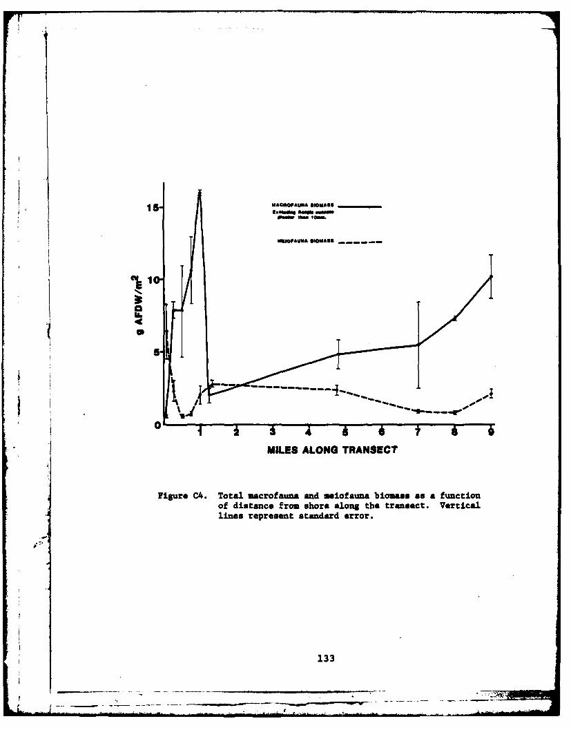
10 A40FUAOASS__
10-
5-
MILES ALONG TRANSECT
Figure C4.. Total macrofauna and aiofauna biomass as a functionof distance from shore along the transect. Verticallines represent standard error.
133

100
7-
5 -
2 -
MILES ALONG TRANSECT
Figure C5. Biomass of the claims A. cuneata compared to M.Pontchartra1iensis as a function of distance fromshore along the transect. Darkened circles show meanbiomass of R. cuneata If large clam are Included.Vertical lines represent standard error.
134
WON

6--
S 4
3
2-
0
MILES ALONG TRANSECT
Figure C6. Blomaas of the hydrobild snails P. protera compared,to T. sphinctostom as a function of distance fromshore along the transact. Vertical lines representstandard error.
1235

I
biomass were noted among the other stations (Figure C4). It is notsurprising that total biomass of meiofauna was significantly correlatedwith percent sand and shell ratio (P > 0.001), which were both highestat station 1.
Nematode species comrpised the dominant taxa at nearshore stations 1-5(Figure C7). Nematodes accounted for 82% of the meiofaunal biomass atstation 1, where the individuals were much lar er than nematodes collectedat other stations (6.0 pg vs. 2.5 pg afdw-ind 1).
At stations 6, 7, and 8, nematode biomass declined and harpacticoidcopepods became the dominant meiobenthic form (Figure C7). Copepodbiomass was found to be significantly correlated with percent clay ofthe sediments (P > 0.05). Nematodes became dominant again at stations 9and 10 near the Causeway.
Summary and Implications
The following conclusions about shell dredging effects can be drawnfrom this transect study:
(1) Peaks in total community metabolism, macrofauna biomass, andorganic carbon content were found one mile from shore, at theedge of the shoreline protected zone.
(2) Macrofauna biomass, organic carbon content, and shell contentdecreased rapidly between one mile and 1.25 miles from shore.
(3) Structure of the benthic assemblages changed markedly from theshore to the middle of the lake. At the lake edge, a varietyof relatively rare macrofaunal species occurred at low densities,along with a meiofaunal community of high biomass dominated bynematodes. From 0.25 to 1.00 miles from shore, the macrofaunawere dominated by a clam, Rangia cuneata and a hydrobiidsnail, Probythinella protera. Nematodes continued to predominatein the meiofauna. From 1.25 miles to 7.00 miles (correspondingto the active dredging zone), another clam and another snailspecies became dominant (Mulinia pontchartrainensis and Texadinasphinctostoma), and copepods became the major meiofaunal taxa.Between 7.00 miles and the end of the transect (correspondingto the Causeway protected zone) nematodes again replacedcopepods as the dominant meiofaunal taxon.
" (4) Total community metabolism, macrofauna biomass, and shellcontent increased to approximately the nearshore levels between7.00 miles and the end of the transect (9.00 miles), corre-sponding to the Causeway protected zone.
From these structural and functional data, it appears that the 10stations on the transect can be grouped into four distinct benthiccommunities: a lake edge community, a nearshore community, an open lakecommunity, and a "Causeway zone" community. Estimates of maximum dailymetabolism of these communities are: 1.17 ± 0.12 g C per m2 per day
136

% COMPOSITION-MEIOFAUNA BIOMASS
NE 0 10 20 30 40 50 60 70 80 90 100STA
NEAR-
OPEN *LAKE
CAUSE-
WAV
Figure C7. Percent composition of meiofaunal biomass in termsof dominant tax& and region in the lake.
137

(lake edge), 2.36 ± 0.65 g C per M2 per day (nearshore), 1.47 ± 0.22 g Cper m2 per day (open lake), and 1.81 ± 0.38 g C per m2 per day (Causewayzone).
Several explanations could account for these different zones:(1) Edge effects, including different regimes of hydrologic energy andvariations in sediment grain size distribution; (2) differential predationrates, i.e., enhanced predation at the lake edge and in the open lake;(3) differences in the magnitude of cultural perturbations in the foursubsystems.
The most probable explanation is a combination of 1 and 3; that is,shell dredging in the open lake, coupled with the natural enhancement ofbenthic diversity and productivity near the shore of the lake.
It should be pointed out that although station 10 is within theCauseway protected zone, it was experimentally dredged during the courseof the dredging effects study. That no significant differences betweenstations 9 and 10 showed up in this study is, therefore, somewhat anomalous,but might be explained by the fact that the three subsamples collectedat station 10 were taken exactly at the marker buoy in a spot thatremained intact following the experimental dredging. The results ofthis study would not be changed if all data from station 10 were omitted.
Literature Cited
Roberts, D. W. 1981. Structure and function of nearshore and open lakebenthic comunities in Lake Pontchartrain, Louisiana. M.S. thesis,LSU, Baton Rouge, LA.
Smith, K. L., Jr. 1973. Respiration of a sublittoral community.Ecology 54:1065-1075.
138
...

APPENDIX D
EFFECT OF SHELL DREDGING ON LAKE PONTCHARTRAINMEIOBENTHIC COPEPODS
by J. W. Fleeger
The effect of dredging did not act equally on all meiobenthiccopepod species, and thus analysis of total copepod abundance revealslittle about dredging effects. For total copepod numbers, analysis ofvariance (ANOVA) shows significant temporal, i.e., seasonal, changes indensity; however, no differences in abundance could be discerned betweenthe control and dredged sites. Analysis of individual species reveals adifferential response to dredging. Both short-term (within 50 daysfollowing dredging) and long-term (as long as 425 days following dredging)effects are discussed below for the four most abundant meiobenthiccopepods; together these four comprise more than 98% of all copepodscollected. These copepods are of the epibenthic type (see Coull 1977),living at the sediment-water interface, and all four are common frombrackish water, soft sediment locations in Louisiana (see Wilson 1958,Hiegel 1969, Fleeger and Clark 1979).
ANOVA reveals that both Scottalana canadensis, a harpacticoid, andAcarti? tonsa, a calanoid, respond in a very similar fashion to dredgingand to seasonality. These species are well known from the plankton aswell as from the benthos. Both are present in collections from eachseason, although S. canadensis does have a slight density peak in latefall, wjereas A. tonsa shows a similar peak in early fall. Short termeffects on density are shown for S. canadensis and A. tonsa by significantdensity declines within 50 days following dredging. Both species,however, recovered by the spring of 1979, and no long-term impact ondensity could be detected.
ANOVA statistics show that Halicyclops fosteri, a cyclopoid, andPseudobradya sp., a harpacticoid, have distinct seasonal trends inpopulation density. Both species are also found in the plankton, butwith much less repularity compared to Scottolana canadensis and Acartiatonsa. H. fosteri displayed a pronounced density peak in early Augustof 1978 and 1979, with a marked population decline in late August andearly September. Psuedobradya sp. was prominent only in spring collec-tions and was the dominant copepod from February-April 1979.
Long-term dredging effects are shown by ANOVA for H. fosteri andPseudobradya sp. A dramatic seasonal (August) decline in H. fosteriabundance took place concurrently with the initial dredging, makingidentification of short-term dredging effects on K. fosteri impossible.H. fosteri did recover at the dredged site by the spring of 1979, and,in fact, long-term trends reveal a significantly greater abundance atthe dredged site compared to the control during August 1979. During thefollowing year, the dredged and control sites were similar in abundancefor H. fn-teri. Short-term dredging effects on Pseudobradya sp. areimpossible -o detect because of its low seasonal abundance when dredgingtook place in the fall of 1978. A long-term effect occurred as densitiesof Pseudobradya sp. were increased at the dredged site relative to the
139
.. . . ...

control during the spring of 1979. During 1980, Pseudobradya sp. abun-dances were similar at each site.
To summarize, Scottolana canadensis and Acartia tonsa showed short-term impacts attributable to shell dredging. Both species recoveredwithin six months, and no long-term effect was observed. For Halicyclopsfosteri and Pseudobradya sp., no short-term effects of dredging weredetected because of the presence of seasonal effects. Long-term effectson both species were evident. H. fosteri showed increased abundance atthe dredged site one year after dredging; however, no differences wereseen after two years. In Pseudobradya sp., increased abundance wasobserved after 6-8 months at the dredged site. Following this increase,dredged and control sites showed equal densities.
Table Dl. Summary of ANOVA statistics calculated on copepod abundances.
Short-Term Long-Term
Seasonal Dredging vs. Seasonal Dredging vs.Species Trends Control Trends Control
Halicyclops fosteri + - + +
Pseudobradya sp. + - + +
Scottolana canadensis + + +.
Acartia tonsa + + +
Short-term refers to the 50 day period following dredging, long-term tothe entire 425 days currently under investigation. A + indicatessignificance at the 0.05 level of probability; a - indicates a probabilityvalue greater than 0.05.
Literature Cited
Coull, B. C. 1977. Marine flora and fauna of the Northeastern United States.Copepoda: Harpacticoida. NOAA Tech. Rep. NHFS Circular 399. pp. 1-48.
Fleeger, J. W., and D. R. Clark. 1979. A revised key to Leptocaris(Copepoda: Harpacticoida), including a new species from a shallowestuarine lake in Louisiana, USA. Northeast Gulf Sci. 3:53-59.
Hiegel, M. H. 1969. A survey of the bottom dwelling copepods of a Louisianamarsh lake. M.S. Thesis, Louisiana State University, Baton Rouge,pp. 1-109.
Wilson, H. S. 1958. The copepod genus Halicyclops in North America, witha description of a new species from Lake Pontchartrain, Louisiana,and the Texas Coast. Tulane Stud. Zool. 6:176-189.
140

DATE
FILME