JHEP08(2018)149

Published for SISSA by Springer

Received: July 19, 2018

Accepted: August 17, 2018

Published: August 23, 2018

Antisymmetric Wilson loops in N = 4 SYM: from

exact results to non-planar corrections

Anthonny F. Canazas Garay,a Alberto Faraggib and Wolfgang Muckc,d

aInstituto de Fısica, Pontificia Universidad Catolica de Chile,

Casilla 306, Santiago, ChilebDepartamento de Ciencias Fisicas, Facultad de Ciencias Exactas, Universidad Andres Bello,

Sazie 2212, Piso 7, Santiago, ChilecDipartimento di Fisica “Ettore Pancini”, Universita degli Studi di Napoli “Federico II”,

via Cintia, 80126 Napoli, ItalydIstituto Nazionale di Fisica Nucleare, Sezione di Napoli,

via Cintia, 80126 Napoli, Italy

E-mail: afcanazas@uc.cl, alberto.faraggi@unab.cl,

wolfgang.mueck@na.infn.it

Abstract: We consider the vacuum expectation values of 1/2-BPS circular Wilson loops

in N = 4 super Yang-Mills theory in the totally antisymmetric representation of the gauge

group U(N) or SU(N). Localization and matrix model techniques provide exact, but rather

formal, expressions for these expectation values. In this paper we show how to extract the

leading and sub-leading behavior in a 1/N expansion with fixed ’t Hooft coupling starting

from these exact results. This is done by exploiting the relation between the generating

function of antisymmetric Wilson loops and a finite-dimensional quantum system known

as the truncated harmonic oscillator. Sum and integral representations for the 1/N terms

are provided.

Keywords: 1/N Expansion, AdS-CFT Correspondence, Matrix Models, Wilson, ’t Hooft

and Polyakov loops

ArXiv ePrint: 1807.04052

Open Access, c© The Authors.

Article funded by SCOAP3.https://doi.org/10.1007/JHEP08(2018)149

JHEP08(2018)149

Contents

1 Introduction 1

2 Gaussian matrix model 3

2.1 Partition function and expectation values 3

2.2 Properties of the matrix I(y, z) 5

2.3 Truncated harmonic oscillator 6

2.4 Generating function 8

3 Wilson loops at leading order 10

4 Wilson loops at next-to-leading order 12

4.1 Matrix elements 12

4.2 Powers of I(g, g) and their traces 15

4.3 Generating function 17

4.4 Holographic regime 18

5 Conclusions 21

A Some properties of the Hermite polynomials 22

B Trace of normal ordered products 23

C Conversion of the sum over the roots of HeN to an integral 24

D Proof of (4.16) 25

E Proof of (4.29) 26

1 Introduction

Wilson loop operators have played a central role in the development of gauge/gravity

dualities [1, 2]. In this context, the 12 -BPS circular loop in N = 4 super Yang-Mills theory

with U(N) and SU(N) gauge groups and ’t Hooft coupling λ has received special attention,

mainly due to the conjecture put forward in [3, 4] that its expectation value is captured

exactly, to all orders in N and λ, by a Gaussian matrix model. This conjecture was

later proved in [5] using supersymmetric localization, a technique that has since provided

theorists with a several other exact results in supersymmetric gauge theories. These include,

for example, Wilson loops preserving less supersymmetry [6–10], correlators of Wilson loops

with chiral primary operators [11–18], correlators between Wilson loops [19], as well as

Wilson loops and their correlators in N = 2 super Yang-Mills theory [20–26].

– 1 –

JHEP08(2018)149

A key ingredient in the description of Wilson loop operators is the representation of the

gauge group, typical ones for U(N) and SU(N) being the fundamental, totally symmetric

and totally antisymmetric representations. Depending on the rank of the representation,

the holographic dual corresponds to probe strings or D-branes [27, 28] propagating on

AdS5 × S5, or to fully back-reacted bubbling geometries [29–32]. In all cases, the on-shell

action of the gravitational object agrees perfectly with the matrix model calculation [33] at

leading order in 1/N and 1/√λ. We expect, however, that a thorough examination should

yield a match at the next-to-leading order as well. It is then crucial to systematically

extract these corrections on both sides of the duality.

From the gravitational perspective the calculation of sub-leading corrections amounts

to analyzing semi-classical fluctuations of the background configurations and computing

the corresponding one-loop partition functions. There has been considerable effort in this

direction [34–44], although the calculations are plagued with ambiguities inherent to string

theory in curved spaces.

On the gauge theory side, solving the matrix model is a non-trivial task, and comput-

ing sub-leading corrections is a conceptually clear, albeit technically difficult procedure.

Recently, sub-leading corrections in 1/N to the Wilson loop in the totally antisymmet-

ric representation have been found using loop equation techniques [45] and topological

recursion in the Gausssian matrix model [46] (see also [47] for the case of symmetric repre-

sentations). A particularly interesting development was reported in [48], where the authors

managed to compute the exact vacuum expectation value of the circular Wilson loop in

arbitrary irreducible representations using the method of orthogonal polynomials. In other

words, they solved the matrix model exactly. While useful for some purposes, their results

are rather formal, and it is not at all obvious how to extract the large-N (and large-λ)

limit from them, much less any sub-leading corrections, except for simple cases. So far,

they have only been used for numerical comparison with other approaches.

In this paper, we address and solve the problem of extracting the leading and first sub-

leading terms in the 1/N expansion of the generating function of totally antisymmetric

Wilson loops starting from the exact results in [48]. Our motivation is two-fold. First, it

is obviously interesting to see how it can be done. Second, the techniques used in [45, 46]

solve the matrix model in the continuum limit, in which the discrete poles of the matrix

model resolvent give rise to a cut singularity and a continuous eigenvalue density. In other

words, the analyticity properties of the resolvent change in this limit, and it would be

interesting to see whether and where this has any implications. We anticipate that we do

not find any at order 1/N .

The paper is organized as follows. In section 2, we review the Gaussian matrix model

and reproduce the formal result of [48] for the generating function of antisymmetric Wilson

loops. At the same time, we establish a connection with the algebra of the truncated

harmonic oscillator, which will be crucial for our developments. In section 3, we extract

the leading large-N behaviour (fixed λ) of the generating function from the formal solution

of the matrix model. The most substantial part of the paper is section 4, which contains

the calculation of the 1/N terms of the Wilson loop generating function, both for general λ

and in the holographic regime of large λ. Our results are shown to agree with [45, 46], but

– 2 –

JHEP08(2018)149

turn out to be somewhat simpler in their final form. Section 5 contains the conclusions.

Some technical details are deferred to the appendices.

2 Gaussian matrix model

Localization techniques [5] map the expectation value of the circular Wilson loop in N = 4

SYM with gauge group U(N) to an expectation value in a Gaussian matrix model. We

begin this section by reviewing this model and developing some results that will be relevant

for what follows.

2.1 Partition function and expectation values

The Gaussian matrix model is defined by the partition function

Z =

∫[dX] exp

(−2N

λTr(X2))

, (2.1)

where X is a N ×N hermitian matrix. If the gauge group is SU(N) the matrices are also

traceless, condition that can be implemented with a Lagrange multiplier. The expectation

value of any quantity F (X) in the Hermitian ensemble is then given by

〈F (X)〉 =1

Z

∫[dX]F (X) exp

(−2N

λTr(X2))

. (2.2)

When F is invariant under similarity transformations, i.e., F (V XV −1) = F (X), one can

diagonalize the matrix X in terms of its eigenvalues xn, n = 1, . . . , N , and integrate out

the remaining “angular” variables. This yields

〈F (X)〉 =1

Z

∫ [ N∏m=1

dxm

]∆2(x)F (x) exp

(−2N

λ

N∑n=1

x2n

), (2.3)

where the transformation Jacobian

∆(x) = det[xn−1m

]=

∣∣∣∣∣∣∣∣∣∣1 x1 x21 · · · x

N−11

1 x2 x22 · · · xN−12

......

.... . .

...

1 xN x2N · · · xN−1N

∣∣∣∣∣∣∣∣∣∣(2.4)

is known as the Vandermonde determinant.

The Vandermonde determinant enjoys several properties that we can exploit to our

advantage. For example, one can show that

∆(x) =∏

1≤m<n≤N|xn − xm| ⇒ ∆(x+ y) = ∆(x) , ∆(αx) = α

N(N−1)2 ∆(x) ,

(2.5)

so ∆(x) is invariant under uniform translations and transforms simply under rescalings.

Another key observation is that, up to an overall constant, the Vandermonde determinant

is the same as

∆(x) = det [Pn−1(xm)] = CN∆(x) , CN =N−1∏n=0

hn , (2.6)

– 3 –

JHEP08(2018)149

where Pn(x) = hnxn + · · · is any family of polynomials that can be chosen to our conve-

nience. Using these facts, the partition function may be written as

Z = C−2N gN2

∫ [ N∏m=1

dxm

]∆(x+ y)∆(x+ z) exp

(−1

2

N∑n=1

x2n

). (2.7)

Here, y and z are arbitrary constants, and the coupling g is defined by

g =

√λ

4N. (2.8)

We now introduce a quantity that will play a central role in our analysis of the circular

Wilson loop. Let us define the N ×N matrix

Imn(y, z) =

∫ ∞−∞

dxPm−1(x+ y)Pn−1(x+ z)e−12x2 . (2.9)

Although this definition might seem spurious at this point, its relevance will become clear

momentarily. Writing the determinant (2.6) explicitly as

∆(x) =∑

m1, ...,mN

εm1···mNPm1−1(x1) · · ·PmN−1(xN ) , (2.10)

we find that

Z = C−2N gN2N ! det [I(y, z)] . (2.11)

The same procedure can be applied to the matrix model expectation values (2.2), which

become

〈F (X)〉 =1

N ! det I(y, z)

∫ [ N∏m=1

dxm

]∆(x+y)∆(x+z)F (gx) exp

(−1

2

N∑n=1

x2n

). (2.12)

We emphazise that the integrals are independent of y and z by virtue of (2.5).

It should not come as a surprise that a very convenient choice of polynomials is

Pn(x) =Hen(x)

(2π)14

√n!, (2.13)

where Hen(x) are Hermite polynomials.1 The family Pn(x) is then orthonormal with respect

to the Gaussian weight, namely,∫ ∞−∞

dxPm(x)Pn(x) e−12x2 = δmn . (2.14)

Furthermore, the matrix elements (2.9) can be computed explicitly [49], yielding

Imn(y, z) =

√(n− 1)!

(m− 1)!ym−n L

(m−n)n−1 (−yz) =

√(m− 1)!

(n− 1)!zn−m L

(n−m)m−1 (−yz) , (2.15)

where L(α)n (x) are Laguerre polynomials. Owing to the properties of these polynomials, the

distinction between the cases m ≥ n and m < n is not necessary.

1Even though we are physicists, we work with the probabilists’ version of the Hermite polynomials in

order to avoid some awkward factors of√

2. Some basic properties of the Hermite polynomials are listed

in appendix A.

– 4 –

JHEP08(2018)149

2.2 Properties of the matrix I(y, z)

We now proceed to discuss some noteworthy attributes of the matrix (2.15). First, one

easily verifies that

I(0, 0) = 1 , (2.16)

IT (y, z) = I(z, y) , (2.17)

I(ξy, ξ−1z) = P (ξ)I(y, z)P−1(ξ) , Pmn(ξ) = ξmδmn . (2.18)

Moreover, I(y, 0) and I(0, z) are lower and upper triangular matrices, respectively, with

unit diagonal entries. Thus, det I(y, 0) = det I(0, z) = 1. Some algebra shows that I(y, z)

has the LU decomposition

I(y, z) = I(y, 0)I(0, z) . (2.19)

It immediately follows that

det I(y, z) = 1 . (2.20)

The matrix also satisfies

I(y1, 0)I(y2, 0) = I(y1 + y2, 0) , (2.21)

which, combined with (2.17) and (2.19), implies

I(y1 + y2, z1 + z2) = I(y2, 0)I(y1, z1)I(0, z2) . (2.22)

We also deduce that

I−1(y, z) = I(0,−z)I(−y, 0) . (2.23)

Furthermore, I(y, z) is similar to its inverse, because

I−1(y, z) = [P (−1)I(0, z)] I(y, z) [P (−1)I(0, z)]−1 , (2.24)

as can be shown using (2.18), (2.19) and (2.23). This implies that the eigenvalues of I(y, z)

come in reciprocal pairs and that its characteristic polynomial is either palindromic or

anti-palindromic.

The properties (2.21) are reminiscent of an exponential behavior. This is no coinci-

dence. Indeed, one can verify the remarkable relation

I(0, z) = ezA ⇒ I(y, z) = eyAT

ezA , (2.25)

where A is the matrix given by

An,n+1 =√n , (2.26)

and all other entries vanishing. More explicitly,

A =

0√

1 0 · · · 0

0 0√

2 · · · 0...

......

. . ....

0 0 0 · · ·√N − 1

0 0 0 · · · 0

. (2.27)

Note that any power of A is traceless and that AN = 0. The same is true for AT , of course.

– 5 –

JHEP08(2018)149

2.3 Truncated harmonic oscillator

We promptly notice that A and AT are nothing more than the matrix representation of

the ladder operators of the harmonic oscillator truncated to the first N energy eigenstates.

Surely, the number operator

N = ATA =

0 0 0 · · · 0

0 1 0 · · · 0

0 0 2 · · · 0...

......

. . ....

0 0 0 · · · N − 1

(2.28)

is diagonal and satisfies

[N , A] = −A , [N , AT ] = AT . (2.29)

However, A and AT themselves do not fulfill the Heisenberg algebra. Instead, their com-

mutator reads

[A,AT ] = 1−N diag (0, . . . , 0, 1) , (2.30)

which is traceless, as must be for finite-dimensional operators.

The N -dimensional quantum mechanical system formed by the operators A and AT ,

chiefly called the truncated harmonic oscillator, is well known in quantum optics. We recall

here some of its properties, following the recent account [50] and refer the interested reader

to more references in that paper. In the next sections we will exploit this connection to

the truncated harmonic oscillator in order to extract the leading and sub-leading large N

behavior of the circular Wilson loops.

In a fairly obvious notation, we denote by |n〉, n = 0, 1, . . . , N − 1 the column vector

with a 1 in the n + 1-th position and zeros elsewhere. These states are eigenstates of the

number operator N and whence are called the number basis. According to (2.27), the

ladder operators act upon them as

A|n〉 =√n|n− 1〉 n = 0, 1, . . . , N − 1 , (2.31)

AT |n〉 =√n+ 1|n+ 1〉 n = 0, 1, . . . , N − 2 , AT |N − 1〉 = 0 . (2.32)

Of course, the matrix elements (2.15) are

Imn(y, z) = 〈m| eyAT ezA |n〉 . (2.33)

Actually, this same expression can be obtained by computing the matrix elements of the

displacement operator D(y, z) = eya†eza = e

yz2 eya

†+za in the full, infinite-dimensional,

quantum harmonic oscillator [51], and then truncating to the first N number states.

We will now construct a basis for the N -dimensional Hilbert space which is more suited

to our purposes. Consider the states

|ζ〉 =N−1∑n=0

Hen(ζ)√n!|n〉 , (2.34)

– 6 –

JHEP08(2018)149

where ζ is an arbitrary real parameter. By virtue of the recursion relations for the Hermite

polynomials, the actions of A and AT on |ζ〉 can be formally represented as

A|ζ〉 =

(ζ − ∂

∂ζ

)|ζ〉 − HeN (ζ)√

(N − 1)!|N − 1〉 , (2.35)

AT |ζ〉 =∂

∂ζ|ζ〉 . (2.36)

We see that |ζ〉 is an approximate eigenstate of A+AT . It becomes an exact eigenstate if

ζ is a root of HeN , (A+AT

)|ζ〉 = ζ|ζ〉 , if HeN (ζ) = 0 . (2.37)

This construction makes explicit the fact that A+AT is actually the companion matrix of

the Hermite polynomial of degree N , namely,

det[ζ −

(A+AT

)]= HeN (ζ) . (2.38)

Now, the Hermite polynomial HeN (ζ) has precisely N distinct roots, which we denote

in increasing order by ζi, i = 1, 2, . . . , N . One can show that the corresponding states |ζi〉are linearly independent by computing their inner product with the aid of the Christoffel-

Darboux formula,

〈η|ζ〉 =N−1∑n=0

Hen(η) Hen(ζ)

n!=

1

(N − 1)!

HeN (η) HeN−1(ζ)−HeN (ζ) HeN−1(η)

η − ζ. (2.39)

Then,

〈ζi|ζj〉 = c2i δij , ci =HeN+1(ζi)√

N !, (2.40)

and the vectors |ζi〉 form an orthogonal basis of the Hilbert space called the position basis.

The matrix elements of I(y, z) in the position basis are

Iij(y, z) =1

cicj〈ζi| eyA

TezA |ζj〉 . (2.41)

We will use this expression extensively in the next sections. Before we move on, we would

like to point out that it is possible to write an exact expression for I−1(y, z) that takes a

particularly simple form. Indeed, since AT acts on |ζ〉 as a derivative, we have

I−1ij (y, z) =1

cicj〈ζi| e−zA e−yA

T |ζj〉

=1

cicj〈ζi − z|ζj − y〉 . (2.42)

Even though we will not use this formula in what follows, we believe that it could lead to

some simplifications in the analysis of sub-leading corrections to the expectation value of

the circular Wilson loop.

– 7 –

JHEP08(2018)149

2.4 Generating function

The precise relation between the circular Wilson loop and the Gaussian matrix model is

〈WR〉U(N) =1

dim[R]

⟨TrR

[eX]⟩, (2.43)

where R denotes the representation of the U(N) gauge group and TrR the corresponding

trace. The vacuum expectation value on the left is defined on the N = 4 SYM theory; the

right hand side corresponds to an insertion in the matrix model.

In this paper we will be concerned with the totally antisymmetric representation of

rank k defined by the Young diagram

Ak = ...

k . k ≤ N . (2.44)

It has dimension

dim[Ak] =

(N

k

). (2.45)

The structure of the trace TrAk can get increasingly complicated as the rank k grows.

Indeed, for any N ×N matrix X we have

TrA1 X = TrX , (2.46)

TrA2 X =1

2(TrX)2 − 1

2Tr(X2), (2.47)

TrA3 X =1

6(TrX)3 − 1

2Tr(X2)

TrX +1

3Tr(X3), (2.48)

and so forth. Happily, there is a natural way to encode this structure into the generating

function

FA(t;X) ≡ det [1 + tX] =N∑k=0

tk TrAk [X] . (2.49)

A straightforward calculation using (2.9), (2.10) and (2.12) reveals that the matrix

model expectation value of this generating function is

⟨FA(t; eX)

⟩U(N)

= det

[I(y, z) + t e

g2

2 I(g + y, g + z)

]= det

[1 + t e

g2

2 I(g, g)

], (2.50)

where the matrix I(g, g) was introduced in (2.15). The dependence on y and z disappears as

a consequence of (2.21) and (2.20). This is essentially the answer reported by Fiol and Tor-

rents in [48], except that they use a slightly different matrix, which we call I(g, g), obtained

from I(g, g) by multiplying the m-th row by√

(m− 1)! g−m and dividing the m-th column

by the same factor. The determinant in (2.50) does not change under these operations, so⟨FA(t; eX)

⟩U(N)

= det[1 + t e

12g2 I(g, g)

], Imn(g, g) = L

(m−n)n−1 (−g2) , (2.51)

– 8 –

JHEP08(2018)149

which is the expression given in [48]. Note also that our generating functional differs by a

factor of tN from theirs.

In the answer (2.50) we recognize the form of the generating function of antisymmetric

traces (2.49) for the matrix I(g, g),⟨FA(t; eX)

⟩= FA

(t e

λ8N ; I(g, g)

), (2.52)

which allows us, using (2.49) and (2.43), to obtain the formal yet remarkably simple result

〈WAk〉U(N) =1

dim[Ak]eλk8N TrAk [I(g, g)] . (2.53)

For the gauge group SU(N), the matrix model must be restricted to traceless matrices.

This can be achieved either by using a Lagrange multiplier or by explicitly isolating the

trace component in the matrix model integral, as was done in [45]. The outcome is

〈WAk〉SU(N) = 〈WAk〉U(N) e−λk2

8N2 =1

dim[Ak]eλk(N−k)

8N2 TrAk [I(g, g)] . (2.54)

Because the representations Ak and AN−k are conjugate to each other for the gauge group

SU(N), we expect 〈WAk〉SU(N) =⟨WAN−k

⟩SU(N)

. This can be demonstrated by noting

that, for an invertible matrix X, (2.49) implies

TrAN−k [X] = det[X] TrAk [X−1] . (2.55)

Now, since I(g, g) is similar to its inverse, and det I(g, g) = 1, this gives

TrAN−k [I(g, g)] = TrAk [I(g, g)] , (2.56)

which proves the assertion. Equation (2.56) also shows that the generating function

FA(t; I(g, g)) is a palindromic polynomial.

The main object of study in the remainder of this paper is the function

F(t) =1

NlnFA(t; I(g, g)) =

1

NTr ln[1 + tI(g, g)] , (2.57)

from which the traces TrAk [I(g, g)] can be calculated by

TrAk [I(g, g)] =

∮dt

2πiteN [F(t)−κ ln t] , (2.58)

where we have introduced the ratio

κ =k

N. (2.59)

We are interested in the large N regime, keeping the ’t Hooft coupling λ and the ratio κ

fixed. In this regime, the integral in (2.58) is dominated by the saddle point value,2

TrAk [I(g, g)] = eN [F(t∗)−κ ln t∗]− 12ln[2πN(κ+t2∗F ′′(t∗))] , (2.60)

2To obtain (2.60), introduce t = t∗ eiz, expand the integrand in z up to second order and evaluate the

Gaussian integral. The second term in the exponent comes from the Gaussian integral.

– 9 –

JHEP08(2018)149

where t∗ satisfies the saddle point equation

t∗F ′(t∗) = κ . (2.61)

Moreover, F(t) admits an asymptotic expansion in 1/N ,

F(t) =∞∑n=0

FnN−n . (2.62)

Our aim is to calculate the terms F0(t) and F1(t) from the exact, but formal, expres-

sion (2.57).

3 Wilson loops at leading order

In this section, we shall calculate the leading order term F0(t) of the generating function.

Of course, F0(t) is known both from a matrix model calculation and from the holographic

dual [28, 33] (the latter implying large λ in addition to large N). Here, we reproduce

it starting from the exact expression (2.57) by means of two different calculations, which

exploit the relation of the matrix I to the truncated harmonic oscillator.

Let us start in the number basis. This calculation will lead to the expression for F0(t)

that Okuyama [46] attributes to an unpublished note by Beccaria. Starting from (2.57)

and Taylor-expanding the logarithm we may write

F(t) = − 1

N

∞∑n=1

(−t)n

nTr[I(g, g)n] . (3.1)

In order to compute the powers of the matrix I(g, g) we resort to the representation (2.25).

To leading order in 1/N , commutators of the matrices A and AT can be neglected, so that

we can essentially normal order the product in the trace. This leads to

F(t) = −∞∑n=1

(−t)n

n

1

NTr(

engAT

engA)

+O(1/N) . (3.2)

We can now expand the exponentials and calculate the traces. We defer this little calcula-

tion to appendix B. With the results (B.3) and (B.5), this yields

F(t) = −∞∑n=1

(−t)n

n

N−1∑k=0

(ng)2k

k!(k + 1)!

(N − k)k+1

N. (3.3)

The leading term in 1/N is found to be

F0(t) = −∞∑n=1

(−t)n

n

∞∑k=0

(n√λ/2)2k

k!(k + 1)!= − 2√

λ

∞∑n=1

(−t)n

n2I1(n√λ) , (3.4)

where I1(x) denotes a modified Bessel function. This is precisely J0 in (2.21) of [46].

– 10 –

JHEP08(2018)149

A slightly simpler way of arriving at (3.4) is to recognize (3.2) as

F(t) = −∞∑n=1

(−t)n

n

1

NTr[I(ng, ng)] +O(1/N) . (3.5)

The trace follows easily from (2.15) and the identity [52]

N∑m=1

L(α)m−1(x) = L

(α+1)N−1 (x) . (3.6)

Hence, (3.5) becomes

F(t) = −∞∑n=1

(−t)n

n

1

NL(1)N−1(−n

2g2) +O(1/N) . (3.7)

For large order, the Laguerre polynomials satisfy [52]

limN→∞

1

NαL(α)N

(− z

N

)=

1

zα2

Iα

(2z

12

), (3.8)

with Iα(x) being a modified Bessel function. Recalling that g =√

λ4N , applying the

limit (3.8) to (3.7) gives (3.4).

For a comparison with the matrix model calculation in the saddle point approxima-

tion [33], one can use the following integral representation of the modified Bessel func-

tion [52],

I1(z) =z

π

π∫0

ez cos θ sin2 θ dθ . (3.9)

After substituting (3.9) into (3.4), the summation can be carried out to give

F0 =2

π

π∫0

dθ sin2 θ ln(

1 + t e√λ cos θ

). (3.10)

A simple change of variables transforms this integral into the one in (2.26) of [33].

The computation of F0(t) turns out to be considerably simpler in the position basis.

The reason for this is that, to leading order in 1/N , we can also write

I(g, g) = eg(A+AT ) +O(1/N) , (3.11)

where all commutators in the Baker-Campbell-Hausdorff formula contribute to the O(1/N)

terms. According to (2.37), the operator in the exponential is diagonal in the position basis,

so that (2.57) simply becomes

F(t) =1

N

N∑i=1

ln(

1 + t egζi)

+O(1/N) . (3.12)

– 11 –

JHEP08(2018)149

The sum is taken over the roots of the Hermite polynomial HeN (ζ). For large N , the

distribution of zeros becomes dense and is described by the Wigner semi-circle law. Us-

ing formulas (A.11) and (A.12) to determine the integral measure and dropping the 1/N

contributions, we get

F0(t) =2

π

∫ π

0dθ sin2 θ ln

(1 + t e

√λ cos θ

), (3.13)

which agrees with (3.10).

4 Wilson loops at next-to-leading order

In this section, we extend the calculation of the generating function F(t) to order 1/N , i.e.,

we obtain the subleading term F1(t) in the expansion (2.62). Our results agree with [46],

although we also managed to make a slight simplification. In the holographic regime of

large λ, we will find agreement with [45].

Exploiting the relation between the matrix I(g, g) in the position basis and the zeros

of Hermite polynomials appears to be the most promising path to compute the subleading

corrections. Starting again from (3.1), we will proceed as follows. In subsection 4.1, we

compute the matrix elements of I(g, g) in the position basis up to order 1/N , which results

in an expression like

I(g, g) = I(0) +1

NI(1) +O(1/N2) . (4.1)

The leading term I(0) is known from the calculation at the end of the previous section and

is diagonal. The main effort in subsection 4.1 consists in finding I(1). We then need to

compute powers of I(g, g). This is not as straightforward as one might think because I(1)

is a dense matrix. Consider, for example,

I2(g, g) = [I(0)]2 +1

N

[I(0)I(1) + I(1)I(0)

]+

1

N2[I(1)]2 . (4.2)

The last term, which naively seems to be of order 1/N2, is, in fact, of order 1/N , because

the matrix multiplication contains a sum over N terms of order 1. The same happens for

higher powers. The calculation of the powers of I(g, g) and their traces will be done in

subsection 4.2. Another source of 1/N contributions is the conversion of the sum over the

roots of Hermite polynomials, which label the position basis elements, into an integral. We

present the details of this conversion in appendix C. The generating function F(t) will be

calculated in subsection 4.3, where we will also provide its integral representation. Finally,

in subsecion 4.4, we consider F1(t) in the holographic regime of large λ.

4.1 Matrix elements

Consider the matrix I(g, g) = egA†

egA. With |ζ〉 defined in (2.34), we find by direct

application of the properties (2.31) and (2.32)

egA†

egA |ζ〉 =

N−1∑k=0

N−1∑l=0

min(N−1,N−1−l+k)∑n=0

gk+l

k!l!

(n

k

)k!

Hen+l−k(ζ)√n!

|n〉 . (4.3)

– 12 –

JHEP08(2018)149

0

n

0 N− 1−n ∞

N− 1

k

↓

l →

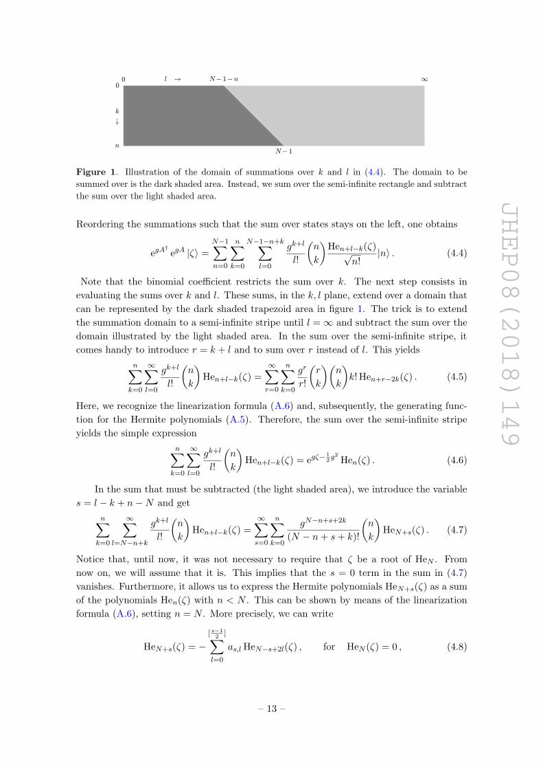
Figure 1. Illustration of the domain of summations over k and l in (4.4). The domain to be

summed over is the dark shaded area. Instead, we sum over the semi-infinite rectangle and subtract

the sum over the light shaded area.

Reordering the summations such that the sum over states stays on the left, one obtains

egA†

egA |ζ〉 =

N−1∑n=0

n∑k=0

N−1−n+k∑l=0

gk+l

l!

(n

k

)Hen+l−k(ζ)√

n!|n〉 . (4.4)

Note that the binomial coefficient restricts the sum over k. The next step consists in

evaluating the sums over k and l. These sums, in the k, l plane, extend over a domain that

can be represented by the dark shaded trapezoid area in figure 1. The trick is to extend

the summation domain to a semi-infinite stripe until l =∞ and subtract the sum over the

domain illustrated by the light shaded area. In the sum over the semi-infinite stripe, it

comes handy to introduce r = k + l and to sum over r instead of l. This yields

n∑k=0

∞∑l=0

gk+l

l!

(n

k

)Hen+l−k(ζ) =

∞∑r=0

n∑k=0

gr

r!

(r

k

)(n

k

)k! Hen+r−2k(ζ) . (4.5)

Here, we recognize the linearization formula (A.6) and, subsequently, the generating func-

tion for the Hermite polynomials (A.5). Therefore, the sum over the semi-infinite stripe

yields the simple expression

n∑k=0

∞∑l=0

gk+l

l!

(n

k

)Hen+l−k(ζ) = egζ−

12g2 Hen(ζ) . (4.6)

In the sum that must be subtracted (the light shaded area), we introduce the variable

s = l − k + n−N and get

n∑k=0

∞∑l=N−n+k

gk+l

l!

(n

k

)Hen+l−k(ζ) =

∞∑s=0

n∑k=0

gN−n+s+2k

(N − n+ s+ k)!

(n

k

)HeN+s(ζ) . (4.7)

Notice that, until now, it was not necessary to require that ζ be a root of HeN . From

now on, we will assume that it is. This implies that the s = 0 term in the sum in (4.7)

vanishes. Furthermore, it allows us to express the Hermite polynomials HeN+s(ζ) as a sum

of the polynomials Hen(ζ) with n < N . This can be shown by means of the linearization

formula (A.6), setting n = N . More precisely, we can write

HeN+s(ζ) = −[ s−1

2]∑

l=0

as,l HeN−s+2l(ζ) , for HeN (ζ) = 0 , (4.8)

– 13 –

JHEP08(2018)149

with coefficients as,l, which satisfy

m∑k=0

(s

k

)(N

k

)k!as−2k,m−k =

(s

m

)(N

s−m

)(s−m)! . (4.9)

The coefficients as,l can be determined applying (4.9) recursively for increasing m. The

first steps of this recursion yield

as,0 =

(N

s

)s! , as+2,1 = −

(N

s

)s!s(s+ 2) , . . . . (4.10)

We shall not investigate this recursion further, because it will turn out that only as,0 is

relevant for our purposes. After substituting (4.8) into (4.7), we can reorder the summations

over s and l by introducing r = s− 2l and obtain

−∞∑s=0

n∑k=0

gN−n+s+2k

(N − n+ s+ k)!

(n

k

) [ s−12

]∑l=0

as,l HeN−s+2l(ζ) =

= −n∑k=0

N∑r=1

(n

k

)HeN−r(ζ)

∞∑l=0

gN−n+r+2l+2k

(r +N − n+ 2l + k)!ar+2l,l . (4.11)

With these results, let us now consider the matrix element of egA†

egA between two

(non-normalized) position eigenstates. Remember that the sum over k and l in (4.4) is

given by (4.6) minus (4.11). We find

〈ζi| egA†

egA |ζj〉 = egζj−12g2〈ζi|ζj〉 (4.12)

+

N∑r,s=1

HeN−s(ζi) HeN−r(ζj)∞∑k=0

∞∑l=0

gr+s+2(l+k)ar+2l,l

k!(N − s− k)!(s+ r + 2l + k)!.

where we have used the definition of the states |ζ〉 (2.34), extended the summation over k

(this can be done because of the binomial) and let s = N − n. Furthermore, rewriting the

sums over l and k as a sum over n = l + k and k gives

〈ζi| egA†

egA |ζj〉 = egζj−12g2〈ζi|ζj〉 (4.13)

+

N∑r,s=1

HeN−s(ζi) HeN−r(ζj)

∞∑n=0

gr+s+2n

(r + s+ 2n)!

n∑k=0

(r + s+ 2n

k

)ar+2(n−k),n−k

(N − s− k)!.

In the first term on the right hand side, one can recognize the leading order result, corrected

by the exponential e−12g2 . Therefore, the second term is of order 1/N , so that leading order

relations can be used to manipulate it. A short inspection of the sum over k in (4.13) for

some low values of n shows that the leading order contribution in 1/N comes from the

term with k = n. Therefore, using (4.10), we get

n∑k=0

(r + s+ 2n

k

)ar+2(n−k),n−k

(N − s− k)!∼(r + s+ 2n

n

)N !(N − s− n+ 1)n

(N − r)!(N − s)!

∼(r + s+ 2n

n

)N !Nn

(N − r)!(N − s)!, (4.14)

– 14 –

JHEP08(2018)149

where subleading terms in 1/N have been omitted. Then, after normalizing the matrix

elements (4.13) by means of (2.40) and substituting (4.14), we obtain

Iij(g, g) = egζj−12g2 δij (4.15)

+

N∑r,s=1

(N !)2

(N − r)!(N − s)!HeN−s(ζi) HeN−r(ζj)

HeN+1(ζi) HeN+1(ζj)

∞∑n=0

gr+s+2nNn

(r + s+ n)!n!+O

(1

N2

).

It is possible to obtain simple expressions for the ratios HeN−s(ζi)/HeN+1(ζi). We

include the calculation in appendix D, where we show that, to leading order in 1/N ,

HeN−s(ζ)

HeN+1(ζ)∼ −(N − s)!

N !N

s−12 Us−1(cos θ) , (4.16)

where cos θ is determined by ζ ∼ 2√N cos θ, and Us denote the Chebychev polynomials of

the second kind [49],

Us(cos θ) =sin[(s+ 1)θ]

sin θ. (4.17)

Hence, we obtain our final result for the matrix I(g, g) in the position basis,

Iij(g, g) = egζj−12g2 δij +

1

N

N∑r,s=1

sin(sθi) sin(rθj)

sin θi sin θj

∞∑n=0

(√λ/2)r+s+2n

(r + s+ n)!n!+O

(1

N2

)(4.18)

= e−λ8N e

√λ√

1+ 12N

cos θi δij +1

N

∞∑r,s=1

sin(sθi) sin(rθj)

sin θi sin θjIr+s(

√λ) +O

(1

N2

).

In the step from the first to the second line we have recognized the modified Bessel functions

in the sums over n and expressed the roots ζi in the diagonal term in terms of cos θi being

careful to use the expression (A.11), which is exact to order 1/N .3 Moreover, we have

extended the summations to infinity in the sense of an asymptotic expansion.

4.2 Powers of I(g, g) and their traces

In this subsection, we return to calculate the quantities needed in the generating func-

tion (3.1), namely the powers of the matrix I(g, g) and their traces. As mentioned at the be-

ginning of this section, calculating the powers of I(g, g) to order 1/N is not straightforward.

Fortunately, after calculating a few powers, e.g., I2(g, g) and I3(g, g), one recognizes a pat-

tern that can then be proven by induction for all powers. The calculation is somewhat te-

dious and involves the facts that the modified Bessel functions have the generating function

ex cos θ =∞∑

k=−∞Ik(x) cos(kθ) , (4.19)

and that they satisfy the addition theorem [52]

In(x+ y) =∞∑

k=−∞In−k(x) Ik(y) . (4.20)

3In the second term, which is already of order 1/N , this care was not needed.

– 15 –

JHEP08(2018)149

Dropping 1/N2 terms, the result is summarized in the formula

Imij (g, g) = e−mλ8N e

m√λ√

1+ 12N

cos θi δij +1

N

∞∑r,s=1

sin(rθi) sin(sθj)

sin θi sin θj

[Ir+s(m

√λ) +M (m)

rs

].

(4.21)

Here, M(m)rs denote some (infinite) matrices, which satisfy the recursion relations

M (m+1)rs =

∞∑t=1

M(m)rt Is−t(

√λ)−

∞∑t=0

Ir+t(m√λ) Is+t(

√λ) (4.22)

and M(1)rs = 0.

Let us evaluate the trace of (4.21). This calculation is nearly identical to the one re-

sulting in (C.6), in particular with respect to the cancellation of various 1/N contributions,

and yields

1

NTr Im(g, g) =

2

m√λ

I1(m√λ) e−

mλ8N +

1

N

∞∑r=1

M (m)rr . (4.23)

The first term on the right hand side reproduces the leading order expression (3.4), with

an exponential correction that can be traced back to the exponential in (2.52), which is

missing in (2.57). The second term, which is the substantial part of the 1/N contributions,

will be evaluated in the remainder of this subsection.

Henceforth, let z =√λ in order to simplify the notation. For m = 2, we simply have

from (4.22)

∞∑r=1

M (2)rr = −

∞∑r=1

∞∑t=0

Ir+t(z) Ir+t(z)

= −∞∑v=1

v∑r=1

Iv(z) Iv(z) , (4.24)

where we have re-ordered the summations over r and t. For m > 2, using the same

reordering, (4.22) leads to the following pattern,

∞∑r=1

M (m)rr = −

m−1∑a=1

∞∑v=1

Iv((m− a)z)Sa(v; z) , (4.25)

where Sa(v; z) stands for

S1(v; z) = v Iv(z) (4.26)

and

Sa(v; z) =v∑r=1

∞∑t1=1

· · ·∞∑

ta−1=1

Iv−r+t1(z) It2−t1(z) · · · Ir−ta−1(z) , a = 2, 3 . . . ,m− 1 .

(4.27)

Let us calculate (4.27) for a = 2, where there is only one t-summation. The simplest

way to proceed is to use the invariance of the summand under the transformation r →

– 16 –

JHEP08(2018)149

v − r + 1, t→ 1− t. This yields

S2(v; z) =1

2

v∑r=1

∞∑t=−∞

Iv−r+t(z) It−r(z) =1

2v Iv(2z) , (4.28)

where we have recognized the summation formula (4.20).

Unfortunately, the same trick does not suffice to easily obtain the nested sums for

a > 2. However, using a generating function for Sa(v; z), we prove in appendix E that

Sa(v; z) =v

aIv(az) . (4.29)

This is a remarkable result, which we have not found in the literature. With (4.29), we can

return to (4.25), which simplifies to

∞∑r=1

M (m)rr = −

m−1∑a=1

∞∑v=1

v

aIv((m− a)z) Iv(az)

= −z2

m−1∑a=1

∞∑v=1

Iv((m− a)z) [Iv−1(az)− Iv+1(az)]

= −z2

m−1∑a=1

∞∑v=1

[Iv((m− a)z) Iv−1(az)− Iv+1((m− a)z) Iv(az)]

= −z2

m−1∑a=1

I0(az) I1[(m− a)z] . (4.30)

4.3 Generating function

Putting together (3.1), (4.23) and (4.30), we obtain the generating function F(t) to order

1/N ,

F(t)=−∞∑m=1

(−t)m[

2

m2√λ

I1(m√λ)e−

mλ8N − 1

N

√λ

2m

m−1∑a=1

I0(a√λ)I1((m−a)

√λ)

]+O(1/N2) .

(4.31)

Let us compare (4.31) with Okuyama’s result, which is (2.21) of [46]. The first term in the

brackets reproduces J0 of [46], except for the exponential factor, which arises from the fact

the our F(t) is not exactly the generating function of U(N) Wilson loops, but is defined

in terms of the palindromic polynomial FA(t; I(g, g)), cf. (2.57). The second term in the

brackets can easily be shown to reproduce J1 of [46], because

∂

∂λ

m−1∑a=1

[√λ I0(a

√λ) I1((m− a)

√λ)]

=1

2

m−1∑a=1

[a I1(a

√λ) I1((m− a)

√λ) + (m− a) I0(a

√λ) I0((m− a)

√λ)]

=m

4

m−1∑a=1

[I1(a√λ) I1((m− a)

√λ) + I0(a

√λ) I0((m− a)

√λ)], (4.32)

– 17 –

JHEP08(2018)149

which appears in the integrand in J1. The step from the second to the third line consists

in symmetrizing the summands with respect to a → m − a. We note that our result for

the 1/N term is slightly simpler than Okuyama’s, because it does not involve an integral.

In the remainder of this section, we will find an integral representation of F1(t).4

Consider the first term in brackets in (4.31). Because it contains F0(t), but also corrections

in 1/N , we will denote it by F0(t). After using the integral representation of the modified

Bessel function (3.9), the sum over m can be performed, which yields

F0(t) =2

π

π∫0

dθ sin2 θ ln(

1 + t e√λ cos θ− λ

8N

)

= F0 −λ

4πN

π∫0

dθ sin2 θt e√λ cos θ

1 + t e√λ cos θ

+O(1/N2) . (4.33)

Now, consider the second term in brackets in (4.31), which we shall denote by F1(t)/N .

Using the standard integral representation for I0 and I1 [52], the sum over a can be done,

which gives

F1(t) =

√λ

2π2

∞∑m=1

(−t)m

m

π∫0

dθ

π∫0

dφ cosφe√λ(cos θ+m cosφ)− em

√λ(m cos θ+cosφ)

e√λ cosφ− e

√λ cos θ

. (4.34)

Lets us rewrite the fraction in the integrand as

e√λ(cosθ+mcosφ)−em

√λ(mcosθ+cosφ)

e√λcosφ−e

√λcosθ

=e√λ(cosθ−cosφ)

1−e√λ(cosθ−cosφ)

(em√λcosφ−em

√λcosθ

)−em

√λcosθ

The last term on the right hand side, which does not depend on φ, integrates to zero in

the φ-integral. For the remaining term, performing the sum over m in (4.34) leads to

F1(t) = −√λ

2π2

π∫0

dθ

π∫0

dφ cosφe√λ(cos θ−cosφ)

1− e√λ(cos θ−cosφ)

ln1 + t e

√λ cosφ

1 + t e√λ cos θ

. (4.35)

Thus, combining (4.33) with (4.35), we obtain the integral representation for F1(t) as

F1(t) = −√λ

2π2

π∫0

dθ

π∫0

dφ cosφe√λ(cos θ−cosφ)

1− e√λ(cos θ−cosφ)

ln1 + t e

√λ cosφ

1 + t e√λ cos θ

(4.36)

− λ

4π

π∫0

dθ sin2 θt e√λ cos θ

1 + t e√λ cos θ

.

4.4 Holographic regime

Our aim in this subsection is to evaluate the saddle point value of (4.36) in the regime of

large λ. We remind the reader that the saddle point, in this regime, is given by

t = e−√λ cos θ∗ , (4.37)

4The integral representation of F0(t) is (3.10).

– 18 –

JHEP08(2018)149

π

π

θ ∗

θ ∗

θ

φ

A

A ′ B

C

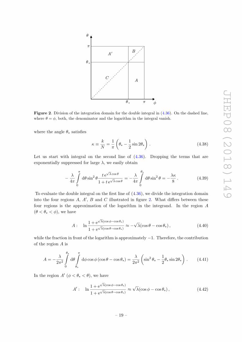
Figure 2. Division of the integration domain for the double integral in (4.36). On the dashed line,

where θ = φ, both, the denominator and the logarithm in the integral vanish.

where the angle θ∗ satisfies

κ ≡ k

N=

1

π

(θ∗ −

1

2sin 2θ∗

). (4.38)

Let us start with integral on the second line of (4.36). Dropping the terms that are

exponentially suppressed for large λ, we easily obtain

− λ

4π

π∫0

dθ sin2 θt e√λ cos θ

1 + t e√λ cos θ

= − λ

4π

θ∗∫0

dθ sin2 θ = −λκ8. (4.39)

To evaluate the double integral on the first line of (4.36), we divide the integration domain

into the four regions A, A′, B and C illustrated in figure 2. What differs between these

four regions is the approximation of the logarithm in the integrand. In the region A

(θ < θ∗ < φ), we have

A : ln1 + e

√λ(cosφ−cos θ∗)

1 + e√λ(cos θ−cos θ∗)

≈ −√λ(cos θ − cos θ∗) , (4.40)

while the fraction in front of the logarithm is approximately −1. Therefore, the contribution

of the region A is

A = − λ

2π2

θ∗∫0

dθ

π∫θ∗

dφ cosφ (cos θ − cos θ∗) =λ

2π2

(sin2 θ∗ −

1

2θ∗ sin 2θ∗

). (4.41)

In the region A′ (φ < θ∗ < θ), we have

A′ : ln1 + e

√λ(cosφ−cos θ∗)

1 + e√λ(cos θ−cos θ∗)

≈√λ(cosφ− cos θ∗) , (4.42)

– 19 –

JHEP08(2018)149

but the fraction in front of the logarithm is exponentially suppressed. Hence,

A′ = 0 . (4.43)

Next, look at region B, where θ > θ∗ and φ > θ∗. Here,

B : ln1 + e

√λ(cosφ−cos θ∗)

1 + e√λ(cos θ−cos θ∗)

≈ e√λ(cosφ−cos θ∗)

(1− e

√λ(cos θ−cosφ)

). (4.44)

The term in parentheses precisely cancels the denominator of the term in front of the

logarithm, and what remains of the integrand is again exponentially suppressed for large

λ. Thus,

B = 0 . (4.45)

In the remaining region C, where θ < θ∗ and φ < θ∗, we have

C : ln1 + e

√λ(cosφ−cos θ∗)

1 + e√λ(cos θ−cos θ∗)

≈√λ (cosφ− cos θ) . (4.46)

Therefore, we can write the contribution from the region C to the integral as

C = − λ

2π2

θ∗∫0

dθ

θ∗∫0

dφ cosφ (cosφ− cos θ)e√λ cos θ

e√λ cosφ− e

√λ cos θ

. (4.47)

Because the integration domain in (4.47) is symmetric with respect to φ and θ, we can

symmetrize the integrand and rewrite (4.47) as

C =λ

8π2

θ∗∫0

dθ

θ∗∫0

dφ

[(cosφ− cos θ)2 + (cos2 θ − cos2 φ)

e√λ cosφ + e

√λ cos θ

e√λ cosφ− e

√λ cos θ

]. (4.48)

The first term is readily integrated and yields

C1 =λ

8π2

θ∗∫0

dθ

θ∗∫0

dφ (cosφ− cos θ)2 =λ

8π2

(θ2∗ +

1

2θ∗ sin 2θ∗ − 2 sin2 θ∗

). (4.49)

In the second term in (4.48), we write cos2 θ − cos2 φ = sin2 φ − sin2 θ and realize that,

using the symmetry of the integrand and the integration domain, we can write

C2 =λ

4π2

θ∗∫0

dθ

θ∗∫0

dφ sin2 φe√λ cosφ + e

√λ cos θ

e√λ cosφ− e

√λ cos θ

. (4.50)

Here, the φ-integral must be interpreted as the principle value because of the pole for φ = θ,

whereas there was no pole with the symmetric integrand. However, after rewriting (4.50) as

C2 = −√λ

4π2

θ∗∫0

dθ

θ∗∫0

dφ sinφ∂φ

[ln∣∣∣e√λ(cos θ−cosφ)−1

∣∣∣+ ln∣∣∣e√λ cosφ− e

√λ cos θ

∣∣∣] , (4.51)

– 20 –

JHEP08(2018)149

the φ-integral is easily done using integration by parts, which also takes care of the principal

value. The result is

C2 =λ

8π2

(− sin2 θ∗ +

1

2θ∗ sin 2θ∗

). (4.52)

Summing the results (4.41), (4.43), (4.45), (4.49) and (4.52), we obtain the first line

of (4.36),

F1(t) =λ

8π2(θ2∗ − θ∗ sin 2θ∗ + sin2 θ∗

). (4.53)

This agrees with (3.53b) of [45].5

Finally, after adding (4.39) to (4.53) and using (4.38), we end up with the final result

for F1(t),

F1(t) =λ

8

[−κ(1− κ) +

1

π2sin4 θ∗

]. (4.54)

We note that (4.54) is symmetric under θ∗ → π − θ∗, which lets κ→ 1− κ. This reflects,

of course, the palindromic property of FA(t; I(g, g)). We also note that the first term

in brackets in (4.54) cancels against the exponential factor in (2.54), i.e., for the SU(N)

Wilson loop. This reproduces (3.56) of [45].

5 Conclusions

In this paper we tackled the problem of non-planar corrections to the expectation value of12 -BPS Wilson loops in N = 4 SYM with gauge group U(N) or SU(N). More precisely, we

extracted the leading and sub-leading behaviours in the 1/N expansion at fixed ’t Hooft

coupling λ of the Wilson loop generating function. Unlike previous works, which had

addressed this issue using loop equation techniques and topological recursion, our start-

ing point was the exact solution of the matrix model, which had been known for some

time. Our results for the 1/N term of the Wilson loop generating function agree with

previous calculations, but appear to be somewhat more explicit. We have provided both

sum and integral representations of the 1/N terms and have evaluated them explicitly in

the holographic large-λ regime, which allows for easier comparison with the holographic

dual picture. This term should match with the gravitational backreaction of the D-brane

on the gravity side. A particularly interesting observation is the connection between the

Wilson loop generating function and the finite-dimensional quantum system known as the

truncated harmonic oscillator. This system, which is familiar to the Quantum Optics

community, provides a description of the problem that seems to be more amenable to an

asymptotic 1/N expansion. En route, we obtained interesting mathematical relations and

sum rules involving the Hermite polynomials. It would be interesting to see these formulas,

which we proved in appendices D and E, in different applications.

One can envisage two main lines of generalization of the present work. First, it would

be interesting to extend the methods developed here to other representations of the gauge

group. A particularly interesting case is the totally symmetric representation Sk (see

also [47]), whose generating function is slightly more complicated than the antisymmetric

5The difference in the sign stems from the different definitions of F(t).

– 21 –

JHEP08(2018)149

one but still quite simple, so the problem seems tractable. Second, one may investigate how

the present approach extends to higher orders in 1/N . At first sight, there are a number of

technical obstacles that must be overcome, because order-1/N2 terms have been neglected

at many points of the calculation. So, the question whether our approach lends itself to

a systematic 1/N expansion is highly non-trivial. This problem is closely related to the

fact that the large, but finite-N matrix model solution differs in its analyticity properties

from the continuum limit. Moreover, corrections to the saddle point calculation of the

Wilson loop expectation values become relevant at order 1/N2. We leave these interesting

questions for the future.

Acknowledgments

A.C. and A.F. were supported by Fondecyt # 1160282. The research of W.M. was partly

supported by the I.N.F.N., research initiative STEFI.

A Some properties of the Hermite polynomials

In this appendix, we list a number of formulae regarding the (probabilists’) Hermite poly-

nomials, which are useful for the analysis in the main text. These relations can be found

in standard references [49, 52]. Sometimes a translation from the physicists’ version of the

polynomials is necessary. They are related by

Hen(x) = 2−n2 Hn(x/

√2) . (A.1)

The Hermite polynomials Hen(x) satisfy the differential equation

He′′n−xHe′n +nHen = 0 (A.2)

as well as the recurrence relations

He′n = nHen−1 , (A.3)

Hen+1 = xHen−nHen−1 . (A.4)

The generating function is

ext−12t2 =

∞∑n=0

tn

n!Hen(x) . (A.5)

Another useful property is the linearization formula

Hem(x) Hen(x) =m∑k=0

(m

k

)(n

k

)k! Hem+n−2k(x) . (A.6)

A main ingredient in our analysis is the location of the N roots of HeN for large N .

It can be obtained from the relation of HeN to the parabolic cylinder function

HeN (x) = ex2/4 U

(−N − 1

2, x

)(A.7)

– 22 –

JHEP08(2018)149

and the asymptotic expansion of the parabolic cylinder function

U

(−1

2µ2,√

2µt

)(A.8)

∼ 2g(µ)

(1− t2)1/4

[cosκ

∞∑s=0

(−1)su2s(t)

(1− t2)3sµ4s− sinκ

∞∑s=0

(−1)su2s+1(t)

(1− t2)3s+3/2µ4s+2

],

where

κ = µ2η − 1

4π , η =

1

2

(arccos t− t

√1− t2

), (A.9)

and us(t) are polynomials

u0 = 1, u1 =1

24t(t2 − 6) , · · · (A.10)

The function g(µ) is irrelevant for our purposes. Setting µ =√

2N + 1 and t = cos θ, these

relations imply that the N roots of HeN are given approximately by

ζi = 2

√N +

1

2cos θi , (A.11)

with (N +

1

2

)(θi −

1

2sin 2θi

)− 1

4π =

(i− 1

2

)π (i = 1, 2, . . . , N) . (A.12)

B Trace of normal ordered products

In this appendix, we calculate the trace of the normal ordered product ATmAn. First,

consider AT nAn. Using the definition of the number operator (2.28) and the commuta-

tors (2.29), we get

AT nAn = AT n−1NAn−1 = AT n−1An−1(N − n+ 1) = (N − n+ 1)n , (B.1)

where we have iterated the first two steps to arive at the final expression. (a)n = Γ(a +

n)/Γ(a) denotes the Pochhammer symbol. This allows us to write immediately

ATmAn =

{ATm−n(N − n+ 1)n for m ≥ n,

(N −m+ 1)mAn−m for m < n.

(B.2)

Because N is diagonal and any power of A is off-diagonal, the trace of this quantity is

non-zero only, if m = n,

Tr(ATmAn

)= δmn Tr(N − n+ 1)n . (B.3)

The trace in (B.3) can be calculated starting with the expansion of the Pochhammer symbol

in terms of Stirling numbers [52]. This gives

Tr(N − n+ 1)n =n∑l=0

s(n, l) TrN l =n∑l=0

s(n, l)N−1∑k=0

kl

=n∑l=1

s(n, l)l∑

j=0

j!

(N

j + 1

)S(l, j) , (B.4)

– 23 –

JHEP08(2018)149

where S(l, j) denote the Stirling numbers of the second kind. After rearranging the sum

and using the properties of the Stirling numbers, (B.4) becomes

Tr(N − n+ 1)n = n!

(N

n+ 1

)=

(N − n)n+1

n+ 1. (B.5)

Finally, expressing the Pochhammer symbol in terms of Stirling numbers of the first kind

yields an expansion in 1/N ,

1

Nn+1Tr(N − n+ 1)n =

1

n+ 1

n∑l=0

s(n+ 1, n+ 1− l)N−l . (B.6)

C Conversion of the sum over the roots of HeN to an integral

Consider a sum of the form

1

N

N∑i=1

f(θi) , (C.1)

where θi are defined in (A.11) in terms of the zeros of the Hermite polynomial HeN (ζ). In

the large N limit, it is justified to convert such a sum into an integral. Here we describe

here how to do it correctly to order 1/N .

We start by setting x = i − 12 and use the Euler-Maclaurin formula in mid-point

form [53]. The mid-point form has the advantages that the integration domain lies man-

ifestly symmetric within the inveral (0, N) and that the boundary terms in the Euler-

Maclaurin formula contain only derivatives of the integrand. The latter turn out to con-

tribute at least of order 1/N2 and are, therefore, irrelevant for our purposes. Hence, we have

1

N

N∑i=1

f(θi) =1

N

N∫0

dxf(θx+1/2) +O(

1

N2

)

=2

π

(1 +

1

2N

) π−θ1/2∫θ1/2

dθ sin2 θf(θ) +O(

1

N2

). (C.2)

In the second equality, we have changed the integration variable using (A.11). The angle

θ1/2, which marks the tiny edges missing from the interval (0, π), also follows from (A.11),(N +

1

2

)(θ1/2 −

1

2sin 2θ1/2

)=

1

4π ⇒ θ31/2 ≈

3π

8N. (C.3)

Therefore, (C.2) becomes

1

N

N∑i=1

f(θi) =2

π

(1 +

1

2N

) π∫0

dθ sin2 θf(θ)− 1

4N[f(0) + f(π)] +O

(1

N2

). (C.4)

To obtain the second term on the right hand side we have assumed that the function f is

regular at 0 and π.

– 24 –

JHEP08(2018)149

Let us check the formula (C.4) by calculating the trace of the matrix I(g, g) in the posi-

tion basis (4.18) and compare the result with the exact expression, which can be calculated

in the number basis as follows,6

1

NTr(

egA†

egA)

=N−1∑k,l=0

gk+l

k!l!

1

NTr(A†kAl

)

=N−1∑k=0

g2k

(k!)21

NTr(N − k + 1)k

=

N−1∑k=0

g2kNk

k!(k + 1)!

k∑l=0

s(k + 1, k + 1− l)N−l

=

(1− λ

8N

)2√λ

I1(√λ) +O

(1

N2

). (C.5)

In the position basis, we have from (4.18) and (C.4)

1

NTr I(g, g) =

2

π

(1 +

1

2N

) π∫0

dθ sin2 θ e2g

√N+ 1

2cos θ− 1

2g2

+1

N

∞∑r,s=1

Ir+s(√λ)

2

π

π∫0

dθ sin(rθ) sin(sθ)− 1

2Ncosh

√λ

=

(1 +

1

2N

)e−

λ8N

2√λ√

1 + 12N

I1

(√λ

√1 +

1

2N

)

+1

N

∞∑r=1

I2r(√λ)− 1

2Ncosh

√λ

=2√λ

I1(√λ) e−

λ8N +

1

N

[1

2I0(√λ) +

∞∑r=1

I2r(√λ)− 1

2cosh

√λ

]

=2√λ

I1(√λ) e−

λ8N . (C.6)

We especially point out the presence of the last term on the second line, which comes

from the edge terms of (C.4) and is crucial for cancelling other 1/N contributions. The

bracket on the penultimate line vanishes by means of a well-known summation formula of

the modified Bessel functions [52]. In these expressions, we have dropped all contributions

of order 1/N2. Obviously (C.6) agrees with (C.5) to order 1/N .

D Proof of (4.16)

In this appendix, we provide a proof of the asymptotic formula

HeN−s(ζ)

HeN+1(ζ)∼ −(N − s)!

N !N

s−12 Us−1(cos θ) , (D.1)

6This calculation appeared already in section 3 between (3.2) and (3.3) and makes use of the calculation

in appendix B.

– 25 –

JHEP08(2018)149

which is (4.16) in the main text. This formula holds for s � N , and ζ ∼ 2√N cos θ is a

root of HeN .

The proof is done by induction using the recursion formula for the Hermite polynomi-

als (A.4). First, consider s = 1 and s = 2. Because ζ is a root of HeN , we have

HeN−1(ζ) = − 1

NHeN+1(ζ) , (D.2)

HeN−2(ζ) =1

N − 1ζ HeN−1(ζ) = − 1

N(N − 1)N

12 2 cos θHeN+1(ζ) , (D.3)

so (D.1) obviously holds for s = 1 and s = 2. Now, assume that (D.1) holds for HeN−s+1.

Then, from the recursion formula (A.4) we get

HeN−s(ζ) =1

N − s+ 1[ζ HeN−s+1(ζ)−HeN−s+2(ζ)] ,

HeN−s(ζ)

HeN−1(ζ)= − 1

N − s+ 1

[2√N cos θ

(N − s+ 1)!

N !N

s−22 Us−2(cos θ)

−(N − s+ 2)!

N !N

s−32 Us−3(cos θ)

]= −(N − s)!

N !N

s−12

[2 cos θUs−2(cos θ)− N − s+ 2

NUs−3(cos θ)

]∼ −(N − s)!

N !N

s−12 Us−1(cos θ) ,

where we have dropped the term s of order 1/N in front of Us−3(cos θ) and used the

recursion relation for the Chebychev polynomials [49] in the last step.

E Proof of (4.29)

In this appendix, we shall prove the remarkable summation formula

v∑r=1

∞∑t1=1

· · ·∞∑

ta−1=1

Iv−r+t1(z) It2−t1(z) · · · Ir−ta−1(z) =v

aIv(az) , a = 2, 3, . . . . (E.1)

For a = 2, we have established the result in (4.28). Our starting point is the generating

function of the modified Bessel functions (4.19),

ez cos θ = I0(z) + 2

∞∑k=1

Ik(z) cos(kθ) . (E.2)

Differentiating it with respect to θ shows that

z

2sin θ eaz cos θ =

∞∑k=1

k Ik(az)

asin(kθ) . (E.3)

Therefore, we can prove (E.1) by showing that

∞∑v=1

Sa(v; z) sin(vθ) =z

2sin θ eaz cos θ , (E.4)

– 26 –

JHEP08(2018)149

where Sa(v; z) is, as defined in the main text, the left hand side of (E.1). Since S2(v; z) is

known from (4.28), (E.4) trivially holds for a = 2 by virtue of (E.3).

The left hand side of (E.4) is explicitly

∞∑v=1

Sa(v; z) sin(vθ) =∞∑v=1

sin(vθ)v∑r=1

∞∑t1=1

· · ·∞∑

ta−1=1

Iv−r+t1(z) It2−t1(z) · · · Ir−ta−1(z) .

(E.5)

We rearrange the sums over v and r by introducing s = v − r and ta = r, such that

∞∑v=1

Sa(v; z) sin(vθ) =

∞∑s=0

∞∑ta=1

· · ·∞∑t1=1

sin[(s+ ta)θ] Ita−ta−1(z) · · · It2−t1(z) Is+t1(z) . (E.6)

Now, we can extend the summation over ta to all integers without changing the value of

the sum. The reason for this is that

∞∑s=0

∞∑r=0

sin[(s− r)θ]Mrs = 0 , (E.7)

if Mrs is symmetric, by the antisymmetry of the sine. It is easy to see that this is the case

for the matrix involving the rest of the t-summations and the modified Bessel functions

in (E.6). Therefore,

∞∑v=1

Sa(v; z) sin(vθ) =∞∑s=0

∞∑ta=−∞

∞∑ta−1=1

· · ·∞∑t1=1

sin[(s+ ta)θ] Ita−ta−1(z) · · · It2−t1(z) Is+t1(z)

=

∞∑s=0

∞∑ta−1=1

· · ·∞∑t1=1

∞∑ta=−∞

{sin[(s+ ta−1)θ] cos(taθ) + cos[(s+ ta−1)θ] sin(taθ)}

× Ita(z) Ita−1−ta−2(z) · · · It2−t1(z) Is+t1(z)

= ez cos θ∞∑v=1

Sa−1(v; z) sin(vθ) . (E.8)

In the step to the last line, we have carried out the sum over ta using (E.2) and used the

fact that the sum of sin(taθ) Ita(z) vanishes. Continuing recursively, we obtain

∞∑v=1

Sa(v; z) sin(vθ) = e(a−2)z cos θ∞∑v=1

S2(v; z) sin(vθ) =z

2sin θ eaz cos θ , (E.9)

knowing that (E.4) is true for a = 2. Thus, we have proven (E.4) for all a ≥ 2, which

implies (E.1).

Open Access. This article is distributed under the terms of the Creative Commons

Attribution License (CC-BY 4.0), which permits any use, distribution and reproduction in

any medium, provided the original author(s) and source are credited.

– 27 –

JHEP08(2018)149

References

[1] J.M. Maldacena, Wilson loops in large N field theories, Phys. Rev. Lett. 80 (1998) 4859

[hep-th/9803002] [INSPIRE].

[2] S.-J. Rey and J.-T. Yee, Macroscopic strings as heavy quarks in large N gauge theory and

anti-de Sitter supergravity, Eur. Phys. J. C 22 (2001) 379 [hep-th/9803001] [INSPIRE].

[3] J.K. Erickson, G.W. Semenoff and K. Zarembo, Wilson loops in N = 4 supersymmetric

Yang-Mills theory, Nucl. Phys. B 582 (2000) 155 [hep-th/0003055] [INSPIRE].

[4] N. Drukker and D.J. Gross, An exact prediction of N = 4 SUSYM theory for string theory,

J. Math. Phys. 42 (2001) 2896 [hep-th/0010274] [INSPIRE].

[5] V. Pestun, Localization of gauge theory on a four-sphere and supersymmetric Wilson loops,

Commun. Math. Phys. 313 (2012) 71 [arXiv:0712.2824] [INSPIRE].

[6] K. Zarembo, Supersymmetric Wilson loops, Nucl. Phys. B 643 (2002) 157 [hep-th/0205160]

[INSPIRE].

[7] N. Drukker, 1/4 BPS circular loops, unstable world-sheet instantons and the matrix model,

JHEP 09 (2006) 004 [hep-th/0605151] [INSPIRE].

[8] N. Drukker, S. Giombi, R. Ricci and D. Trancanelli, Wilson loops: from four-dimensional

SYM to two-dimensional YM, Phys. Rev. D 77 (2008) 047901 [arXiv:0707.2699] [INSPIRE].

[9] N. Drukker, S. Giombi, R. Ricci and D. Trancanelli, More supersymmetric Wilson loops,

Phys. Rev. D 76 (2007) 107703 [arXiv:0704.2237] [INSPIRE].

[10] N. Drukker, S. Giombi, R. Ricci and D. Trancanelli, Supersymmetric Wilson loops on S3,

JHEP 05 (2008) 017 [arXiv:0711.3226] [INSPIRE].

[11] G.W. Semenoff and D. Young, Exact 1/4 BPS loop: chiral primary correlator, Phys. Lett. B

643 (2006) 195 [hep-th/0609158] [INSPIRE].

[12] S. Giombi, R. Ricci and D. Trancanelli, Operator product expansion of higher rank Wilson

loops from D-branes and matrix models, JHEP 10 (2006) 045 [hep-th/0608077] [INSPIRE].

[13] J. Gomis, S. Matsuura, T. Okuda and D. Trancanelli, Wilson loop correlators at strong

coupling: from matrices to bubbling geometries, JHEP 08 (2008) 068 [arXiv:0807.3330]

[INSPIRE].

[14] S. Giombi and V. Pestun, Correlators of local operators and 1/8 BPS Wilson loops on S2

from 2d YM and matrix models, JHEP 10 (2010) 033 [arXiv:0906.1572] [INSPIRE].

[15] A. Bassetto, L. Griguolo, F. Pucci, D. Seminara, S. Thambyahpillai and D. Young,

Correlators of supersymmetric Wilson-loops, protected operators and matrix models in N = 4

SYM, JHEP 08 (2009) 061 [arXiv:0905.1943] [INSPIRE].

[16] A. Bassetto, L. Griguolo, F. Pucci, D. Seminara, S. Thambyahpillai and D. Young,

Correlators of supersymmetric Wilson loops at weak and strong coupling, JHEP 03 (2010)

038 [arXiv:0912.5440] [INSPIRE].

[17] S. Giombi and V. Pestun, Correlators of Wilson loops and local operators from multi-matrix

models and strings in AdS, JHEP 01 (2013) 101 [arXiv:1207.7083] [INSPIRE].

[18] M. Bonini, L. Griguolo and M. Preti, Correlators of chiral primaries and 1/8 BPS Wilson

loops from perturbation theory, JHEP 09 (2014) 083 [arXiv:1405.2895] [INSPIRE].

– 28 –

JHEP08(2018)149

[19] J. Aguilera-Damia, D.H. Correa, F. Fucito, V.I. Giraldo-Rivera, J.F. Morales and L.A.

Pando Zayas, Strings in bubbling geometries and dual Wilson loop correlators, JHEP 12

(2017) 109 [arXiv:1709.03569] [INSPIRE].

[20] B. Fraser and S.P. Kumar, Large rank Wilson loops in N = 2 superconformal QCD at strong

coupling, JHEP 03 (2012) 077 [arXiv:1112.5182] [INSPIRE].

[21] J.G. Russo and K. Zarembo, Large N limit of N = 2 SU(N) gauge theories from localization,

JHEP 10 (2012) 082 [arXiv:1207.3806] [INSPIRE].

[22] J.G. Russo and K. Zarembo, Localization at large N , in Proceedings, 100th anniversary of the

birth of I.Ya. Pomeranchuk (Pomeranchuk 100), Moscow, Russia, 5–6 June 2013, World

Scientific, Singapore, (2014), pg. 287 [arXiv:1312.1214] [INSPIRE].

[23] B. Fraser, Higher rank Wilson loops in the N = 2 SU(N)× SU(N) conformal quiver, J.

Phys. A 49 (2016) 02LT03 [arXiv:1503.05634] [INSPIRE].

[24] J.T. Liu, L.A. Pando Zayas and S. Zhou, Comments on higher rank Wilson loops in N = 2∗,

JHEP 01 (2018) 047 [arXiv:1708.06288] [INSPIRE].

[25] J.G. Russo and K. Zarembo, Wilson loops in antisymmetric representations from localization

in supersymmetric gauge theories, World Scientific, Singapore, (2018), pg. 419

[arXiv:1712.07186] [INSPIRE].

[26] M. Billo, F. Galvagno, P. Gregori and A. Lerda, Correlators between Wilson loop and chiral

operators in N = 2 conformal gauge theories, JHEP 03 (2018) 193 [arXiv:1802.09813]

[INSPIRE].

[27] J. Gomis and F. Passerini, Holographic Wilson loops, JHEP 08 (2006) 074 [hep-th/0604007]

[INSPIRE].

[28] S. Yamaguchi, Wilson loops of anti-symmetric representation and D5-branes, JHEP 05

(2006) 037 [hep-th/0603208] [INSPIRE].

[29] S. Yamaguchi, Bubbling geometries for half BPS Wilson lines, Int. J. Mod. Phys. A 22

(2007) 1353 [hep-th/0601089] [INSPIRE].

[30] O. Lunin, On gravitational description of Wilson lines, JHEP 06 (2006) 026

[hep-th/0604133] [INSPIRE].

[31] E. D’Hoker, J. Estes and M. Gutperle, Gravity duals of half-BPS Wilson loops, JHEP 06

(2007) 063 [arXiv:0705.1004] [INSPIRE].

[32] T. Okuda and D. Trancanelli, Spectral curves, emergent geometry and bubbling solutions for

Wilson loops, JHEP 09 (2008) 050 [arXiv:0806.4191] [INSPIRE].

[33] S.A. Hartnoll and S.P. Kumar, Higher rank Wilson loops from a matrix model, JHEP 08

(2006) 026 [hep-th/0605027] [INSPIRE].

[34] S. Forste, D. Ghoshal and S. Theisen, Stringy corrections to the Wilson loop in N = 4 super

Yang-Mills theory, JHEP 08 (1999) 013 [hep-th/9903042] [INSPIRE].

[35] N. Drukker, D.J. Gross and A.A. Tseytlin, Green-Schwarz string in AdS5 × S5: semiclassical

partition function, JHEP 04 (2000) 021 [hep-th/0001204] [INSPIRE].

[36] M. Kruczenski and A. Tirziu, Matching the circular Wilson loop with dual open string

solution at 1-loop in strong coupling, JHEP 05 (2008) 064 [arXiv:0803.0315] [INSPIRE].

[37] A. Faraggi and L.A. Pando Zayas, The spectrum of excitations of holographic Wilson loops,

JHEP 05 (2011) 018 [arXiv:1101.5145] [INSPIRE].

– 29 –

JHEP08(2018)149

[38] A. Faraggi, W. Muck and L.A. Pando Zayas, One-loop effective action of the holographic

antisymmetric Wilson loop, Phys. Rev. D 85 (2012) 106015 [arXiv:1112.5028] [INSPIRE].

[39] A. Faraggi, J.T. Liu, L.A. Pando Zayas and G. Zhang, One-loop structure of higher rank

Wilson loops in AdS/CFT, Phys. Lett. B 740 (2015) 218 [arXiv:1409.3187] [INSPIRE].

[40] V. Forini, V. Giangreco M. Puletti, L. Griguolo, D. Seminara and E. Vescovi, Precision

calculation of 1/4-BPS Wilson loops in AdS5 × S5, JHEP 02 (2016) 105

[arXiv:1512.00841] [INSPIRE].

[41] A. Faraggi, L.A. Pando Zayas, G.A. Silva and D. Trancanelli, Toward precision holography

with supersymmetric Wilson loops, JHEP 04 (2016) 053 [arXiv:1601.04708] [INSPIRE].

[42] V. Forini, A.A. Tseytlin and E. Vescovi, Perturbative computation of string one-loop

corrections to Wilson loop minimal surfaces in AdS5 × S5, JHEP 03 (2017) 003

[arXiv:1702.02164] [INSPIRE].

[43] J. Aguilera-Damia, A. Faraggi, L.A. Pando Zayas, V. Rathee and G.A. Silva, Toward

precision holography in type IIA with Wilson loops, JHEP 08 (2018) 044

[arXiv:1805.00859] [INSPIRE].

[44] J. Aguilera-Damia, A. Faraggi, L.A. Pando Zayas, V. Rathee and G.A. Silva, Zeta-function

regularization of holographic Wilson loops, Phys. Rev. D 98 (2018) 046011

[arXiv:1802.03016] [INSPIRE].

[45] J. Gordon, Antisymmetric Wilson loops in N = 4 SYM beyond the planar limit, JHEP 01

(2018) 107 [arXiv:1708.05778] [INSPIRE].

[46] K. Okuyama, Phase transition of anti-symmetric Wilson loops in N = 4 SYM, JHEP 12

(2017) 125 [arXiv:1709.04166] [INSPIRE].

[47] X. Chen-Lin, Symmetric Wilson loops beyond leading order, SciPost Phys. 1 (2016) 013

[arXiv:1610.02914] [INSPIRE].

[48] B. Fiol and G. Torrents, Exact results for Wilson loops in arbitrary representations, JHEP

01 (2014) 020 [arXiv:1311.2058] [INSPIRE].

[49] I.S. Gradshteyn and I.M. Ryzhik, Table of integrals, series and products, 5th edition,

Academic Press, New York, U.S.A., (1994).

[50] E. Pisanty and E. Nahmad-Achar, On the spectrum of field quadratures for a finite number

of photons, J. Phys. A 45 (2012) 395303 [arXiv:1109.5724].

[51] K.E. Cahill and R.J. Glauber, Ordered expansions in boson amplitude operators, Phys. Rev.

177 (1969) 1857 [INSPIRE].

[52] NIST Digital Library of Mathematical Functions, release 1.0.16, http://dlmf.nist.gov/, 18

September 2017.

[53] D. Sarafyan, L. Derr and C. Outlaw, Generalizations of the Euler-Maclaurin formula, J.

Math. Anal. Appl. 67 (1979) 542.

– 30 –