Anthropogenic impacts on high-latitude ecosystems: Shrubs will grow. Will nitrogen flow?

A DISSERTATION SUBMITTED TO THE FACULTY OF

UNIVERSITY OF MINNESOTA BY

Daniel E. Ackerman

IN PARTIAL FULFILLMENT OF THE REQUIREMENTS FOR THE DEGREE OF

DOCTOR OF PHILOSOPHY

College of Biological Sciences

Dr. Jacques Finlay, Adviser Dr. Daniel Griffin, Co-Adviser

May 2019

i

Acknowledgements

This dissertation is not an individual accomplishment. I am grateful to many

people, both within the University of Minnesota and beyond, who have supported me

throughout my PhD program.

I thank my co-advisers, Jacques Finlay and Dan Griffin, for indulging my wildly

disparate interests in high-latitude ecology and for pushing me to develop as a scientist,

writer, presenter, and person. Jacques’ passion for and deep knowledge of biogeogemical

cycling, from the arctic tundra to his St. Paul backyard, were both instructional and

inspirational. Dan taught me how to read climate history in a tree trunk, and kept me from

going crazy and cross-eyed in the midst of measuring 19,624 microscopic shrub rings.

I also thank my committee members, Sarah Hobbie and Jim Cotner, for providing

invaluable feedback on my scientific thinking and writing. The rest of the EEB

department, especially the 2014 cohort and the members of the Finlay lab, have helped

me grow both intellectually and socially during my time here. I will miss playing in the

weekly EEB pick-up basketball game.

Many brilliant and kind scientists outside the EEB department also served as

informal mentors. Their wisdom improved the quality of my work and often enabled

projects I was not equipped to complete on my own. In particular, I thank Gus Shaver,

Ken Tape, Heidi Golden, Ben Jones, Breck Bowden, Laura Gough, Isla Myers-Smith,

Scott St. George, Ingibjörg Svala Jónsdóttir, Dylan Millet, and Xin Chen.

I have many institutions to thank for vital funding and logistical support for my

research: National Science Foundation, Bell Museum of Natural History, Explorers Club,

ii

UMN EEB Department, Marine Biological Laboratory, Toolik Field Station, US

Geological Survey, and the Long Term Ecological Research network.

In the past five years, a number of housemates have put up with my (often

strange) schedule, respected my need for quiet when I was cramming to meet a deadline,

and supported me through times of stress. These wonderful beings include Karl Snyder,

Justin Carlson, Robert Hest, Emily Houser, and Wizard the cat.

My parents, Jerry Ackerman and Beth Goldbaum, provided me guidance, support,

and love, long before I knew what an ecologist was. Thank you for encouraging me to

find and follow my passion. My earliest explorations of nature happened under the wing

of my big sister, Rachel Ackerman Morrow, among the trees and dirt of our family’s

backyard, which seemed a vast wilderness to small children. Now from the verdant

mountains of Kauai, she continues to inspire me to enjoy nature every day.

My wife, Sarah Nalven, has provided more love and support than I could ever

express here. Thank you.

iii

Table of contents

List of Tables…………………………………………………………………………..…iv

List of Figures……………………………………………………………………………..v

Introduction……………………………………………………………………………… .1

Chapter 1: Arctic shrub growth trajectories differ across soil moisture levels…………....9

Chapter 2: Uniform shrub growth response to June temperature across the North Slope of Alaska…………………………………………………………………......…35

Chapter 3: Global estimates of inorganic nitrogen deposition across four decades……..57

Chapter 4: Temperature controls nitrogen retention in circumarctic watersheds….…….74

Bibliography……………………………………………………………………………..96

Appendix 1: Chapter 1 Supplemental Material……………………………………..….114

Appendix 2: Chapter 3 Supplemental Material……………………………………..….120

Appendix 3: Chapter 4 Supplemental Material………………………………………...126

iv

List of Tables

1.1. Site characteristics (upland versus riparian)……………………………………..….32

1.2. Chronology statistics………………………………………………………………...33

1.3. Summary of climate sensitivity and climate-growth analysis…………………...….34

2.1. Characteristics of four glacial landscapes samples across the North Slope of Alaska………………………………………………………………………………...….54

2.2. Fixed effect coefficient estimates for the parsimonious and full mixed models predicting Salix pulchra ring width…………………………………………………..….55

2.3. Shrub characteristics from upland and riparian populations………………………..56

4.1. Fixed effects coefficient estimates for the full and parsimonious proportional nitrogen retention models…………………………………………………………….….94

4.2. Fixed effects coefficient estimates for the absolute nitrogen deposition model…….95

v

List of Figures

1.1. Diminishing growth returns to increasing temperature……………………………..25

1.2. Example of Salix pulchra radius wit growth increments from 1964 to 2014…...….26

1.3. First-order linear relationship between ring width index and mean June temperature……………………………………………………………………………....27

1.4. Moving window analysis for upland and riparian sites………………………….….28

1.5. Scatterplots and time series relating ring width index and mean June temperature……………………………………………………………………………....29

1.6. Aboveground Salix pulchra biomass for present-day temperature regime and a two-degree (C) increase in mean June temperature………………………………………..…30

1.7. Overlay of best-fit models relating ring width index to mean June temperature…....31

2.1. Landscape age in the circumpolar arctic tundra………………………………….....50

2.2. Z-scores of median ring width index correlate with mean June temperature…...…..51

2.3. Mean June temperature correlates positively with ring width index……………..…52

2.4. Stem length correlates with mean ring width………………………………….........53

3.1. Evaluation of simulated spatial and temporal trends in inorganic nitrogen deposition………………………………………………………………………………..70

3.2. Mean annual inorganic nitrogen deposition as simulated for the past four decades……………………………………………………………………………….….71

3.3. Mean annual rate of change in simulated total inorganic nitrogen deposition between 1984 and 2016………………………………………………………………………...…72

3.4. Change in percent of inorganic nitrogen deposited as chemically reduced molecules from 1984 to 2016…………………………………………………………………….…73

4.1. Conceptual model of nitrogen transport and watershed retention…………………..89

4.2. Circumpolar stream and river sites with total annual nitrogen export measurements………………………………………………………………………..…..90

4.3. Proportional nitrogen retention was positively related to mean annual temperature for 98 watersheds across the circumpolar north……………………………………………91

4.4. Absolute mass of nitrogen retained was positively related to both atmospheric nitrogen deposition and mean annual temperature……………………………………....92

4.5. Annual nitrogen export via streams and rivers and watershed retention versus atmospheric deposition for 98 high-latitude watersheds…………………………….....93

1

Introduction

Human activity is a dominant force shaping the structure and function of Earth’s

ecosystems. Some of these impacts are direct and local: phosphorus-rich runoff from

urban landscapes causes excessive siltation, eutrophication, and biodiversity reduction in

waterways (Carpenter et al. 1998, Paul and Meyer 2001). Other impacts are indirect and

regional: ozone precursors released from vehicles in cities can travel downwind and form

ozone harmful to plants, animals, and people (Keiser et al. 2018). Still other

anthropogenic impacts have profound consequences worldwide, namely fossil fuel

combustion and the release of carbon dioxide, a greenhouse gas, into a globally-mixed

troposphere (Hayhoe et al. 2018).

Due to these teleconnections between human action and environmental impact,

ecosystems that appear remote from direct human modification are still molded by our

societal behavior. This is particularly true of northern high-latitude ecosystems, including

arctic tundra and boreal forest. Cold temperatures and nitrogen limitation of terrestrial

primary productivity make these biomes highly sensitive to warming and atmospheric

nitrogen deposition, two widespread impacts of fossil fuel combustion (Elser et al. 2007,

LeBauer and Treseder et al. 2008, Elmendorf et al. 2012a, Shaver et al. 2014).

Background on anthropogenic changes

This dissertation will examine high-latitude ecosystem responses to warming and

atmospheric nitrogen deposition. The following two subsections provides background on

these topics.

High latitude warming

2

The arctic tundra biome is warming twice as fast as the global average (Cohen et al.

2012). Paleoclimate proxies indicate that such polar amplification has been a reliable

response to rising temperatures for at least the last three million years of Earth’s climate

history (Miller et al. 2010). This phenomenon is largely caused by the ice-albedo

feedback, but other contributing factors include changes in oceanic and atmospheric heat

transfer, increased near-surface cloud cover and atmospheric water vapor, and soot

deposition (Serreze and Barry, 2011).

A rapidly warming arctic is a source of considerable uncertainty in climate

projections due to poorly constrained biophysical carbon cycle feedbacks. Soils of high-

latitude permafrost regions contain nearly 1,700 Pg of organic carbon, equivalent to

roughly double the global atmospheric carbon pool (Tarnocai et al. 2009). As permafrost

thaws, much of the permafrost organic carbon pool will be metabolized by microbes into

atmospheric methane (in wet environments) or carbon dioxide (in dry environments). The

magnitude and rate of change in land-to-atmosphere carbon fluxes from permafrost

remains a topic of vigorous debate—“Methane bomb” media headlines may be too

sensationalized (Petrenko et al. 2017), but a gradual and sustained carbon release (Schuur

et al. 2015) may be too optimistic.

In addition to permafrost carbon feedbacks, high-latitude vegetation changes

could trigger both positive and negative feedbacks to climate change. For example, the

expansion of woody deciduous shrubs in circumarctic tundra could accelerate climate

change through positive feedback mechanisms including albedo reduction, competitive

exclusion of permafrost-insulating Sphagnum spp., and the capture of deep snowpacks

that increase microbial respiration through elevated winter soil temperatures (Sturm et al.

3

2001, Cornelissen et al. 2001, Blok et al. 2011a, Chapin et al. 2005, Lawrence and

Swenson 2011). Alternatively, shrub expansion could mitigate climate change through

negative feedback mechanisms including increased primary productivity, woody stem

production, recalcitrant litter chemistry, and shading of carbon-rich permafrost soils in

summer (Shaver 1986, Sweet et al. 2015, Cornelissen et al. 2007, Blok et al. 2011a,

Nauta et al. 2015). While the balance of such positive and negative feedbacks remains an

area of active research, integrating these feedbacks into earth systems models will

ultimately require accurate predictions of shrub expansion rates across space. In other

words, shrub expansion has not and will not proceed at a uniform pace throughout the

tundra. Chapters 1 and 2 of this dissertation seek to determine which factors underlie the

variable rates of shrub expansion across environmental gradients in arctic tundra.

Nitrogen deposition

Humans have doubled the amount of bio-reactive nitrogen entering the biosphere in the

industrial era through fertilization, biomass and fossil fuel combustion, and volatilization

from agricultural materials such as manure (Galloway et al. 2004, Galloway et al. 2008).

Despite major improvements in agricultural production, the rapid increase in nitrogen

availability has wide-ranging consequences for human health, ecosystem function, and

community structure. For example, nitrate-loading in groundwater aquifers in highly

fertilized agricultural regions is linked to methemoglobinemia (blue-baby syndrome) and

is believed to be a risk factor for certain cancers and birth defects (Spalding and Exner

1993, Weyer et al. 2008, Brender et al. 2013). In nitrogen-limited terrestrial ecosystems,

increased availability boosts primary productivity, often causing community shifts toward

dominance by species with low nitrogen-use efficiencies (Stevens et al. 2004, Clark and

4

Tilman 2008). Elevated delivery of nitrogen to nitrogen-limited (or nitrogen and

phosphorus co-limited) freshwater and marine ecosystems can fuel algae blooms that

harm plants and animals through light attenuation and oxygen depletion (Howarth and

Marino 2006, Conley et al. 2009, Finlay et al. 2013). There is an urgent need to assess

the capability of global ecosystems to buffer this nitrogen cycle intensification through

nitrogen uptake by organisms and denitrification.

Understanding ecosystem response to elevated nitrogen deposition is particularly

crucial at high latitudes, where nitrogen limitation is widespread across the boreal forest

and arctic tundra biomes (Elser et al. 2007, LeBauer and Treseder et al. 2008, Shaver et

al. 2014). Primary productivity and community composition in these systems is highly

sensitive to changes in nitrogen availability (Wookey et al. 1994, Chapin and Shaver

1996, Van Wijk et al. 2004, Hobbie et al. 2005). Therefore, future changes in

atmospheric nitrogen deposition, which tend to be regional in scale, could restructure

ecosystem function and community composition in some areas.

Strategies for studying ecosystem response to anthropogenic changes

The following two subsections review methods used to research ecosystem impacts of

warming and elevated nitrogen availability. The four chapters of this dissertation will

both incorporate and build upon some of these methods.

Shrub expansion

Researchers have employed a variety of experimental and observational techniques to

determine environmental drivers of shrub expansion in arctic tundra. Early factorial

experiments crossing nutrient addition, warming, and insolation reduction suggested that

nitrogen availability was the limiting factor to primary productivity in arctic tundra

5

(Wookey et al. 1994, Chapin and Shaver 1996). This limitation was believed to be caused

by low mineralization rates, despite large pools of soil organic nitrogen (Shaver and

Jonasson 1999). Nitrogen addition appeared to lend a competitive advantage to species

with low nitrogen-use efficiencies, such as deciduous shrubs (Bret-Harte et al. 2001).

Subsequent experiments throughout the arctic tundra have further supported this idea

(DeMarco et al. 2014). Additional evidence for tundra shrub expansion has been

provided through observational techniques including repeat photography and remote

sensing (Tape et al. 2006, Myers-Smith et al. 2011).

Dendrochronology, the study of annual growth of woody plants, is becoming an

increasingly popular observational approach for studying shrub response to climate

(Myers-Smith et al. 2015a). This technique can provide a centennial-scale growth record,

longer than any experimental manipulation or remote sensing measure in the arctic

(Weijers et al. 2010). Further, the chronology of annual ring widths or other anatomical

measurements is a vast improvement in temporal resolution over previously used

methods such as repeat photography (Tape et al. 2006). Dendrochronological studies

have revealed historic relationships between climate and shrub growth in a wide range of

shrub growth forms, from prostrate evergreen species, e.g. Cassiope tetragona, to erect

deciduous species, e.g. Alnus viridis, Salix pulchra, and Betula nana (Weijers et al. 2010,

Blok et al. 2011a, Tape et al. 2012).

While dendrochronology appears to be a promising method, challenges remain in

connecting climate and environmental variability to individual plant response. The

traditional way to analyze arctic shrub dendrochronology data is to construct a site-based,

annually-resolved chronology of the central tendency of growth (usually a mean or

6

median of individually detrended ring-width indices) for the sample site (Cook and

Pederson 2011). This approach yields a uniform growth signal shared among shrubs at a

site, but it discards information related to the variability in climate response among

individuals (Galván et al. 2014, Young et al. 2016). An overarching goal of chapters 1

and 2 of this dissertation is to compare microsites and use individual-based statistical

modeling frameworks to examine variability in the climate-growth relationship among

individual shrubs on the North Slope of Alaska.

Nitrogen cycling

Long-term measurements of atmospheric nitrogen deposition are available for some high

latitude sites, but deposition estimates remain poorly constrained for many regions of the

vast arctic tundra and boreal forest biomes (Vet et al. 2014). Spatial models of nitrogen

deposition tend to have low, centennial-scale temporal resolution (Galloway et al. 2004).

Such models are insufficient for understanding nitrogen dynamics on shorter timescales,

because interannual nitrogen deposition in remote areas of the arctic can vary widely

based on stochastic weather and atmospheric transport events (Choudhary et al. 2016).

This uncertainty complicates the construction of nitrogen budgets for high-latitude

watersheds. Chapter 3 attempts to resolve this uncertainty by creating a spatially explicit

model of global nitrogen deposition with annual- to decadal-scale temporal resolution.

Little is known about the drivers of variability in nitrogen retention among

watersheds at a circumpolar scale. Studies on nitrogen retention rates often focus on

individual water bodies, rather than whole watersheds (Kankaala et al. 2002). Those that

do examine whole watershed-scale retention at large spatial scales are limited to lower

latitudes (Schaefer and Alber 2007, Howarth et al. 2012). An improved accounting of

7

environmental controls on nitrogen retention across boreal forest and arctic tundra

watersheds, the aim of chapter 4, will shed light on the fate of atmospheric nitrogen

inputs to high latitude systems—how much is retained in inland systems, and how much

is exported, potentially fueling algal blooms in downstream systems?

Outline of the remaining chapters of this dissertation

In chapter 1 I use dendrochronology to examine how hillslope position (dry upland

versus moist riparian site) influences shrub climate response of the deciduous shrub Salix

pulchra on the North Slope of Alaska. I build upon prior research in this field in two

ways. First, I allow my calculated climate-growth relationship to vary based on second-

order coefficients, as is predicted by ecological theory on diminishing returns to increases

in a single growth-limiting factor. Second, I use my dendrochronology data on

retrospective growth in combination with established shrub allometry models to predict

changes in shrub aboveground primary production under a 2-degree celcius warming

scenario. I find that both upland and riparian shrubs respond positively to June

temperature, but marginal growth response to temperature is diminishing at the dry

upland site, possibly indicative of temperature-induced moisture limitation in particularly

warm years. Further, I find that 2 degrees of warming will increase shrub biomass by

about 36% at the riparian site, but only by about 19% at the upland site, emphasizing the

importance of microsite variability in understanding ecosystem response to climate.

In chapter 2 I construct an individual-based linear mixed effects model that

incorporates Salix pulchra dendrochronology data from sites across the North Slope that

vary not only in hillslope position, but also in glacial landscape age (a proxy for soil

nutrient availability). I find that ring growth is remarkably coherent among individuals

8

and sites, responding strongly to June temperature. The strength of this climate response

is not systematically related to glacial landscape age. This result indicates a regionally-

coherent shrub growth response to early season temperature, with local soil properties

exerting only a minor influence on the climate-growth relationship.

In chapter 3 I use a global Chemical Transport Model to estimate historic rates of

atmospheric nitrogen deposition in the late 20th and early 21st century. From 1984 to

2016, I find that global inorganic nitrogen deposition increased by 8%, but trends varied

regionally. For example, deposition declined in the European boreal and sub-arctic zones,

while deposition increased in Western Canada and Eastern Siberia. Quantifying these

spatially-explicit trajectories of change at high latitudes can help us predict how recent

and future trends in nitrogen deposition impact ecosystem processes like primary

productivity, species turnover, and nitrogen retention.

In chapter 4 I use the model results from the preceding chapter to conduct a

systematized review of the environmental factors influencing nitrogen retention in

watersheds throughout the circumpolar north. I find that mean annual air temperature is

positively related to the proportion of atmospherically deposited nitrogen retained. Other

variables including watershed area, annual runoff, and watershed soil properties did not

have an apparent effect on retention rates. This outcome suggests that future warming

could raise the proportion of nitrogen retained in boreal and tundra watersheds, favoring

plant species with low nitrogen-use efficiencies while reducing nitrogen export.

However, this effect may be reversed by rapid permafrost thaw, which could mobilize

and export large stores of soil nitrogen.

9

Chapter 1

Arctic shrub growth trajectories differ across soil moisture levels

Summary

The circumpolar expansion of woody deciduous shrubs in arctic tundra alters key

ecosystem properties including carbon balance and hydrology. However, landscape-scale

patterns and drivers of shrub expansion remain poorly understood, inhibiting accurate

incorporation of shrub effects into climate models. Here, we use dendroecology to

elucidate the role of soil moisture in modifying the relationship between climate and

growth for a dominant deciduous shrub, Salix pulchra, on the North Slope of Alaska,

USA. We improve upon previous modeling approaches by using ecological theory to

guide model selection for the relationship between climate and shrub growth. Finally, we

present novel dendroecology-based estimates of shrub biomass change under a future

climate regime, made possible by recently developed shrub allometry models. We find

that S. pulchra growth has responded positively to mean June temperature over the past

2.5 decades at both a dry upland tundra site and an adjacent mesic riparian site. For the

upland site, including a negative second-order term in the climate-growth model

significantly improved explanatory power, matching theoretical predictions of

diminishing growth returns to increasing temperature. A first-order linear model fit best

at the riparian site, indicating consistent growth increases in response to sustained

warming, possibly due to a lack of temperature-induced moisture limitation in mesic

habitats. These contrasting results indicate that S. pulchra in mesic habitats may respond

positively to a wider range of temperature increase than S. pulchra in dry habitats. Lastly,

we estimate that a 2°C increase in current mean June temperature will yield a 19%

increase in aboveground S. pulchra biomass at the upland site and a 36% increase at the

10

riparian site. Our method of biomass estimation provides an important link toward

incorporating dendroecology data into coupled vegetation and climate models.

Background

Rapid warming at high latitudes is linked to expansion and accelerated growth of woody

shrubs in arctic tundra, yielding feedbacks to global climate (Tape et al., 2006; Myers-

Smith et al. 2011, Elmendorf et al., 2012b). Such feedbacks, occurring through litter

chemistry, snow-shrub interactions, land surface reflectance, and shading of carbon-rich

permafrost soils, have been intensively studied through plot-level experimentation

(Hobbie 1996, Sturm et al., 2001; Schimel et al., 2004; Chapin et al., 2005; Blok et al.,

2010; Nauta et al., 2015, Gough et al., 2016). However, a relative scarcity of landscape-

scale investigation has made it difficult to connect plot-level experimentation to regional

greening trends (Hobbie & Kling 2014). Landscape factors like topography, disturbance,

and biotic interactions may modulate rates of shrub expansion (Schuur et al., 2007;

Olofsson et al., 2009; Christie et al., 2015; Ropars et al., 2015; Ackerman & Breen,

2016). A poor understanding of the heterogeneity of shrub expansion across arctic

landscapes inhibits accurate incorporation of shrub feedbacks into mechanistic climate

models such as dynamic global vegetation models (e.g. Sitch et al., 2003). Therefore, an

improved understanding of the interaction between edaphic factors and climate in

determining rates of shrub expansion is urgently needed.

By creating long-term, annually-resolved growth records, dendroecology has

proven useful in understanding how shrubs respond to interannual variability in climate

(Rayback & Henry, 2005; Bär et al., 2006; Forbes et al., 2010; Weijers et al., 2010;

11

Buchwal et al., 2013; Hollesen et al., 2015; Young et al., 2016). For erect deciduous

shrubs in the rapidly expanding genera Salix, Betula, and Alnus (respectively willow,

birch, and alder), secondary growth quantified by annual ring width in stem cross

sections can provide an uninterrupted record of over a century of shrub growth that may

be correlated with climate variables (Blok et al., 2011; Tape et al., 2012; Jørgensen et al.,

2015).

A recent meta-analysis of arctic shrub dendroecology research hypothesizes that

soil moisture is a key variable in determining climate sensitivity of arctic shrub growth

(hereafter the Soil Moisture Hypothesis; Myers-Smith et al., 2015a). The Soil Moisture

Hypothesis states that climate sensitivity of shrubs, defined as the magnitude of the slope

(i.e. first-order coefficient) relating growth and summer temperature, is positively

correlated with moisture (Myers-Smith et al., 2015a). However, the studies included in

this meta-analysis were largely single-site investigations not designed to test for

heterogeneity of shrub response to climate across levels of soil moisture. As of yet, there

is no landscape-scale empirical test of the Soil Moisture Hypothesis.

Previous arctic shrub dendroecology work has assumed a first-order linear

relationship between shrub growth and the controlling climate variable(s) of interest. This

assumption of first-order linearity across the domain of observed temperatures does not

consider a large body of ecological work on co-limitation theory and plant physiology,

which predicts a decelerating relationship: marginal growth should diminish with

increases in temperature or any other limiting factor (Bloom et al., 1985; Gleeson &

Tilman, 1992). At the extreme, high temperatures or excessive nutrient concentrations of

course may harm growth.

12

The functional form of the climate-growth relationship, first-order linear or decelerating,

has major implications for ecosystem response to climate change. For example, if we find

a decelerating relationship, it follows that a modest temperature increase may have highly

variable effects on shrub growth, depending on the exact location of initial temperature

along the climate axis (Figure 1.1). Using ecological theory to inform model selection in

dendroecology is necessary to generate robust predictions of shrub response to future

climate (Fritts, 1976).

Prior shrub dendroecology work has also been limited in its scope of inference to

growth indices such as ring width index or stem elongation, which are of lesser utility

that biomass estimates for climate and carbon cycle models. A poor understanding of

shrub architecture and growth form variability has prevented dendroecology studies from

making direct inference about biomass change. However, recent advances in arctic shrub

allometry (Berner et al., 2015) have opened the door for using growth ring data to predict

how total shrub biomass in a given landscape may respond to a change in climate.

In this study, we combine empirical data collection with ecological theory and

modeling to fill the aforementioned knowledge gaps through three research questions:

(1) Is there empirical support for the Soil Moisture Hypothesis in a landscape-

scale analysis of climate response in a dominant shrub at two levels of soil moisture on

the North Slope of Alaska?

(2) What is the functional form of the climate-growth relationship at these sites?

(3) How will shrub biomass respond to future warming at these sites?

Methods

Site description and chronology development

13

In July 2015 we sampled Salix pulchra (Cham.) stems at two sites, riparian and upland,

separated by 100 m adjacent to the Upper Kuparuk River (68.67°N, -149.44°W), a 4th

order stream fed by surface runoff on the North Slope of Alaska, USA. The sites receive

312 mm of precipitation annually, with 60% falling during the summer months (Cherry et

al., 2014). Mean annual air temperature is -8.5°C, with temperatures averaging above

freezing for June, July, and August (Cherry et al., 2014).

These low-arctic sites fall within subzone E of the Circumpolar Arctic vegetation

map (Walker et al., 2005). We selected the erect deciduous shrub S. pulchra for our study

because it is frequently the canopy dominant plant in shrub tundra, including both

riparian and upland areas. We delimited the riparian site as the vegetated area within the

bankfull width of the Kuparuk River, generally 3-10 meters from the edge of the river

during summer baseflow conditions (Slavik et al., 2004). The riparian site had greater

soil moisture, thaw depth, and average shrub size and growth rate than the upland site

(Table 1.1). Riparian vegetation was dominated by woody shrubs (Salix spp. and Betula

nana) with a sparse understory including Sphagnum spp., while the upland site had

vegetation typical of moist-acidic tundra in the region (Gough et al., 2000), including

woody shrubs (Salix spp. and Betula nana), Eriophorum vaginatum, and Sphagnum spp.

To ensure our resulting chronologies were representative of the 140 km2 Upper

Kuparuk watershed, we used transect-based sampling covering a larger area and a greater

number of individuals than is typical for shrub dendroecology studies (Blok et al., 2011;

Buchwal et al., 2013; Holleson et al., 2015; Young et al., 2016). Specimens were cut

every 10 meters along the transects to avoid stem size bias and resampling of genetically

identical clones. We collected specimens from 27 riparian and 35 upland individuals by

14

cutting the stem at the root collar. Serially sectioned disks (Myers-Smith et al. 2015b)

were subsampled from the root collar and 10 centimeters further up the stem. Thin

sections were cut to 15 μm with a microtome and stained with a safranin and astra-blue

mixture to enhance optical contrast, following Gärtner et al. (2015). Ring widths along

two radii per disk were measured using CooRecorder (Larsson, 2013). Calendar year

dating of the microscopic growth increments was determined through the classical

method of crossdating, with pairwise comparison of ring width time series within and

between shrubs (Stokes & Smiley, 1968). The four radii measured per individual were

averaged to obtain a single series of annual growth per individual. In total, 7,228 (3304

riparian, 3924 upland) annual growth increments along 248 radii (108 riparian, 140

upland) from 62 individuals (27 riparian, 35 upland) were measured for this study.

Growth increment time series were standardized with methods typical to

dendroecology (Cook & Kairiukstis, 1990) using the program ARSTAN (Cook, 1985).

Time series were detrended to remove age-related trends, consistent across shrubs at both

sites, of rapidly declining ring width in the first 5-10 years of stem growth. We selected a

flexible 20-year cubic smoothing spline for detrending (Cook & Peters, 1981), which is

equivalent to 2/3 of the mean length of our ring width time series, though we additionally

attempted a less flexible negative exponential function to minimize the impact of the

chosen detrending function on our results. Ring width indices were calculated as the ratio

of the measurement value to the detrending curve fitted value for each year, yielding a

dimensionless ring width index (RWI) with a mean of one, so that individuals could be

integrated into a site-level chronology (Larsson, 2013). Low order autocorrelation was

assessed and removed if determined to be statistically significant (Cook, 1985). Site level

15

chronologies were calculated as the median RWI value for each year. Chronology

statistics including mean interseries correlation (rbar), expressed population signal (EPS),

mean sensitivity, and mean first-order autocorrelation, were calculated in ARSTAN to

validate our mean chronology estimates (Cook, 1985; Briffa & Jones, 1990).

Climate sensitivity comparison

We calculated correlation coefficients between RWI and monthly mean temperature and

total precipitation, including both current- and previous-year temperature and

precipitation, using treeclim (Zang & Biodi, 2015). Correlations were deemed

statistically significant for a site if they achieved alpha = 0.05 across both detrending

strategies. Slopes of significant relationships produced by treeclim were compared

between the upland and riparian sites. To improve temporal precision of the climate

signal being expressed by the shrubs, we conducted a moving-window analysis (sensu

Fonti et al., 2006) during a three month interval centered on the month found to be

significant from the treeclim analysis. Variable window sizes of 5, 10, 20, 30, and 40

days were tested. Climate data for the site has been continuously collected at Toolik Field

Station since 1989 (Environmental Data Center Team, 2016).

Climate-growth model

Using the significant monthly relationships indicated by the climate sensitivity analysis

above, we used multiple linear regression to test for negative second-order (i.e.

decelerating) relationships between climate and shrub growth. We used model

explanatory power, quantified by adjusted R2, as the basis of comparison between our

decelerating models and the first-order models typically used in dendroecology analysis.

A likelihood ratio test was conducted to determine whether the decelerating model

16

provided a better goodness-of-fit at the alpha = 0.05 level. If the decelerating model was

preferred at a given site, we compared this model with a sigmoidal model to test for

asymptotic behavior. We used model difference in Akaike information criterion (ΔAIC)

of 2 as a cutoff for selecting the sigmoidal model over the decelerating model. Finally,

we used individual-based hierarchical mixed model analysis to confirm that the detected

deceleration was consistent across all (or most) shrubs at the site by preserving

individual-level variability and maximizing temporal replication (Pinheiro et al., 2014;

Myers-Smith et al., 2015a; Young et al., 2016). Year and individual shrub were treated as

random effects in individual-based the model.

Biomass simulation

We estimated aboveground S. pulchra biomass at our sites for both the current

temperature regime and a +2°C warming scenario using output from our climate-growth

model and shrub allometry equations. From our climate-growth model, we determined

the percent increase in basal diameter expected for a 2°C increase in mean temperature.

We then constructed normal distributions for stem basal diameter and stem density using

the means and standard deviations of these variables from our on-site measurements.

Variable estimates were randomly selected from these distributions 1,000 times and used

in the allometric equation modified from Berner et al. (2015; Equation 1) to estimate total

aboveground biomass per square meter. This simulation was repeated three times using

low, medium, and high parameter estimates (Berner et al., 2015).

Results

Chronology development

17

RWI chronologies for both sites (Figure 1.2) showed high inter-series correlations and

EPS ≥ 0.85 for the 1989-2014 period in common between the chronologies and the local

climate data (Table 1.2). Neither site showed significant low-order autocorrelation.

Climate sensitivity comparison

Climate sensitivity (slope of the relationship between RWI and its strongest climate

correlate, mean June temperature) was not significantly different between sites (Figure

1.3), but climate sensitivity was more robust to detrending strategy at the upland site than

at the riparian site. Analysis with treeclim revealed significant climate sensitivity at the

upland site, with current year mean June temperature controlling RWI (slope estimate =

0.49, p<.05). This result remained significant across both detrending strategies (see

Supplemental Material Tables S1.1-S1.4 for full treeclim output). For the riparian site,

June temperature was a significant predictor of RWI for the 20-year cubic spline

chronology (slope estimate = 0.28, p<.05), but this result was not significant for the less

flexibly detrended chronology (Table 1.3). Neither monthly, nor seasonal, nor annual

precipitation significantly predicted RWI at either site.

Our moving window analysis (Figure 1.4) confirmed that June is the key period

for S. pulchra growth at the upland site, as effect size of mean temperature peaked for 30-

and 40-day windows centered in mid-June (day of year = 166). Effect sizes for the

riparian site peaked in late June (day of year = 179).

Climate-growth model

Regression tests for the upland site (Figure 1.5a, top) revealed a decelerating relationship

between RWI and current-year mean June temperature. This decelerating model,

employing a negative second-order temperature term as predicted by ecological theory,

18

showed greater explanatory power (adjusted R2=0.45, p<.001) than the first-order

relationship (adjusted R2=0.33, p =0.001) typically used in dendroecology models. The

likelihood ratio test revealed that the decelerating model was preferred at the upland site

(p = 0.02). The sigmoidal model did not meet our ΔAIC cutoff (ΔAIC = 1.06), so we

proceeded with the decelerating model for the remainder of our analysis. Results from the

individual-based hierarchical mixed model were consistent with the decelerating trend,

estimating a significant negative coefficient for the second-order temperature term (p =

0.03, see Supplemental Material Tables S1.5 and S1.6 for model output and Figure S1.1

for individual curve fits).

For the riparian site (Figure 1.5a, bottom), the second-order model (adjusted

R2=0.27, p=0.01) performed similarly to the first-order model (adjusted R2=0.30,

p=0.002). Including a negative second-order temperature term did not improve

explanatory power at the riparian site, and the likelihood ratio test revealed that the two

models were equivalent (p = 0.75). Slopes of the first-order regression models for the two

sites were not significantly different (0.085 ± 0.024 standard error of the mean for

upland, and 0.104 ± 0.031 for riparian).

The second-order relationship between June temperature and upland RWI

predicted that a 2°C increase in temperature, from the present-day June mean of 8.77°C

to 10.77°C, would increase RWI from 1.029 to 1.111, representing an 8% increase in

basal diameter growth. The first-order relationship for the riparian site predicted than an

identical temperature increase would yield a RWI increase from 0.981 to 1.190, a 21%

increase in basal diameter growth.

Biomass simulation

19

Our simulations predicted that the 8% growth increase at the upland site in

response to 2°C of warming would yield a mean aboveground biomass increase of 19%,

from 939 to 1121 grams dry weight per m2, using mean parameter estimates from Berner

et al. (2015). At the riparian site, a 21% growth increase would yield a 36% biomass

increase, from 5,455 to 8,502 grams dry weight per m2. Within each site, the use of low

and high parameter estimates yielded similar percent increases in biomass (Figure 1.6).

Discussion

Climate sensitivity comparison and climate-growth relationship

Contrary to our expectation outlined in the Soil Moisture Hypothesis, the mesic riparian

site did not show greater climate sensitivity as defined by the slope of the relationship

between RWI and mean June temperature. Slopes were nearly identical for the riparian

and upland sites (Figure 1.3). While the moving window analysis confirmed June as the

key period for shrub growth, the overall June climate signal may result from a

“smearing” of two shorter term peaks in effect size, especially apparent for 5- and 10-day

windows at the upland site (Figure 1.4). These peaks, centered on the final days of May

and the second half of June, respectively align with bud break and leaf out for S. pulchra

in this region (Sweet et al., 2014).

Our finding of similar first-order slope coefficients for the two sites does not

imply that soil moisture plays no role in modulating shrub response to temperature.

Rather, our use of ecologically-based models to explore the functional form of the

climate-growth relationship suggests that soil moisture may become increasingly

important in determining whether shrubs will take advantage of sustained increases in

June temperature (Figure 1.7). Upland S. pulchra growth was explained better by a

20

decelerating model, incorporating a negative second-order term for mean June

temperature, than by the first-order model. In contrast, a first-order linear model fit best

at the riparian site. A potential explanation for these distinct results is that riparian shrubs

growing in mesic soils are not subject to temperature-induced moisture limitation that

could affect shrubs growing in the drier, upland site during warm growing seasons

(Wilmking et al. 2005; D’Arrigo et al., 2008; D’Arrigo et al., 2009; Myers-Smith et al.,

2015a). Therefore, while modest warming may affect riparian and upland shrubs

similarly, sustained warming (e.g. greater than 2°C above present mean) may have

positive effects on riparian shrub growth, with negligible to negative effects on upland

shrub growth. This combination of effects represents a new definition of climate

sensitivity, where contrasting responses to climate may be detected by examining the

functional form of climate response.

It is possible that a functional relationship besides quadratic, such as sigmoidal,

may usefully describe the climate response of shrubs at sites similar to our upland S.

pulchra. We could not distinguish here between the quadratic and sigmoidal functions

using ΔAIC. Still, our comparison of the first-order linear and quadratic functions

demonstrates that moving beyond estimates of first-order linearity may provide a more

realistic representation of shrub growth dynamics. We believe this approach will improve

predictive power of dendroecology models and produce outcomes that are more useful

for climate and carbon cycle models.

Our finding that June mean temperature is the primary driver of S. pulchra growth

is of particular importance given the disproportionately rapid warming for this month.

June mean temperature has increased by .49°C per decade since 1965 (p<.001; NOAA

21

North Slope divisional climate data), faster than any other month of the growing season.

At this rate, the conservative 2°C temperature increase used in our biomass simulation

will be exceeded within the next 50 years (IPCC, 2013).

Biomass simulation

Our biomass simulation predicted that a 2°C increase in mean June temperature will

increase S. pulchra biomass by 19% at our upland site and by 36% at our riparian site.

These are conservative estimates that account only for accelerated individual growth, not

the proliferation of new shrub stems across the landscape. However, we emphasize that

factors besides soil moisture, such as topography, biotic interactions, or disturbance, may

modify shrub growth trajectories (Schuur et al., 2007; Olofsson et al., 2009; Christie et

al., 2015; Ropars et al., 2015; Ackerman & Breen, 2016). As reviewed by Myers-Smith

et al. (2011), biomass increases like those predicted here will likely have significant

impacts on surface energy balance, primary productivity, and soil temperature and gas

exchanges. Suitable nesting habitat for birds, as well as food quantity and quality for

herbivores, may also be altered (Ehrich et al., 2012; Boelman et al., 2015; Tape et al.,

2016). These effects will be particularly strong at the riparian site, where predicted

percent increase in biomass is nearly double that of the upland site. In the context of

Equation 1, this doubling may be largely attributed to greater stem basal diameter at the

riparian site (Table 1.1). Increases in transpiration at the riparian site may have the

potential to alter local hydrologic regimes.

Summer mean temperature commonly drives growth in arctic shrubs, often

indirectly via elevated nitrogen mineralization rates (e.g. Hobbie & Chapin, 1998; Zamin

& Grogan, 2012), so biomass increases similar in magnitude to those described here are

22

likely to be pan-Arctic. Direct estimates of shrub biomass increases on this scale may be

possible using our biomass simulation method, which connects dendroecology analysis to

allometric biomass equations. To accomplish this goal, we call for the coupling of

allometry measurements with future dendroecology studies, as well as improved spatial

coverage of such investigations. This would facilitate the inclusion of growth ring data

into dynamic vegetation models and carbon cycle models.

Future directions

We have demonstrated that S. pulchra at a dry upland and a mesic riparian site have

similar sensitivities to modest temperature increases based on first-order coefficient

estimates, an unexpected outcome given the Soil Moisture Hypothesis. However, our

examination of the functional form of the climate-growth relationship revealed that site-

level growth responses diverged with more sustained temperature increase (e.g. >2° C

increase in mean June temperature), with riparian shrubs responding positively over a

wider range of temperatures. Finally, we used results of our climate-growth model

coupled with allometric equations to simulate a greater percent increase in biomass at the

riparian site than at the upland site, given a +2°C temperature increase.

We believe that dendroecology will continue to yield unique insight into the

dynamics of arctic shrub growth by providing long-term, annually resolved growth

chronologies that can be compared to climate records. The functional form analysis

developed here could usefully be applied to existing chronologies of tree and shrub

growth at sites with different climate histories and edaphic conditions. To maximize the

applicability of such research for global dynamic vegetation modeling, we advocate the

use of ecologically-based model selection in dendroecology, as well as the coupling of

23

growth ring studies with allometric measurements. This way, dendroecology data

collected across landscape gradients of circumpolar north may be the key to accurately

incorporating shrub expansion into predictions of future shifts in climate and wildlife

habitat structure.

Acknowledgements

We thank the Arctic LTER for logistics support and valuable guidance for this project.

Climate datasets were provided by the Toolik Field Station Environmental Data Center;

this material is based upon work supported by the National Science Foundation (NSF)

under grants #455541 and #1048361. Financial support was generously provided by the

Dayton Fund from the Bell Museum of Natural History, Explorers Club, NSF Graduate

Research Fellowships Program (grant #00039202), and the University of Minnesota

Department of Ecology, Evolution, and Behavior. Kelly Popham, Erin Jones, Melissa

Markay, and Lucas Veitch helped process shrub samples. We thank Dr. Isla Myers-

Smith, Sandra Angers-Blondin, and an anonymous reviewer for insightful feedback on

this manuscript.

24

AGB = SD(a(BD(1 + PI))b)

Equation 1. Aboveground biomass (AGB, grams of dry weight m-2) estimation adapted from Berner et al. (2015), where: SD = stem density (stems m-2); BD = stem basal diameter (cm); PI = % increase in growth based on the climate-growth model (PI=0 for present-day temperature regime); a and b are fitted parameters.

25

Figure 1.1 Diminishing growth returns to increasing temperature. A 2°C increase in temperature may have highly variable effects on plant growth, depending on the location of current mean temperature along the x-axis.

26

Figure 1.2 (a) Example of S. pulchra radius, with growth increments from 1964 to 2014. (b) Ring width index chronologies for riparian (top) and upland (bottom) sites. Median chronology is shown in black, and the interval bounding the 25-75 percentile is shown by the red band.

27

Figure 1.3 First-order linear relationship between ring width index and mean June temperature does not differ significantly between the upland (red) and riparian (blue) site. Mean RWI estimates are bounded by 95% confidence intervals.

28

Figure 1.4. Moving window analysis for upland (top) and riparian (bottom) sites. Effect sizes are defined as the coefficient relating RWI to mean temperature for variable-length time windows (represented by line color) centered on each day of year (x-axis) between May 1 and July 31. Solid line portions represent significant effect sizes at the alpha = 0.05 level, while dashed line portions are not significant.

29

Figure 1.5 (a) Scatterplots relating ring width index (RWI) to mean June temperature (T) for upland (top) and riparian (bottom) sites. First-order linear and quadratic fits are shown respectively by the black dashed and solid red lines. Quadratic model best explains variation in upland RWI, while models perform similarly for the riparian site. (b) Time series of scaled RWI for upland (red) and riparian (blue) cohere with mean June temperature (black).

30

Figure 1.6 Aboveground S. pulchra biomass for present-day temperature regime and +2°C increase in mean June temperature at upland and riparian sites. Three bar groups represent variable parameter estimates from allometric equations provided by Berner et al. (2015).

31

Figure 1.7 Overlay of best-fit models relating ring width index to mean June temperature for upland (red) and riparian (blue) sites over the domain of observed temperatures during the last 2.5 decades. Growth responses for the two sites are similar for present-day mean June temperature (8.8°C, vertical dashed line), but responses are likely to diverge as temperature increases beyond +2°C.

Ring

Wid

th In

dex

Mean June temperature (°C)

Riparian

Upland

32

Site characteristic Upland Riparian Significance Soil moisture (% volumetric water content)

9.05 (2.01) 27.54 (4.23) *

Thaw depth (cm) 32.50 (1.09) 57.65 (2.20) * Stem height (cm) 48.51 (1.95) 114.93 (5.44) * Stem length (cm) 67.50 (3.38) 162.87 (6.74) * Stem basal diameter (cm) 1.45 (.08) 3.01 (0.21) * Stem age (years) 28.03 (1.83) 30.59 (2.40)

Table 1.1. Site characteristics (standard error of mean). Asterisks in Significance column indicate difference between sites at an alpha = 0.05 level in a two-tailed t-test with 30 samples per site.

33

Site Mean age Mean ring width EPS rbar MS 1r snr Upslope 28.03 (1.83) .197 (0.014) 0.85 0.356 0.260 0.018 5.536 Riparian 30.59 (2.40) .403 (0.030) 0.87 0.367 0.329 0.058 6.949

Table 1.2. Chronology statistics. Mean age and ring width are measured respectively in years and mm. Parenthetical values represent standard error of the mean. EPS = Expressed population signal; rbar = mean interseries correlation; MS = mean sensitivity; 1r = first-order autocorrelation; snr = signal/noise ratio

34

Site Climate sensitivity Climate-growth adjusted R2

20-year cubic spline Negative exponential 1st

-order model 2nd

-order model Upslope 0.492 (0.075, 0.736)* 0.390 (0.035, 0.653)* 0.33 0.45 Riparian 0.276 (0.029, 0.547)* 0.292 (-0.033, .632) 0.30 0.27

Table 1.3. Summary of climate sensitivity and climate-growth relationship analyses. Climate sensitivity values (95% confidence interval) are based on June mean temperature and derived from treeclim analysis (Zang & Biondi, 2015) using two detrending strategies for each site chronology. Asterisks indicate climate sensitivities are significantly different from zero at an alpha = 0.05 value.

35

Chapter 2

Uniform shrub growth response to June temperature across the North Slope of Alaska

Summary

The expansion of woody shrubs in arctic tundra alters many aspects of high-latitude

ecosystems, including carbon cycling and wildlife habitat. Dendroecology, the study of

annual growth increments in woody plants, has shown promise in revealing how climate

and environmental conditions interact with shrub growth to affect these key ecosystem

properties. However, a predictive understanding of how shrub growth response to climate

varies across the heterogeneous landscape remains elusive. Here we use individual-based

mixed effects modeling to analyze 19,624 annual growth ring measurements in the stems

of Salix pulchra (Cham.), a rapidly expanding deciduous shrub. Stem samples were

collected at six sites throughout the North Slope of Alaska. Sites spanned four landscapes

that varied in time since glaciation and hence in soil properties, such as nutrient

availability, that we expected would modulate shrub growth response to climate. Ring

growth was remarkably coherent among sites and responded positively to mean June

temperature. The strength of this climate response varied slightly among glacial

landscapes, but in contrast to expectations, this variability was not systematically

correlated with landscape age. Additionally, shrubs at all sites exhibited diminishing

marginal growth gains in response to increasing temperatures, indicative of alternative

growth limiting mechanisms in particularly warm years, such as temperature-induced

moisture limitation. Our results reveal a regionally-coherent and robust shrub growth

response to early season growing temperature, with local soil properties contributing only

a minor influence on shrub growth. Our conclusions strengthen predictions of changes to

36

wildlife habitat and improve the representation of tundra vegetation dynamics in earth

systems models in response to future arctic warming.

Background

Woody shrubs are expanding in arctic tundra, with cascading effects on terrestrial carbon

balance and wildlife habitat (Tape et al. 2006, Myers-Smith et al. 2011). Establishing the

drivers of shrub expansion is therefore key to predicting future shifts in both ecosystem

and community processes at high latitudes, where half of Earth’s terrestrial organic

carbon is stored (Tarnocai et al. 2009, Hugelius et al. 2014). Recent meta-analyses

(Myers-Smith et al. 2015a, Martin et al. 2017) suggest that shrub growth variability is

driven by temperature and precipitation, and modified by ecosystem properties like soil

moisture and nutrient status. However, very few empirical studies have tested these ideas

by measuring shrub growth on decadal timescales across landscapes with varying

ecosystem properties.

One over-arching “master” variable controlling ecosystem properties in arctic

Alaska is the time since last glaciation. Due to the heterogeneous nature of glacial

advance and retreat in this region, adjacent watersheds can vary in landscape age by more

than an order of magnitude (Hamilton 2003). This patchwork of glacial histories gives

rise to spatial variation in ecosystem properties among landscapes. Older glacial

landscapes have greater plant biomass, cation exchange capacity, soil acidity, and net

nitrogen mineralization (Hobbie and Gough 2002, Hobbie et al. 2002, Walker et al.

2014). Because of these legacy effects of glaciation, Oswald et al. (2014) argue that

glacial history is a key regional control on vegetation response to future climate changes.

Nitrogen availability, the strongest limiting factor to plant growth in the region, varies

37

widely among landscapes of different ages. For example, Hobbie and Gough (2002)

found 10 times greater rates of annual net nitrogen mineralization in an older landscape

(120,000-60,000 years since glaciation) compared to an adjacent younger landscape

(25,00-11,500 years since glaciation). Therefore, it may be expected that shrub growth is

more responsive to climate variability in older glacial landscapes where nitrogen

limitation is less severe (Chapin 1983, Chapin et al. 1995, Whittinghill and Hobbie 2011,

Walker et al. 2014, Shaver et al. 2014).

Within glacial landscapes, variability in local soil conditions has further

consequences for vegetation response to climate. For example, while shrub growth often

responds positively to growing season temperature, temperature-induced moisture

limitation may constrain growth during particularly hot years at drier locations such as

uplands (Ackerman et al. 2017, Gamm et al. 2017). Such local variability in soil

conditions interacts with regional glacial geology and broad-scale climate patterns to

create a hierarchical structure of controls on tundra vegetation growth (Myers-Smith et

al. 2015a). This hierarchy poses a major challenge to building a predictive understanding

of arctic shrub growth.

Dendroecology, the study of annual growth increments in woody plants, has

become a popular method within the last two decades for analyzing climate response of

arctic vegetation (See studies included in Myers-Smith et al. 2015a, Young et al. 2016,

Ackerman et al. 2017, Gamm et al. 2017). This method is particularly well-suited for

arctic tundra, since many plant species are long-lived and interannual climate is highly

variable. Further, the use of individual-based mixed effects models in the analysis of

dendroecological data yields estimates of the strength of controls on shrub growth across

38

all levels of the aforementioned hierarchy (Myers-Smith et al. 2015a, Myers-Smith et al.

2015b). In contrast to the traditional site-level standardization approach that extracts a

uniform growth signal shared among individuals at a site, the mixed-modeling approach

maintains information related to the variability in climate response among individuals

(Galván et al. 2014). Therefore, this method is ideal for comparing individualistic climate

responses of shrubs sampled from distinct glacial landscapes and from multiple

microsites within those landscapes (Galván et al. 2014, Myers-Smith et al. 2015b).

In this study, we present results of dendroecological analysis from six populations

of Salix pulchra (diamond-leaf willow), a rapidly expanding deciduous shrub, growing

across four landscapes of different glacial ages on the North Slope of Alaska. This work

builds on a prior study by Ackerman et al. (2017) that revealed shrub growth sensitivity

to mean June temperature at upland and riparian sites within a single glacial landscape.

Diminishing marginal growth gains to increasing temperature were evident only at the

upland site, a potential indicator of temperature-induced moisture limitation during

particularly warm years. Here we explore whether such patterns hold at a regional scale

encompassing four landscapes ranging in age from 14,000 to over 900,000 years since

glaciation. We use individual-based mixed modeling to test two hypotheses:

1. Shrub growth on older glacial landscapes will respond more strongly to climate

variability, because older landscapes are less nitrogen-limited.

2. In upland areas (but not in riparian areas), shrubs will show diminishing

marginal growth gains in response to increasing temperature, because fewer soil

resources such as moisture are available in upland areas to facilitate elevated growth in

warm years.

39

Methods

During the summers of 2015 and 2016, we sampled six populations of Salix pulchra

(cham.) on the North Slope of Alaska across four landscapes of different glacial ages,

ranging between 14,000 and >900,000 years old (Figure 2.1). Within two of the

landscapes, Kuparuk and Inigok, we replicated our sampling of 40 stems at both upland

and streamside riparian sites. Within the other two landscapes, Itkillik and Roche

Moutonee in the Brooks Range, we sampled only from upland sites. Detailed description

of the geologic histories of the sampling sites can be found in the references in Table 2.1.

At each site, shrub sampling protocol (including serial sectioning along the stem),

microscope slide preparation, image-based ring width measurements, and cross-dating

were conducted following methods described by Ackerman et al. (2017). In total, we

cross-dated 19,624 annual ring (i.e. secondary stem growth) measurements across 184

individuals to assemble the ring width dataset. Measurements from the Kuparuk

landscape have been previously published (Ackerman et al. 2017), while data from the

rest of the landscapes are presented here for the first time. For visualization purposes,

traditional dendroecological standardization (following Ackerman et al. 2017) was used

to calculate time-stable ring width indices for each individual, and site-level chronologies

were calculated as the median of all ring-width index values available in a given year

(Figure 2.2). We ran a principal component analysis of the six site-level chronologies to

assess coherence in the growth signal among the sites.

Expanding on the more traditional dendroecological standardization approaches

used in Ackerman et al. (2017), we used linear mixed effects modeling to analyze the

raw, unstandardized ring width data of individual shrubs. Compared with traditional

40

methods, mixed effects modeling is more effective in preserving individual-level

variation in shrub growth while accounting for the influence of intrinsic factors, such as

stem age, on ring width (Galván et al. 2014, Myers-Smith et al. 2015b). We used the R

package nlme (Pinheiro et al. 2014) to run our models, with ring width (log transformed

to achieve normality of residuals) as the response variable, individual shrub as a random

effect, and a first-order autocorrelation structure.

To determine which climate variables to test as fixed effects in our model, we

used the R package treeclim (Zang and Biondi 2015) to correlate growth chronologies

from each site with monthly climate variables including precipitation and minimum,

mean, and maximum temperatures. Climate data for Kuparuk, Itkillik, and the Brooks

Range landscapes come from Toolik Field Station (Environmental Data Center Team

2017), which is within 50 km of each of these sites and has continuously monitored

climate conditions since 1989. Climate data for Inigok come from the NOAA Climate

Divisional Dataset for the North Slope of Alaska (NOAA, Vose et al. 2014), a regional

climate monitoring product, as no individual meteorological station has a continuous

multi-decadal record of climate near Inigok. Monthly climate variables found to be

significant predictors of shrub growth across multiple sites were selected for inclusion as

fixed effects. The other fixed effects were stem length, glacial landscape (categorical, 4

levels), and position (categorical, 2-levels: upland or riparian). We included a term for the

interaction between climate variables and glacial landscape, to test whether shrub

response to climate varied among landscapes (Hypothesis 1). We also tested for second-

order relationships between significant climate variables and shrub growth, to account for

potential decreasing marginal growth gains in response to increasing temperature. A

41

negative second-order relationship between temperature and ring width would be

consistent with temperature-induced moisture limitation during warm growing seasons

(Ackerman et al. 2017). Finally, we tested for an interaction between this second-order

relationship and position, to determine whether temperature-induced moisture limitation

was stronger at the upland sites (Hypothesis 2). We ran the model for ring width

measurements from 1989 to 2014, the common period between the shrub growth

measurements and the instrumental record across all sites.

After running the full model described above, we tested a more parsimonious

model that excluded terms not found to be statistically significant at alpha = 0.05. To

compare the full model with the parsimonious model, we used both the Akaike

Information Criterion (AIC) and the Bayesian Information Criterion (BIC), which

imposes a stronger penalty for increasing model complexity.

Results

Climate correlation analysis in treeclim revealed strong positive correlations between

standardized ring-width index and June mean temperature (hereafter June T) across all

sites (Figures 2.2 and 2.3). May minimum temperature had a weak negative correlation

with ring-width index. Shrub growth was highly coherent among the six sites, as the first

principal component captured 72.4% of the total variance in ring-width indices. Ring-

width measurements are available from the International Tree Ring Data Bank

(http://www.ncdc.noaa.gov/paleo/treering.html).

In our individual-based mixed modeling analysis of the raw ring width

measurements, the parsimonious model (AIC = 5568, BIC = 5562) was preferred over the

full model (AIC = 5584, BIC = 5691). Both models explained 45% of the variability in

42

ring width, using Nakagawa and Schielzeth’s (2013) calculation of conditional R2.

Therefore, we focus on results of the parsimonious model, but we present complete

output for both models in Table 2.2.

June T was the climate variable with the greatest effect size on ring width.

Further, there was a statistically significant interaction between June T and glacial

landscape. However, in contrast to our prediction arising from Hypothesis 1, the strength

of this interaction did not vary systematically with landscape age. For example, shrub

growth was most sensitive to climate in the youngest landscape, Brooks Range, while

shrub growth was least sensitive to climate the second youngest landscape, Itkillik. Shrub

growth sensitivities to June T at the two oldest landscapes were intermediate. There was

also a negative second-order relationship between ring width and June T, which is

consistent with temperature-induced moisture limitation of growth in warm growing

seasons. However, in contrast to our expectation in Hypothesis 2, the strength of this

temperature-induced moisture limitation did not vary by position within the landscape

(upland versus riparian), because position itself was not a significant term in the model.

Longer stems were positively associated with ring width, while stem age was

negatively associated with ring width (Table 2.2). Though position was not included as a

significant term in the parsimonious model, it should be noted that position was

correlated with stem length, which was a significant predictor of ring width (Figure 2.4;

Table 2.3). Riparian shrubs had greater mean ring widths than upland shrubs. Mean

annual stem elongation was also greater for riparian individuals than for upland

individuals, as stem age did not differ across populations (Table 2.3).

Discussion

43

Our analysis revealed an overwhelming effect of June temperature on shrub

growth, despite substantial variation in ecosystem properties (e.g. pH, soil moisture,

nitrogen availability) associated with glacial landscape age and position (Chapin et al.

1988, Hobbie and Gough 2002, Hobbie et al. 2002, Walker et al. 2014, Ackerman et al.

2017). Contrary to our expectation in Hypothesis 1, shrubs growing on older glacial

landscapes were not more sensitive to climate variability, though shrub response to

climate did vary slightly among landscapes. Contrary to our expectation in Hypothesis 2,

within-landscape shrub response to climate did not vary based on position (upland versus

riparian). Temperature-induced moisture limitation (as indicated by a negative, second-

order relationship between temperature and ring width) was evident across our entire set

of samples, regardless of position. At the site level, interannual shrub growth was

remarkably coherent across the North Slope (Figure 2.2), likely driven by the strength of

the June temperature signal.

Mean June temperature was the only climate variable to significantly affect

individual shrub growth in all six populations sampled, and in all cases it provided the

strongest growth signal of any climate variable (Figure 2.2). This coherence in climate

response across the North Slope contrasts with a meta-analysis (Myers-Smith et al.

2015a) that found significant variability in shrub response to climate at both regional and

local scales. However, the studies included in this meta-analysis are largely single-site

investigations with varied methodologies not designed to test for uniformity-versus-

heterogeneity in climate response among sites. The uniform climate response we found in

shrubs across the North Slope emphasizes the importance of consistency in sampling and

measurement protocols, as outcomes of shrub dendroecological analyses vary based on

44

the specific measurement techniques used (Myers-Smith et al. 2015b). For example,

climate sensitivity of shrub growth appears greater when ring measurements are taken at

the root collar compared with higher up the stem (Ropars et al. 2017). In our analysis, we

used serial sectioning (Myers-Smith 2015b) to ensure that the June temperature signal in

the shrubs we sampled was indicative of secondary growth throughout the stem, not just

in a specific part of the stem (e.g. the root collar).

Shrub climate response varied among glacial landscapes, indicated by a

significant interaction between landscape and June T. However, the strength of this

interaction was not systematically related to landscape age. Shrubs in older landscapes

reported to have greater nitrogen availability did not respond more strongly to June T

than shrubs in younger landscapes reported to have lower nitrogen availability (Hobbie

and Whittinghill 2011). This outcome did not support Hypothesis 1, perhaps due to the

difficulty of measuring nitrogen availability for plants in tundra soils. Although older

landscapes have greater net nitrogen mineralization rates (Hobbie et al. 2002), this may

not be the best indication of nitrogen availability, as some tundra plant species can use

organic forms of nitrogen (Schimel and Chapin 1996, Schimel and Bennet 2004).

Additionally, other factors associated with landscape properties (e.g. pH, herbivory rates,

disturbance regimes, availability of other nutrients, etc.) may impact shrub climate

response more than nitrogen availability or landscape age per se.

Within-landscape variability in position (upland versus riparian) did not alter

shrub climate response, nor was its main effect a significant predictor of ring width.

However, stem length, which was partially determined by position, was positively

correlated with ring width. Favorable landscape positions such as riparian zones tend to

45

host taller shrubs with greater growth rates (Ackerman et al. 2017). In turn, taller shrubs

have stronger climate responses (Myers-Smith et al. 2015a), perhaps due to release from

competition with shorter conspecific neighbors (Saccone et al. 2017). Therefore, while

position was not directly useful in modeling shrub growth, stem length, often an indirect

effect of position, was a highly significant predictor of secondary growth. Separating the

often correlated effects of shrub size and position within the landscape would not have

been possible using a traditional site-based chronology approach to the analysis of our

ring width data, as individual (within-site) variability in stem size would have been lost.

Our mixed modeling approach thus provided unique ecological insight on the importance

of shrub size and competition in growth variability (Myers-Smith et al. 2015a, Myers-

Smith et al. 2015b, Young et al. 2016).

We found evidence supporting temperature-induced moisture limitation of shrub

growth, indicated by the negative second-order relationship between ring width and June

T. In other words, shrubs across the North Slope showed decreasing marginal growth

gains in response to increasing June T. This second-order relationship did not depend on

shrub position within the landscape. This result differs from findings by Ackerman et al.

(2017), who found temperature-induced moisture limitation at a dry upland site, but not

at a nearby moist riparian site. The contrasting results described in the present study may

be due either to greater individual replication, or to the difference in model specification,

which here includes more individual-level information (e.g. stem length). Alternatively,

the standardization procedure used by Ackerman et al. (2017) may have removed low- to

medium-frequency variability in ring-width index that would be diagnostic of

temperature-induced moisture limitation at both sites, given the monotonic increase in

46

mean June air temperature on the North Slope in recent decades (NOAA). In this study,

we avoided this potential issue by analyzing raw ring width data using an individual-

based model, which preserved growth variability at all temporal frequencies and

maintained shrub-level information in the model (Galván et al. 2014, Myers-Smith et al.

2015a, Myers-Smith et al. 2015b). Regardless of the exact cause of the discrepancy, our

results further support the idea that greater temperatures do not always lead to consistent

increases in shrub growth, due to interactions with other limiting resources such as

moisture (Ackerman et al. 2017, Gamm et al. 2017). We cannot rule out that another

variable besides moisture might become a limiting factor to shrub growth at high

temperatures.

The early season response in secondary stem growth across all our sites is

consistent with the findings of Chapin and Shaver (1989), who showed that biomass

accumulation in the leaves and twigs of deciduous shrubs was restricted to the early

growing season. Shaver (1986) found that secondary growth accounts for half of

aboveground net primary productivity in Salix shrubs from the region (the other half

being stem elongation and leaf growth). Therefore, we can infer that almost all

aboveground net primary productivity in Salix occurs early in the growing season.

Radville et al. (2016) also documented early season peaks in belowground productivity

of tundra communities near Kangerlussuaq, Greenland, though phenology of deciduous

shrub roots in particular were not reported.

Our results suggest that as June temperatures continue to warm, shrub growth will

increase across all glacial landscapes of the North Slope. Based on allometric

relationships between secondary stem growth and aboveground biomass, large shrubs

47

with high growth rates will add proportionally more biomass in response to increased

temperatures than smaller shrubs (Berner et al. 2015, Ackerman et al. 2017).

Consequently, areas favorable for large shrubs, such as riparian zones and water tracks,

may continue to yield improved habitat quality for shrub-reliant species such as moose

and ptarmigan (Tape et al. 2010, Tape et al. 2016). Greater aboveground shrub biomass

in these areas may also impact rates of soil carbon turnover, and increased secondary

stem growth in particular affects water balance (Bret-Harte et al. 2002). Across both

riparian and upland habitats, biomass increase may be limited by soil moisture in

particularly warm growing seasons.

The robust and highly coherent shrub growth response to temperature early in the

growing season raises prospects for climate reconstruction using a multi-proxy approach.

Otolith growth in long-lived fish of tundra lakes has been introduced as an effective

annually-resolved climate proxy beyond latitudinal treeline (Black et al. 2013, Torvinen

2017). In contrast to the June signal embedded in the shrub rings, otolith growth in lake

trout (Salvelinus namaycush) on the North Slope of Alaska responds positively to mean

August air temperature (Black et al. 2013, Torvinen 2017). June and August air

temperatures in this region are not correlated (R2 = 0.02, p = 0.44 for the period 1989-

2014; NOAA). Therefore, reconstructing past temperature conditions over the course of

entire growing seasons necessitates the use of both shrub and otolith proxies, which are

each tuned to distinct, uncorrelated periods of the growing season. We believe the

prospects for such a multi-proxy reconstruction are strong, given the large range overlap

between S. namaycush and deciduous shrubs in the Arctic. Multi-proxy climate

reconstruction in the Arctic would be useful because of the poorly resolved

48

spatiotemporal climate record during the instrumental period (Overland et al. 2004,

Simmons and Poli 2014, Cowtan and Way 2014, Simmons et al. 2017). On the North

Slope of Alaska, for example, the NOAA divisional dataset (NOAA) incorporates data

from just a single inland meteorological station. Multi-proxy reconstructions from the

North Slope could be used to evaluate spatial patterns in climate where instrumental data

are lacking.

Conclusion

Our dendroecological analysis of S. pulchra revealed remarkable coherence in secondary

growth and climate response across four glacial landscapes of the North Slope of Alaska.

June mean temperature was the dominant control on annual shrub growth at all sites.

Shrub response to climate varied slightly among glacial landscape, but there was no

systematic correlation between landscape age and climate sensitivity of shrub growth.

Position (upland versus riparian) had no direct effect on growth, though taller shrubs,

more common in riparian areas, had higher growth rates. As June temperatures continue

to increase, deciduous shrubs are likely to continue expanding across all glacial

landscapes of the North Slope. However, this expansion may be limited by temperature-

induced moisture limitation, or by another factor, in particularly warm years. Together,

these outcomes highlight the preeminence of climate in controlling shrub growth

variability across the North Slope. When combined with future climate scenarios, our

model of shrub growth may strengthen predictions of changes to habitat structure and

improve the representation of tundra communities in dynamic vegetation models.

Acknowledgments

49

We thank Toolik Field Station and the Arctic LTER (National Science Foundation grants

#1026843 and #1637459) for valuable logistics support and guidance during this project.

We also thank Dr. Benjamin Jones (U. S. Geological Survey) for generously hosting

DEA at Inigok Field Facility (Bureau of Land Management) and Teshekpuk Lake

Observatory to sample at Inigok. Climate datasets for Kuparuk, Brooks Range, and

Itkillik landscapes were provided by the Toolik Field Station Environmental Data Center;

this material is based upon work supported by the National Science Foundation grants

#455541 and #1048361. Financial support was provided by the Dayton Fund from the

Bell Museum of Natural History, Explorers Club, National Science Foundation Graduate

Research Fellowships Program (grant #00039202), the University of Minnesota

Undergraduate Research Opportunities Program, and the University of Minnesota

Department of Ecology, Evolution, and Behavior. Melissa Markay and Lucas Veitch

helped process shrub samples.

50

Figure 2.1. Landscape age in the circumpolar Arctic tundra (a) and on the North Slope of Alaska (b), where Salix pulchra were sampled across four glacial landscapes. At the Kuparuk (c) and the Inigok landscapes, S. pulchra were sampled from both upland and riparian positions. Only upland samples were taken at the Brooks Range and Itkillik landscapes. Landscape age data was provided by Raynolds and Walker (2009).

51

Figure 2.2. Z-scores of median ring-width index (black) correlate with mean June air temperature (red) in six Salix pulchra populations across the North Slope of Alaska. Gray ribbons represent 25th and 75th percentile of ring-width index at each site. Growth was strongly coherent among the six sites, as the first principal component explained 72.4% of the variance in ring width indices for the period of overlap with the climate record (1989-2014). Raw ring widths were standardized for visualization using a 20-year cubic smoothing spline following Ackerman et al. (2017).

52

Figure 2.3. Mean June air temperature correlates positively with ring-width index in Salix pulchra individuals across four glacial landscapes on the North Slope of Alaska. Raw ring widths were standardized for visualization using a 20-year cubic smoothing spline following Ackerman et al. (2017). Calculations of best-fit curves for each landscape include both first- and second-order temperature terms, to account for potential effects of temperature-induced moisture limitation.

53

Figure 2.4. Stem length correlates with mean ring width in individuals from Inigok and Kuparuk, where both upland and riparian populations were sampled. Riparian individuals had longer stems and larger ring widths than upland individuals.

54

Table 2.1. Characteristics of four glacial landscapes sampled across the North Slope of Alaska for this project. Basal diameter, stem length, stem age, and stem elongation rate represent mean (standard error) values for shrub individuals sampled in each landscape. Geology reference 1 = Badding et al. 2013; 2 = Hamilton 2003; 3 = Walker et al. 2014; 4 = Hobbie and Gough 2002; 5 = Hobbie et al. 2002; and 6 = Carter 1981.

Site Latitude, Longitude

Landscape age (years)

Populations sampled

Basal diameter (mm)

Stem length (cm)

Stem age (years)

Stem elongation rate (cm/year)

Geology reference

Brooks Range

68.375, -149.295 14,000 Upland 19.04 (1.62) 111.4 (9.5) 26.14 (1.38) 4.48 (0.15) 1

Itkillik 68.641, -149.614 21,000 Upland 16.13 (0.60) 82.0 (2.6) 30.52 (1.95) 3.06 (0.22) 2, 3, 4, 5

Kuparuk 68.660, -149.423 500,000 Riparian

& upland 23.83 (1.90) 122.7 (8.6) 31.17 (1.68) 4.50 (0.42) 2, 3

Inigok 70.000, -153.097 > 900,000 Riparian

& upland 14.06 (0.66) 82.6 (3.4) 24.31 (1.00) 3.70 (0.07) 6

55

Table 2.2. Fixed effect coefficient estimates for the parsimonious and full mixed models predicting Salix pulchra ring width (mm, log-transformed) across the North Slope of Alaska. The parsimonious model was preferred based on both AIC and BIC. Conditional R2 (Nakagawa and Schielzeth 2013) was 0.45 for both models. Temperatures (T) are in units of °C, and stem age is measured in years.

Parsimonious model Full model AIC = 5568, BIC = 5562 AIC = 5584, BIC = 5691 Parameter Estimate St. error p-value Estimate St. error p-value Intercept -4.42 0.244 < 0.001 -4.36 0.271 < 0.001 June mean T 0.324 0.048 < 0.001 0.329 0.049 < 0.001 (June mean T)2 -0.007 0.001 0.01 -0.006 0.003 0.028 May minimum T -0.035 0.003 < 0.001 -0.035 0.003 < 0.001 Stem length 0.018 0.001 < 0.001 0.016 0.001 < 0.001 Landscape Inigok 0.87 0.152 < 0.001 0.88 0.169 < 0.001 Landscape Itkillik 1.064 0.165 < 0.001 1.046 0.165 < 0.001 Landscape Kuparuk 1.005 0.151 < 0.001 1.04 0.168 < 0.001 Stem age -0.035 0.002 < 0.001 -0.035 0.002 < 0.001 June mean T*Landscape Inigok -0.069 0.017 < 0.001 -0.079 0.019 < 0.001 June mean T*Landscape Itkillik -0.102 0.017 < 0.001 -0.102 0.017 < 0.001 June mean T*Landscape Kuparuk -0.086 0.016 < 0.001 -0.096 0.018 < 0.001 Position_upland Not included -0.028 0.082 0.73 (June mean T)2*Position_upland Not included -0.001 0.001 0.21

56

Table 2.3. Shrub characteristics from upland and riparian populations. Shrubs included in these results were sampled from the Kuparuk and Inigok landscapes, where shrubs at both positions were sampled. Riparian shrubs were generally larger and faster growing than upland shrubs. Values are reported as means (standard errors) of individual shrub measurements. All differences between upland and riparian shrubs were significantly different at the alpha = 0.05 level, except for stem age (p = 0.18).

Position Basal diameter

(mm) Mean ring width

(mm) Stem length

(cm) Stem age

(years) Stem elongation rate

(cm/year) Upland 12.391 (0.530) 0.182 (0.003) 66.825 (2.399) 25.626 (1.396) 2.938 (0.150) Riparian 22.643 (1.464) 0.301 (0.005) 125.589 (5.912) 28.159 (1.271) 4.952 (0.300)

57

Chapter 3

Global Estimates of Inorganic Nitrogen Deposition Across Four Decades

Summary

Atmospheric deposition of inorganic nitrogen is critical to the function of ecosystems and

elemental cycles. During the industrial period, humans have doubled the amount of

inorganic nitrogen in the biosphere and radically altered rates of atmospheric nitrogen

deposition. Despite this rapid change, estimates of global nitrogen deposition patterns

generally have low, centennial‐scale temporal resolution. Lack of information on annual‐

to decadal‐scale changes in global nitrogen deposition makes it difficult for scientists

researching questions on these finer timescales to contextualize their work within the

global nitrogen cycle. Here we use the GEOS‐Chem Chemical Transport Model to

estimate wet and dry deposition of inorganic nitrogen globally at a spatial resolution of 2°

× 2.5° for 12 individual years in the period from 1984 to 2016. During this time, we

found an 8% increase in global inorganic nitrogen deposition from 86.6 to 93.6 Tg

N/year, a trend that comprised a balance of variable regional patterns. For example,

inorganic nitrogen deposition increased in areas including East Asia and Southern Brazil,

while inorganic nitrogen deposition declined in areas including Europe. Further, we

found a global increase in the percentage of inorganic nitrogen deposited in chemically

reduced forms from 30% to 35%, and this trend was largely driven by strong regional

increases in the proportion of chemically reduced nitrogen deposited over the United

States. This study provides spatially explicit estimates of inorganic nitrogen deposition

over the last four decades and improves our understanding of short‐term human impacts

on the global nitrogen cycle.

Background

58

Humans have doubled the amount of bio‐available inorganic nitrogen (IN) in the

biosphere, radically altering ecosystem structure and function across the terrestrial‐

aquatic‐marine continuum (Fowler et al., 2013). Much of this anthropogenic IN enters

ecosystems by atmospheric deposition of IN species following combustion and

atmospheric transportation and transformation. Once deposited to land or surface water,

IN may stimulate primary productivity, reduce plant species richness, acidify aquatic and

terrestrial ecosystems, and alter rates of decomposition (Bobbink et al., 2010; Bobbink &

Hicks, 2014; Grennfelt & Hultberg, 1986; Knorr et al., 2005; Phoenix et al., 2006;

Stevens et al., 2004). Despite these effects of IN deposition on fundamental ecosystem

and community processes, comprehensive inventories of global IN deposition with high

spatial and temporal resolutions are lacking.

Even with considerable advances in recent decades, significant gaps remain in the

monitoring of both wet and dry IN deposition. Large‐scale networks measuring IN

deposition in precipitation have aided in detecting regional trends in IN deposition

quantity and redox state (i.e., the proportion of oxidized vs. reduced compounds). For

example, Du et al. (2014) report that while overall IN deposition across the United States

remained stable between 1985 and 2012, the proportion of chemically reduced nitrogen

in wet IN deposition significantly increased. However, describing such patterns at a

global scale is difficult, because the spatial coverage of IN wet deposition monitoring

networks is low in many continental areas and absent in most marine areas (Dentener et

al., 2014). Sparser still are measurements of dry IN deposition, due to the analytical

challenge of measuring particle and trace gas fluxes in ambient air (Dentener et al.,

2014).

59

Modeling of global IN deposition has filled some of these monitoring gaps. The

spatial resolution of IN deposition models has improved in recent years due to increased

computing power, though the temporal resolution of available data sets remains low

(Lamarque et al., 2013). For example, Galloway et al. (2004) demonstrated the

increasing human dominance of the global nitrogen cycle by modeling IN deposition at a

single time point in each of the 19th, 20th, and 21st centuries. This tendency toward

centennial‐scale IN deposition modeling is useful for considering such long‐term trends.

However, ecologists, biogeochemists, and others working on annual‐ or decadal‐scale

questions are often left with few resources to contextualize their work within the broader

global nitrogen cycle. For example, researchers who have conducted a 3‐year experiment

of plant response to nitrogen fertilization may not have access to reliable IN deposition

data over the specific duration of their experiment, potentially limiting the

generalizability of their results. This lack of global‐scale, high‐temporal resolution IN

deposition data contrasts with the wide availability of other variables of ecological

interest such as climate parameters, soil moisture, and primary productivity (Cook et al.,

2007, 2010, 2015; Fan & van den Dool, 2004; Running et al., 2004).

Here we present a new, spatially explicit data set of global wet and dry

atmospheric IN deposition spanning the last four decades. We have two primary

objectives with this work:

(1) create a data product for researchers seeking estimates of IN deposition from

anywhere on Earth (including both continental and oceanic locales) during the last 40

years and (2) determine recent decadal‐scale trends in IN deposition across the globe,

with special focus on areas with rapidly changing rates of IN deposition.

60

Methods

GEOS‐Chem Chemical Transport Model

We applied the GEOS‐Chem Chemical Transport Model (v11–01; www.geos‐chem.org)

to obtain global gridded estimates of annual dry and wet deposition of IN. The model

includes detailed HOx‐NOx‐VOC‐ozone‐BrOx tropospheric chemistry (Mao et al., 2013;

Millet et al., 2015; Parrella et al., 2012) and aerosol thermodynamics (Fountoukis &

Nenes, 2007; Pye et al., 2009). Chemical species included in the wet IN deposition

calculations were NH3, NH4, NO3, and HNO3. Dry IN deposition calculations included

these species plus N2O5 and NO2. The model also explicitly accounts for the deposition

of nitrogen contained in organic nitrates. However, GEOS‐Chem does not simulate

certain biogenic nitrogen‐bearing compounds, such as amino acids and urea, which can

constitute a significant component of organic nitrogen deposition (Cornell et al., 2003).

Therefore, our estimates of organic nitrogen deposition, reported in the supporting

information, should be considered lower‐bound estimates. The organic nitrates simulated

by GEOS‐Chem included propanone nitrate, isoprene hydroxynitrate, methyl vinyl

ketone + methacrolein nitrates, ≥C4 alkylnitrates, methyl peroxy nitrate,

peroxyacetylnitrate, peroxypropionylnitrate, and peroxymethacryloyl nitrate. We did not

include halogen nitrates in our deposition analysis.

Our model runs used assimilated meteorological data (the Modern‐Era

Retrospective Analysis for Research and Applications, version 2; MERRA‐2; Gelaro et

al., 2017) from the NASA Global Modeling and Assimilation Office at a degraded

horizontal resolution of 2° × 2.5° with 47 vertical layers. The MERRA‐2 product begins

in 1980, and it has 3‐hr temporal resolution for 3‐D meteorological parameters and 1‐hr

61

resolution for surface quantities and planetary boundary layer (PBL) height. The

simulation applied the TPCORE advection algorithm (Lin & Rood, 1996), convective

mass fluxes from the MERRA‐2 archive (Wu et al., 2007), and nonlocal PBL mixing

(Lin & McElroy, 2010). Our simulation was configured with a 15‐min time step for

transport/convection/PBL mixing and a 30‐min time step for emissions/dry

deposition/chemistry.

Anthropogenic emissions of NOx/NH3/CO/SO2 are from the Emission Database

for Global Atmospheric Research (EDGAR v4.2;

edgar.jrc.ec.europa.eu/overview.php?v=42) inventory, which covers the years from 1970

to 2010. For later years, we scaled the 2010 emissions inventory for each year and grid

square based on an interpolation of species‐specific Representative Concentration

Pathways 8.5 scenarios (Riahi et al., 2011) between 2010 and 2020. NOx emissions from

microbial processes in soil are estimated, following Hudman et al. (2012). We use

monthly biomass burning emissions from the Global Fire Emissions Database version 4

(GFED4s; implemented as GFED4s in GEOS‐Chem; van der Werf et al., 2017). Because

the GFED4s data are available from 1997, fire emissions simulated for prior years were

set to 1997 levels. Other NOx emissions include maritime shipping (Holmes et al., 2014),

aviation (Stettler et al., 2011), and lightning (Murray et al., 2012). Methane

concentrations were prescribed based on observational data (Dlugokencky et al., 2018) as

a meridional gradient imposed on four latitudinal bands assumed vertically uniform

throughout the troposphere.

The wet deposition scheme in the GEOS‐Chem simulation includes scavenging of

particulate and soluble gaseous compounds in convective updrafts, in‐cloud rainout

62

(removal of species from the atmosphere into cloud droplets and subsequent rainwater),

and below‐cloud washout by precipitation (Liu et al., 2001; Wang et al., 2011, 2014). Re-

evaporation is not considered. Dry deposition is based on the resistance‐in‐series scheme

implemented as described by Wang et al. (1998) with coupled aerosol deposition

(Alexander et al., 2005; Fairlie et al., 2007; Fisher et al., 2011; Jaeglé et al., 2011; Zhang

et al., 2001).

Due to the computational costs, we ran GEOS‐Chem for 4 years per decade

(1983–1986, 1993–1996, 2003–2006, and 2013–2016), treating the first year run for each

decade as the model spin‐up time, which was later discarded from our final data set.

Thus, our model output included strings of three consecutive years in each decade,

allowing us to assess both interannual and interdecadal trends in IN deposition.

The model‐estimated deposition fluxes were converted to units of

kgN·km−2·year−1 for each surface grid pixel, and species‐specific deposition values were

then summed to determine overall IN dry and wet deposition. This allowed us to

calculate the fraction of total IN deposited through (a) wet scavenging or (b) surface

uptake and gravitational settling for each model pixel. Wet deposition fluxes at Earth's

surface for each model pixel were calculated by aggregating the 3‐D loss rate over 47

vertical model layers.

Model Evaluation

To evaluate the performance of the GEOS‐Chem model across space, we compared our

results with measured values of wet and total IN deposition for the year 2006, for which

measured data sets are available (Vet et al., 2018). We used a global data set (Vet et al.,

2018) to evaluate wet IN deposition. To evaluate total IN deposition, we used a North

63

American data set (Vet et al., 2018), because this region hosts the only major monitoring

networks that routinely estimate regionally representative dry deposition fluxes of IN

(Dentener et al., 2014). We used linear regression to compare our modeled deposition

values with the measured values at every measurement location for 2006 to determine

correlation coefficients between the modeled and measured values.

In addition to the above spatial assessments, we evaluated the temporal trends in

our model output against IN deposition measurements conducted by long‐term

monitoring programs including the United States' National Atmospheric Deposition

Program (National Atmospheric Deposition Program (NADP), 2018) and the European

Monitoring and Evaluation Programme (Tørseth et al., 2012). We selected four sites from

across the spatial domain of these monitoring programs with IN deposition measurements

dating back to at least 1984, the beginning of our simulation. The sites include New York

(United States), Westerland (Germany), Denali (United States), and North Dakota

(United States). For each site, we estimated the annual rate of change in IN deposition,

and we compared these values to our modeled rate of change for the corresponding grid

cell. We transformed all IN deposition time series into Z‐scores before making these

comparisons to account for methodological differences in quantifying IN deposition

between the monitoring programs.

Regional nitrogen emissions regulate the strength of IN deposition. Therefore, we

generated maps of the distribution of nitrogen emissions from the various sources (e.g.,

anthropogenic emissions, biomass burning, industry, natural emissions, and biomass

burning) used to drive the GEOS‐Chem simulation of nitrogen transport and

transformation.

64

Analysis of Model Output

After running and evaluating the GEOS‐Chem model, we used the output to calculate a

rate of change in IN deposition during the last four decades. This calculation was done by

dividing the difference between 2016 and 1984 IN deposition values for each grid cell by

the number of intervening years (33). We then mapped these values to visualize mean

annual rate of change in IN deposition across the globe. We conducted a similar analysis

to visualize the proportion of IN deposited in chemically reduced molecules.

Results

Model Evaluation

The GEOS‐Chem simulation reliably reproduced measured IN deposition patterns across

space for both total and wet deposition (Figures 3.1a and 3.1b). For total IN deposition

over North America, we found a correlation coefficient of 0.83 for modeled versus

measured values, with a slope between 0.76 and 1.06 (95% confidence interval),

indicating no statistically significant model bias. For the global comparison of wet IN

deposition, we found a correlation coefficient of 0.77 for modeled versus measured

values, with a slope between 0.43 and 0.50 (95% confidence interval), indicating a low

bias in the modeled values. The spatial patterns in IN deposition produced by the GEOS‐

Chem simulation closely matched patterns reported in the literature for the industrialized

period (Dentener et al., 2006; Galloway et al., 2004; Kanakidou et al., 2016; Lamarque et

al., 2013; Vet et al., 2014).

In addition to these spatial patterns, the model reliably reproduced measured

temporal trends at the four long‐term monitoring sites across North America and Europe.

65

Our model estimates of annual change at these sites matched measured trends in both

direction and magnitude (Figure 3.1c).

Contemporary patterns in IN deposition

Our global maps (Figure 3.2) revealed hotspots of IN deposition in eastern Asia, Europe,

eastern North America, and southern Brazil. The highest modeled IN deposition rate for

2016 was 5,155.6 kgN·km−2·year−1 in central China (28°N, 105°E), compared to a global

average of 183.5 kgN·km−2·year−1. In total, 93.6 TgN were deposited as IN chemical

species in 2016, closely matching output from other models of contemporary IN

deposition, such as Galloway et al. (2004), who estimated 92.3 TgN/year in the early

1990s (for direct comparison, our simulation estimated 93.8 TgN in 1994). IN deposition

tended to be low over marine environments, deserts, and polar regions. At the North and

South Poles, IN deposition for 2016 was, respectively, 27 and <1 kgN·km−2·year−1. The

fraction of IN deposited by precipitation was generally greater than 50%, except in areas

with low mean annual precipitation (Supplemental Material Figure S3.1). Across grid

cells, nitrogen emission levels alone explained 58% of the variability in IN deposition.

Change through time

Overall, global IN deposition rose by 8%, from 86.6 TgN in 1984 to 93.6 TgN in 2016,

though our change map (Figure 3.3) revealed variable regional trends during the period

simulated. Major reductions in IN deposition have occurred in Europe and the Central

Indo‐Pacific, with the greatest reduction occurring over Borneo (2°S, 115°E), where

simulated IN deposition fell by an average of 124 kgN·km−2·year−1, from a high flux of

5,066 kgN·km−2·year−1 in 1984. Modest reductions in IN deposition also occurred over

the northeastern United States. Reductions in IN deposition in Europe and the

66

northeastern United States were associated with decreased nitrogen emissions from

anthropogenic activity (Supplemental Material Figure S3.2). IN deposition in the Central

Indo‐Pacific was heavily influenced by biomass burning (Supplemental Material Figure

S3.2), which has high interannual variability, making it difficult to infer decadal‐scale

trends in this source of atmospheric nitrogen.

Significant increases in IN deposition have occurred over a widespread area in

eastern Asia. The greatest increase in deposition rate, 111.5 kgN·km−2·year−1, has

occurred in central China (28°N, 105°E). Modest increases in IN deposition have also

occurred over areas of northwestern Canada, southern Brazil, and eastern Siberia.

Increased IN deposition in eastern Asia and southern Brazil was associated with

increased nitrogen emissions from anthropogenic activity in those regions (Supplemental

Material Figure S3.2). IN deposition in northwestern Canada and eastern Siberia was

strongly influenced by biomass burning (Supplemental Material Figure S3.2). Changes in

IN deposition rates were generally minor over oceans, where we do not expect significant

change in deposition due to low nitrogen emission rates.

The rate of change in IN deposition has varied through time in some regions

(Supplemental Material Figure S3.3). For example, IN deposition rate declined more

slowly in Europe between 2004 and 2016 than during earlier periods of the simulation. In

the eastern United States, both the magnitude and the direction of the change have varied;

IN deposition increased from 1984 to 1996, remained steady from 1994 to 2006, and

declined from 2004 to 2016.

During the period simulated, the percentage of IN deposited in reduced molecules

(NH3 and NH4) increased globally from 30.3% to 35.3% (p = 0.001), though regional

67

trends varied (Figure 3.4). Increases in the percentage of IN deposited in reduced

molecules were found in most continental and marine areas, though decreases occurred

over Russia and the Arctic Ocean.

Discussion

Our simulation showed a global increase in IN deposition between 1984 and 2016,

though trends varied strongly by region. Our simulation successfully reproduced spatial

patterns reported by other authors and matched IN deposition levels at locations where it

has been measured directly (Dentener et al., 2006; Galloway et al., 2004; Jia et al., 2014;

Kanakidou et al., 2016; Lamarque et al., 2013; Vet et al., 2014; Zhang et al., 2018). This

study extends upon prior work by providing a data set with high temporal replication (12

years modeled between 1984 and 2016). This focus on annual‐ and decadal‐scale

variation in IN deposition provides a more detailed understanding of how the global

nitrogen cycle has changed in the last four decades.

IN deposition generally correlates with regional emissions (Tamm, 1991), a

pattern evident in our model output. Our change map (Figure 3.3) shows that IN

deposition has increased in regions where emissions have also grown in recent decades.

For example, we found significant growth in IN deposition in east Asia, where emissions

from fossil fuel combustion and excess fertilizer application have increased (Jia et al.,

2014; Liu et al., 2013). Similarly, we found decreased deposition where emissions have

fallen in recent decades, such as Europe, where nitrogen emissions from fossil fuel

combustion have declined (Fowler et al., 2007). Therefore, local management of IN

deposition levels will rely on local‐to‐regional‐scale control of nitrogen emissions. This

situation contrasts with management strategies for other atmospheric components that are

68

less chemically reactive and thus mix well globally, such as anthropogenic carbon

dioxide, and require global‐scale emission control.

Our finding of an increased proportion of IN deposited in chemically reduced

forms (NH3 and NH4) between 1984 and 2016 is likely reflective of regional policies to

manage nitrogen emissions. For example, the global trend appears to be strongly driven

by sharp increases in the proportion of chemically reduced nitrogen deposited over the

United States (Figure 3.4), in accord with reports by Du et al. (2014) and Li et al. (2016).

The United States has implemented controls on the emission of oxidized nitrogen,

primarily caused by combustion processes, but not on the emission of reduced nitrogen,

primarily caused by volatilization from livestock waste and fertilizer (Li et al., 2016; Reis

et al., 2009). The continuation of this trend toward an increased proportion of chemically

reduced nitrogen in IN deposition is likely to impact the competitive balance among

plants with differing affinities for various nitrogen forms (Choudhary et al., 2016;

Kahmen et al., 2006; Kanakidou et al., 2018; Liu et al., 2018).

The IN deposition data product can serve the needs of ecologists, biogeochemists,

and others in search of IN deposition data during the last four decades. Potential

applications include completing nitrogen budgets for experimental sites or making

management decisions based on recent trends in IN deposition. Moving forward, the

development of a similar annually updated IN deposition data set would allow

researchers to better contextualize their work within the global nitrogen cycle. Such

products are already available for other variables of ecological interest (Cook et al., 2007,

2010, 2015; Fan & van den Dool, 2004; Running et al., 2004). Mapping changes to IN

deposition on annual to decadal scales will improve our understanding of short‐term

69

human impacts on global elemental cycles and improve predictions of ecosystem change

across the globe.

Acknowledgments

The authors gratefully acknowledge the sources of precipitation chemistry and deposition

data acknowledged on p. 92 of Vet et al. (2014) Atmospheric Environment, 93,

https://doi-org.ezp3.lib.umn.edu/10.1016/j.atmosenv.2013.10.060. Computing resources

were provided by the Minnesota Supercomputing Institute (http://www.msi.umn.edu) at

the University of Minnesota. The MERRA‐2 data used in this project have been provided

by the Global Modeling and Assimilation Office at NASA Goddard Space Flight Center

(https://gmao.gsfc.nasa.gov/reanalysis/MERRA‐2). The ECCAD database

(http://eccad.sedoo.fr) hosted emission inventories used in this work. The authors also

thank James Cotner, Jacques Finlay, and Sarah Hobbie, who provided valuable feedback

on this project. Data produced by this analysis are available through the Data Repository

for the University of Minnesota (https://conservancy.umn.edu/handle/11299/197613).

The authors declare no conflicts of interest.

70

Figure 3.1. Evaluation of simulated spatial and temporal trends in inorganic nitrogen (IN) deposition. For spatial patterns, modeled values of wet IN deposition across the globe (a) show a strong correlation with measured values (r = 0.77, measurements from Vet et al., 2014), with a negative bias (95% confidence interval for slope = [0.43, 0.50]) from the one‐to‐one line. Modeled values of total IN deposition across North America (b) show a strong correlation with measured values (r = 0.83, measurements from Vet et al., 2014), with no significant bias (95% confidence interval for slope = [0.76, 1.06]) from the one‐to‐one line. For temporal trends, (c) slopes of modeled versus observed standardized (Z‐scores) IN deposition time series from 1984 to 2016 match in magnitude and direction for four sites across North America and Europe. Error bars represent standard errors of slope estimates.

71

Figure 3.2. Mean annual inorganic nitrogen deposition (wet + dry) as simulated for the past four decades. Total global flux (annual mean) shows inset for each decade.

72

Figure 3.3. Mean annual rate of change in simulated total inorganic nitrogen deposition between 1984 and 2016.

73

Figure 3.4. Change in percent of inorganic nitrogen deposited as chemically reduced molecules (NH3 and NH4) from 1984 to 2016. Direction and magnitude of change (a) varied regionally, but (b) increased on a global scale. The R2 values associated with the percent change in chemically reduced inorganic nitrogen deposition through time indicate (c) the trend was most coherent in areas such as the United States, eastern Europe, and western China.

74

Chapter 4

Temperature controls the nitrogen balance of circumarctic watersheds

Summary Boreal and tundra ecosystem function is impacted by the combined effects of

atmospheric nitrogen deposition and warming of extremely cold landscapes. Nitrogen

retention, defined here as the balance of atmospheric inputs and streamflow loss, shapes

the response of terrestrial, freshwater, and marine ecosystems to rising temperatures.

Changes to nitrogen balance are particularly impactful at high latitudes, where terrestrial

productivity is often limited by low mineral nitrogen levels, and where soils contain large

stocks of organic nitrogen. Here we used linear mixed effects modeling with previously

published data to assess the role of temperature and other environmental factors in

determining nitrogen retention for watersheds throughout the circumpolar north. We

found that mean annual temperature was positively related to the proportion of

atmospherically deposited nitrogen retained, but we found no significant effects of other

variables including watershed area, annual runoff, and watershed soil properties. Notably,

we found a net loss of nitrogen from a subset of watersheds, particularly those with

continuous permafrost and relatively mean annual temperatures. Overall, our results

suggest that warming could increase the proportion of atmospheric nitrogen inputs

retained in high-latitude watersheds. This could favor the growth of plant species with

relatively low nitrogen-use efficiencies, due to greater nitrogen availability from gradual

permafrost thaw and subsequent soil mineralization. Nitrogen inputs to coastal marine

systems may also become more limited with warming. However, we caution that these

75

potential effects of increased nitrogen retention rates with warming may be counteracted

by rapid permafrost thaw, which could mobilize soil nitrogen and export it downstream.

Background

Humans have doubled the amount of reactive nitrogen (N) entering the biosphere

(Vitousek et al. 1997, Galloway et al. 2004). Excess N boosts primary productivity,

reduces plant diversity, and can alter competitive balance between species (Stevens et al.

2004, Clark and Tilman 2008, Bobbink et al. 2010). Effects of anthropogenic N may be

particularly pronounced in N-limited ecosystems, which are common across the boreal

and tundra biomes (Shaver et al. 1992, Elser et al. 2007, Holtgrieve et al. 2011).

Temperatures are rising rapidly throughout high-latitude systems, with the

potential to further influence N fluxes and transformations (Baron et al. 2013). Such

alterations could promote ecosystem retention of atmospherically-derived N by raising

rates of N uptake (by plants, microbes, soils) and removal (through denitrification). For

example, warming has been shown to stimulate N mineralization and raise metabolic

rates, thereby elevating N uptake by plants and microbes at high latitudes (Schmidt et al.

2002). This process could lend a competitive advantage to plant species with low N-use

efficiency such as deciduous shrubs in arctic tundra (Chapin and Shaver 1989),

accelerating the trend of tundra shrub expansion (Myers-Smith et al. 2011, Mekonnen et

al. 2018). Further, warming and warming-induced changes to plant communities could

increase denitrification because of greater microbial activity and labile carbon inputs to

terrestrial and aquatic systems, as demonstrated by Myrstener et al. (2016).

76

Alternatively, higher temperatures could promote hydrologic N export from

ecosystems, rather than retention, by accelerating leaching from N-rich soils, including

those exposed by thawing permafrost (Frey et al. 2007, Frey and McClelland 2009,

Harms et al. 2014, Treat et al. 2016, Harms et al. 2019). High-latitude soils contain large

pools of organic N (Shaver et al. 1992) and most inorganic N deposited is converted to

organic forms (Yano et al. 2010), so leaching losses would likely occur as dissolved

organic N. Inorganic N loss, primarily as nitrate, may also occur if soil nitrification and

transport are enhanced (Shaver et al. 2014, Bowden et al. 2014, Kendrick et al. 2018).

Elevated N export to aquatic systems could fuel algal blooms in N-limited freshwaters

(Myrstener et al. 2018) and coastal high-latitude oceans (Tank et al. 2012).

Understanding the net effect of temperature and other watershed characteristics on N

retention (Figure 4.1) is vital to predicting the partitioning of N between inland regions

and downstream coastal marine systems.

Prior studies of temperature effects on N retention at various spatial scales have

yielded mixed results. In a pond warming experiment in Finland, Kankaala et al. (2002)

found that warming did not influence N retention during the three-year study period. On a

regional scale, Schaefer and Alber (2007) found that warmer temperatures positively

impacted N retention for watersheds in the eastern United States. Howarth et al. (2012)

found similar results for watersheds in the United States and western Europe. The net

effect of temperature increase on N retention at a circumpolar scale remains uncertain

due to a unique confluence in the northern high latitudes of large N pools, low rates of

biological activity, and the potential for rapid changes to flow paths as permafrost thaws.

77

Here, we aimed to clarify the effect of temperature variability on N retention

using mixed effects modeling to disentangle the drivers of N retention for watersheds

spanning the tundra and boreal forest biomes. Our results will shed light on the fate of

anthropogenic N inputs at high latitudes—what proportion is retained versus exported,

with implications for altering N-mediated dynamics in inland systems and downstream

marine systems? In particular, we test two alternate hypotheses:

(a) Temperature will have a net positive impact on N retention by stimulating processes

including organismal N uptake and denitrification.

(b) Temperature will have a net negative impact on N retention by stimulating processes

including permafrost thaw and N leaching from soils.

Methods

To test our hypotheses, we created a database of watersheds from the tundra and boreal

zones containing previously published information available in the literature about

atmospheric N deposition, watershed characteristics, and N export (Table S4.1). We

included data from observational monitoring sites or control watersheds in an

experimental setting; we excluded experimentally-manipulated watersheds.

We conducted a systematized review (Grant et al. 2009) of literature reporting

annual export load of total nitrogen (TN) for watersheds of all sizes in boreal and tundra

biomes. We searched for such data in both peer-reviewed journals and government

monitoring reports. In contrast to a systematic review, our systematized review was not

limited to literature returned from a rigid, pre-determined keyword-based search

algorithm or set of methods (Grant et al. 2009). Given the broad, multi-disciplinary array

of research that quantifies TN export, we felt this systematized review method would

78

capture the widest range of suitable sites for our analysis. In total we obtained annual TN

export values for 98 combinations of watershed and year from 66 unique watersheds to

include in our analysis (Figure 4.2). Some entries in the dataset (38 of 98) reported TN

export as the annual average of a multi-year period; these multi-year average entries were

each treated as a single replicate in our mixed modeling analysis (described below).

Seven watersheds in the dataset reported annual TN export values for multiple individual

years; in these cases, each year within site was treated as its own replicate, and “site” was

treated as a random effect in the model.

In cases where specific chemical forms of TN export were reported (49 of 98

cases), loss of dissolved organic nitrogen dominated, accounting for a mean proportion of

0.802 of TN export (standard error = 0.039). This percentage correlated positively with

both mean annual temperature (℃; coefficient estimate = 0.018, standard error = 0.006)

and atmospheric deposition of inorganic nitrogen (kg N km-2 yr-1; coefficient estimate =

0.004, standard error = 0.001).

For the watersheds in our analyses, we also extracted characteristics including

temperature, runoff, watershed area, soil organic carbon content, and presence of

permafrost in the watershed. These characteristics were selected for their potential to

influence N retention, either directly or by proxy. For example, both runoff and

permafrost presence could reduce retention via rapid hydrologic removal of soluble N

forms. Further, larger watersheds may provide greater total N stocks for mobilization and

aquatic export (Perakis and Hedin 2007). Soil organic carbon content is associated with

organic N concentration (Murphy 2015, Palmer et al. 2017), thus serving as a proxy of

the dominant high-latitude soil N pool available for export.

79

Some of these characteristics were not reported in the studies we analyzed. In

such cases, we extracted the values for the corresponding watershed and time period from

spatially explicit, publicly available datasets. For example, where mean annual

temperature and/or annual precipitation totals were not reported for a given watershed,

we obtained these values from Matsuura and Willmott (2015a, 2015b). Where nitrogen

deposition levels were not reported, we obtained these values from Ackerman et al.

(2018). Where permafrost presence and extent were not reported, permafrost data were

obtained from Brown et al. (2002). Soil organic carbon content data for the top 30 cm of

soil were obtained from Wieder et al. (2014).

Some watershed characteristics that likely influence N retention could not be

incorporated into our analysis due to a lack of suitable circumarctic data; such

characteristics include watershed residence time, soil N pool size, N fixation, and

denitrification.

Mixed effects modeling We created two linear mixed effects models with proportional N retention as a response

variable. The proportion of nitrogen retained within a watershed (Rp) was calculated as:

where E is the area-normalized stream export of total N (kg N km-2 yr-1), and I is the

area-normalized atmospherically deposited inorganic N across the watershed (kg N km-2

yr-1). We used these proportional (rather than absolute) deposition models to control for

variability in atmospheric N deposition among watersheds, thereby isolating some of the

key watershed characteristics hypothesized to mediate N retention. This approach is

similar to that described by Howarth et al. (1996), who calculated N retained as a

proportion of net anthropogenic nitrogen inputs (NANI). In their framework, agriculture

𝑅𝑅𝑃𝑃 = 1 − 𝐸𝐸 𝐼𝐼�

80

and atmospheric deposition are the principal NANI sources, whereas in our study

atmospheric deposition alone dominates NANI sources.

The first mixed effects model (hereafter “full proportional retention model”)

included all relevant predictor variables in our dataset, which were mean annual

temperature, watershed area, annual runoff, topsoil organic carbon content, and

permafrost presence within the watershed. Next, we created a “parsimonious proportional

retention model,” which excluded the terms from the full model that were not shown to

be significant at the alpha = 0.05 level. In both the full and parsimonious proportional N

deposition models, we included site as a random effect.

Complementary to these two proportional deposition models, we created a model

(hereafter “absolute retention model”) with total N retained per km2 (RA) as the response

variable, calculated as:

where I and E are area-normalized N atmospheric inputs and stream exports, respectively,

as in the prior equation. This absolute retention model was intended to test our

assumption that variability in absolute rates of N retention in circumarctic watersheds

was strongly related to atmospheric deposition. This model included just temperature and

atmospheric N deposition as predictor variables. We included site as a random effect.

Finally, to explore the factors controlling watershed N export, we created a model

with area-normalized N export (kg N km-2 yr-1) as the response variable. Fixed effects

included mean annual temperature, area-normalized atmospheric N deposition, annual

runoff, topsoil organic carbon content, and permafrost presence within the watershed. We

𝑅𝑅𝐴𝐴 = 𝐼𝐼 − 𝐸𝐸

81

included site as a random effect. All mixed effects models were run with the R package

nlme (Pinheiro et al. 2018).

Results

Our full proportional retention model revealed a positive relationship between

proportional N retention and mean annual temperature (Table 4.1). N retention increased

with temperature, matching expectations of alternate hypothesis (a). Other predictor

variables were not significantly related to nitrogen retention at the alpha = 0.05 level,

including watershed area, annual runoff, surface soil organic carbon content, and

permafrost presence. The marginal R2 of the full model, which accounts for variability

explained by the model’s fixed effects, was 0.25 (Nakagawa & Schielzeth 2013).

Conditional R2, which additionally accounts for variability explained by random effects

(i.e. site), was 0.38.

Similar to the full model, the parsimonious model showed mean annual

temperature was a highly significant predictor of nitrogen retention (p < 0.001).

However, the marginal R2 of the parsimonious model was just 0.16, indicating that 84%

of the variability in proportional nitrogen retention was not explained by temperature

(Figure 4.3). The conditional R2 of the parsimonious model was 0.42. Comparison of

Akaike information criteria (AIC) suggested that the full proportional model (AIC = 452)

was preferable to the parsimonious model (AIC = 519).

Our absolute retention model strongly supported our assumption that atmospheric

N deposition was a highly significant driver of the total mass of N retained within

strongly N-limited high-latitude watersheds (p < 0.001, Figure 4.4, Table 4.2). The other

fixed effect in the absolute retention model, mean annual temperature, was not significant

82

at the alpha = 0.05 level. Marginal R2 was 0.95 and conditional R2 was 0.97, indicating

the dominance of N deposition alone as a driver of total ecosystem N retention. The

intercept in this model was estimated to be -79 kg N km-2 yr-1 (standard error = 21; Table

4.2), due to a range of negative retention values (i.e. net N loss) for watersheds with near-

zero rates of atmospheric N deposition.

We found that annual watershed N export was weakly positively related to both

annual runoff (p = 0.03) and a second-order coefficient for N deposition (p = 0.04). No

other fixed effects were associated with N export at an alpha = 0.05 level (Table S4.2).

Discussion

Nitrogen retention

Watershed retention of external N inputs is a key ecosystem function that determines

terrestrial and aquatic production, and an important indicator of response to human-

driven perturbations. In our analyses of N balance of circumpolar watersheds,

temperature was the only factor significantly associated with proportion of

atmospherically deposited N retained. This positive relationship supports a net positive

impact of warming on N retention (hypothesis a), likely by stimulating organismal N

uptake and denitrification. This outcome also matches results of Schaefer and Alber

(2007) and Howarth et al. (2012), who conducted similar analyses in temperate

watersheds. Schaefer and Alber (2007) additionally reported a threshold in N retention,

whereby watersheds with mean annual temperatures below a breakpoint of 10-12℃

retained a smaller proportion of N inputs, likely due to lower denitrification rates below

this temperature breakpoint. We did not find a similar temperature breakpoint in our

proportional N retention model, because mean annual temperature in all of our

83

watersheds analyzed was well below 10-12℃. However, we did find differences in

proportional N retention among categories of permafrost cover; watersheds with

continuous or discontinuous permafrost generally retained a smaller proportion N inputs

compared to watersheds with less permafrost cover (Figure S4.2; see also nitrogen export

section).

As temperatures continue to warm across boreal and tundra biomes, our results

suggest that an increasing proportion of atmospherically deposited N will be retained

within most high-latitude watersheds, potentially fueling denitrification and/or

accelerating a vegetation shift toward low N-use efficiency species like deciduous shrubs

(Mekonnen et al. 2018). Consequently, proportionally less N may be exported to

downstream systems. However, these potential effects of rising temperatures may be

weak or variable among watersheds, indicated by the unexplained variability in our

proportional N retention model. Schaefer and Alber (2007) found that proportional N

retention was inversely related to runoff in temperate regions. Our high-latitude model

did not reproduce this finding, perhaps due to the considerable variability in watershed

structure in our study, which included multiple stream orders and runoff rates ranging

from 124 to 3667 mm yr-1. The presence of permafrost in many of our study watersheds

may further complicate a potential relationship between runoff and N retention.

Our model of absolute N retention (rather than proportional N retention) supports

our assumption that atmospheric N deposition is the principal determinant of the total

mass of N retained within the watershed. Many studies, including our own proportional

retention models, control for atmospheric deposition by reporting only proportional N

retention and/or export. However, a quantitative understanding of the relationship

84

between absolute N deposition and retention is useful for constructing N budgets and

predicting N export to downstream ecosystems. This task is particularly pressing as N

deposition levels change throughout the Arctic. For example, N deposition is declining in

Scandinavia but increasing in western Canada (Ackerman et al. 2018), while extreme

deposition events modify these long-term trends (Hodson et al. 2005, Choudhary et al.

2016). Along with warming temperatures, these changes in N inputs to high-latitude

watersheds will likely impact N-mediated ecosystem processes like productivity or

denitrification.

Nitrogen export

We found that annual N export was weakly positively related to annual runoff and

to a second-order coefficient of N deposition rate (i.e., the effect size of N deposition on

export was greater for higher deposition values). These two relationships are likely

explained by hydrologic N mobilization and increasing availability of mobile N forms

with higher rates of deposition, respectively. The lack of significant relationship with the

other variables in the dataset may be due to limited availability of spring seasonal data.

Because the spring freshet is responsible for a disproportionately high level of annual N

export (Holmes et al. 2012, McClelland et al. 2014), poorly resolved spring sampling

may result in some error in annual export values.

Notably, our analysis revealed 13 unique watersheds (and a total of 28 unique

combinations of year-within-watershed) with significant N export, despite near-zero

atmospheric deposition rates. For these watersheds, total N export exceeded atmospheric

inputs by between 11 and 653 kg N km-2 yr-1 (Figure 4.5). Conditions in these watersheds

were representative of much of the arctic tundra biome—generally cold and remote from

85

direct anthropogenic modification. Mean annual temperature did not explain variability in

N retention/export among these particular watersheds (Table S4.3), as was the case for

our broader circumarctic dataset. We suggest three potential causes of the apparent net

loss of nitrogen from these watersheds.

First, atmospheric N deposition could be underestimated if, for example, organic

N deposition were disproportionately greater at these colder sites. However, we are not

aware of evidence supporting this potential explanation. Organic N deposition comprises

less than 5 percent of total N (inorganic plus organic) deposition across most high-

latitude regions (Ackerman et al. 2018), so organic N deposition is thus highly unlikely to

account for the differences of up to 653 kg N km-2 yr-1 between export and deposition.

Our estimates of inorganic N deposition are well-validated across space and time

(Ackerman et al. 2018; Table S4.4). Overall, error in N deposition estimates are not

likely to account for net N losses from the 13 watersheds.

The second potential cause of apparent net N loss for these watersheds could be

linked to inputs from biological N fixation. Biological N fixation is generally low at

higher latitudes (Wang et al. 2009) and suppressed by colder temperatures (Hobara et al.

2006, Houlton et al. 2008, but see Rousk et al. 2018). Still, biological fixation can exceed

atmospheric N deposition by an order of magnitude where atmospheric deposition is low

(Shaver et al. 2014). However, annual N fixation across the colder regions of the high

latitudes, which varies between 7 and 380 kg N km-2 yr-1 (Table S4.4), is likely

insufficient to account for the N loss from all 13 watersheds, for which export exceeds

deposition by up to 653 kg N km-2 yr-1, with an average exceedance of 126 kg N km-2 yr-

1.

86

Finally, ongoing warming-induced permafrost thaw and leaching could export N

that has long been part of the soil N pool, stored in permafrost or in the active layer. We

believe this to be the primary explanation for net N loss from watersheds with near-zero

atmospheric deposition, given that all of the watersheds with net N export were in areas

of continuous or discontinuous permafrost. Jones et al. (2005) and Walter Anthony et al.

(2014) have also noted a connection between permafrost and N mobilization at high

latitudes. N export associated with permafrost thaw is also consistent with a long-term

trend of increasing N export at high latitudes (Frey et al. 2007, Frey and McClelland

2009, Harms et al. 2014, Abbott et al. 2015, Treat et al. 2016, Kendrick et al. 2018).

Permafrost-derived N is dominated by organic N forms and is mobilized

predominantly during spring snowmelt (McClelland et al. 2014). Given the cold

temperatures and low nitrate availability at this time of year, most permafrost-derived N

is likely exported to downstream systems with relatively little denitrification. While

freshwater productivity at high latitudes is most often phosphorus-limited (Peterson et al.

1993, Slavik et al. 2004, Kendrick et al. 2018), N-limited freshwater hotspots, including

stream biofilms in arctic Sweden (Myrstener et al. 2018), and coastal zones could be

particularly sensitive to elevated N fluxes (Levine and Whalen 2001, Tank et al. 2012).

In addition to permafrost thaw, meltwater from receding glaciers and ice caps may

additionally export N from high-latitude watersheds (Telling et al. 2011, Wadham et al.

2013, Lawson et al. 2014, Wadham et al. 2016).

The Arctic Ocean is the ultimate receiving body for a majority of the N exported

from watersheds examined in this study. Changes in high-latitude N export caused by

increased N deposition or temperature could therefore impact Arctic Ocean primary

87

productivity, especially in nearshore regions (Tank et al. 2012). Our finding of a positive

relationship between temperature and the proportion of N retained across high latitude

watersheds indicates that future warming could limit riverine N export to the Arctic

Ocean, assuming constant N deposition rates. Alternatively, this potential reduction in N

export could be outweighed in some watersheds by increased export of N (particularly

organic N forms) leached from gradually thawing soils or abrupt thermokarst events

(Lepistö et al. 2008, Treat et al. 2016, Kendrick et al. 2018). Future increases in high-

latitude precipitation and subsequent runoff could also elevate downstream N delivery, as

suggested by our finding of a positive association between annual watershed runoff and

N export (Table S4.2). Finally, some high-latitude watersheds, particularly those in

northern Europe, may act as N sources following years of elevated N deposition rates

(Worral et al. 2012). Further research is needed to determine the relative importance of

these processes within a given watershed. Understanding connections between

continental nutrient inputs and marine productivity is particularly urgent as sea ice

coverage declines and light availability for phytoplankton increases (Post et al. 2008).

Conclusion

Proportional N retention in high-latitude watersheds remained remarkably

constant across a range of environmental variables. Mean annual temperature was the

only significant (positive) control on proportional N retention, though accounting for

temperature still left significant unexplained variability in retention rates across

watersheds. These results suggest that continued warming may on average increase the

proportion of atmospherically deposited N retained in watersheds versus exported to

downstream systems including the Arctic Ocean, though the strength of this trend will be

88

difficult to predict for any given watershed and may be counteracted by rapid permafrost

thaw. Our study also highlighted the dominant influence of atmospheric N deposition on

absolute rates of N retention at high latitudes. This finding implies that future changes in

N emissions will have strong impacts on high-latitude nitrogen dynamics, including

export rates from inland watersheds to N-limited marine systems. Our study suggests that

anthropogenic changes to temperature and N deposition will continue to impact arctic and

boreal landscapes. Further research into the controls on N fixation and denitrification in

these systems will allow for the development of more accurate process-based models of

N dynamics across the circumpolar north.

Acknowledgements

This work was supported by the National Science Foundation Graduate Research

Fellowships Program (grant #00039202). We thank Dr. Sarah Hobbie and Dr. Jim Cotner

for their thoughtful feedback on drafts of this work. The authors declare no conflicts of

interest.

89

Figure 4.1. Conceptual model of nitrogen transport and watershed retention. The top row of boxes indicates the broad flow of nitrogen from atmosphere to watershed to downstream freshwater and marine ecosystems. For each watershed in our dataset, we tested five hypothesized drivers (“Characteristics tested”) for impacts on N retention, which may occur via a range of potential processes (“N-cycle processes”).

90

Figure 4.2. Circumpolar stream and river sites with total annual N export measurements used in this analysis. Some sites report export data for individual years (green circles), while other sites report export data as the annual average of multi-year periods (pink squares). Shaded overlay indicates the permafrost extent in a given region (Brown et al. 2002).

91

Figure 4.3. Proportional (i.e. area-normalized) N retention was positively related to mean annual temperature for 98 combinations of watersheds and years (from 66 unique watersheds) across the circumpolar north. Gray shaded area represents the standard error of the slope coefficient. Horizontal dashed line indicates a value of 0, where area-normalized retention equals export. Watersheds above this line had positive net N retention, while watersheds below this line had net N loss. Horizontal bars below graph indicate the temperature range of watersheds with various permafrost extents (Brown et al. 2002). Only two watersheds had “sporadic” permafrost extent, so this category was combined with “isolated.”

92

Figure 4.4. Absolute mass of nitrogen retained was positively related to both (a) atmospheric N deposition and (b) mean annual temperature. However, N deposition and mean annual temperature themselves were autocorrelated (r = 0.67), as shown by colors in (b). Mixed effects modeling reveals that N deposition, not temperature, was the primary driver of absolute N retention rates.

93

Figure 4.5. Annual nitrogen export via streams and rivers and watershed retention versus atmospheric deposition for 98 high-latitude watersheds. Retention and export values for corresponding watersheds are connected by vertical lines. Export exceeded retention for 28 combinations of watershed and year, in 13 unique watersheds with low deposition levels. Deposition is displayed on a log scale.

94

Table 4.1. Fixed effects coefficient estimates for the full and parsimonious proportional nitrogen retention models.

Full model

Parsimonious model

AIC = 452 AIC = 519

R2conditional = 0.38, R2marginal = 0.25 R2conditional = 0.42, R2marginal = 0.16

Parameter Estimate Standard Error p Estimate Standard Error p

Intercept 0.334 0.820 0.686 -0.233 0.391 0.55 Mean annual temperature (°C) 0.282 0.125 0.041 0.257 0.065 <0.001 Watershed area (km2) <0.001 <0.001 0.245 Excluded Runoff (mm/yr) -0.001 0.001 0.294 Excluded Soil organic carbon (% weight) 0.017 0.053 0.750 Excluded Permafrost presence -1.447 1.439 0.319 Excluded

95

Table 4.2. Fixed effect coefficient estimates for the absolute nitrogen deposition model.

Absolute retention model R2conditional = 0.97, R2marginal = 0.95

Parameter Estimate Standard Error p-value Intercept -78.525 21.356 <0.001 N deposition (kgN km-2 yr-1) 0.828 0.040 <0.001 Mean annual temperature (°C) 1.965 2.606 0.456

96

Bibliography

Abbott, B. W., Jones, J. B., Godsey, S. E., Larouche, J. R., & Bowden, W. B. (2015). Patterns and persistence of hydrologic carbon and nutrient export from collapsing upland permafrost. Biogeosciences, 12(12), 3725-3740.

Ackerman, D. & Breen, A. (2016). Infrastructure Development Accelerates Range Expansion of Trembling Aspen (Populus tremuloides, Salicaceae) into the Arctic. Arctic, 69, 130-136.

Ackerman, D., Griffin, D., Hobbie, S. E., & Finlay, J. C. (2017). Arctic shrub growth trajectories differ across soil moisture levels. Global Change Biology, 23(10), 4294-4302.

Ackerman, D., Millet, D. B., & Chen, X. (2018). Global estimates of inorganic nitrogen deposition across four decades. Global Biogeochemical Cycles.

Badding, M. E., Briner, J. P., & Kaufman, D. S. (2013). 10Be ages of late Pleistocene deglaciation and Neoglaciation in the north‐central Brooks Range, Arctic Alaska. Journal of Quaternary Science, 28(1), 95-102.

Bär, A, Bräuning, A, & Löffler, J. (2006). Dendroecology of dwarf shrubs in the high mountains of Norway–A methodological approach. Dendrochronologia, 24, 17-27.

Baron, J. S., Hall, E. K., Nolan, B. T., Finlay, J. C., Bernhardt, E. S., Harrison, J. A., Chan, F. & Boyer, E. W. (2013). The interactive effects of excess reactive nitrogen and climate change on aquatic ecosystems and water resources of the United States. Biogeochemistry, 114(1-3), 71-92.

Berner LT, Alexander HD, Loranty MM, Ganzlin P, Mack MC, Davydov SP, Goetz SJ (2015) Biomass allometry for alder, dwarf birch, and willow in boreal forest and tundra ecosystems of far northeastern Siberia and north-central Alaska. Forest Ecology and Management, 337, 110-118.

Bey, I., D. J. Jacob, R. M. Yantosca, J. A. Logan, B. Field, A. M. Fiore, Q. Li, H. Liu, L. J. Mickley, and M. Schultz. 2001. Global modeling of tropospheric chemistry with assimilated meteorology: Model description and evaluation. J. Geophys. Res., 106, 23,073-23,096.

Black, B. A., Von Biela, V. R., Zimmerman, C. E., & Brown, R. J. (2013). Lake trout otolith chronologies as multidecadal indicators of high-latitude freshwater ecosystems. Polar biology, 36(1), 147-153.

Blok, D., Heijmans, M. M. P. D., Schaepman‐Strub, G., Kononov, A. V., Maximov, T. C., & Berendse, F. (2010). Shrub expansion may reduce summer permafrost thaw in Siberian tundra. Global Change Biology, 16(4), 1296-1305.

Blok, D., et al. "The cooling capacity of mosses: controls on water and energy fluxes in a Siberian tundra site." Ecosystems 14.7 (2011a): 1055-1065.

Blok, D., Sass-Klaassen, U., Schaepman-Strub, G., Heijmans, M. M. P. D., Sauren, P., & Berendse, F. (2011b). What are the main climate drivers for shrub growth in Northeastern Siberian tundra?. Biogeosciences, 8(5), 1169-1179.

Bloom AJ, Chapin FS, Mooney HA (1985) Resource limitation in plants--an economic analogy. Annual review of Ecology and Systematics, 363-392.

97

Bobbink, R., Hicks, K., Galloway, J., Spranger, T., Alkemade, R., Ashmore, M., ... & Emmett, B. (2010). Global assessment of nitrogen deposition effects on terrestrial plant diversity: a synthesis. Ecological applications, 20(1), 30-59.

Bobbink, R., & Hicks, W. K. (2014). Factors affecting nitrogen deposition impacts on biodiversity: An overview. In Nitrogen Deposition, Critical Loads and Biodiversity (pp. 127-138). Springer, Dordrecht.

Boelman NT, Gough L, Wingfield J, et al. (2015) Greater shrub dominance alters breeding habitat and food resources for migratory songbirds in Alaskan arctic tundra. Global Change Biology, 21, 1508-1520.

Bolund, P., & Hunhammar, S. (1999). Ecosystem services in urban areas. Ecological economics, 29(2), 293-301.

Bowden, W. B., Peterson, B. J., Deegan, L. A., Huryn, A. D., Benstead, J. P., Golden, H., ... & Hobbie, J. E. (2014). Ecology of streams of the Toolik region. Alaska’s changing arctic: Ecological consequences for tundra, streams, and lakes, ed. JE Hobbie, and GW Kling, 173-258.

Brender, J. D., Weyer, P. J., Romitti, P. A., Mohanty, B. P., Shinde, M. U., Vuong, A. M., ... & Huber Jr, J. C. (2013). Prenatal nitrate intake from drinking water and selected birth defects in offspring of participants in the National Birth Defects Prevention Study. Environmental health perspectives, 121(9), 1083-1089.

Bret-Harte, M. S., Shaver, G. R., Zoerner, J. P., Johnstone, J. F., Wagner, J. L., Chavez, A. S., ... & Laundre, J. A. (2001). Developmental plasticity allows Betula nana to dominate tundra subjected to an altered environment. Ecology, 82(1), 18-32.

Bret‐Harte, M. S., Shaver, G. R., & Chapin, F. S. (2002). Primary and secondary stem growth in arctic shrubs: implications for community response to environmental change. Journal of Ecology, 90(2), 251-267.

Briffa K, Jones PD (1990) Basic chronology statistics and assessment. In Methods of Dendrochronology: Applications in the Environmental Sciences (Eds Cook ER, Kairiukstis LA), pp. 137–152, Kluwer Academic Publishers, Dordrecht, Netherlands.

Brown, J., O. Ferrians, J. A. Heginbottom, and E. Melnikov. 2002. Circum-Arctic Map of Permafrost and Ground-Ice Conditions, Version 2. Boulder, Colorado USA. NSIDC: National Snow and Ice Data Center. [Accessed 6/1/2017].

Buchwal A, Rachlewicz G, Fonti P, Cherubini P, Gärtner H (2013) Temperature modulates intra-plant growth of Salix polaris from a high Arctic site (Svalbard). Polar Biology, 36, 1305-1318.

Carlson, K. M., Curran, L. M., Asner, G. P., Pittman, A. M., Trigg, S. N., & Adeney, J. M. (2013). Carbon emissions from forest conversion by Kalimantan oil palm plantations. Nature Climate Change, 3(3), 283.

Carpenter, S. R., Caraco, N. F., Correll, D. L., Howarth, R. W., Sharpley, A. N., & Smith, V. H. (1998). Nonpoint pollution of surface waters with phosphorus and nitrogen. Ecological applications, 8(3), 559-568.

Carter, L. D. (1981). A Pleistocene sand sea on the Alaskan Arctic coastal plain. Science, 211: 381-383.

Chapin, F. S. (1983). Direct and indirect effects of temperature on arctic plants. Polar Biology, 2(1), 47-52.

98

Chapin, F. S., Fetcher, N., Kielland, K., Everett, K. R., & Linkins, A. E. (1988). Productivity and nutrient cycling of Alaskan tundra: enhancement by flowing soil water. Ecology, 69(3), 693-702.

Chapin, F. S., & Shaver, G. R. (1989). Differences in growth and nutrient use among arctic plant growth forms. Functional Ecology, 73-80.

Chapin, F. S., Shaver, G. R., Giblin, A. E., Nadelhoffer, K. J., & Laundre, J. A. (1995). Responses of arctic tundra to experimental and observed changes in climate. Ecology, 76(3), 694-711.

Chapin, F. S., & Shaver, G. R. (1996). Physiological and growth responses of arctic plants to a field experiment simulating climatic change. Ecology, 77(3), 822-840.

Chapin, F. S., et al. "Role of land-surface changes in Arctic summer warming." Science 310.5748 (2005): 657-660.

Cherry JE, Dery SJ, Cheng Y, Stieglitz M, Jacobs AS, Pan F (2014). Climate and Hydrometeorology of the Toolik Lake Region and the Kuparuk River Basin. In: Alaska’s Changing Arctic (Eds Hobbie JE, Kling GW), pp. 21-60, Oxford University Press, New York, United States.

Choudhary, S., Blaud, A., Osborn, A. M., Press, M. C., & Phoenix, G. K. (2016). Nitrogen accumulation and partitioning in a High Arctic tundra ecosystem from extreme atmospheric N deposition events. Science of the Total Environment, 554, 303-310.

Christie KS, Bryant JP, Gough L, Ravolainen VT, Ruess RW, Tape K (2015) The role of vertebrate herbivores in regulating shrub expansion in the Arctic: a synthesis. BioScience, 65, 1123-1133.

Clark, C. M., & Tilman, D. (2008). Loss of plant species after chronic low-level nitrogen deposition to prairie grasslands. Nature, 451(7179), 712.

Cohen, J. L., Furtado, J. C., Barlow, M. A., Alexeev, V. A., & Cherry, J. E. (2012). Arctic warming, increasing snow cover and widespread boreal winter cooling. Environmental Research Letters, 7(1), 014007.

Conley, D. J., Paerl, H. W., Howarth, R. W., Boesch, D. F., Seitzinger, S. P., Havens, K. E., ... & Likens, G. E. (2009). Controlling eutrophication: nitrogen and phosphorus. Science, 323(5917), 1014-1015.

Cook ER, Kairiukstis, LA (Eds.) (1990) Methods of dendrochronology: applications in the environmental sciences. Springer, Netherlands.

Cook ER (1985) A Time Series Approach to Tree-Ring Standardization. Dissertation. University of Arizona, Tucson, Arizona, USA.

Cook ER, Peters K (1981) The smoothing spline: a new approach to standardizing forest interior tree-ring width series for dendroclimatic studies. Tree-ring bulletin.

Cook, E. R., Seager, R., Cane, M. A., & Stahle, D. W. (2007). North American drought: Reconstructions, causes, and consequences. Earth-Science Reviews, 81(1-2), 93-134.

Cook, E. R., Anchukaitis, K. J., Buckley, B. M., D’Arrigo, R. D., Jacoby, G. C., & Wright, W. E. (2010). Asian monsoon failure and megadrought during the last millennium. Science, 328(5977), 486-489.

Cook, E. R., & Pederson, N. (2011). Uncertainty, emergence, and statistics in dendrochronology. In Dendroclimatology (pp. 77-112). Springer, Dordrecht.

99

Cook, E. R., Seager, R., Kushnir, Y., Briffa, K. R., Büntgen, U., Frank, D., ... & Baillie, M. (2015). Old World megadroughts and pluvials during the Common Era. Science advances, 1(10), e1500561.

Cowtan, K., & Way, R. G. (2014). Coverage bias in the HadCRUT4 temperature series and its impact on recent temperature trends. Quarterly Journal of the Royal Meteorological Society, 140(683), 1935-1944.

Choudhary, S., Blaud, A., Osborn, A. M., Press, M. C., & Phoenix, G. K. (2016). Nitrogen accumulation and partitioning in a High Arctic tundra ecosystem from extreme atmospheric N deposition events. Science of the Total Environment, 554, 303-310.

Cornelissen, J. HC, et al. "Global change and arctic ecosystems: is lichen decline a function of increases in vascular plant biomass?." Journal of Ecology 89.6 (2001): 984-994.

Cornelissen, J. HC, et al. "Global negative vegetation feedback to climate warming responses of leaf litter decomposition rates in cold biomes."Ecology letters 10.7 (2007): 619-627.

Cornell, S. E., Jickells, T. D., Cape, J. N., Rowland, A. P., & Duce, R. A. (2003). Organic nitrogen deposition on land and coastal environments: a review of methods and data. Atmospheric Environment, 37(16), 2173-2191.

Crippa, Monica, Greet Janssens-Maenhout, Frank Dentener, Diego Guizzardi, Katerina Sindelarova, Marilena Muntean, Rita Van Dingenen, Claire Granier: Forty years of improvements in European air quality: regional policy-industry interactions with global impacts, Atmos. Chem. Phys., 16, 3825-3841, doi:10.5194/acp-16-3825-2016, 2016.

D'Arrigo R, Wilson R, Liepert B, Cherubini P (2008) On the ‘divergence problem’in northern forests: a review of the tree-ring evidence and possible causes. Global and Planetary Change, 60, 289-305.

D'Arrigo R, Jacoby G, Buckley B et al. (2009) Tree growth and inferred temperature variability at the North American Arctic treeline. Global and Planetary Change, 65, 71-82.

DeMarco, J., Mack, M. C., Bret-Harte, M. S., Burton, M., & Shaver, G. R. (2014). Long‐term experimental warming and nutrient additions increase productivity in tall deciduous shrub tundra. Ecosphere, 5(6), 1-22.

Dentener, F., Drevet, J., Lamarque, J. F., Bey, I., Eickhout, B., Fiore, A. M., ... & Lawrence, M. (2006). Nitrogen and sulfur deposition on regional and global scales: a multimodel evaluation. Global biogeochemical cycles, 20(4).

Dentener, F., Vet, R., Dennis, R. L., Du, E., Kulshrestha, U. C., & Galy-Lacaux, C. (2014). Progress in monitoring and modelling estimates of nitrogen deposition at local, regional and global scales. In Nitrogen Deposition, Critical Loads and Biodiversity (pp. 7-22). Springer Netherlands.

Dlugokencky, E.J., P.M. Lang, A.M. Crotwell, J.W. Mund, M.J. Crotwell, and K.W. Thoning (2018), Atmospheric Methane Dry Air Mole Fractions from the NOAA ESRL Carbon Cycle Cooperative Global Air Sampling Network, 1983-2017, Version: 2018-08-01, Path: ftp://aftp.cmdl.noaa.gov/data/trace_gases/ch4/flask/surface/.

100

Du, E., de Vries, W., Galloway, J. N., Hu, X., & Fang, J. (2014). Changes in wet nitrogen deposition in the United States between 1985 and 2012. Environmental Research Letters, 9(9), 095004.

Ehrich D, Henden JA, Ims RA et al. (2012b) The importance of willow thickets for ptarmigan and hares in shrub tundra: the more the better?, Oecologia, 168, 141-151.

Elmendorf, S. C., Henry, G. H., Hollister, R. D., Björk, R. G., Bjorkman, A. D., Callaghan, T. V., ... & Fosaa, A. M. (2012). Global assessment of experimental climate warming on tundra vegetation: heterogeneity over space and time. Ecology letters, 15(2), 164-175.

Elmendorf SC, Henry GH, Hollister RD et al. (2012b) Plot-scale evidence of tundra vegetation change and links to recent summer warming. Nature Climate Change, 2, 453-457.

Elser, J. J., Marzolf, E. R., & Goldman, C. R. (1990). Phosphorus and nitrogen limitation of phytoplankton growth in the freshwaters of North America: a review and critique of experimental enrichments. Canadian Journal of fisheries and aquatic sciences, 47(7), 1468-1477.

Elser, J. J., Bracken, M. E., Cleland, E. E., Gruner, D. S., Harpole, W. S., Hillebrand, H., ... & Smith, J. E. (2007). Global analysis of nitrogen and phosphorus limitation of primary producers in freshwater, marine and terrestrial ecosystems. Ecology letters, 10(12), 1135-1142.

Environmental Data Center Team. 2016. Meteorological monitoring program at Toolik, Alaska. Toolik Field Station, Institute of Arctic Biology, University of Alaska Fairbanks, Fairbanks, AK 99775. http://toolik.alaska.edu/edc/abiotic_monitoring/data_query.php

Environmental Data Center Team (2017). Meteorological monitoring program at Toolik, Alaska. Toolik Field Station, Institute of Arctic Biology, University of Alaska Fairbanks, Fairbanks, AK. http://toolik.alaska.edu/edc/abiotic_monitoring/data_query.php

Fairlie, T.D., D.J. Jacob, and R.J. Park, The impact of transpacific transport of mineral dust in the United States, Atmos. Environ., 1251-1266, 2007.

Fan, Y., & van den Dool, H. (2004). Climate Prediction Center global monthly soil moisture data set at 0.5 resolution for 1948 to present. Journal of Geophysical Research: Atmospheres, 109(D10).

Field, R. D., Van Der Werf, G. R., & Shen, S. S. (2009). Human amplification of drought-induced biomass burning in Indonesia since 1960. Nature Geoscience, 2(3), 185.

Finlay, J. C., Small, G. E., & Sterner, R. W. (2013). Human influences on nitrogen removal in lakes. Science, 342(6155), 247-250.

Fisher, J.A., D.J. Jacob, Q. Wang, R. Bahreini, C.C. Carouge, M.J. Cubison, J.E. Dibb, T. Diehl, J.L. Jimenez, E.M. Leibensperger, M.B.J. Meinders, H.O.T. Pye, P.K. Quinn, S. Sharma, A. van Donkelaar, & R.M. Yantosca, Sources, distribution, and acidity of sulfate-ammonium aerosol in the Arctic in winter-spring, Atmos. Environ., 45, 7301-7318, 2011.

101

Fonti P, Solomonoff N, García‐González I (2007) Earlywood vessels of Castanea sativa record temperature before their formation. New Phytologist, 173, 562-570.

Forbes BC, Macias-Fauria M, Zetterberg P (2010) Russian Arctic warming and ‘greening’ are closely tracked by tundra shrub willows. Global Change Biology, 16, 1542-1554.

Frey, K. E., McClelland, J. W., Holmes, R. M., & Smith, L. C. (2007). Impacts of climate warming and permafrost thaw on the riverine transport of nitrogen and phosphorus to the Kara Sea. Journal of Geophysical Research: Biogeosciences, 112(G4).

Frey, K. E., & McClelland, J. W. (2009). Impacts of permafrost degradation on arctic river biogeochemistry. Hydrological Processes: An International Journal, 23(1), 169-182.

Fountoukis, C., and A. Nenes, ISORROPIA II: A computationally efficient thermodynamic equilibrium model for K+-Ca2+-Mg2+-NH4+-Na+-SO42-NO3--Cl-H2O aerosols, Atmos. Chem. Phys., 7(17), 4639-4659, 2007.

Fowler, D., Smith, R., Muller, J., Cape, J. N., Sutton, M., Erisman, J. W., & Fagerli, H. (2007). Long term trends in sulphur and nitrogen deposition in Europe and the cause of non-linearities. Water, Air, & Soil Pollution: Focus, 7(1-3), 41-47.

Fowler, D., Coyle, M., Skiba, U., Sutton, M. A., Cape, J. N., Reis, S., ... & Vitousek, P. (2013). The global nitrogen cycle in the twenty-first century. Phil. Trans. R. Soc. B, 368(1621), 20130164.

Fritts HC (1976) Tree Rings and Climate, Academic Press, New York, New York. Galloway, J. N., Dentener, F. J., Capone, D. G., Boyer, E. W., Howarth, R. W., Seitzinger,

S. P., ... & Karl, D. M. (2004). Nitrogen cycles: past, present, and future. Biogeochemistry, 70(2), 153-226.

Galloway, J. N., Townsend, A. R., Erisman, J. W., Bekunda, M., Cai, Z., Freney, J. R., ... & Sutton, M. A. (2008). Transformation of the nitrogen cycle: recent trends, questions, and potential solutions. Science, 320(5878), 889-892.

Galván, J. D., Camarero, J. J., & Gutiérrez, E. (2014). Seeing the trees for the forest: drivers of individual growth responses to climate in Pinus uncinata mountain forests. Journal of Ecology, 102(5), 1244-1257.

Gamm, C. M., Sullivan, P. F., Buchwal, A., Dial, R. J., Young, A. B., Watts, D. A., ... & Post, E. Declining growth of deciduous shrubs in the warming climate of continental western Greenland. Journal of Ecology.

Gärtner H, Cherubini P, Fonti P et al. (2015) A Technical Perspective in Modern Tree-ring Research-How to Overcome Dendroecological and Wood Anatomical Challenges. Journal of visualized experiments, 97.

Gelaro, R., McCarty, W., Suárez, M. J., Todling, R., Molod, A., Takacs, L., ... & Wargan, K. (2017). The modern-era retrospective analysis for research and applications, version 2 (MERRA-2). Journal of Climate, 30(14), 5419-5454.

GEOS-Chem. <GEOS-Chem.org>. Retrieved April 6, 2018. Gleeson SK, Tilman D (1992) Plant allocation and the multiple limitation

hypothesis. American Naturalist, 1322-1343. Grennfelt, P., & Hultberg, H. (1986). Effects of nitrogen deposition on the acidification of

terrestrial and aquatic ecosystems. Water, Air, and Soil Pollution, 30(3-4), 945-963.

102

Gough L, Shaver GR, Carroll J, Royer DL, Laundre JA (2000) Vascular plant species richness in Alaskan arctic tundra: the importance of soil pH. Journal of Ecology, 88, 54-66.

Gough L, Bettez ND, Slavik KA et al. (2016) Effects of long-term nutrient additions on Arctic tundra, stream, and lake ecosystems: beyond NPP. Oecologia, 182, 653-665.

Hamilton, T. D. (2003). Glacial geology of the Toolik Lake and upper Kuparuk River regions. University of Alaska. Institute of Arctic Biology.

Harms, T. K., Abbott, B. W., & Jones, J. B. (2014). Thermo-erosion gullies increase nitrogen available for hydrologic export. Biogeochemistry, 117(2-3), 299-311.

Harms, T. K., Cook, C. L., Wlostowski, A. N., Gooseff, M. N., & Godsey, S. E. Spiraling Down Hillslopes: Nutrient Uptake from Water Tracks in a Warming Arctic. Ecosystems, 1-15.

Hayhoe, K., D.J. Wuebbles, D.R. Easterling, D.W. Fahey, S. Doherty, J. Kossin, W. Sweet, R. Vose, and M. Wehner, 2018: Our Changing Climate. In Impacts, Risks, and Adaptation in the United States: Fourth National Climate Assessment, Volume II [Reidmiller, D.R., C.W. Avery, D.R. Easterling, K.E. Kunkel, K.L.M. Lewis, T.K. Maycock, and B.C. Stewart (eds.)]. U.S. Global Change Research Program, Washington, DC, USA, pp. 72–144. doi: 10.7930/NCA4.2018.CH2

Hobara, S., McCalley, C., Koba, K., Giblin, A. E., Weiss, M. S., Gettel, G. M., & Shaver, G. R. (2006). Nitrogen fixation in surface soils and vegetation in an Arctic tundra watershed: a key source of atmospheric nitrogen. Arctic, Antarctic, and Alpine Research, 38(3), 363-372.

Hobbie SE (1996) Temperature and plant species control over litter decomposition in Alaskan tundra. Ecological Monographs, 66, 503-522.

Hobbie SE, Chapin III FS (1998) The response of tundra plant biomass, aboveground production, nitrogen, and CO2 flux to experimental warming. Ecology, 79, 1526-1544.

Hobbie, S. E., & Gough, L. (2002). Foliar and soil nutrients in tundra on glacial landscapes of contrasting ages in northern Alaska. Oecologia, 131(3), 453-462.

Hobbie, S. E., Miley, T. A., & Weiss, M. S. (2002). Carbon and nitrogen cycling in soils from acidic and nonacidic tundra with different glacial histories in Northern Alaska. Ecosystems, 5(8), 0761-0774.

Hobbie, S. E., Gough, L., & Shaver, G. R. (2005). Species compositional differences on different‐aged glacial landscapes drive contrasting responses of tundra to nutrient addition. Journal of Ecology, 93(4), 770-782.

Hobbie JE, Kling GW (2014) Ecological Consequences of Present and Future Changes in Arctic Alaska. In: Alaska’s Changing Arctic (Eds Hobbie JE, Kling GW), pp. 303-324, Oxford University Press, New York, United States.

Hodson, A. J., Mumford, P. N., Kohler, J., & Wynn, P. M. (2005). The High Arctic glacial ecosystem: new insights from nutrient budgets. Biogeochemistry, 72(2), 233-256.

Hollesen J, Buchwal A, Rachlewicz G, Hansen BU, Hansen MO, Stecher O, Elberling B (2015) Winter warming as an important co‐driver for Betula nana growth in western Greenland during the past century. Global Change Biology, 21, 2410-2423.

Holmes, R. M., McClelland, J. W., Peterson, B. J., Tank, S. E., Bulygina, E., Eglinton, T. I., ... & Staples, R. (2012). Seasonal and annual fluxes of nutrients and organic matter

103

from large rivers to the Arctic Ocean and surrounding seas. Estuaries and Coasts, 35(2), 369-382.

Holmes, C. D., Prather, M. J., and Vinken, G. C. M. (2014). The climate impact of ship NOx emissions: an improved estimate accounting for plume chemistry, Atmos. Chem. Phys., 14, 6801-6812, doi:10.5194/acp-14-6801-2014.

Holtgrieve, G. W., Schindler, D. E., Hobbs, W. O., Leavitt, P. R., Ward, E. J., Bunting, L., ... & Lisac, M. J. (2011). A coherent signature of anthropogenic nitrogen deposition to remote watersheds of the northern hemisphere. Science, 334(6062), 1545-1548.

Houlton, B. Z., Wang, Y. P., Vitousek, P. M., & Field, C. B. (2008). A unifying framework for dinitrogen fixation in the terrestrial biosphere. Nature, 454(7202), 327.

Howarth, R. W., Billen, G., Swaney, D., Townsend, A., Jaworski, N., Lajtha, K., ... & Berendse, F. (1996). Regional nitrogen budgets and riverine N & P fluxes for the drainages to the North Atlantic Ocean: Natural and human influences. In Nitrogen cycling in the North Atlantic Ocean and its watersheds (pp. 75-139). Springer, Dordrecht.

Howarth, R. W., & Marino, R. (2006). Nitrogen as the limiting nutrient for eutrophication in coastal marine ecosystems: evolving views over three decades. Limnology and Oceanography, 51(1part2), 364-376.

Howarth, R., Swaney, D., Billen, G., Garnier, J., Hong, B., Humborg, C., ... & Marino, R. (2012). Nitrogen fluxes from the landscape are controlled by net anthropogenic nitrogen inputs and by climate. Frontiers in Ecology and the Environment, 10(1), 37-43.

Hudman, R.C., N.E. Moore, R.V. Martin, A.R. Russell, A.K. Mebust, L.C. Valin, and R.C. Cohen. (2012). A mechanistic model of global soil nitric oxide emissions: implementation and space based-constraints. Atm. Chem. Phys., 12, 7779-7795, doi:10.5194/acp-12-7779-2012,

Hugelius, G., Strauss, J., Zubrzycki, S., Harden, J. W., Schuur, E., Ping, C. L., ... & O'Donnell, J. A. (2014). Estimated stocks of circumpolar permafrost carbon with quantified uncertainty ranges and identified data gaps. Biogeosciences, 11(23), 6573-6593.

IPCC (2013) Annex I: Atlas of Global and Regional Climate Projections (eds van Oldenborgh GJ, Collins M, Arblaster JH, et al.). In: Climate Change 2013: The Physical Science Basis. Contribution of Working Group I to the Fifth Assessment Report of the Intergovernmental Panel on Climate Change (eds Stocker TF, Qin D, Plattner GK, et al.). Cambridge University Press, Cambridge, United Kingdom and New York, NY, USA.

Jaeglé, L., P.K. Quinn, T. Bates, B. Alexander, and J.-T. Lin, Global distribution of sea salt aerosols: New constraints from in situ and remote sensing observations, Atmos. Chem. Phys., 11, 3137-3157, doi:10.5194/acp-11-3137-2011, 2011.

Jia, Y., Yu, G., He, N., Zhan, X., Fang, H., Sheng, W., ... & Wang, Q. (2014). Spatial and decadal variations in inorganic nitrogen wet deposition in China induced by human activity. Scientific Reports, 4, 3763.

104

Jørgensen RH, Hallinger M, Ahlgrimm S, Friemel J, Kollmann J, Meilby H (2015) Growth response to climatic change over 120 years for Alnus viridis and Salix glauca in West Greenland. Journal of Vegetation Science, 26, 155-165.

Kahmen, A., Renker, C., Unsicker, S. B., & Buchmann, N. (2006). Niche complementarity for nitrogen: an explanation for the biodiversity and ecosystem functioning relationship?. Ecology, 87(5), 1244-1255.

Kanakidou, M., Stelios Myriokefalitakis, Nikos Daskalakis, G. Fanourgakis, Athanasios Nenes, A. R. Baker, K. Tsigaridis, and N. Mihalopoulos. (2016). Past, present, and future atmospheric nitrogen deposition. Journal of the Atmospheric Sciences, 73(5), 2039-2047.

Kanakidou, M., Myriokefalitakis, S., & Tsigaridis, K. (2018). Aerosols in atmospheric chemistry and biogeochemical cycles of nutrients. Environmental Research Letters, 13(6), 063004.

Kankaala, P., Ojala, A., Tulonen, T., & Arvola, L. (2002). Changes in nutrient retention capacity of boreal aquatic ecosystems under climate warming: a simulation study. Hydrobiologia, 469(1-3), 67-76.

Keiser, D., Lade, G., & Rudik, I. (2018). Air pollution and visitation at US national parks. Science advances, 4(7), eaat1613.

Kendrick, M. R., Huryn, A. D., Bowden, W. B., Deegan, L. A., Findlay, R. H., Hershey, A. E., ... & Schuett, E. B. (2018). Linking permafrost thaw to shifting biogeochemistry and food web resources in an arctic river. Global change biology.

Knorr, M., Frey, S. D., & Curtis, P. S. (2005). Nitrogen additions and litter decomposition: A meta‐analysis. Ecology, 86(12), 3252-3257.

Lamarque, J. F., Dentener, F., McConnell, J., Ro, C. U., Shaw, M., Vet, R., ... & Faluvegi, G. (2013). Multi-model mean nitrogen and sulfur deposition from the Atmospheric Chemistry and Climate Model Intercomparison Project (ACCMIP): evaluation of historical and projected future. Atmospheric Chemistry and Physics, 13(LLNL-JRNL-644459).

Larsson L (2013) CooRecorder and Cdendro programs of the CooRecorder/Cdendro package version 7.6.

Lawrence, D. M., & Swenson, S. C. (2011). Permafrost response to increasing Arctic shrub abundance depends on the relative influence of shrubs on local soil cooling versus large-scale climate warming. Environmental Research Letters, 6(4), 045504.

Lawson, E. C., Bhatia, M. P., Wadham, J. L., & Kujawinski, E. B. (2014). Continuous summer export of nitrogen-rich organic matter from the Greenland Ice Sheet inferred by ultrahigh resolution mass spectrometry. Environmental science & technology, 48(24), 14248-14257.

LeBauer, D. S., & Treseder, K. K. (2008). Nitrogen limitation of net primary productivity in terrestrial ecosystems is globally distributed. Ecology, 89(2), 371-379.

Lepistö, A., Kortelainen, P., & Mattsson, T. (2008). Increased organic C and N leaching in a northern boreal river basin in Finland. Global Biogeochemical Cycles, 22(3).

Levine, M. A., & Whalen, S. C. (2001). Nutrient limitation of phytoplankton production in Alaskan Arctic foothill lakes. Hydrobiologia, 455(1-3), 189-201.

105

Li, Y., Schichtel, B. A., Walker, J. T., Schwede, D. B., Chen, X., Lehmann, C. M., ... & Collett, J. L. (2016). Increasing importance of deposition of reduced nitrogen in the United States. Proceedings of the National Academy of Sciences, 113(21), 5874-5879.

Lin, S.-J., and R.B. Rood, 1996: Multidimensional flux form semi-Lagrangian transport schemes, Mon. Wea. Rev., 124, 2046-2070

Lin, J.-T., and M. McElroy, Impacts of boundary layer mixing on pollutant vertical profiles in the lower troposphere: Implications to satellite remote sensing, Atmospheric Environment, 44(14), 1726-1739, doi:10.1016/j.atmosenv.2010.02.009, 2010.

Liu, H., D.J. Jacob, I. Bey, and R.M. Yantosca, Constraints from 210Pb and 7Be on wet deposition and transporting a global threee-dimensional chemical tracer model driven by asimilated meteorological fields, J. Geophys. Res., 106, 12,109-12,128, 2001.

Liu, X., Zhang, Y., Han, W., Tang, A., Shen, J., Cui, Z., ... & Fangmeier, A. (2013). Enhanced nitrogen deposition over China. Nature, 494(7438), 459.

Liu, X. Y., Koba, K., Koyama, L. A., Hobbie, S. E., Weiss, M. S., Inagaki, Y., ... & Sommerkorn, M. (2018). Nitrate is an important nitrogen source for Arctic tundra plants. Proceedings of the National Academy of Sciences, 115(13), 3398-3403.

Mao, J., F. Paulot, D.J. Jacob, R.C. Cohen, J.D. Crounse, P.O. Wennberg, C.A. Keller, R.C. Hudman, M.P. Barkley, and L.W. Horowitz, Ozone and organic nitrates over the eastern United States: sensitivity to isoprene chemistry, J. Geophys. Res., 118, 11,256–11,268, 2013a.

Martin, A. C., Jeffers, E., Petrokofsky, G., Myers-Smith, I., & Macias-Fauria, M. (2017). Shrub growth and expansion in the Arctic tundra: an assessment of controlling factors using an evidence-based approach. Environmental Research Letters.

Matsuura, K., and C. J. Willmott. 2015a. Terrestrial Air Temperature: 1900-2014 Gridded Monthly Time Series. http://climate.geog.udel.edu/~climate/html_pages/Global2014/README.GlobalTsT2014.html. Accessed 10 January 2018.

Matsuura, K., and C. J. Wilmott. 2015b. Terrestrial Precipitation: 1900-2014 Gridded Monthly Time Series. http://climate.geog.udel.edu/~climate/html_pages/Global2014/README.GlobalTsP2014.html Accesses 10 January 2018.

McClelland, J. W., Townsend‐Small, A., Holmes, R. M., Pan, F., Stieglitz, M., Khosh, M., & Peterson, B. J. (2014). River export of nutrients and organic matter from the North Slope of Alaska to the Beaufort Sea. Water Resources Research, 50(2), 1823-1839.

Meko D, Graybill DA (1995) Tree-ring reconstruction of Upper Gila River discharge. Journal of the American Water Resources Association, 31, 605-616.

Mekonnen, Z. A., Riley, W. J., & Grant, R. F. (2018). Accelerated nutrient cycling and increased light competition will lead to 21st century shrub expansion in North American Arctic tundra. Journal of Geophysical Research: Biogeosciences, 123(5), 1683-1701.

106

Miller, G. H., Alley, R. B., Brigham-Grette, J., Fitzpatrick, J. J., Polyak, L., Serreze, M. C., & White, J. W. (2010). Arctic amplification: can the past constrain the future?. Quaternary Science Reviews, 29(15-16), 1779-1790.

Millet, D.B., M. Baasandorj, D.K. Farmer, J.A. Thornton, K. Baumann, P. Brophy, S. Chaliyakunnel, J.A. de Gouw, M. Graus, L. Hu, A. Koss, B.H. Lee, F.D. Lopez-Hilfiker, J.A. Neuman, F. Paulot, J. Peischl, I.B. Pollack, T.B. Ryerson, C. Warneke, B.J. Williams, and J. Xu (2015), A large and ubiquitous source of atmospheric formic acid, Atmos. Chem. Phys., 15, 6283-6304, doi:10.5194/acp-15-6283-2015.

Murphy, B. W. (2015). Impact of soil organic matter on soil properties—a review with emphasis on Australian soils. Soil Research, 53(6), 605-635.

Murray, L.T., D.J. Jacob, J.A. Logan, R.C. Hudman, and W.J. Koshak. (2012). Optimized regional and interannual variability of lightning in a global chemical transport model constrained by LIS/OTD satellite data, , J. Geophus. Res., 117, D20307.

Myers-Smith, I. H., Forbes, B. C., Wilmking, M., Hallinger, M., Lantz, T., Blok, D., ... & Boudreau, S. (2011). Shrub expansion in tundra ecosystems: dynamics, impacts and research priorities. Environmental Research Letters, 6(4), 045509.

Myers-Smith, I. H., Elmendorf, S. C., Beck, P. S., Wilmking, M., Hallinger, M., Blok, D., ... & Speed, J. D. (2015a). Climate sensitivity of shrub growth across the tundra biome. Nature Climate Change, 5(9), 887.

Myers-Smith IH, Hallinger M, Blok D et al. (2015b) Methods for measuring arctic and alpine shrub growth: a review. Earth-Science Reviews, 140, 1-13.

Myrstener, M., Jonsson, A., & Bergström, A. K. (2016). The effects of temperature and resource availability on denitrification and relative N2O production in boreal lake sediments. Journal of Environmental Sciences, 47, 82-90.

Myrstener, M., Rocher‐Ros, G., Burrows, R. M., Bergström, A. K., Giesler, R., & Sponseller, R. A. (2018). Persistent nitrogen limitation of stream biofilm communities along climate gradients in the Arctic. Global change biology.

Nakagawa, S., & Schielzeth, H. (2013). A general and simple method for obtaining R2 from generalized linear mixed‐effects models. Methods in Ecology and Evolution, 4(2), 133-142.

National Atmospheric Deposition Program (NADP). (2018). NADP Program Office, Wisconsin State Laboratory of Hygiene, 465 Henry Mall, Madison, WI 53706. < http://nadp.slh.wisc.edu/data/NTN/>. Retrieved April 6, 2018.

Nauta AL, Heijmans MM, Blok D et al. (2015) Permafrost collapse after shrub removal shifts tundra ecosystem to a methane source. Nature Climate Change, 5, 67-70.

NOAA Gridded Climate Divisional Dataset (CLIMDIV), North Slope, Alaska. NOAA National Climatic Data Center. Retrieved from https://www.ncdc.noaa.gov/cag/ (Accessed September 1, 2016).

Olofsson J, Oksanen L, Callaghan T, Hulme PE, Oksanen T, Suominen O (2009) Herbivores inhibit climate‐driven shrub expansion on the tundra. Global Change Biology, 15, 2681-2693.

107

Oswald, W. W., Brubaker, L. B., Hu, F. S., & Kling, G. W. (2014). Late-Quaternary environmental and ecological history of the Arctic Foothills, northern Alaska. Alaska's Changing Arctic, Oxford University Press, New York, NY, 81-89.

Overland, J. E., Spillane, M. C., Percival, D. B., Wang, M., & Mofjeld, H. O. (2004). Seasonal and regional variation of pan-Arctic surface air temperature over the instrumental record. Journal of Climate, 17(17), 3263-3282.

Palmer, J., Thorburn, P. J., Biggs, J. S., Dominati, E. J., Probert, M. E., Meier, E. A., ... & Parton, W. J. (2017). Nitrogen cycling from increased soil organic carbon contributes both positively and negatively to ecosystem services in wheat agro-ecosystems. Frontiers in plant science, 8, 731.

Parrella, J.P., D.J. Jacob, Q. Liang, Y. Zhang, L.J. Mickley, B. Miller, M.J. Evans, X. Yang, J.A. Pyle, N. Theys, and M. Van Roozendael, Tropospheric bromine chemistry: implications for present and pre-industrial ozone and mercury, Atmos. Chem. Phys., 12, 6,723-6,740, 2012.

Paul, M. J., & Meyer, J. L. (2001). Streams in the urban landscape. Annual review of Ecology and Systematics, 32(1), 333-365.

Perakis, S. S., & Hedin, L. O. (2007). State factor relationships of dissolved organic carbon and nitrogen losses from unpolluted temperate forest watersheds. Journal of Geophysical Research: Biogeosciences, 112(G2).

Peterson, B. J., Deegan, L., Helfrich, J., Hobbie, J. E., Hullar, M., Moller, B., ... & Lock, M. A. (1993). Biological responses of a tundra river to fertilization. Ecology, 74(3), 653-672.

Petrenko, V. V., Smith, A. M., Schaefer, H., Riedel, K., Brook, E., Baggenstos, D., ... & Fain, X. (2017). Minimal geological methane emissions during the Younger Dryas–Preboreal abrupt warming event. Nature, 548(7668), 443.

Phoenix, G. K., Hicks, W. K., Cinderby, S., Kuylenstierna, J. C., Stock, W. D., Dentener, F. J., ... & Ashmore, M. R. (2006). Atmospheric nitrogen deposition in world biodiversity hotspots: the need for a greater global perspective in assessing N deposition impacts. Global Change Biology, 12(3), 470-476.

Pye, H.O.T., H. Liao, S. Wu, L.J. Mickley, D.J. Jacob, D.K. Henze, and J.H. Seinfeld, Effect of changes in climate and emissions on future sulfate-nitrate-ammonium aerosol levels in the United States, J. Geophys. Res., 114, D01205, 2009.

Pinheiro J, Bates D, DebRoy S, Sarkar D (2014) R Core Team. nlme: linear and nonlinear mixed effects models. R package version 3.1-117. Available at h ttp://CRAN. R-project. org/package= nlme.

Pinheiro J, Bates D, DebRoy S, Sarkar D and R Core Team (2018). nlme: Linear and Nonlinear Mixed Effects Models. R package version 3.1-137

Post, E., et al. (2013). Ecological consequences of sea-ice decline. Science, 341(6145), 519-524.

Radville, L., Post, E., & Eissenstat, D. M. (2016). Root phenology in an Arctic shrub-graminoid community: the effects of long-term warming and herbivore exclusion. Climate Change Responses, 3(1), 4.

Rayback SA, Henry GH (2005) Dendrochronological potential of the Arctic dwarf-shrub Cassiope tetragona. Tree-Ring Research, 61, 43-53.

108

Raynolds, M. K., & Walker, D. A. (2009). Effects of deglaciation on circumpolar distribution of arctic vegetation. Canadian Journal of Remote Sensing, 35(2), 118-129.

Reis, S., Pinder, R. W., Zhang, M., Lijie, G., & Sutton, M. A. (2009). Reactive nitrogen in atmospheric emission inventories. Atmospheric Chemistry and Physics, 9(19), 7657-7677.

Riahi, K., Rao, S., Krey, V., Cho, C. H., Chirkov, V., Fischer, G., Kindermann, G., Nakicenovic, N., & Rafaj, P. (2011). RCP 8.5-A scenario of comparatively high greenhouse gas emissions. Clim. Change, 109(1−2), 33−57.

Ropars P, Levesque E, Boudreau S (2015) How do climate and topography influence the greening of the forest‐tundra ecotone in northern Québec? A dendrochronological analysis of Betula glandulosa. Journal of Ecology, 103, 679-690.

Ropars, P., Angers‐Blondin, S., Gagnon, M., Myers‐Smith, I. H., Lévesque, E., & Boudreau, S. (2017). Different parts, different stories: climate sensitivity of growth is stronger in root collars vs. stems in tundra shrubs. Global change biology.

Rousk, K., Sorensen, P. L., & Michelsen, A. (2018). What drives biological nitrogen fixation in high arctic tundra: Moisture or temperature?. Ecosphere, 9(2).

Running, S. W., Nemani, R. R., Heinsch, F. A., Zhao, M., Reeves, M., & Hashimoto, H. (2004). A continuous satellite-derived measure of global terrestrial primary production. BioScience, 54(6), 547-560.

Schaefer, S. C., & Alber, M. (2007). Temperature controls a latitudinal gradient in the proportion of watershed nitrogen exported to coastal ecosystems. Biogeochemistry, 85(3), 333-346.

Schimel, J. P., & Chapin, F. S. (1996). Tundra plant uptake of amino acid and NH4+ nitrogen in situ: plants complete well for amino acid N. Ecology, 77(7), 2142-2147.

Schimel, J. P., & Bennett, J. (2004). Nitrogen mineralization: challenges of a changing paradigm. Ecology, 85(3), 591-602.

Schimel JP, Bilbrough C, Welker JM (2004) Increased snow depth affects microbial activity and nitrogen mineralization in two Arctic tundra communities. Soil Biology and Biochemistry, 36, 217-227.

Schmidt, I. K., Jonasson, S., Shaver, G. R., Michelsen, A., & Nordin, A. (2002). Mineralization and distribution of nutrients in plants and microbes in four arctic ecosystems: responses to warming. Plant and Soil, 242(1), 93-106.

Schuur EA, Crummer KG, Vogel JG, Mack MC (2007) Plant species composition and productivity following permafrost thaw and thermokarst in Alaskan tundra. Ecosystems, 10, 280-292.

Schuur, E. A., McGuire, A. D., Schädel, C., Grosse, G., Harden, J. W., Hayes, D. J., ... & Natali, S. M. (2015). Climate change and the permafrost carbon feedback. Nature, 520(7546), 171.

Schaefer, S. C., & Alber, M. (2007). Temperature controls a latitudinal gradient in the proportion of watershed nitrogen exported to coastal ecosystems. Biogeochemistry, 85(3), 333-346.

Serreze, M. C., & Barry, R. G. (2011). Processes and impacts of Arctic amplification: A research synthesis. Global and planetary change, 77(1-2), 85-96.

109

Seto, K. C., Güneralp, B., & Hutyra, L. R. (2012). Global forecasts of urban expansion to 2030 and direct impacts on biodiversity and carbon pools. Proceedings of the National Academy of Sciences, 109(40), 16083-16088.

Shaver, G. R. (1986). Woody stem production in Alaskan tundra shrubs. Ecology, 67(3), 660-669.

Shaver, G. R., Billings, W. D., Chapin III, F. S., Giblin, A. E., Nadelhoffer, K. J., Oechel, W. C., & Rastetter, E. B. (1992). Global change and the carbon balance of arctic ecosystems: Carbon/nutrient interactions should act as major constraints on changes in global terrestrial carbon cycling. Bioscience, 42(6), 433-441.

Shaver, G. R., & Jonasson, S. (1999). Response of Arctic ecosystems to climate change: results of long‐term field experiments in Sweden and Alaska. Polar Research, 18(2), 245-252.er, G. R. (1986). Woody stem production in Alaskan tundra shrubs.Ecology, 660-669.

Shaver, G. R., Laundre, J. A., Bret-Harte, M. S., Chapin, F. S., Mercado-Dıaz, J. A., Giblin, A. E., ... & Gould, W. A. (2014). Terrestrial ecosystems at toolik Lake, Alaska. Alaska’s changing Arctic: Ecological consequences for tundra, streams, and lakes, ed. JE Hobbie, and GW Kling, 90-142.

Simmons, A. J., & Poli, P. (2015). Arctic warming in ERA‐Interim and other analyses. Quarterly Journal of the Royal Meteorological Society, 141(689), 1147-1162.

Simmons, A. J., Berrisford, P., Dee, D. P., Hersbach, H., Hirahara, S., & Thépaut, J. N. (2017). A reassessment of temperature variations and trends from global reanalyses and monthly surface climatological datasets. Quarterly Journal of the Royal Meteorological Society, 143(702), 101-119.

Sitch S, Smith B, Prentice et al. (2003) Evaluation of ecosystem dynamics, plant geography and terrestrial carbon cycling in the LPJ dynamic global vegetation model. Global Change Biology, 9, 161-185.

Slavik K, Peterson BJ, Deegan LA, Bowden WB, Hershey AE, Hobbie JE (2004) Long-term responses of the Kuparuk River ecosystem to phosphorus fertilization. Ecology, 85, 939-954.

Spalding, R. F., & Exner, M. E. (1993). Occurrence of nitrate in groundwater—a review. Journal of environmental quality, 22(3), 392-402.

Stettler, M.E.J., S. Eastham, S.R.H. Barrett, Air quality and public health impacts of UK airports. Part I: Emissions, Atmos. Environ., 45, 5415-5424, 2011.

Stevens, C. J., Dise, N. B., Mountford, J. O., & Gowing, D. J. (2004). Impact of nitrogen deposition on the species richness of grasslands. Science, 303(5665), 1876-1879.

Stokes MA, Smiley TL (1968) Tree-ring dating. University of Chicago Press, Chicago, Illinois.

Sturm, Matthew, et al. "Snow-shrub interactions in Arctic tundra: a hypothesis with climatic implications." Journal of Climate 14.3 (2001): 336-344.

Sweet SK, Gough L, Griffin KL, Boelman NT (2014) Tall deciduous shrubs offset delayed start of growing season through rapid leaf development in the Alaskan arctic tundra. Arctic, Antarctic, and Alpine Research, 46, 682-697.

Sweet, SK., et al. "Greater deciduous shrub abundance extends tundra peak season and increases modeled net CO2 uptake." Global change biology 21.6 (2015): 2394-2409.

110

Tamm, C. O. (1991). Introduction: geochemical occurrence of nitrogen. Natural nitrogen cycling and anthropogenic nitrogen emissions. In Nitrogen in Terrestrial Ecosystems (pp. 1-6). Springer, Berlin, Heidelberg.

Tank, S. E., Manizza, M., Holmes, R. M., McClelland, J. W., & Peterson, B. J. (2012). The processing and impact of dissolved riverine nitrogen in the Arctic Ocean. Estuaries and Coasts, 35(2), 401-415.

Tape, K. E. N., Sturm, M., & Racine, C. (2006). The evidence for shrub expansion in Northern Alaska and the Pan‐Arctic. Global Change Biology, 12(4), 686-702.

Tape, K. D., Lord, R., Marshall, H. P., & Ruess, R. W. (2010). Snow-mediated ptarmigan browsing and shrub expansion in arctic Alaska.

Tape, K. D., Hallinger, M., Welker, J. M., & Ruess, R. W. (2012). Landscape heterogeneity of shrub expansion in Arctic Alaska. Ecosystems, 15(5), 711-724.

Tape KD, Gustine DD, Ruess RW, Adams LG, Clark JA (2016) Range Expansion of Moose in Arctic Alaska Linked to Warming and Increased Shrub Habitat. PloS one, 11, e0152636.

Tarnocai, C., Canadell, J. G., Schuur, E. A. G., Kuhry, P., Mazhitova, G., & Zimov, S. (2009). Soil organic carbon pools in the northern circumpolar permafrost region. Global biogeochemical cycles, 23(2).

Telling, J., Anesio, A. M., Tranter, M., Irvine‐Fynn, T., Hodson, A., Butler, C., & Wadham, J. (2011). Nitrogen fixation on Arctic glaciers, Svalbard. Journal of Geophysical Research: Biogeosciences, 116(G3).

Throop, H. L., & Lerdau, M. T. (2004). Effects of nitrogen deposition on insect herbivory: implications for community and ecosystem processes. Ecosystems, 7(2), 109-133.

Tørseth, K., Aas, W., Breivik, K., Fjæraa, A. M., Fiebig, M., Hjellbrekke, A. G., ... & Yttri, K. E. (2012). Introduction to the European Monitoring and Evaluation Programme (EMEP) and observed atmospheric composition change during 1972–2009. Atmospheric Chemistry and Physics, 12(12), 5447-5481.

Torvinen, E. S. (2017). Lake Trout (Salvelinus Namaycush) Otoliths as Indicators of Past Climate Patterns and Growth in Arctic Lakes (Doctoral dissertation, University of Alaska Fairbanks).

Treat, C. C., Wollheim, W. M., Varner, R. K., & Bowden, W. B. (2016). Longer thaw seasons increase nitrogen availability for leaching during fall in tundra soils. Environmental Research Letters, 11(6), 064013.

van der Werf, G. R., Randerson, J. T., Giglio, L., Van Leeuwen, T. T., Chen, Y., Rogers, B. M., ... & Yokelson, R. J. (2017). Global fire emissions estimates during 1997–2016. Earth System Science Data, 9(2), 697.

Van Wijk, M. T., Clemmensen, K. E., Shaver, G. R., Williams, M., Callaghan, T. V., Chapin III, F. S., ... & Lee, J. A. (2004). Long‐term ecosystem level experiments at Toolik Lake, Alaska, and at Abisko, Northern Sweden: generalizations and differences in ecosystem and plant type responses to global change. Global Change Biology, 10(1), 105-123.

Vet, R., Artz, R. S., Carou, S., Shaw, M., Ro, C. U., Aas, W., ... & Hou, A. (2014). A global assessment of precipitation chemistry and deposition of sulfur, nitrogen, sea

111

salt, base cations, organic acids, acidity and pH, and phosphorus. Atmospheric Environment,93, 3-100.

Vet, R., R.S. Artz, S. Carou, M. Shaw, C.-U. Ro, W. Aas, A. Baker, V.C. Bowersox, F. Dentener, C. Galy-Lacaux, A. Hou, J.J. Pienaar, R. Gillett, M.C. Forti, S. Gromov, H. Hara, T. Khodzher, N.M. Mahowald, S. Nickovic, P.S.P. Rao, N.W. Reid. 2018. Data associated with the following publication: Vet et al. (2014). A global assessment of precipitation chemistry and deposition of sulfur, nitrogen, sea salt, base cations, organic acids, acidity and pH, and phosphorus. Atmospheric Environment, 93, 3-100, August 2014, doi.org/10.1016/j.atmosenv.2013.10.060. [Data files: Global Wet Concentration and Deposition Observations: 2005-2007; North American Dry Deposition Observations: 2005-2007] accessed from the World Data Centre for Precipitation Chemistry (http://wdcpc.org/assessment).

Vitousek, P. M., Aber, J. D., Howarth, R. W., Likens, G. E., Matson, P. A., Schindler, D. W., Schlesinger, W. H., & Tilman, D. G. (1997). Human alteration of the global nitrogen cycle: sources and consequences. Ecological applications, 7(3), 737-750.

Vose, R. S., Applequist, S., Squires, M., Durre, I., Menne, M. J., Williams Jr, C. N., ... & Arndt, D. (2014). Improved historical temperature and precipitation time series for US climate divisions. Journal of Applied Meteorology and Climatology, 53(5), 1232-1251.

Wadham, J. L., Hawkings, J., Telling, J., Chandler, D., Alcock, J., Lawson, E., ... & Nienow, P. (2016). Sources, cycling and export of nitrogen on the Greenland Ice Sheet. Biogeosciences Discussions.

Wadham, J. L., De'Ath, R., Monteiro, F. M., Tranter, M., Ridgwell, A., Raiswell, R., & Tulaczyk, S. (2013). The potential role of the Antarctic Ice Sheet in global biogeochemical cycles. Earth and Environmental Science Transactions of the Royal Society of Edinburgh, 104(1), 55-67.

Walker DA, Raynolds MK, Daniëls FJ et al. (2005) The circumpolar Arctic vegetation map. Journal of Vegetation Science, 16, 267-282.

Walker, D. A., Hamilton, T. D., Maier, H. A., Munger, C. A., & Raynolds, M. K. (2014). Glacial history and long-term ecology in the Toolik Lake region. Alaska's changing Arctic: Ecological consequences for tundra, streams, and lakes. Oxford, New York, 61-80.

Walter Anthony, K., et al. (2014). A shift of thermokarst lakes from carbon sources to sinks during the Holocene epoch. Nature, 511(7510), 452.

Wang, Y., D.J. Jacob, and J.A. Logan, Global simulation of tropospheric O3-NOx-hydrocarbon chemistry, 1. Model formulation, J. Geophys. Res., 103/D9, 10,713-10,726, 1998

Wang, Y. P., & Houlton, B. Z. (2009). Nitrogen constraints on terrestrial carbon uptake: Implications for the global carbon‐climate feedback. Geophysical Research Letters, 36(24).

Wang, Q., D.J. Jacob, J.A. Fisher, J. Mao, E.M. Leibensperger, C.C. Carouge, P. Le Sager, Y. Kondo, J.L. Jimenez, M.J. Cubison, and S.J. Doherty, Sources of carbonaceous aerosols and deposited black carbon in the Arctic in winter-spring: implications for radiative forcing, Atmos. Chem. Phys., 11, 12,453-12,473, 2011.

112

Wang, Q., D.J. Jacob,J.R Spackman, A.E. Perring, J.P. Schwarz, N. Moteki, E.A. Marais, C. Ge, J. Wang, and S.R.H. Barrett, Global budget and radiative forcing of black carbon aerosol: constraints from pole-to-pole (HIPPO) observations across the Pacific, J. Geophys. Res., 119, 195-206, 2014.

Weijers, S., Broekman, R., & Rozema, J. (2010). Dendrochronology in the High Arctic: July air temperatures reconstructed from annual shoot length growth of the circumarctic dwarf shrub Cassiope tetragona. Quaternary Science Reviews, 29(27-28), 3831-3842.

Weyer, P. J., Kantamneni, J. R., Lu, X., Ward, M. H., & Cerhan, J. R. (2008). Nitrate Ingestion from drinking water and diet and cancer risk. Epidemiology, 19(6), S55.

Whittinghill, K. A., & Hobbie, S. E. (2011). Effects of Landscape Age on Soil Organic Matter Processing in Northern Alaska. Soil Science Society of America Journal, 75(3), 907-917.

Wieder, W.R., J. Boehnert, G.B. Bonan, and M. Langseth. (2014). Regridded Harmonized World Soil Database v1.2. Data set. Available on-line [http://daac.ornl.gov] from Oak Ridge National Laboratory Distributed Active Archive Center, Oak Ridge, Tennessee, USA.http://dx.doi.org/10.3334/ORNLDAAC/1247 .

Williams, N. S., Schwartz, M. W., Vesk, P. A., McCarthy, M. A., Hahs, A. K., Clemants, S. E., ... & McDonnell, M. J. (2009). A conceptual framework for predicting the effects of urban environments on floras. Journal of ecology, 97(1), 4-9.

Wilmking M, D'arrigo R, Jacoby GC, Juday GP (2005) Increased temperature sensitivity and divergent growth trends in circumpolar boreal forests. Geophysical Research Letters, 32.

Wookey, P. A., Welker, J. M., Parsons, A. N., Press, M. C., Callaghan, T. V., & Lee, J. A. (1994). Differential growth, allocation and photosynthetic responses of Polygonum viviparum to simulated environmental change at a high arctic polar semi-desert. Oikos, 131-139.

Worrall, F., Clay, G. D., Burt, T. P., & Rose, R. (2012). The multi-annual nitrogen budget of a peat-covered catchment—Changing from sink to source?. Science of the total environment, 433, 178-188.

Wu, S, L.J. Mickley, D.J. Jacob, J.A. Logan, and R.M. Yantosca, Why are there large differences between models in global budgets of tropospheric ozone?, J. Geophys. Res, 112, D05302, doi:10.1029/2006JD007801, 2007

Yano, Y., Shaver, G. R., Giblin, A. E., Rastetter, E. B., & Nadelhoffer, K. J. (2010). Nitrogen dynamics in a small arctic watershed: retention and downhill movement of 15N. Ecological Monographs, 80(2), 331-351.

Young, A. B., Watts, D. A., Taylor, A. H., & Post, E. (2016). Species and site differences influence climate-shrub growth responses in West Greenland. Dendrochronologia, 37, 69-78.

Zamin TJ, Grogan P (2012) Birch shrub growth in the low Arctic: the relative importance of experimental warming, enhanced nutrient availability, snow depth and caribou exclusion. Environmental Research Letters, 7, 034027.

113

Zang C, Biondi F (2015) treeclim: an R package for the numerical calibration of proxy‐climate relationships. Ecography, 38, 431-436.

Zhang, L.M., S.L. Gong, J. Padro, and L. Barrie, A size-segregated particle dry deposition scheme for an atmospheric aerosol module, Atmos. Environ., 35(3), 549-560, doi:10.1016/s1352-2310(00)00326-5, 2001.

Zhang, Y., Mathur, R., Bash, J. O., Hogrefe, C., Xing, J., & Roselle, S. J. (2018). Long-term trends in total inorganic nitrogen and sulfur deposition in the US from 1990 to 2010. Atmospheric Chemistry and Physics, 18, 9091-9106.

114

Appendix 1

Chapter 1 Supplemental Material

Table S1.1 Monthly climate correlation analysis for upland chronology detrended with cubic smoothing spline. Output is from treeclim (Zang & Biondi, 2015). CL = confidence limit.

Month Variable Coefficient estimate

p < 0.05 Lower 95% CI Upper 95% CI

Previous October Precipitation 0.194 FALSE -0.025 0.311 Previous November

Precipitation -0.131 FALSE -0.35 0.049

Previous December

Precipitation -0.106 FALSE -0.284 0.18

Current January Precipitation 0.069 FALSE -0.132 0.239 Current February Precipitation -0.241 FALSE -0.48 0.068 Current March Precipitation 0.136 FALSE -0.037 0.317 Current April Precipitation 0.029 FALSE -0.291 0.19 Current May Precipitation -0.023 FALSE -0.229 0.2 Current June Precipitation -0.12 FALSE -0.258 0.126 Current July Precipitation -0.216 TRUE -0.4 -0.018 Current August Precipitation 0.058 FALSE -0.109 0.331 Previous October Temperature -0.012 FALSE -0.213 0.333 Previous November

Temperature -0.066 FALSE -0.259 0.225

Previous December

Temperature 0.079 FALSE -0.192 0.231

Current January Temperature -0.001 FALSE -0.148 0.173 Current February Temperature -0.138 FALSE -0.33 0.19 Current March Temperature 0.198 FALSE -0.009 0.398 Current April Temperature 0.078 FALSE -0.153 0.285 Current May Temperature -0.212 FALSE -0.395 0.023 Current June Temperature 0.489 TRUE 0.097 0.727 Current July Temperature -0.025 FALSE -0.257 0.18 Current August Temperature 0.032 FALSE -0.182 0.33

Table S1.2 Monthly climate correlation analysis for upland chronology detrended with negative exponential function. Output is from treeclim (Zang & Biondi, 2015). CL = confidence limit.

Month Variable Coefficient estimate

p < 0.05 Lower 95% CL

Upper 95% CL

Previous October Precipitation 0.131 FALSE -0.055 0.279 Previous November

Precipitation -0.199 FALSE -0.437 0.062

Previous December

Precipitation 0.024 FALSE -0.271 0.43

Current January Precipitation -21 FALSE -0.229 0.169

115

Current February Precipitation -0.28 FALSE -0.599 0.075 Current March Precipitation 0.057 FALSE -0.117 0.227 Current April Precipitation -0.022 FALSE -0.28 0.18 Current May Precipitation -0.013 FALSE -0.235 0.248 Current June Precipitation -0.13 FALSE -0.374 0.17 Current July Precipitation -0.093 FALSE -0.303 0.107 Current August Precipitation 0.142 FALSE -0.112 0.443 Previous October Temperature -0.099 FALSE -0.333 0.234 Previous November

Temperature 0.056 FALSE -0.214 0.307

Previous December

Temperature 0.067 FALSE -0.156 0.32

Current January Temperature 0.032 FALSE -0.235 0.209 Current February Temperature 0.009 FALSE -0.311 0.258 Current March Temperature 0.143 FALSE -0.176 0.394 Current April Temperature -0.005 FALSE -0.261 0.251 Current May Temperature -0.119 FALSE -0.401 0.146 Current June Temperature 0.388 TRUE 0.063 0.663 Current July Temperature -0.095 FALSE -0.437 0.163 Current August Temperature 0.029 FALSE -0.246 0.272

116

Table S1.3 Monthly climate correlation analysis for riparian chronology detrended with cubic smoothing spline. Output is from treeclim (Zang & Biondi, 2015). CL = confidence limit.

Month Variable Coefficient estimate

p < 0.05 Lower 95% CL Upper 95% CL

Previous October Precipitation 0.03 FALSE -0.151 0.185 Previous November Precipitation -0.2 FALSE -0.458 0.032 Previous December Precipitation 0.051 FALSE -0.213 0.325 Current January Precipitation -0.046 FALSE -0.228 0.107 Current February Precipitation -0.077 FALSE -0.284 0.109 Current March Precipitation -0.046 FALSE -0.181 0.125 Current April Precipitation -0.179 FALSE -0.439 0.007 Current May Precipitation 0.051 FALSE -0.234 0.284 Current June Precipitation -0.058 FALSE -0.296 0.115 Current July Precipitation 0.106 FALSE -0.084 0.295 Current August Precipitation -0.101 FALSE -0.359 0.208 Previous October Temperature 0.121 FALSE -0.123 0.358 Previous November Temperature -0.021 FALSE -0.249 0.202 Previous December Temperature -0.17 FALSE -0.434 0.023 Current January Temperature -0.066 FALSE -0.297 0.172 Current February Temperature -0.195 FALSE -0.476 0.096 Current March Temperature -0.086 FALSE -0.322 0.161 Current April Temperature -0.048 FALSE -0.32 0.173 Current May Temperature -0.058 FALSE -0.271 0.192 Current June Temperature 0.283 TRUE 0.021 0.53 Current July Temperature 0.118 FALSE -0.134 0.361 Current August Temperature -0.001 FALSE -0.234 0.207

117

Table S1.4 Monthly climate correlation analysis for riparian chronology detrended with negative exponential function. Output is from treeclim (Zang & Biondi, 2015). CL = confidence limit.

Month Variable Coefficient estimate p < 0.05 Lower 95% CL Upper 95% CL

Previous October Precipitation -0.014 FALSE -0.248 0.133

Previous November Precipitation -0.164 FALSE -0.432 0.065

Previous December Precipitation 0.044 FALSE -0.293 0.317

Current January Precipitation -0.023 FALSE -0.263 0.193

Current February Precipitation 0.003 FALSE -0.221 0.257

Current March Precipitation -0.025 FALSE -0.23 0.162

Current April Precipitation -0.13 FALSE -0.412 0.083

Current May Precipitation 0.022 FALSE -0.274 0.294

Current June Precipitation 0.004 FALSE -0.265 0.21

Current July Precipitation 0.142 FALSE -0.05 0.35

Current August Precipitation -0.079 FALSE -0.323 0.254

Previous October Temperature 0.09 FALSE -0.182 0.359

Previous November Temperature 0.02 FALSE -0.322 0.264

Previous December Temperature -0.258 FALSE -0.556 0.006

Current January Temperature -0.067 FALSE -0.32 0.201

Current February Temperature -0.175 FALSE -0.507 0.198

Current March Temperature -0.134 FALSE -0.425 0.192

Current April Temperature -0.142 FALSE -0.487 0.156

Current May Temperature -0.068 FALSE -0.292 0.248

Current June Temperature 0.302 FALSE -0.021 0.636

Current July Temperature 0.072 FALSE -0.227 0.338

Current August Temperature 0.024 FALSE -0.287 0.281

118

Table S1.5 Fixed effects output of individual-based hierarchical mixed effects model, using detrended (20-year cubic smoothing spline) upland ring width index as a response variable. Mean June temperature (“temp”) was a fixed effect, as was a second-order temperature term. Year and individual were random effects. Output is from R package nlme (Pinheiro et al., 2014).

Term Value Std. error df t p Intercept -1.922 0.953 442 -2.06 0.044 temp 0.581 0.214 23 2.71 0.013 I(temp^2) -0.028 0.012 3 -2.33 0.029

Table S1.6 Fixed effects output of individual-based hierarchical mixed effects model, using raw upland ring width (mm) as a response variable. Mean June temperature (“temp”) was a fixed effect, as was a second-order temperature term. Year and individual were random effects. Output is from R package nlme (Pinheiro et al., 2014). Raw data are available at the International Tree-Ring Data Bank (https://data.noaa.gov/dataset/international-tree-ring-data-bank-itrdb).

Term Value Std. error df t p Intercept -0.393 0.348 442 -1.13 0.259 temp 0.125 0.078 23 1.61 0.122 I(temp^2) -0.007 0.004 23 -1.516 0.143

119

Fig S1.1 Individual curve fits (red) for second order relationship between ring width index and June temperature for upland (top) and riparian (bottom) shrubs. Site mean relationships are shown in black. All but one individual from the upland site show a decelerating relationship between ring width index and temperature, whereas the climate-growth relationship varies for individuals at the riparian site, with riparian site mean showing minimal deceleration.

Upland

Riparian

Mean June temperature (°C)

Ring

Wid

th In

dex

Ring

Wid

th In

dex

120

Appendix 2 Chapter 3 Supplemental Material

Figure S3.1. Wet IN deposition as a fraction of total (wet + dry) IN deposition as simulated for 2016.

Figure S3.2. Mean annual change in nitrogen emissions from 1984 to 2016. Nitrogen emissions due to biomass burning, including agricultural fires (a) and emissions from fossil fuel combustion (b) show variable rates of change across the globe. Total nitrogen emissions (c) constitute the

121

sum of emissions from biomass burning, fossil fuel combustion, agriculture, and natural sources (including soils, lightning, and biogenic compounds).

Figure S3.3. Modeled interdecadal trends in IN deposition. Table to the left of each interdecadal period compares the modeled change with observed change in IN deposition over the same time period for four long-term monitoring sites (NADP 2018).

122

Figure S3.4. Proportion of IN deposited as reduced molecules (NH3 and NH4) as simulated for each decade.

Figure S3.5. Mean annual total nitrogen emissions as simulated for each decade.

123

Figure S3.6. Mean annual nitrogen emissions due to biomass burning as simulated for each decade.

Figure S3.7. Mean annual nitrogen emissions from fossil fuel combustion as simulated for each decade.

124

Figure S3.8. Mean annual nitrogen emissions from soils (natural and agricultural) simulated for each decade.

Figure S3.9. Mean annual deposition of nitrogen in organic compounds, as simulated for each decade. Compounds included in the simulation are propanone nitrate, isoprene hydroxynitrate,

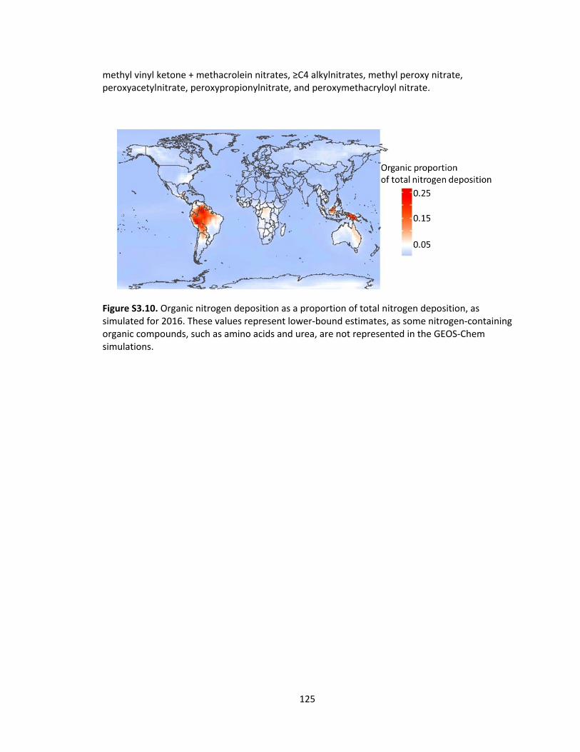
125

methyl vinyl ketone + methacrolein nitrates, ≥C4 alkylnitrates, methyl peroxy nitrate, peroxyacetylnitrate, peroxypropionylnitrate, and peroxymethacryloyl nitrate.

Figure S3.10. Organic nitrogen deposition as a proportion of total nitrogen deposition, as simulated for 2016. These values represent lower-bound estimates, as some nitrogen-containing organic compounds, such as amino acids and urea, are not represented in the GEOS-Chem simulations.

126

Appendix 3 Chapter 4 Supplemental Material

Figure S4.1. Relationship between proportion of N retained and mean annual temperature for watershed with positive net nitrogen retention value. This figure is a subset of figure 3, here detailing only watersheds with proportions of N retained greater than 0.

127

Figure S4.2. (a) Relationship between mean annual temperature and proportional N retention by permafrost coverage. Watersheds with greater permafrost coverage (continuous/discontinuous) generally retained less nitrogen. Further, temperature explained less of the variability in retention for these watersheds. (b) Map of N export measurement sites, color coded with positive versus negative retention values. Watersheds with negative retention values tended to be further north and have greater permafrost coverage.

Table S4.1. Dataset for analyzing nitrogen retention is attached as “Table S4.1.csv”. Metadata and references are below.

Table S4.1 metadata.

128

Variable name Description Units (for numerical variables)

Site Site name, as indicated in the primary literature

Location General location of site

Basin_type Categorical indicator (boreal, tundra, or glacial)

Latitude Latitude at site of nitrogen export measurement for each watershed

decimal degrees

Longitude Longitude at site of nitrogen export measurement for each watershed

decimal degrees

Period Temporal period over which quantitative variables are measured and averaged on an annual basis

Years (c.e.)

Mean_annual_temperature_C Mean annual surface air temperature in watershed. From Matsuura and Willmott (2015a)

Degrees celcius

N_retention Absolute area-normalized annual watershed nitrogen retention calculated as: (N_deposition) - (N_export)

kgN km-2 yr-1

N_export Annual area-normalized export of total nitrogen from watershed, measured at stream outlet

kgN km-2 yr-1

N_deposition Annual area-normalized atmospheric deposition of inorganic nitrogen in watershed. From Ackerman et al. 2018

kgN km-2 yr-1

Runoff_mm Annual watershed runoff mm2

Watershed_area_km2 Area of watershed km2

Permafrost_presence Binary indicator of presence/absence of permafrost within watershed. From Brown et al. (2002)

Permafrost_extent Categorical indicator of permafrost extent within watershed. From Brown et al. (2002)

Topsoil_organic_carbon_percent_weight

Organic carbon content for top 30 cm of soil (from Wieder et al. 2014)

% weight

Reference Original source for nitrogen export data and watershed description. Full citation available in Supplemental Information file.

Table S4.1 references:

Clair, T. A., Pollock, T. L., & Ehrman, J. M. (1994). Exports of carbon and nitrogen from river basins in Canada's Atlantic Provinces. Global Biogeochemical Cycles, 8(4), 441-450.

Clair, T. A., Dennis, I. F., & Bélanger, S. (2013). Riverine nitrogen and carbon exports from the Canadian landmass to estuaries. Biogeochemistry, 115(1-3), 195-211.

129

De March, L. (1975). Nutrient budgets for a high arctic lake (Char Lake, NWT) With 3 figures and 3 tables in the text. Internationale Vereinigung für theoretische und angewandte Limnologie: Verhandlungen, 19(1), 496-503.

Dittmar, T., & Kattner, G. (2003). The biogeochemistry of the river and shelf ecosystem of the Arctic Ocean: a review. Marine chemistry, 83(3-4), 103-120.

Fölster, J. (2000). The near-stream zone is a source of nitrogen in a Swedish forested catchment. Journal of environmental quality, 29(3), 883-893.

Hodson, A. J., Mumford, P. N., Kohler, J., & Wynn, P. M. (2005). The High Arctic glacial ecosystem: new insights from nutrient budgets. Biogeochemistry, 72(2), 233-256.

Kaste, Ø., & Skjelkvåle, B. L. (2002). Nitrogen dynamics in runoff from two small heathland catchments representing opposite extremes with respect to climate and N deposition in Norway. Hydrology and Earth System Sciences Discussions, 6(3), 351-362.

Kortelainen, P., Saukkonen, S., & Mattsson, T. (1997). Leaching of nitrogen from forested catchments in Finland. Global Biogeochemical Cycles, 11(4), 627-638.

Lafrenière, Melissa J., Nicole L. Louiseize, and Scott F. Lamoureux. "Active layer slope disturbances affect seasonality and composition of dissolved nitrogen export from High Arctic headwater catchments." Arctic Science 3.2 (2017): 429-450.

Lepistö, A., Andersson, L., Arheimer, B., & Sundblad, K. (1995). Influence of catchment characteristics, forestry activities and deposition on nitrogen export from small forested catchments. Water, Air, and Soil Pollution, 84(1-2), 81-102.

Likens, G. E., Bormann, F. H., Pierce, R. S., Eaton, J. S., & Johnson, N. M. (1977). The Northern Hardwood Ecosystem at Hubbard Brook in Relation to Other Forested Ecosystems in the World. In Biogeochemistry of a Forested Ecosystem (pp. 103-112). Springer, New York, NY.

Lundin, L., (1994). Impacts of forest drainage on flow regime. Technical Report. Uppsala. Sveriges lantbruksuniversitet. Studia forestalia Suecica ; 192.

MacLean, R., Oswood, M. W., Irons, J. G., & McDowell, W. H. (1999). The effect of permafrost on stream biogeochemistry: a case study of two streams in the Alaskan (USA) taiga. Biogeochemistry, 47(3), 239-267.

Mattsson, T., Finér, L., Kortelainen, P., & Sallantaus, T. (2003). Brook water quality and background leaching from unmanaged forested catchments in Finland. Water, Air, and Soil Pollution, 147(1-4), 275-298.

Peterson, B. J., Hobbie, J. E., & Corliss, T. L. (1986). Carbon flow in a tundra stream ecosystem. Canadian Journal of Fisheries and Aquatic Sciences, 43(6), 1259-1270.

Petrone, K. C., Jones, J. B., Hinzman, L. D., & Boone, R. D. (2006). Seasonal export of carbon, nitrogen, and major solutes from Alaskan catchments with discontinuous permafrost. Journal of Geophysical Research: Biogeosciences, 111(G2).

Stottlemyer, R. (1992). Nitrogen mineralization and streamwater chemistry, Rock Creek watershed, Denali National Park, Alaska, USA. Arctic and Alpine Research, 24(4), 291-303.

USGS National Water Quality Assessment Program. <https://water.usgs.gov/nawqa/>. Accessed 1 June 2017.

130

Wadham, J. L., Hawkings, J., Telling, J., Chandler, D., Alcock, J., Lawson, E., ... & Nienow, P. (2016). Sources, cycling and export of nitrogen on the Greenland Ice Sheet. Biogeosciences Discussions.

Table S4.2. Fixed effects coefficients for model of area-normalized nitrogen export. Annual runoff and a second-order coefficient for nitrogen deposition were the only factors significantly associated with export at the alpha = 0.05 level. Site was included as a random effect.

Parameter Estimate Standard Error p-value Intercept 226.688 81.110 0.007 Mean annual temperature (°C) 2.639 2.882 0.378 N deposition (kgN km-2 yr-1) -0.474 0.240 0.072 N deposition2 0.0004 0.0002 0.036 Annual runoff (mm) 0.058 0.024 0.033 Topsoil organic carbon content (%) -0.15 1.551 0.920 Permafrost extent_Discontinuous -76.374 65.564 0.249

Table S4.3. Nitrogen retention in watersheds with net nitrogen export

Of the 98 combinations of watershed and year in our overall dataset (table S1), 28 cases showed net nitrogen export, rather than retention (i.e. annual stream export of total N exceeded atmospheric inputs to the watershed). All 28 such cases were in regions of continuous or discontinuous permafrost extent. Linear mixed effects modeling (below) revealed no significant effect of mean annual temperature or permafrost extent on area-normalized nitrogen retention in these watersheds.

Parameter Estimate Standard Error p-value Intercept -5.55 5.37 0.32 Mean annual temperature (°C) -0.003 0.444 0.99 Permafrost extent_Discontinuous 2.57 4.47 0.56

Table S4.4. Representative rate measurements of nitrogen processes on an annual, per-area basis. Units for all three processes (N fixation, denitrification, and N deposition) have been converted to kgN km-2 yr-1. Value ranges represent spatial variation of the measured rate within the described location.

Process Rate Location Reference N fixation 25-30 Canadian high arctic tundra Chapin et al. 1991

80 - 131 Alaskan low arctic tundra Shaver et al. 2014 25-350 Swedish boreal forest DeLuca et al. 2008 110 Frost-heave circles in Northern

Sweden Sorensen et al. 2018

131

25 Heath vegetation Northern Sweden

Sorensen et al. 2018

88 Moss bed in Northern Sweden Sorensen et al. 2018 20-200 Tundra-wide biome estimate Stewart et al. 2014 7 - 380 Alaskan high arctic tundra Gersper et al. 1980,

Robinson & Wookey 1997 136 - 349

Northern Finland sub-arctic tundra Robinson & Wookey 1997

Denitrification 2.4 - 3.4 Alaskan high arctic Barsdate and Alexander 1975, Gersper et al. 1980

100-200 Alaskan low arctic (potential rates, unlikely to occur under field conditions)

Shaver et al. 2014

N deposition 14 - 64 Alaskan low arctic tundra Shaver et al. 2014 200 Icelandic post-glacial lavafield Jónsdóttir et al. 1995 4 - 35 Alaskan alpine tundra Vet et al. 2014 26-37 Swedish subarctic alpine tundra Bergstrom et al. 2013 40 - 110 Swedish boreal forest DeLuca et al. 2008

Table S4.4 references

Barsdate, R. J., & Alexander, V. (1975). The Nitrogen Balance of Arctic Tundra: Pathways, Rates, and Environmental Implications 1. Journal of Environmental Quality, 4(1), 111-117.

Bergström, A. K., Faithfull, C., Karlsson, D., & Karlsson, J. (2013). Nitrogen deposition and warming–effects on phytoplankton nutrient limitation in subarctic lakes. Global Change Biology, 19(8), 2557-2568.

Chapin, David M., L. C. Bliss, and L. J. Bledsoe. "Environmental regulation of nitrogen fixation in a high arctic lowland ecosystem." Canadian Journal of Botany 69.12 (1991): 2744-2755.

DeLuca, T. H., Zackrisson, O., Gundale, M. J., & Nilsson, M. C. (2008). Ecosystem feedbacks and nitrogen fixation in boreal forests. Science, 320(5880), 1181-1181.

Gersper, P. L., Alexander, V., Barkley, S. A., Barsdate, R. J., & Flint, P. S. (1980). The soils and their nutrients. An Arctic Ecosystem: The Coastal Tundra at Barrow, Alaska, 12.

Jónsdóttir, I. S., Callaghan, T. V., & Lee, J. A. (1995). Fate of added nitrogen in a moss-sedge Arctic community and effects of increased nitrogen deposition. Science of the Total Environment, 160, 677-685.

Robinson, C. H., & Wookey, P. A. (1997). Microbial ecology, decomposition and nutrient cycling. Ecology of Arctic Environments, ed. S. J. Woodin and Mick Marquiss, 41-68.

Shaver, G. R., Laundre, J. A., Bret-Harte, M. S., Chapin, F. S., Mercado-Dıaz, J. A., Giblin, A. E., ... & Gould, W. A. (2014). Terrestrial ecosystems at toolik Lake, Alaska. Alaska’s changing Arctic: Ecological consequences for tundra, streams, and lakes, ed. JE Hobbie, and GW Kling, 90-142.

132

Stewart, K. J., Grogan, P., Coxson, D. S., & Siciliano, S. D. (2014). Topography as a key factor driving atmospheric nitrogen exchanges in arctic terrestrial ecosystems. Soil Biology and Biochemistry, 70, 96-112.

Sorensen, P. L., Jonasson, S., & Michelsen, A. (2006). Nitrogen fixation, denitrification, and ecosystem nitrogen pools in relation to vegetation development in the subarctic. Arctic, Antarctic, and Alpine Research, 38(2), 263-272.

Vet, R., Artz, R. S., Carou, S., Shaw, M., Ro, C. U., Aas, W., ... & Hou, A. (2014). A global assessment of precipitation chemistry and deposition of sulfur, nitrogen, sea salt, base cations, organic acids, acidity and pH, and phosphorus. Atmospheric Environment, 93, 3-100.