Antennas and Propagation

updated: 09/29/2014

Wireless Communication Systems

Multiplexer Modulator Converter Electromagnetic Energy

Converter De modulator

De multiplexer Electromagnetic

Energy

Our focus

Antenna Characteristics

o Radiation patterns o Radiated power o Half-power beam width of the

antenna o Antenna position, shape, and length o Antenna gain with respect to an ideal

case

Remember: Antenna Properties

o  An antenna is an electrical conductor (transducer) or system of conductors n  They carry time-varying

currents and, consequently, accelerating electrons

n  à A Transmission Antenna radiates electromagnetic energy into space

n  à A Reception Antenna collects electromagnetic energy from space

radiating electromagnetic energy into space

collecting electromagnetic energy from space

Remember: Waves and Propagation - Demo

http://phet.colorado.edu/simulations/sims.php?sim=Radio_Waves_and_Electromagnetic_Fields

radiating electromagnetic energy into space

collecting electromagnetic energy from space

Anntena carry time-varying currents

Remember: Antenna Properties Reciprocal Devices

o  Most antennas are reciprocal devices, n  That is they are exhibiting the same radiation pattern

for transmission as for reception o  When operating in the receiving mode, the antenna

captures the incident wave n  Only that component of the wave whose electric field

matches the antenna polarization state is detected o  In two-way communication, the same antenna can be

used for transmission and reception n  Antenna characteristics are the same for transmitting

or receiving electromagnetic energy o  The antenna can receive on one frequency and

transmit on another

Polarization

http://www.cabrillo.edu/~jmccullough/Applets/optics.html

Start With Basics: o  We know:

n  Q (static charges) à E field– capacitor example[1] n  I (moving charges) à H field– compass example[2] n  Thus, in the presence of time-varying current à we

will obtain interdependent EM fields o  A time-varying current (I) along a wire

generates rings of Electromagnetic field (B) around the wire

o  Similarly the current passing through a coil generates Electromagnetic field in the Z axis

[2] http://micro.magnet.fsu.edu/electromag/java/compass/index.html

[1] http://micro.magnet.fsu.edu/electromag/electricity/capacitance.html

Simple Experiments

Faraday’s Law: Electromotive force (voltage) induced by time-varying magnetic flux:

An induced magnetic field

Faraday confirmed that a moving magnetic field is necessary in order for electromagnetic induction to occur

Galvanometer needle moves

Electromagnetic field (B)

1

2

3

Maxwell Equations o  Gauss’s Law o  Faraday’s Law o  Gauss’s Law for Magnetism o  Ampere’s Law

Relationships between charges, current, electrostatic, electromagnetic, electromotive force!

Maxwell’s Equations – Free Space Set

o We assume there are no charges in free space and thus, = 0 Time-varying E and

H cannot exist independently!

If dE/dt non-zeroà dD/dt is non-zero

àCurl of H is non-zero à D is non-zero

(Amp. Law)

If H is a function of time à E must exist!

(Faraday’s Law)

Interrelating magnetic and electric fields!

Our Focus: Far-Field Approximation

1. In close proximity to a radiating source, the wave is spherical in shape, but at a far distance, it becomes approximately a plane wave as seen by a receiving antenna. 2. The far-field approximation simplifies the math. 3. The distance beyond which the far-field approximation is valid is called the far-field range (will be defined later).

Very similar to throwing a stone in water!

dfar_field=(2*l2)/λ

far-field range

What is the power radiated? A far field approximation

o  Assuming the alternating current travels in Z directionà radiated power must be in Z

o  Antenna patterns are represented in a spherical coordinate system

o  Thus, variables R, θ, φ à n  range, n  zenith angle (elevation), n  azimuth angle

http://www.flashandmath.com/mathlets/multicalc/coords/shilmay23fin.html

Hertzian Dipole Antenna o  Using Ampere’s Law

o  But how is the current I(r) distributed on the antenna?

o  One way to approximate this rather difficult problem is to use thin-wire dipole antenna approximation n  Dipole because we have two poles (wires) n  a<<L

o  We only consider the case when L is very very short (Hertzian Dipole) n  Infinitesimally short n  Uniform current distribution

http://whites.sdsmt.edu/classes/ee382/notes/382Lecture32.pdf

Hertzian Dipole (Differential Antenna) Radiation Properties

o Very thin, short (l<λ/50) linear conductor

o Observation point is somewhere in the space

http://www.amanogawa.com/archive/Antenna1/Antenna1-2.html

Hertzian Dipole (Differential Antenna) Radiation Properties

Note that:

K=wave number

ω = 2π f ;k =ω / c = 2π f / c = 2π / λ;l << λ / 50;R ≈ R' = Γ;

ε  is the free space permittivity (about 1) µ  is magnetic Permeability η is the intrinsic impedance in Ohm

η0 = µ0 /ε0 =120π;

Hertzian Dipole (Differential Antenna) Radiation Properties

In this case: 1/Rà radiation field components 1/R^2àinduction field components 1/R^3àelecrostatic field components Far-field à only radiation field! à Only Eθ and Hφ will be significant!

A/m

V/m

R= Range θ=Zenith (elevation) – side view φ=Azimuth – top view

Hertzian Dipole (Differential Antenna) Radiation Properties

A/m

V/m

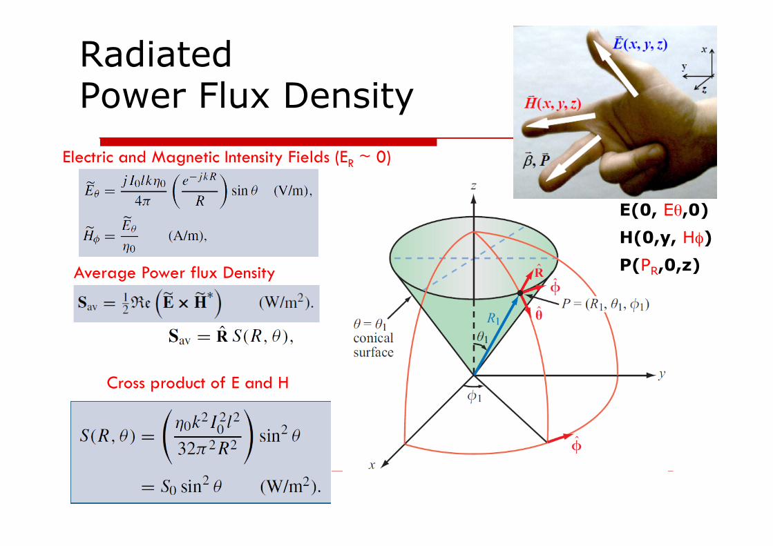
Radiated Power Flux Density

Electric and Magnetic Intensity Fields (ER ~ 0)

Average Power flux Density

Cross product of E and H

E(0, Eθ,0)

H(0,y, Hφ)

P(PR,0,z)

Normalized Radiation Intensity(F) Normalized Radiation Intensity àHow much radiation in each direction?

So=Smax= Max. Power Density

R= Range θ=Zenith (elevation) – side view φ=Azimuth – top view

Elevation Pattern (side view)

Azimuth Pattern (top view)

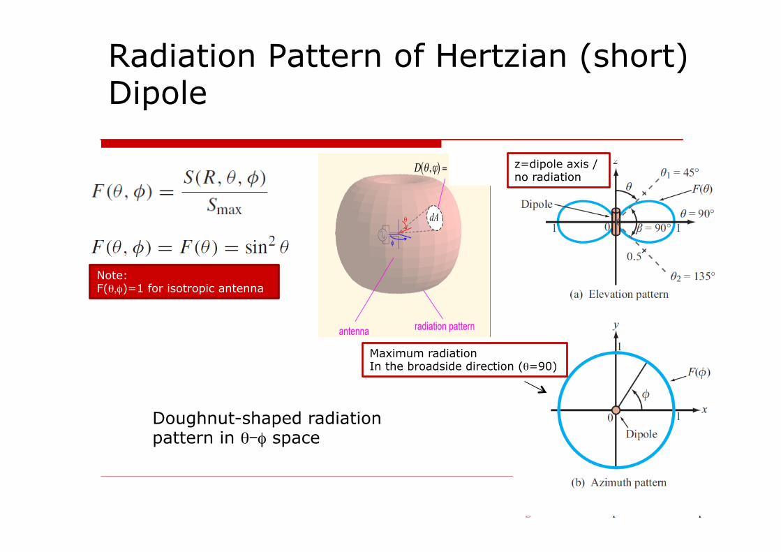
Radiation Pattern of Hertzian (short) Dipole

Doughnut-shaped radiation pattern in θ-φ space

z=dipole axis / no radiation

Maximum radiation In the broadside direction (θ=90)

Note: F(θ,φ)=1 for isotropic antenna

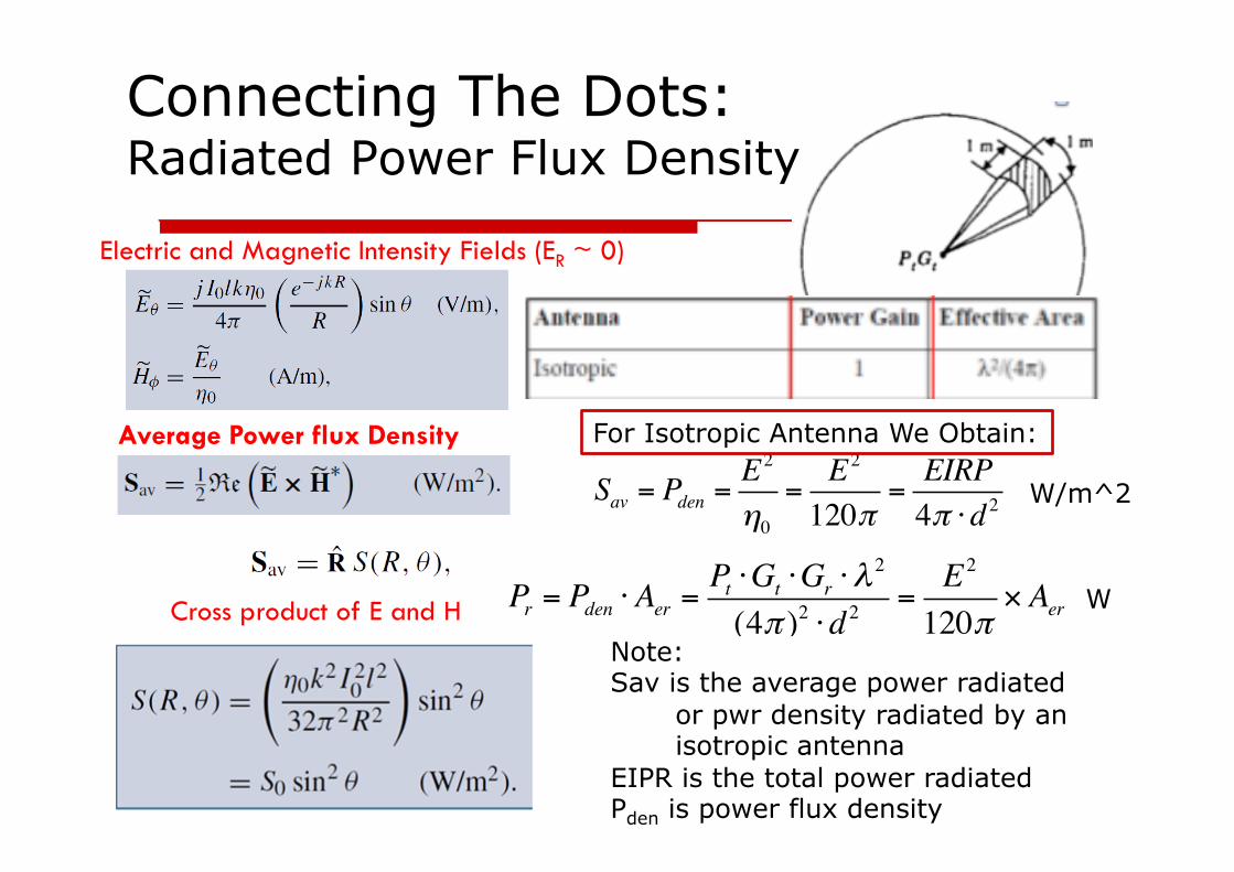
Electric and Magnetic Intensity Fields (ER ~ 0)

Average Power flux Density

Cross product of E and H

Sav = Pden =E 2

η0=

E 2

120π=EIRP4π ⋅d 2

W/m^2

Pr = Pden ⋅Aer =Pt ⋅Gt ⋅Gr ⋅λ

2

(4π )2 ⋅d 2=

E 2

120π× Aer W

For Isotropic Antenna We Obtain:

Connecting The Dots: Radiated Power Flux Density

Note: Sav is the average power radiated or pwr density radiated by an isotropic antenna EIPR is the total power radiated Pden is power flux density

Example o  Example A (Hertzian Dipole) o  Example B (Isotropic Antenna)

Antenna Directionality o  Set the wavelength to 1 o  Set Current to 1 A o  Plot Power o  Change the length o  Q1: What happens to the

directivity when l changes? o  Q2: What happens to the

power when L changes?

http://www.amanogawa.com/archive/DipoleAnt/DipoleAnt-2.html

The magic is all here:

Other Antenna Properties o We already looked at the radiation

intensity and radiation pattern o Other properties

n  Radiation Pattern Characteristics n  Radiation Resistance

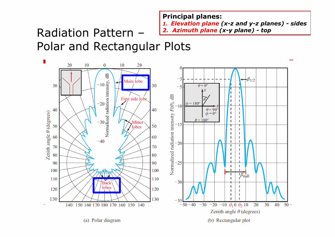
Radiation Pattern – Polar and Rectangular Plots

Principal planes: 1. Elevation plane (x-z and y-z planes) - sides 2. Azimuth plane (x-y plane) - top

Radiation Pattern Beamwidth Dimensions

Null Bandwidth & Half-power beamwidth

Since 0.5 corresponds to ‒3 dB, the half power beamwidth is also called the 3-dB beamwidth.

Half-power angles: theta1 and theta2

Half-power beamwidth

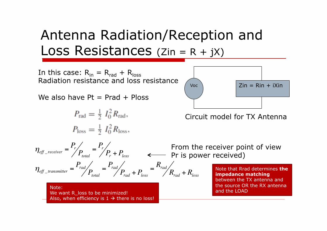
Antenna Radiation/Reception and Loss Resistances (Zin = R + jX)

Note: We want R_loss to be minimized! Also, when efficiency is 1 à there is no loss!

ηeff _ receiver =PrPtotal

= Pr Pr +Ploss

ηeff _ transmitter =Prad

Ptotal= Prad Prad +Ploss

= Rrad Rrad + Rloss

In this case: Rin = Rrad + Rloss Radiation resistance and loss resistance We also have Pt = Prad + Ploss

Voc

Circuit model for TX Antenna

From the receiver point of view Pr is power received)

Note that Rrad determines the impedance matching between the TX antenna and the source OR the RX antenna and the LOAD

Zin = Rin + iXin

Gain, Directivity, Power Radiated & Rrad

For any antenna:

For the Hertzian dipole:

D =4πR2SmaxP rad

=SmaxSav

G =ηeff .D

Directionality & Gain

Prad =4πR2Smax

DAssuming there is no ohmic loss (lossless antenna)

Power Gain = 1.5

Smax

Smax is the average power radiated or pwr density radiated by an antenna

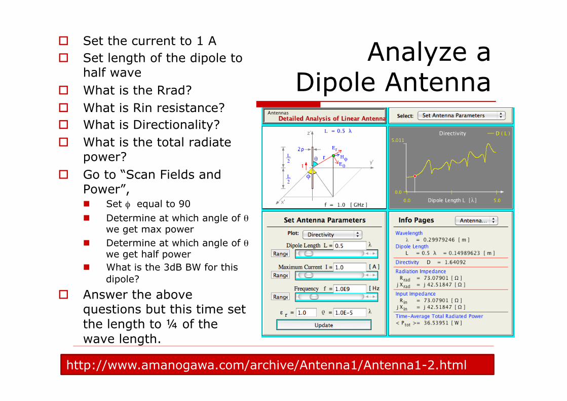
Analyze a Dipole Antenna

o  Set the current to 1 A o  Set length of the dipole to

half wave o  What is the Rrad? o  What is Rin resistance? o  What is Directionality? o  What is the total radiate

power? o  Go to “Scan Fields and

Power”, n  Set φ equal to 90 n  Determine at which angle of θ

we get max power n  Determine at which angle of θ

we get half power n  What is the 3dB BW for this

dipole?

o  Answer the above questions but this time set the length to ¼ of the wave length.

http://www.amanogawa.com/archive/Antenna1/Antenna1-2.html

Example o  Example C (Measuring the received power) o  Example D (Resistance loss in a short dipole) o  Example E (rewrite the average power density in terms

of current, distance between the two antennas, length of the antenna, and frequency of operation for a short dipole (loop)

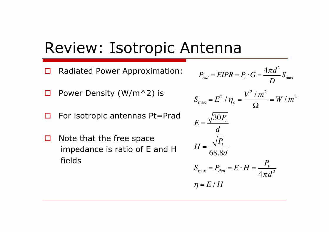
Review: Isotropic Antenna o  Radiated Power Approximation:

o  Power Density (W/m^2) is

o  For isotropic antennas Pt=Prad

o  Note that the free space impedance is ratio of E and H fields

Prad = EIPR = Pt ⋅G =4πd 2

DSmax

Smax = E2 /ηo =

V 2 /m2

Ω=W /m2

E =30Ptd

H =Pt

68.8d

Smax = Pden = E ⋅H =Pt4πd 2

η = E /H

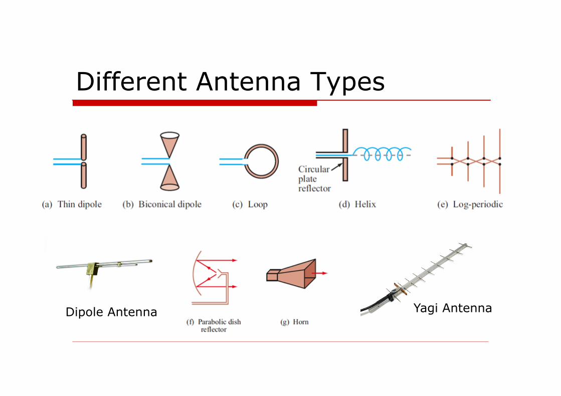
Different Antenna Types

Yagi Antenna Dipole Antenna

Fields in Half-Wave Dipole Homework Assignment

•  Example F: Find the following: •  Find the expression for average power

density •  Power Density (Smax) •  Normalized radiation intensity, F •  Directionality, D (from the table) •  P_radiated •  R_radiated •  Prove that 3dB BW is in fact 78 degrees

(you can use substitution to prove! •  HINT: Use the applet to check your

answers All works must be shown!

Example: Complete the Table Below Antenna Gt=D Rrad Prad 3dB BW Eff. Area

Isotropic ---------- ---------- --------- ---------- ----------

Short Dipole ½ Wave

¼ Wave Later Later Later Later Later

Example G

Why dBi = dBd + 2.15dB? Explain!

References o  Ulaby, Fawwaz Tayssir, Eric Michielssen, and Umberto

Ravaioli. Fundamentals of Applied Electromagnetics: XE-AU.... Prentice Hall, 2001, Chapter 9

o  Black, Bruce A., et al. Introduction to wireless systems. Prentice Hall PTR, 2008, Chapter 2

o  Rappaport, Theodore S. Wireless communications: principles and practice. Vol. 2. New Jersey: Prentice Hall PTR, 1996, Chapter 3

o  Wheeler, Tom. Electronic communications for technicians. Prentice Hall, 2001. Section 12-1 & 12-2