Answers to Selected Problems

Chapter 2

1. (a) Physical; (b) – (d) physical plus environmentally assisted.2. Anodic: Zn (s)→ Zn2+ (aq) + 2e−

Cathodic: 2H+ (aq) + 2e− → H2 (g)and: O2 (g) + 2H2O (l) + 4e− → 4OH−

3. Anodic: Fe (s)→ Fe2+ (aq) + 2e−and: Cr(s)→ Cr3+ (aq) + 3e−Cathodic: O2 (g) + 2H2O (l) + 4e− → 4OH−

4. (a) Anodic: Cu (s)→ Cu2+ (aq) + 2e−Cathodic: O2 (g) + 2H2O (l) + 4e− → 4OH−

(b) Precipitation occurs.(c) Decreasing the pH increases the concentration of H+ ions and decreases the concentration

of OH− ions so that the equilibrium is shifted to the left.6. 93.1 mA/cm2.7. (a) 3.97 × 10−4 g/(cm2 h); (b) 0.363 mA/cm2.8. (a) 7.40 × 10−3 A/m2; (b) 8.23 × 10−3 mm/year; (c) 61 years.9. 5.9 mils thickness required.

10. 0.664 mA/cm2.11. Hf has the larger atomic weight and thus the larger weight loss.12. The final pH is 14.4. Figure 2.11 shows that this will cause an increase in the corrosion rate of

Al.13. (a) Anodic areas usually appear near the point of the nail. (b) The bent part of the nail is an

anodic area because straining the metal perturbs metal atoms from their equilibrium latticepositions.

Chapter 3

1. The number of water molecules involved in primary hydration is 0.86% of the total watermolecules.

2. 2.5 × 107 V/cm.3. (a) 75 μF/cm2; (b) 56 μF/cm2; (c) 30 μF/cm2.4. V = PD M1/S − PD ref/S.6. (a) E = −0.380 V vs. SCE; E = −0.360 V vs. Ag/AgCl; (c) E = −0.454 V vs. Cu/CuSO4.

521E. McCafferty, Introduction to Corrosion Science, DOI 10.1007/978-1-4419-0455-3,C© Springer Science+Business Media, LLC 2010

522 Answers to Selected Problems

8. (a) False; (b) True; (c) True.9. (a) False; (b) True; (c) False.

10. The double-layer capacitance Cdl decreases as the corrosion rate decreases, and thus can be usedto monitor the corrosion rate.

11. The double-layer capacitance per unit area Cdl is given by Cdl = ε/d. As an organic moleculeadsorbs, ε decreases and the thickness d of the edl increases, so that Cdl decreases.

Chapter 4

2. (a) 1364 cal/mol; 5708 J/mol.3. (a) E = +0.235 V vs. SHE. (b) The electrode potential for the SCE electrode is + 0.242 V vs.

SHE, so there is only 7 mV difference between the two.4. E = −0.337 V vs. SHE.5. E = +0.209 V vs. SHE.6. The reaction is spontaneous.7. (a) The overall reaction is spontaneous in the standard state; (b) E0 = +0.656 V vs. SHE; (c)

E = 0.656 + 0.0295 log [MoO42−] − 0.0.0591 pH; (d) the overall reaction to form MoO2 is

spontaneous, under the given conditions; and (e) Spontaneity of forming MoO2 depends on theexperimental conditions, i.e., pH and MoO4

2− concentration.8. μ0 (Sn2+ (aq)) = − 26,634 J/mol = −6365 cal/mol.9. E = −2.394 V vs. SHE.

10. [Pb+2] = 0.036 M.11. We cannot add the two given values of E0. We must write �G0 =−nFE0 =�(νiμi

0 (products))− �(νiμi

0 (reactants)) for each of the two given half-cell reactions to calculate μ0(Fe2+) andμ0(Fe3+) for use in calculating E0 (Fe3+/Fe). The result is E0 (Fe+3/Fe) = −0.041 V vs. SHE.

12. In the solid metal, a metal atom is confined to a certain lattice position. In the aqueous solution,the metal cation can move through the solution, so the disorder increases. Thus, the entropyincreases.

Chapter 5

1. (a) The nickel electrode is the anode and will corrode; (b) cell emf is +0.570 V; (c) Ni (s) + Cu2+

(aq)→ Cu (s) + Ni2+ (aq).2. (a) The aluminum electrode is the anode and will corrode; (b) cell emf is +1.391 V; (c) 2Al (s)

+ 3Ni2+ (aq)→ 2Al3+ (aq) + 3Ni (s).3. [Cd2+]/[Fe2+] = 0.032.4. (a) Pb in contact with 0.01 M Pb2+ is the anode. (b) Cell emf is +0.05 V.5. (a) Zn is more negative in the emf series and in the galvanic series for seawater. (b) Sn is more

negative than Cu in the emf series, but both have approximately the same potential in seawater.(c) Ni is more negative than Ag in the emf series, but both have approximately the same potentialin seawater. (d) Ti is more negative than Fe in the emf series, but is more positive in the galvanicseries for seawater.

6. (a) Mg can be used to cathodically protect steel in seawater. (b) Al can be used to cathodicallyprotect steel in seawater. (c) Either Be or Cd can be used to cathodically protect steel in seawater.

7. Tin will be the anode and will corrode to protect the underlying steel substrate.

Answers to Selected Problems 523

8. (a) Aluminum will be the anode. (b) No galvanic effect. (c) Potentials are near each other sothat a galvanic effect is not likely. (d) Aluminum will be the anode.

9. The electrode potential of the second-phase particle Al2CuMg is more negative than thealuminum matrix, so the second-phase particle will preferentially corrode. However, thealuminum matrix has an electrode potential more negative than the second-phase particleAl3Fe, so that the aluminum matrix will corrode in a galvanic couple between Al andAl3Fe.

10. Cadmium is a sacrificial coating, and Cd will corrode if a break develops in the coating down tothe steel substrate.

11. If a break develops in the stainless steel coating and extends down to the plain steel substrate,the steel substrate will galvanically corrode.

12. (a) If a break develops down to the Cr layer, Cr will corrode. (b) If the break continues down tothe steel substrate, the steel substrate will corrode.

13. Case B is worse. This situation involves a large area cathode connected to a smaller areaanode, so that the anodic current density will be increased at the surface of the steel nut andbolt. Case B is the less troublesome situation of a small cathode connected to a larger areaanode.

14. Waterline corrosion below the surface is possible due to the operation of an differential oxygencell.

Chapter 6

1. (a) Mild steel lies just within a region of corrosion; zinc lies in a region of corrosion.(b) Coupled mild steel lies in a region of immunity; coupled zinc lies in a region of cor-rosion. (c) These results are consistent with predictions based on the galvanic series forseawater.

2. Corrosion of silver at pH 5 occurs between approximately 0.45 and 1.1 V vs. SHE.3. The region of corrosion as Pd2+ ions lies above the “a” line for H2 evolution. Thus, H2 is not

stable in this region of Pd corrosion, so the reaction of Pd with H+ ions to form H2 is notthermodynamically favored.

4. (b) Three methods of protection are (i) increase the electrode potential into a region of pas-sivity (anodic protection), (ii) make the electrode potential more negative to move into aregion of immunity (cathodic protection), (iii) increase the pH to move into a region ofpassivity.

5. 96.5 min.6. E0 = −1.550 V vs. SHE.

10. E = 1.311 + 0.0197 log [CrO42−] − 0.0985 pH

11. (a) Ti (s) + H2O (l)→ TiO (s) + 2H+ (aq) + 2e−; 2TiO (s) + H2O (l)→ Ti2O3 + 2H+ (aq) +2e−; Ti2O3+ H2O (l)→ 2TiO2 (s) + 2H+ (aq) + 2e− (b) dE/dpH = −0.0591 for each of thethree reactions.

12. The Pourbaix diagram for Mg is similar in general shape to that for Al or Zn (Figs. 6.1 and 6.7).14. The electrode potential must be more positive than −0.177 V vs. SHE.15. The data point lies below the “a” line for H2, so that H2 gas is stable under the experimental

conditions and is likely the gas which was observed.16 Nb and Ta have similar Pourbaix diagrams. Nb and Ta appear in the same column in the Periodic

Table and are expected to have similar chemical behavior. (See Fig. 9.24.)

524 Answers to Selected Problems

Chapter 7

1. (a) 0.411 g/cm2 h; (b) 123 mA/cm2.2. (a) 71.3 mg/cm2 year. (b) The corrosion rate decreases with time. (c) The rust layer becomes

more protective with time.3. (a) 7.5 × 10−3 M/L; (b) 0.10 g/cm2; (c) 41.9 mL (STP)/cm2.4. 3.6 mg/cm2 h.5. The weight fractions of metals in the alloy are Fe 0.058, Cr 0.162, Mo 0.153, Ni 0.546. Their

cation fractions in solution are Fe 0.057, Cr 0.100, Mo 0.130, Ni 0.712. Thus, Ni is preferentiallycorroded, while the others are not.

6. ba = 0.0591 V.8. (a) Ecorr = −0.459 V vs. SCE. (b) icorr = 24 μA/cm2.9. (a) The overvoltage is given by η = 0.0591/n (in V), where n is the number of electrons trans-

ferred. If n = 1, η = 0.0591 V. If n = 2, η = 0.0296 V. (b) η = 0.118/n (in V), where n is thenumber of electrons transferred. If n = 1, η = 0.118 V. If n = 2, η = 0.0591 V.

10. log icorr = (1/2) log (Ac/Aa) + constant.11. (a) icorr = 1.2 × 10−5 A/cm2 (b) Ecorr = −0.03 V12. 1.6 μA/cm2.13. ba = 0.073 V.

Chapter 8

1. (a) 0.0173 cm; (b) 2005 jumps/s.2. 3.7 h.3. 5.6 h.4. 35 s (using 0.065 cm as the thickness δ of the diffusion layer from Example 8.2).5. For δ = 0.05 cm, iL = 3.9 × 10−5 A/cm2. For δ =0.1 cm, iL = 1.9 × 10−5 A/cm2. (Using D =

2.0 × 10−6 cm2/s and the concentration of dissolved O2 = 8.0 mg/L from Fig. 8.5.)6. (b) Increasing the flow velocity increases the limiting cathodic current density iL for the reduc-

tion of oxygen and hence increases the corrosion rate. (c) The concentration of dissolved O2decreases, so iL decreases and so does the corrosion rate.

7. The following assumptions must hold: (i) the only cathodic reaction is the reduction of O2,(ii) the O2 reduction reaction is under diffusion control, and (iii) the anodic and cathodicpolarization curves intersect in the region of the limiting cathodic current density.

8. (b) Ecorr = −0.070 V vs. SHE = −0.31 V vs. SCE. (c) From the galvanic series for seawater,Ecorr = −0.1 to −0.2 V vs. SCE.

9. (a) 11 μA/cm2; (b) 3.1 g/m2 day.10. The electrolyte in contact with the hotter end of the metal will contain less dissolved O2

(Fig. 8.4). Thus, an oxygen concentration cell will be set up, with the hotter end of the metalbecoming the anode.

11. 238 μA/cm2.

Chapter 9

1. 0.94−1.91 monolayers of O−2.2. The calculated potential for the reduction of γ-Fe2O3 to Fe2+ is −0.214 V vs. SHE., in good

agreement with the experimental value for the first plateau. The calculated potential for the

Answers to Selected Problems 525

reduction of Fe3O4 to Fe is −0.534 V vs. SHE., in good agreement with the experimental valuefor the second plateau.

3. Tantalum. Based on the Pourbaix diagrams in Fig. 9.24, tantalum is either passive or immuneover a large range of pH and electrode potential.

4. E = −0.672 V vs. SHE; not in agreement with the experimentally observed Flade potential.6. 15.9 at.% Ni. The electron configuration theory is based on the concept of an adsorbed film and

does not take into account the properties of the oxide film.7. The effective molecular weight of the oxide is 136.17 g/mol. The effective atomic weight

of the metal is 55.27 g/mol. The effective value of n = 1.74. The density of the oxide is6.67 g/cm3. The density of the metal is 7.0 g/cm3 (given). R = 1.49, so that the oxide film isprotective.

8. The addition of Mo to Fe–Ni alloys is predicted to be detrimental. This trend is in agreementwith the text, which states that Mo is beneficial only when Cr is present.

9. (a) icorr ≈ 400 μA/cm2; (b) 0 to +0.3 V vs. SCE; (c) 30 μA/cm2; (d) 9.5× 10−4 cm penetration;(e) at −0.7 V vs. SCE, ianodic ≈ 30 μA/cm2.

10. (a) The anodic and cathodic polarization curves intersect in a region of active corrosion. (b) Theanodic and cathodic curves intersect in a region of passivity. (c) The situation is unstable andthe system oscillates between a state of active corrosion and one of passivity.

Chapter 10

1. Pitting and crevice corrosion are similar in their propagation stages. Each of these two formsof localized corrosion results in the formation of an internal solution of low pH and concen-trated in Cl− ions and in metal cations. Pitting and crevice corrosion differ in their initiationstages. Crevice corrosion initiates by means of a differential O2 cell, whereas pitting involvesthe localized breakdown of an oxide film (by one of several different mechanisms).

3. (c) Both the 1.0 cm2 crevice and the 2.0 cm2 crevice have the same weight loss, but the smallersample has the greater weight loss per unit area.

6. The pitting potential is Epit = −0.70 V vs. S.C.E.7. The current density within the pit is approximately 1,900 A/cm2.8. (a) The pitting potential for pure Al in 0.6 M Cl− is−0.74 V vs. S.C.E.=−0.72 V vs. Ag/AgCl.

(b) The pitting potential of Al alloys in seawater from Table 10.5 is −0.88 V vs. Ag/AgCl.(c) Agreement is fair. Differences may be caused by the following reasons: (i) Use of 0.6 M Cl−does not satisfactorily simulate seawater, which contains other ions as well as organic matter.(ii) Short-term laboratory tests do not represent data obtained over a much longer period ofimmersion. (iii) We have considered laboratory data for pure Al rather than for the Al alloy ofinterest.

9. (b) Safe ranges are more negative than −0.7 V vs. SCE (immunity) or between −0.35 V and−0.58 V vs. SCE. (perfect passivity).

10. Alloy B (but not alloy A) can be used instead of 304 stainless steel. Alloy B has ahigher pitting potential in 1 M HCl than does the other two alloys and has a critical cur-rent density for passivation similar to that for 304 stainless steel and lower than that ofalloy A.

11. With increased temperature the rate increases for all individual steps which lead to pitting. Thisincludes the rate of Cl− transfer within the oxide film, the rate of oxide thinning, and the rate ofelectrochemical reactions at the metal/oxide interface. Thus, the metal can be driven to a lowerelectrode potential to cause pitting to occur.

526 Answers to Selected Problems

Chapter 11

2. KI = 38 MPa√

m.4. Crack length 2a = 0.10 in. = 2.5 mm.5. (a) KIscc = 45 ksi

√in.; (b) σ = 51 ksi; (c) KI = 19 ksi

√in. is less than KIscc so that fracture

does not occur.6. Smooth specimens do not fracture below the threshold yield stress σ th = 48 MPa. For pre-

cracked specimens, the stress is given by σ = 3.103/√

a. Pre-cracked specimens do not fracturebelow the intersection of this line and the yield stress, σY = 410 MPa. The safe-zone region liesbelow the intersection of the lines σ = 3.103/

√a and σ th = 48 MPa.

7. Making the electrode potential more negative decreases KIscc (or increases the susceptibility tostress-corrosion cracking). (If KIscc decreases, the critical flaw size also decreases for the sameapplied stress σ .) Hydrogen embrittlement is a possible mechanism of stress-corrosion crackingbecause the alloy is more susceptibile with increasing negative potentials, where more cathodiccharging with hydrogen gas can occur.

8. 1.2 A/cm2.9. The time to failure decreases for both cathodic and anodic currents. Thus, the mechanism

for stress-corrosion cracking must be a mixed-mode mechanism, involving both hydrogenembrittlement and anodic dissolution within the crack.

11. 1,563 cycles.

Chapter 12

2. For 1 M HCl, %I = 88%; for 4 M HCl, %I = 60%.3. A plot of C/θ vs. C gives a straight line of unit slope.4. Calculate θ from θ = (i0 − i)/(i0 − isat). Then, a plot of θ vs. log C gives a straight line over

a portion of the plot, indicative of a Temkin isotherm. Various tests for the Langmuir isothermfail.

6. (a) The S-containing compound is better because the S atom is a better electron donor than the Natom. (b) CH3(CH2)16COOH is better because it has the longer chain length and thus presentsa greater barrier to the aqueous solution when a close-packed monolayer is formed on the metalsurface. (c) Both compounds have similar base strengths, but the diamine (second compound)is better because it offers more attachment possibilities to the metal surface. Either of the two-NH2 groups can adsorb with the molecule in the vertical configuration or both -NH2 groupscan adsorb with the molecule being in the flat configuration. (d) The -CH3 compound (secondcompound) is better. This is because the p-CH3 group is an electron donor and provides electronsto the ring. The Hammet sigma value σ(p-CH3) = −0.17. The Cl-containing compound is anelectron acceptor and withdraws electrons from the ring. The Hammet sigma value for the Clgroup is σ(p-Cl) = +0.23. (e) The second compound is better. It contains two electron-donatinggroups, so that the electron density on the N atom is higher for the second compound.

8. (a) For the conditions given, E = +1.103 V vs. SHE for chromate reduction, and E =−0.153 V vs. SHE For tungstate reduction, (b) under the given conditions, chromate reductionis spontaneous, but tungstate reduction is not, by �G = −nFE.

9. The corrosion of metals in nearly neutral solutions differs from that in acidic solutions for tworeasons. (1) In acid solutions, the metal surface is oxide-free, but in neutral solutions, the sur-face is oxide-covered. (2) In acid solutions the main cathodic reaction is hydrogen evolution,

Answers to Selected Problems 527

but in air-saturated neutral solutions, the cathodic reaction is oxygen reduction. In each case theinhibitor must interact with the metal or oxide-covered metal surface. For acid solutions, adsorp-tion alone may be sufficient to cause inhibition. But in nearly neutral solutions, the inhibitormust be able to enhance the protective properties of the oxide film. Possibilities include (i) for-mation of surface chelates, (ii) incorporation into the film of an oxidizing inhibitor (such asCrO4

2−), which itself is reduced to Cr2O3, (iii) incorporation of the inhibitor into the oxide filmor into its pores, (iv) formation of a precipitate on the oxide film.

10. If the inhibitor does not completely cover the metal surface, there can be a difference inpotential between the covered sites and the uncovered sites. This difference can cause a gal-vanic effect, so that the uncovered sites act as local anodes, and thus localized corrosion mayoccur.

Chapter 13

1. When an anodic site is activated beneath an organic coating, the local solution becomes acidifiedand chloride ions migrate into the vicinity of the site, as in crevice corrosion. The cathodic reac-tion (O2 reduction) also occurs beneath the organic coating. This is different than the usual caseof crevice corrosion, in which the principal cathodic reaction takes place outside the crevice.The major damage to the organic coating is caused in alkaline regions (cathodic) rather than inthe acidic region (anodic). This is different than the usual case of crevice corrosion where themain corrosion damage occurs within the crevice (anodic region).

2. Filiform corrosion is different in its geometric appearance than the usual type of underfilmcorrosion, but the mechanism of detachment is similar in both cases. Cathodic regions beneaththe coating exist in each case and can give rise to cathodic delamination.

5. (a) 33,000 layers of H2O molecules, (b) 9.9% of the thickness of the organic coating containsH2O molecules.

6. (a) In 1 day the coating will transmit 1.67× 10−4 mol H2O, as compared to 7.81× 10−8 mol O2.To use up all the H2O, we would need 8.4 × 10−5 moles O2, but we have much less. Thus, O2is the limiting reactant. (b) 0.35 μA/cm2.

7. (a) The data point lies in the region of the Pourbaix diagram for aluminum where Al goes intosolution as AlO2

−. (b) Thus, the oxide film is not stable so that dissolution of the oxide isa possible mechanism of delamination. However cathodic delamination due to failure of thepolymer in the alkaline environment cannot be ruled out.

8. 92 mg/cm2 day.9. From Figs. 13.9 and 13.10, poly(vinyl acetate) is a basic polymer and poly(vinyl fluoride) is

an acidic polymer. Thus, the basic polymer, poly(vinyl acetate), would be expected to have thegreater adhesion to the acidic oxide.

10. (a) Desirable properties are that polytetrafluoroethylene (PTFE) has good corrosion resistancein most solutions and is also a hydrophobic polymer which is not wetted by aqueous solutions.In addition, PTFE has a low coefficient of friction and is a good electrical insulator. (b) Anundesirable property is that when drastically overheated, PTFE can release toxic gases. In addi-tion, perfluorooctanoic acid, which is used to make PFTE, is a carcinogen. It is also difficult toget PTFE to adhere to the metal substrate without using certain adhesion promoters. (Adhesionpromoters are often bifunctional chemical agents which act as molecular bridges between twochemically different materials. Adhesion promoters improve adhesion by chemically bondingto both types of materials simultaneously.)

528 Answers to Selected Problems

11. (a) Measuring the electrode potential of an underground coated system would be useful in find-ing holidays (breakthroughs) in the coating. (b) Similarly, measuring the polarization resistanceof specimens of the coated metal could give information on the integrity of the coating. Valuesof Rp would decrease if there is a breakthrough in the coating.

Chapter 14

7. |Z| = [R2 + 1/(ω2C2)]1/2.8. 12 μA/cm2.9. Rp = 1,910 �; Rs = 10 �, Cdl = 3.1 × 10−5 F.

10. The low-frequency value of |Z| is the parameter of interest because it contains the values of thepolarization resistance Rp and the pore resistance Rcp of the coating. |Z| → Rp + Rcp + Rs asω → 0. At low frequencies, |Z| is larger when either plasticizer is contained in the organiccoating. Benzyl alcohol is the better of the two plasticizers.

11. 4.4 × 10−7 F/cm2.

Chapter 15

1. Based on thermodynamics, there will be an increase in the stability of the oxide. When iron isalloyed with aluminum, the oxide will be a mixed oxide consisting of Fe2O3 and Al2O3, withAl2O3 being more stable than Fe2O3, per the Ellingham diagram.

2. (a) K = 1/PO2 ; (b) PO2 = 1.0 × 10−10;(c) the two results are the same.3. PO2 = 1.2 × 10−41 atm, so that oxidation is possible in air at 1,200 K.4. The observation that dust particles become enveloped within the rust layer means that the rust

layer grows both from the outside oxide surface inward and from the metal surface outward.This is similar to the Wagner mechanism of high-temperature oxidation.

6. (a) According to the Ellingham diagram, the addition of Al to Ni should result in a more stablealloy. But the oxidation rate increases with Al content, in disagreement with the Ellinghamdiagram. (b) From Table 15.5, NiO is a p-type oxide with cation vacancies. From the Haufferules in Table 15.6, a solute of higher oxidation number (Al3+) results in an increase in oxidationrate, in agreement with the Hauffe rules.

7. (a) 5.0 × 10−3 g/cm2 after 20 h; (b) 7.5 μm.8. According to Table 15.5, Al2O3 is an n-type oxide with anion vacancies. The addition of a solute

like Li+ with an oxidation number lower than that of Al3+ causes an increase in the oxidationrate, according to the Hauffe rules in Table 15.6.

9. The parabolic rate law gives the best fit.10. 37.7 mg/cm2.11. (a) Replacing U4+ with Al3+ reduces the oxidation rate. (b) Replacing U+4 with Ta+5 increases

the oxidation rate.12. krational = 6.7 × 10−9 equiv cm−1s−1.

Chapter 16

1. (a) ia/F = k3θOH−;(b) k1k2/{(k1 + k−1β) (k−2[H+])};(c) ba = 0.118 V; (d) zH+ = −1.2. 2.5 mA/cm2.

Answers to Selected Problems 529

3. 5.0 × 10−4�−1cm−1.4. Surface charges at pH 7.0 are MoO3 negative, ZrO2 negative, CdO positive.5. Surface charges at pH 11.0 are MoO3 negative, ZrO2 negative, CdO negative.6. At pH 8.0, the oxide-covered surface has a positive charge. Thus, a negatively charged corrosion

inhibitor can be adsorbed at pH 8.0.7. (a) The concentration of implanted Cr3+ ions at the surface is 33 at.%. (b) This concentration is

higher than the critical concentration of 13 at.% Cr required for passivity in Fe–Cr binary alloys.8. (a) At pH 6.0, the surface of oxide-covered copper has a positive charge. We want to implant

copper with a metal whose oxide will have a negative charge at pH 6.0 in order to replace aportion of the positively charge surface with negative charges (to minimize Cl−uptake). Thus,any oxide having an isoelectric point less than 6.0 will do. Possibilities are Ce, Ti, Ta, Si, andMo. (b) We are assuming that the implanted ion is contained in the oxide film and that theisoelectric point for an oxide film is similar to that for bulk oxides.

9. (a) In neutral solutions, the surface of oxide-covered Fe is positively charged, and surface ofoxide-covered Si is negatively charged. Thus implantation of Si into Fe will convert a portionof the positively charged surface into negative charges. The uptake of Cl− will be reduced, soprotection against pitting will be increased. (b) Fe2O3 is an n-type semiconductor with anionvacancies (Table 15.6). Insertion of Si4+ ions will decrease the concentration of anion vacancies(Table 15.6). This reduces ionic diffusion through the oxide film so that protection against pit-ting will be increased. (c) Each argument is consistent with the other, so we can conclude thatimplantation of Si into Fe provides increased resistance to pitting.

10. Ion implantation has the following limitations: (i) the depth of the modified region is shallow(hundreds to thousands of angstroms); (ii) ion implantation is a line-of-sight process so thatrecesses in the sample geometry cannot be easily ion implanted; (iii) large-sized samples cannotbe processed readily.

11. The resulting stress is a compressive stress which is beneficial to protection against corrosionfatigue.

12 Laser processing produces a rough surface containing surface ripples which must be machinedif a smoother surface finish is desired. The depth of modified region is thicker than in the caseof ion implantation, but is still limited to the near-surface of the order of hundreds of micronsdeep.

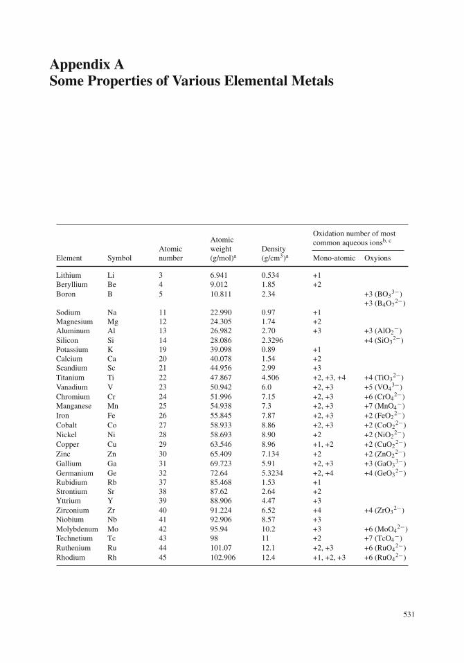
Appendix ASome Properties of Various Elemental Metals

Oxidation number of mostcommon aqueous ionsb, c

Element SymbolAtomicnumber

Atomicweight(g/mol)a

Density(g/cm3)a Mono-atomic Oxyions

Lithium Li 3 6.941 0.534 +1Beryllium Be 4 9.012 1.85 +2Boron B 5 10.811 2.34 +3 (BO3

3−)+3 (B4O7

2−)Sodium Na 11 22.990 0.97 +1Magnesium Mg 12 24.305 1.74 +2Aluminum Al 13 26.982 2.70 +3 +3 (AlO2

−)Silicon Si 14 28.086 2.3296 +4 (SiO3

2−)Potassium K 19 39.098 0.89 +1Calcium Ca 20 40.078 1.54 +2Scandium Sc 21 44.956 2.99 +3Titanium Ti 22 47.867 4.506 +2, +3, +4 +4 (TiO3

2−)Vanadium V 23 50.942 6.0 +2, +3 +5 (VO4

3−)Chromium Cr 24 51.996 7.15 +2, +3 +6 (CrO4

2−)Manganese Mn 25 54.938 7.3 +2, +3 +7 (MnO4

−)Iron Fe 26 55.845 7.87 +2, +3 +2 (FeO2

2−)Cobalt Co 27 58.933 8.86 +2, +3 +2 (CoO2

2−)Nickel Ni 28 58.693 8.90 +2 +2 (NiO2

2−)Copper Cu 29 63.546 8.96 +1, +2 +2 (CuO2

2−)Zinc Zn 30 65.409 7.134 +2 +2 (ZnO2

2−)Gallium Ga 31 69.723 5.91 +2, +3 +3 (GaO3

3−)Germanium Ge 32 72.64 5.3234 +2, +4 +4 (GeO3

2−)Rubidium Rb 37 85.468 1.53 +1Strontium Sr 38 87.62 2.64 +2Yttrium Y 39 88.906 4.47 +3Zirconium Zr 40 91.224 6.52 +4 +4 (ZrO3

2−)Niobium Nb 41 92.906 8.57 +3Molybdenum Mo 42 95.94 10.2 +3 +6 (MoO4

2−)Technetium Tc 43 98 11 +2 +7 (TcO4

−)Ruthenium Ru 44 101.07 12.1 +2, +3 +6 (RuO4

2−)Rhodium Rh 45 102.906 12.4 +1, +2, +3 +6 (RuO4

2−)

531

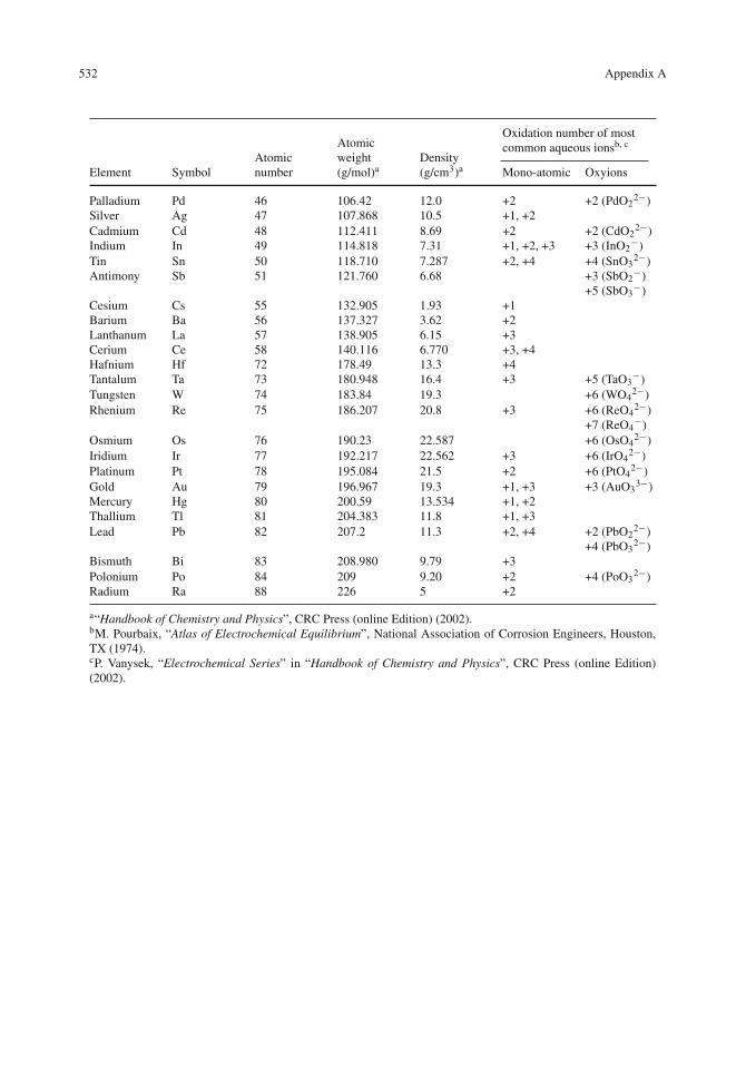
532 Appendix A

Oxidation number of mostcommon aqueous ionsb, c

Element SymbolAtomicnumber

Atomicweight(g/mol)a

Density(g/cm3)a Mono-atomic Oxyions

Palladium Pd 46 106.42 12.0 +2 +2 (PdO22−)

Silver Ag 47 107.868 10.5 +1, +2Cadmium Cd 48 112.411 8.69 +2 +2 (CdO2

2−)Indium In 49 114.818 7.31 +1, +2, +3 +3 (InO2

−)Tin Sn 50 118.710 7.287 +2, +4 +4 (SnO3

2−)Antimony Sb 51 121.760 6.68 +3 (SbO2

−)+5 (SbO3

−)Cesium Cs 55 132.905 1.93 +1Barium Ba 56 137.327 3.62 +2Lanthanum La 57 138.905 6.15 +3Cerium Ce 58 140.116 6.770 +3, +4Hafnium Hf 72 178.49 13.3 +4Tantalum Ta 73 180.948 16.4 +3 +5 (TaO3

−)Tungsten W 74 183.84 19.3 +6 (WO4

2−)Rhenium Re 75 186.207 20.8 +3 +6 (ReO4

2−)+7 (ReO4

−)Osmium Os 76 190.23 22.587 +6 (OsO4

2−)Iridium Ir 77 192.217 22.562 +3 +6 (IrO4

2−)Platinum Pt 78 195.084 21.5 +2 +6 (PtO4

2−)Gold Au 79 196.967 19.3 +1, +3 +3 (AuO3

3−)Mercury Hg 80 200.59 13.534 +1, +2Thallium Tl 81 204.383 11.8 +1, +3Lead Pb 82 207.2 11.3 +2, +4 +2 (PbO2

2−)+4 (PbO3

2−)Bismuth Bi 83 208.980 9.79 +3Polonium Po 84 209 9.20 +2 +4 (PoO3

2−)Radium Ra 88 226 5 +2

a“Handbook of Chemistry and Physics”, CRC Press (online Edition) (2002).bM. Pourbaix, “Atlas of Electrochemical Equilibrium”, National Association of Corrosion Engineers, Houston,TX (1974).cP. Vanysek, “Electrochemical Series” in “Handbook of Chemistry and Physics”, CRC Press (online Edition)(2002).

Appendix BThermodynamic Relationships for Use in ConstructingPourbaix Diagrams at High Temperatures

Consider the thermodynamic cycle shown in Fig. 6.19. At constant pressure:

Creactp (T − 298)+ �HT + Cprod

p (298− T)−�H298 = 0 (B1)

where Cpprodand Cp

react refer to the heat capacities at constant pressure of products and reactants,respectively. Thus,

�HT −�H298 = (Cprodp − Creact

p ) (T − 298) (B2)

or:

�HT −�H298 = �Cp (T− 298) (B3)

where �Cp= Cpprod − Cp

react. When the products and reactants are in their standard states, thenEq. (B3) becomes:

�H0T −�H0

298 = �C0p (T − 298) (B4)

or:

�H0T −�H0

298 =∫ T

298d(�H) =

∫ T

298�C0

pdT) (B5)

Because dS = dH/T at constant pressure,

�S0T −�S0

298 =∫ T

298

d(�H)

T=∫ T

298�C0

p d lnT) (B6)

Then

�G0T = �H0

T − T �S0T (B7)

and

�G0298 = �H0

298 − 298 �S0298 (B8)

533

534 Appendix B

combine to give:

�G0T −�G0

298 = (�H0T −�H0

298)− T(�S0T −�S0

298)− (�T)�S0298) (B9)

where �T = T − 298. Use of Eqs. (B5) and (B6) in Eq. (B9) gives the result:

�G0T = �G0

298 +∫ T

298�C0

P dT − T∫ T

298�C0

P d lnT − (�T)�S0298 (B10)

Equation (B10) is the expression for relating the standard free energy change at some elevatedtemperature T to the standard free energy change at 25◦C. Equation (B10) is the same as Eq. (30) inChapter 6. The heat capacities required in Eq. (B10) are either measured or estimated. Ionic entropiesare usually estimated by the empirical correlation method of Criss and Cobble [B1, B2] which relatesentropies at elevated temperatures to entropies at 298 K.

References

B1. C. M. Criss and J. W. Cobble., J. Am. Chem. Soc., 86, 5385 (1964).B2. J. W. Cobble, J. Am. Chem. Soc., 86, 5394 (1964).

Appendix CRelationship Between the Rate Constant and theActivation Energy for a Chemical Reaction

For the general reaction

A+B→ [AB] �= → products (C1)

where [AB] �=is the activated complex; see Fig. 7.14. The rate of the reaction depends on theconcentration of the activated complex and its rate of passage over the energy barrier; That is,

rate of reaction =(

concentrationof complex

)×(

rate of passageover energy barrier

)(C2)

When the activated complex is poised at the top of the energy barrier, its vibrational energy (hν) isjust equal to the thermal energy (kT). That is, hν = kT, where h is Planck’s contant, ν is the frequencyof vibration of the complex, and k is Boltzmann′s constant. Thus, ν = (kT/h) is the rate of passageof activated complexes over the energy barrier. Then, Eq. (C2) becomes

rate= [AB�=]kT

h(C3)

The equilibrium constant for the formation of the activated complex is

K �= = [AB�=]

[A][B](C4)

or

[AB �=] = K�=[A][B] (C5)

Also, �G�= = −RT ln K�= gives

K �= = e−�G�=/RT (C6)

Use of Eqs. (C5) and (C6) in Eq. (C3) gives

rate= [A][B]kT

he−�G�=/RT (C7)

But from classical kinetics,

535

536 Appendix C

rate= (rate constant) [A] [B] (C8)

Comparison of Eqs. (C7) and (C8) gives the result

rate constant = kT

he−�G�=/RT (C9)

which is the same as Eq. (6) in Chapter 7.

Appendix DRandom Walks in Two Dimensions

We want to calculate the root mean square distance√

< d2 > which a particle can move after Ntwo-dimensional steps. Suppose that after N−1 jumps, an atom or ion has the co-ordinates xN−1 andyN−1, as shown in Fig. D.1. As described in Chapter 8, let the jump distance be l units and supposethat the particle can jump in any of the eight discrete directions shown in Fig. D.2.

yN–1

xN–1

dN–1

(xN, yN)

(xN–1, yN–1)

Fig. D.1 A particle jumps from a given site to a new site one jump distance in the North direction

N

NE

E

SE

S

NW

SW

W

Fig. D.2 Diagram showing the possible jump directions considered in this example of a two-dimensional walk

537

538 Appendix D

Suppose that the particle jumps from co-ordinates (xN−1, yN−1) in the north direction (N), asshown in Fig. D.1. Then,

xN = xN−1 (D1)

and

yN = yN−1 + l (D2)

Squaring both sides of these two equations gives

X2N = X2

N−1 (D3)

and

Y2N = Y2

N−1 + 2 l yN−1 + l2 (D4)

Adding Eqs. (D3) and (D4) gives

x2N + y2

N = x2N−1 + y2

N−1 + 2lyN−1 + l2 (D5)

Equation (D5) can be written as

d2N = d2

N−1 + w2 (D6)

where

d2N−1 = x2

N−1 + y2N−1 (D7)

and

w2 = 2 l yN−1 + l2 (D8)

Instead of jumping from co-ordinates (xN−1, yN−1) in the north direction (N), suppose thatthe particle jumps in the northeast direction (NE). Then, from simple geometry, as shown inFig. D.3:

xN = xN−1 + l√2

(D9)

yN = yN−1 + l√2

(D10)

Squaring both sides in Eqs. (D9) and (D10) and adding gives

x2N + y2

N = x2N−1 + y2

N−1 +2 l√

2(xN−1 + yN−1)+ l2 (D11)

which again has the form of Eq. (D6), except now that

Appendix D 539

xN–1

yN–1

dN–1

(xN, yN)

(xN–1, yN–1)

/

2

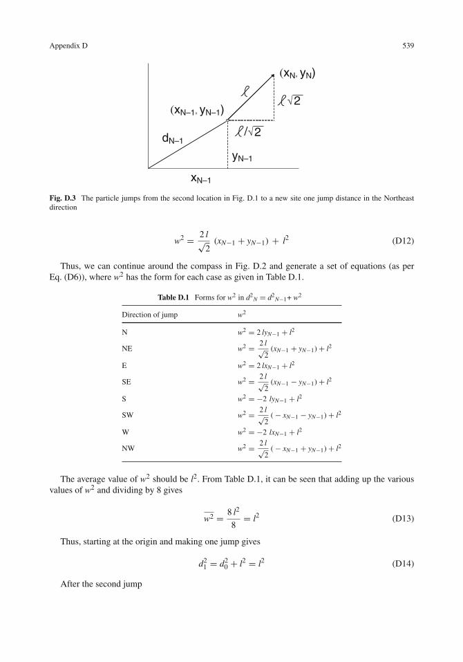
2

Fig. D.3 The particle jumps from the second location in Fig. D.1 to a new site one jump distance in the Northeastdirection

w2 = 2 l√2

(xN−1 + yN−1) + l2 (D12)

Thus, we can continue around the compass in Fig. D.2 and generate a set of equations (as perEq. (D6)), where w2 has the form for each case as given in Table D.1.

Table D.1 Forms for w2 in d2N = d2

N−1+ w2

Direction of jump w2

N w2 = 2 lyN−1 + l2

NE w2 = 2 l√2

(xN−1 + yN−1)+ l2

E w2 = 2 lxN−1 + l2

SE w2 = 2 l√2

(xN−1 − yN−1)+ l2

S w2 = −2 lyN−1 + l2

SW w2 = 2 l√2

(− xN−1 − yN−1)+ l2

W w2 = −2 lxN−1 + l2

NW w2 = 2 l√2

(− xN−1 + yN−1)+ l2

The average value of w2 should be l2. From Table D.1, it can be seen that adding up the variousvalues of w2 and dividing by 8 gives

w2 = 8 l2

8= l2 (D13)

Thus, starting at the origin and making one jump gives

d21 = d2

0 + l2 = l2 (D14)

After the second jump

540 Appendix D

d22 = d2

1 + l2 = 2 l2 (D15)

After the third jump

d23 = d2

2 + l2 = 3 l2 (D16)

Thus, in general,

d2N = Nl2 (D17)

or, the expected root-mean square value of d is

< d2 >= Nl2 (D18)

which is Eq. (5) in Chapter 8. Thus,

√< d2 > =

√Nl2 (D19)

It can be seen that if the jump direction is considered for a larger number of jump directions thatin turn approach a continuum, the result will be the same as in Eq. (D19).

Appendix EUhlig’s Explanation for the Flade Potential on Iron

Uhlig assumed that the following surface reaction was responsible for the passivation of iron:

Fe(s)+ 3H2O (1)→ Fe(O2 ·O)ads + 6H+(aq)+ 6e− (E1)

where Fe(O2·O)ads refers to the chemisorbed monolayer with a second layer of adsorbed O2molecules. The approach is to calculate the standard free energy change �G0 for Eq. (E1), andthen to get E0 from �G0 = −nFE0. The standard free energy change for Eq. (E1) is

�G0 = μ0 (Fe(O2 ·O)ads)+ 6μ0(H+(aq))− μ0((Fe(s))− 3μ0((H2O(1)) (E2)

Recall that μ0(H+(aq)) = 0 and μ0((Fe(s)) = 0. The value for μ0((H2O (l)) has been tabu-lated, but the value for μ0(Fe(O2.O)ads) is not available and must be calculated. Uhlig calculatedμ0(Fe(O2.O)ads) by considering the following surface reaction:

Fe (s)+ 3

2O2 → Fe (O2 ·O)ads (E3)

Uhlig then used

�G0S = �H0

S − T�S0S (E4)

where the subscripts refer to the surface reaction in Eq. (E3). With experimental data reported inthe surface chemistry literature for the heat of adsorption �Hs

0 and entropy of adsorption �Ss0 of

oxygen on iron, Eq. (E4) gives

�G0S =

(−75,000 cal

mol O2

)(3

2mol O2

)− 298◦

( −46.2 cal

deg mol O2

) (3

2mol O2

)(E5)

or, �Gs0 =− 91,848 cal per mole of Fe(O2·O)ads. This is also the value for μ0(Fe(O2.O)ads) because

Eq. (E3) involves the formation of Fe(O2·O)ads from its elements.Use of ΔGs

0 = − 91,848 cal for Fe(O2.O)ads in Eq. (E2) along with the value of−56,690 cal/mole for liquid water gives

�G0 = (1 mol Fe(O2 ·O)ads)

(−91,848 cal

mol

)− (3 mol H2O)

(−56,690 cal

mol

)

or, �G0 = 78,222 cal mol in Eq. (E1). Then,

541

542 Appendix E

�G0 = −nFE0 (E6)

gives

(78,222 cal)

(4.184 J

cal

)= −(6 equiv)

(96,500 coul

equiv

)E0 (E7)

or, E0 = − 0.57 V vs. SHE. But this value is for the oxidation reaction and the standard electrodepotential is for the reduction reaction, so that E0 = + 0.57 V vs. SHE. This value is in good agreementwith the Flade potential of +0.58 V for Franck’s data for iron in sulfuric acid.

Appendix FCalculation of the Randic Index X(G) for the Passive Filmon Fe–Cr Alloys

From Chapter 9, we begin with a hexagonal graph of Cr2O3 which contains Fe3+ ions substitutedfor some Cr3+ ions to form a mixed oxide, xFe2O3·(1−x) Cr2O3. The original hexagonal graph G0for Cr2O3 contains N vertices (Cr3+ ions) and (3/2) N edges (O2− ions). In the new graph G for themixed oxide D edges have been deleted one Fe3+ substituted per edge deletion. From Eq. (18) inChapter 9:

D

N= x

1− x(F1)

where x is the mole fraction of Fe2O3 in the mixed oxide.To calculate X(G), we would need to know which edges have been deleted from G0. However,

the process of edge deletion is random, so we follow the procedure used by Meghirditchian [F1] inanalyzing the network of a silica glass. For X(G), we use its expected value E[X(G)] given by

E[X(G)] =∑

i,j

(ij)−0.5E[A(G)ij ] (F2)

where A(G)ij is the number of edges in G connecting vertices of degrees i and j. We calculate the

expected value of E[A(G)ij ] following Meghirditchian [F1].

Edge deletion in the hexagonal network G0 can be treated by considering two adjacent verticesk and l in G0 and the connecting edge (kl), as shown in Fig. F.1. Suppose that after edge deletion,the edge (kl) remains undeleted, but the degrees of vertices k and l become i and j, as also shown inFig. F.1. To do this, we

(1) delete (3 − i) edges incident with the vertex k,(2) delete (3 − j) edges incident with vertex l, and(3) delete (D − 6 + i + j) edges from the remaining (3/2)N − 5 edges (See Table F.1).

k l i j

Fig. F.1 Edge deletion in a hexagonal network. After edge deletion, the vertices of degree k and l become i and j(shown here for the case where i and j are both two)

543

544 Appendix F

Table F.1 Edge deletion in a hexagonal array

Type edge Number of edges

Degree of vertex after edge deletion Possibilities

Number edges deleted

Ways to delete edges

kl 1 ---- ---- ---- ----

Incident with k

Incident with l

k

2 i i = 2 3 - i 2

i -1

i -1

j -1

i = 1 3 - i 2

l

2 j j = 2 3 - j 2

2

j -1

j = 1 3 - j

Remaining edges

32

N – 5 D - 6 + i + j

D - 6 + i + j

32

N - 5

The probability Pij of this occurrence is [F1, F2]

Pij =

(2

i− 1

)(2

j− 1

)( 3

2N − 5

D− 6+ i+ j

)

( 3

2N

D

) (F3)

Recall that(

ab

)= a!

b! (a− b)!From the properties of factorial numbers and for large N and D, Eq. (F3) becomes (after some

algebra)

References 545

Pij =

(2

i− 1

)(2

j− 1

)⎛⎜⎝3

2N−D

D

⎞⎟⎠

i+j−1

⎛⎜⎝

3

2N

D

⎞⎟⎠

5(F4)

which is the probability of any single edge (kl) in G0 becoming an edge of G joining vertices ofdegrees i and j. Then the expected value for the total number of edges in G joining vertices ofdegrees i and j is

E[A(G)ij ] = A(G0)Pij (F5)

where A(G0) is the number of edges in G. Thus

E[X(G)] = A(G0)3∑

j=1

3∑i=1

(ij)−0.5Pij (F6)

or

E[X(G)] = A(G0)3∑

j=i

3∑i=1

(ij)−0.5αijPij (F7)

where

αij ={

2 if i �=j1 if i = j

Use of Eqs. (F1) and (F4) in Eq. (F7) with A(G0) = (3/2)N gives

E[X(G)] =

(1

3

)5

N

(1− x)5(3− 5x) {24 x4 + 24

√2 x3(3− 5x)+ 4(

√3 + 3) x2 (3− 5x)2

+2√

6 × (3− 5x) 3 + 12 (3− 5x)4

}(F8)

References

F1. J. J. Meghirditchian, J. Am. Chem. Soc., 113, 395 (1991).F2. E. McCafferty, Electrochem. and Solid State Lett. 3, 28 (2000).

Appendix GAcid Dissociation Constants pKa of Bases and the Base Strength

Organic bases are protonated in acid solutions. For a secondary amine, for instance,

R2NH+ � R2N+H+ (G1)

where R2N denotes the depronated amine and R2NH+ its conjugate acid, with R referring to anorganic substituent. (If one of the R′s is an H atom, then the amine is a primary amine). The aciddissociation constant for Eq. (G1) is

Ka = [R2N] [H+]

[R2NH+](G2)

and

pKa = log1

Ka(G3)

The stronger the conjugate acid, the greater its tendency to produce protons. Thus, the strongerthe acid, the larger the ratio [R2N]/[R2NH+], and the larger the value of Ka. Large values of Kacorrespond to small values of pKa.

Thus, the smaller the pKa, the greater the acid strength. Conversely, the greater the pKa, thestronger base and greater the tendency to donate electrons.

547

Appendix HThe Langmuir Adsorption Isotherm

Suppose that a species A adsorbs from the aqueous phase onto a metal surface

A (aqueous)k1�

k−1A (adsorbed) (H1)

where k1 and k−1 refer to the rate constants in the forward (adsorption) and reverse (desorption)directions.

The process is represented by the free energy diagram in Fig. H.1(also see Chapter 7). In Fig. H.1,�G�=1 is the height of the free energy barrier in the forward direction, �G�=−1 is the correspondingheight in the reverse direction, and �Gads is the change in free energy due to adsorption of thespecies A.

A (adsorbed)

A (liquid)

ΔG1≠

ΔG-1≠

ΔGads

Extent of reaction

Free

ene

rgy

Fig. H.1 Free energy diagram for the adsorption of a species A from the aqueous phase onto a metal surface. �G �=1 is

the height of the free energy barrier in the forward direction, �G�=−1 is the corresponding height in the reverse direction,and �Gads is the change in free energy due to adsorption of the species A

The process of adsorption requires a vacant site on the metal surface (i.e., a site not already occu-pied by an adsorbed molecule or ion). From absolute reaction rate theory, as discussed in Chapter 7,the rate of adsorption (the forward direction) is

549

550 Appendix H

rate forward = k1 (1− θ ) Ce−�G�=−1/RT (H2)

where θ is the surface coverage of the adsorbed species and C is the concentration of species A inthe liquid phase. The rate of desorption (the reverse direction) is given by

rate reverse = k−1θe−�G�=−1/RT (H3)

At equilibrium the two rates are equal so that

k−1 θ e− �G�=−1/RT = k1 (1− θ ) Ce− �G�=−1/RT (H4)

Thus,

θ

1− θ= k1

k1Ce (�G�=−1−�G�=1 )/RT (H5)

But from Fig. H.1,

�G�=−1 −�G�=1 = �Gads (H6)

Use of Eq. (H6) in Eq. (H5) gives

θ

1− θ= k1

k−1e �Gads/RTC (H7)

Then we can write �Gads = �Hads − T �Sads, so that Eq. (H7) becomes

θ

1− θ= k1

k−1e−�Sads/Re �Hads/RTC (H8)

or

θ

1− θ= K1 e�Hads/RTC (H9)

where e−�Sads/R has been incorporated into the constant K1.In the Langmuir model, the metal surface is assumed to be homogeneous everywhere. In addition,

it is assumed that there are no lateral interactions between adsorbed molecules. (If there were lateralinteractions, then the heat of adsorption would vary with the surface coverage θ .) Thus, �Hads isindependent of the surface coverage θ . Then Eq. (H9) becomes

θ

1− θ= KC (H10)

where

K = K1 e�Hads/RT (H11)

Equation (H10) is the same as Eq. (7) in Chapter 12.

Appendix IThe Temkin Adsorption Isotherm

The Temkin adsorption isotherm removes the restriction in the Langmuir model that the heatof adsorption is independent of surface coverage θ . The Langmuir adsorption isotherm can bewritten as

θ

1− θ= K1 e�Hads/RT C (I1)

where the terms have the same meaning as in Eq. (H9).In the Temkin model, the heat of adsorption is assumed to decrease linearly with surface coverage

θ ; that is

�Hads = �H0ads − r θ (I2)

where �Hads0 is the initial heat of adsorption (at near-zero coverages) and r is the Temkin parameter.

Insertion of Eq. (I2) into Eq. (I1) gives

θ

1− θ= K1 e�H0/RT e−r θ/RT C (I3)

or

θ

1− θ= K′ e−r θ/RT C (I4)

where

K′ = K1 e�H0/RT (I5)

Taking natural logarithms in Eq. (I4) gives

ln

(θ

1− θ

)+ rθ

RT= ln K′ + ln C (I6)

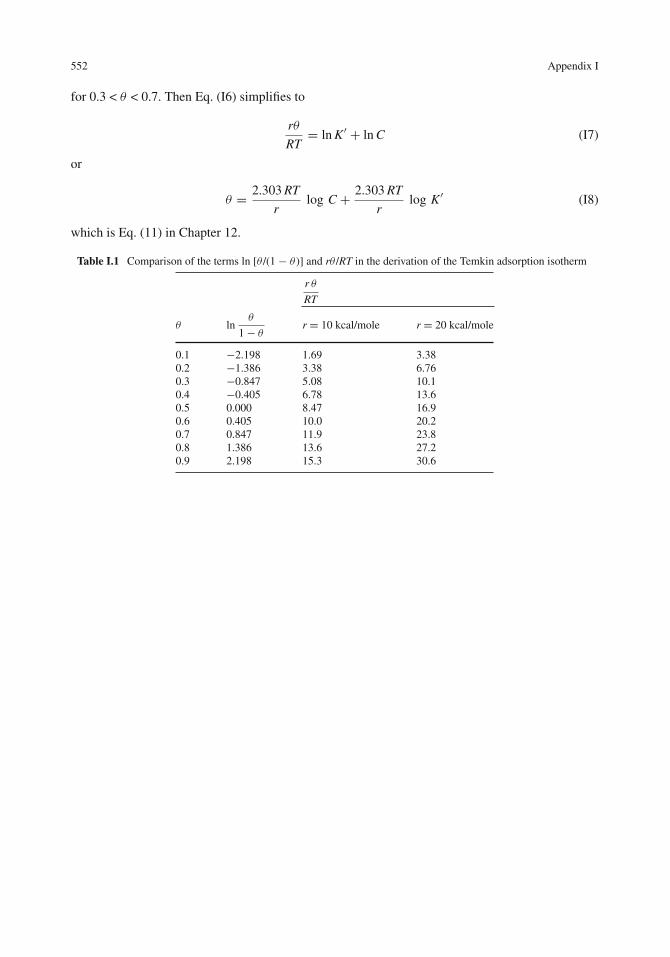
Next we compare the terms ln [θ /(1 − θ )] and rθ /RT. This is done in Table I.1 for typical valuesof r of 10−20 kcal/mol. As seen in Table I.1,

ln

(θ

1− θ

)<<

rθ

RT

551

552 Appendix I

for 0.3 < θ < 0.7. Then Eq. (I6) simplifies to

rθ

RT= ln K′ + ln C (I7)

or

θ = 2.303 RT

rlog C + 2.303 RT

rlog K′ (I8)

which is Eq. (11) in Chapter 12.

Table I.1 Comparison of the terms ln [θ /(1 − θ)] and rθ /RT in the derivation of the Temkin adsorption isotherm

r θ

RT

θ lnθ

1− θr = 10 kcal/mole r = 20 kcal/mole

0.1 −2.198 1.69 3.380.2 −1.386 3.38 6.760.3 −0.847 5.08 10.10.4 −0.405 6.78 13.60.5 0.000 8.47 16.90.6 0.405 10.0 20.20.7 0.847 11.9 23.80.8 1.386 13.6 27.20.9 2.198 15.3 30.6

Appendix JThe Temkin Adsorption Isotherm for a Charged Interface

If a molecule or ion adsorbs at a charged interface in the presence of an electrode potential,

A (aqueous)k1�

k−1A (adsorbed)

then the process is represented by the free energy diagram in Fig. J.1, where the solid lines inFig. J.1 apply to the open-circuit potential E0.

A (adsorbed)

A (liquid)

ΔG1≠

ΔG-1≠

ΔGads

Extent of reaction

Fre

e en

ergy

αzF(E - E0)

(1 - α)zF(E - E0)

Fig. J.1 Free energy diagram for the adsorption of a species A from the aqueous phase onto a metal surface in thepresence of an electrode potential. The solid lines refer to the open-circuit potential E0, and the dotted lines to apolarized potential E. �G�=1 is the height of the free energy barrier in the forward direction at potential E0, �G�=−1is the corresponding height in the reverse direction at potential E0, and �Gads is the change in free energy due toadsorption of the species A at potential E0

Suppose that the adsorbed species has a negative charge, and that the electrode potential ischanged from the open-circuit potential E0 to a more positive potential E. Then the height of the freeenergy barrier will be decreased for adsorption (the forward direction) and increased for desorption(the reverse direction), as shown by the dotted lines in Fig. J.1.

553

554 Appendix J

The rate of adsorption in the forward direction at the open-circuit potential E0 is

rate forward = k1 (1− θ )[A] e−�G1�=/RT (J1)

(see Eq. (H2) in Appendix H). Under the new applied potential E, the rate of adsorption in theforward direction is

rate forward = k1 (1− θ ) [A] e−[�G�=−αzF(E−E0)

]/RT (J2)

where z is the charge on the adsorbing species, α is the symmetry factor, and αZF(E− E0) representsthe coulombic interaction of the charge with the electric field. (If the decrease in the free energybarrier in the forward direction is equal to the increase in the free energy barrier in the reversedirection, then α = 0.5.)

Similarly, the rate of desorption in the reverse direction under potential E is

rate reverse = k−1 θ e−[�G�=−1+ (1−α)zF(E−E0)

]/RT

(J3)

At equilibrium under the potential E, the rate in the forward direction is equal to the rate in thereverse direction, or

k−1 θ e−[�G�=−1+ (1−α)zF(E−E0)

]/RT = k1 (1− θ ) [A] e

−[�G�=1 −αZF(E− E0)

]/RT

(J4)

Thus,

θ

1− θ= k1

k−1[A] e(�G�=−1−�G�=1 )/RT e−zFE0/RT ezFE/RT (J5)

As in Appendix H,

�G�=−1 −�G�=−1 = �Gads (J6)

and writing �Gads = �Hads − T �Sads gives

θ

1− θ= k1

k−1[A] e�Hads/RTe−�Sads/R e−zFEo/RT ezFE/RT (J7)

As in Appendix I, we write

�Hads = �H0ads − r θ (J8)

where �Hads0 is the initial heat of adsorption (at near-zero coverages) and r is the Temkin parameter.

Then

θ

1− θ= k1

k−1[A] e�H0

ads/RTe−rθ/RT e−�Sads/R e−ZFEo/RT ezFE/RT (J9)

θ

1− θ= K2 [A] e−rθ/RT ezFE/RT (J10)

Appendix J 555

where

K2 = k1

k−1e�H0

ads/RTe−�Sads/R e−zF E0/RT (J11)

Equation (J10) has a form similar to that of Eq. (I4) in Appendix I, and the remainder of thetreatment is similar to that in Appendix I. Taking logarithms in Eq. (J10) gives

ln

(θ

1− θ

)+ rθ

RT= ln K2 + ln [A]+ zFE

RT(J12)

As shown in Appendix I,

ln

(θ

1− θ

)<<

rθ

RT

for 0.3 < θ < 0.7. Then Eq. (J12) becomes

θ = 2.303 RT

rlog [A]+ 2.303 RT

rlog K2 + zFE

r(J13)

which is Eq. (18) in Chapter 12.

Appendix KEffect of Coating Thickness on the Transmission Rateof a Molecule Permeating Through a Free-StandingOrganic Coating

Consider the case where the exterior of the coating is in contact with concentration C0 of permeatingmolecule. The concentration profiles with time within an organic coating of thickness L1 are givenin Fig. K.1. The concentration of permeating molecule at the underside boundary of the organic filmis zero because the permeating molecules exit the film at that distance.

Distance from surface

t1 t2t3

Concentrationof permeant in coating

Distance from surface

t1 t2t3 t4

L1

L2

t5

C0

C0

Concentrationof permeant in coating

Fig. K.1 Concentration profiles (at different times) for a permeating molecule in free-standing organic films ofthickness L1 (top) and L2 (bottom)

From Ficks first law of diffusion, the transmission rate J1 of the permeating molecule in thecoating of thickness L1 is

J1 = −DdC

dx(K1)

or

J1 = −D

(0− C0

L1

)(K2)

557

558 Appendix K

For a second coating of identical material but of a different thickness L2,

J2 = −D

(0− C0

L2

)(K3)

Equations (K2) and (K3) combine to give:

J2

J1= L1

L2(K4)

Appendix LThe Impedance for a Capacitor

The voltage across a capacitor C is

E(t) = 1

CQ(t) (L1)

where Q(t) is the charge given by

Q(t) = I(t)t (L2)

Use of Eq. (L2) in Eq. (L1) gives

E(t) = 1

CI(t)t (L3)

so that

d E(t)

d t= 1

CI(t) (L4)

and

I(t) = Cd E(t)

d t(L5)

The impedance is given by

ZC = E(t)

I(t)= E(t)

Cd E(t)

dt

(L6)

The voltage E(t) is given by Eq. (6) in Chapter 14, that is

E = E0 ejωt (L7)

Use of Eq. (L7) in Eq. (L6) gives

ZC = E(t)

I(t)= E0ejωt

CjωEjωt0

(L8)

or

ZC = 1

jωC(L9)

Reference

L1. G. H. Hostetter, “Fundamentals of Network Analysis”, p. 162, Harper & Row, New York, NY (1980).

559

Appendix MUse of L’Hospital’s Rule to Evaluate |Z| for theMetal/Solution Interface for Large Values of AngularFrequency ω

For the model of the electrical double layer shown in Fig. 14.4, we have

|Z| =⎧⎨⎩(

RS + Rp

1+ ω2R2p C2

dl

)2

+(

ωR2p Cdl

1+ ω2R2p C2

dl

)2⎫⎬⎭

1/2

(M1)

which is Eq. (24) in Chapter 14. For ω → ∞, the first term in the parentheses on the right-handside of Eq. (M1) approaches (Rs)2, but we need to apply L’Hospital’s rule to the second term on theright-hand side of Eq. (M1). Thus,

limω→∞

(ω R2

p Cdl

1+ ω2R2p C2

dl

)= lim

ω→∞

⎛⎜⎝

d

dω

(ωR2

p Cdl

)d

dω

(1 + ω2R2

p C2dl

)⎞⎟⎠ (M2)

limω→∞

(ω R2

p Cdl

1+ ω2R2p C2

dl

)= lim

ω→∞

(R2

p Cdl

2ωR2p Cdl

)(M3)

or

limω→∞

(ω R2

p Cdl

1+ ω2R2p C2

dl

)= 0 (M4)

Thus,

limω→∞ |Z| = |R

2S|1/2 = RS (M5)

561

Appendix NDerivation of the Arc Chord Equation for Cole−Cole plots

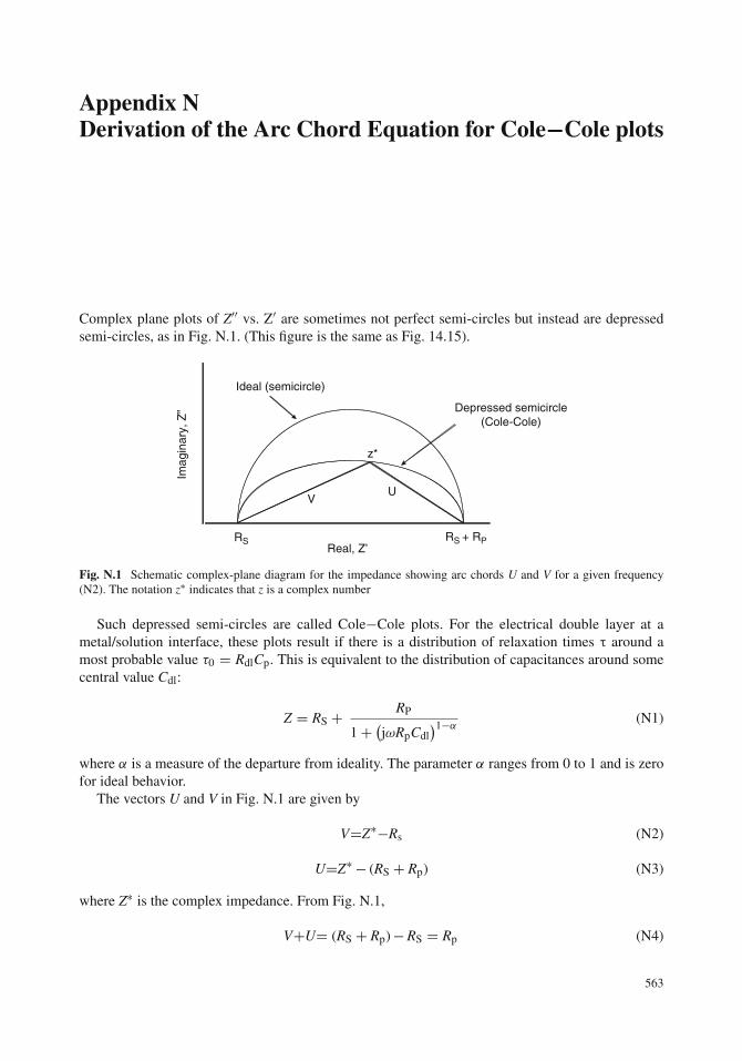
Complex plane plots of Z′′ vs. Z′ are sometimes not perfect semi-circles but instead are depressedsemi-circles, as in Fig. N.1. (This figure is the same as Fig. 14.15).

Depressed semicircle(Cole-Cole)

z*

VU

Imag

inar

y, Z

”

Real, Z’

Ideal (semicircle)

RS RS + RP

Fig. N.1 Schematic complex-plane diagram for the impedance showing arc chords U and V for a given frequency(N2). The notation z∗ indicates that z is a complex number

Such depressed semi-circles are called Cole−Cole plots. For the electrical double layer at ametal/solution interface, these plots result if there is a distribution of relaxation times τ around amost probable value τ0 = RdlCp. This is equivalent to the distribution of capacitances around somecentral value Cdl:

Z = RS + RP

1+ (jωRpCdl)1−α

(N1)

where α is a measure of the departure from ideality. The parameter α ranges from 0 to 1 and is zerofor ideal behavior.

The vectors U and V in Fig. N.1 are given by

V=Z∗−Rs (N2)

U=Z∗ − (RS + Rp) (N3)

where Z∗ is the complex impedance. From Fig. N.1,

V+U= (RS + Rp)−RS = Rp (N4)

563

564 Appendix N

Then Eq. (N1) becomes

V + U = V + U

1+ (jωRpCdl)1−α(N5)

or

V + V(jωRpCdl)1−α = V + U (N6)

so that

V

U= 1

(jωRpCdl)1−α(N7)

or

V

U= (jωRpCdl)

α−1 (N8)

Taking absolute values on each side

∣∣∣∣VU∣∣∣∣ = |j (α−1)

∣∣∣ (ωRpCdl)α−1 (N9)

Then use is made of the property that any complex number can be written in polar form:

z = a+ jb = r ejθ (N10)

For the special case where z = j,

j = 1·ej π2 (N11)

j(α−1) = e(j π2 )(α−1) (N12)

or

j(α−1) = cosπ

2(α − 1)+ j sin

π

2(α − 1) (N13)

With

| z| =√

a2 + b2 (N14)

∣∣∣j(α−1)∣∣∣ =

√cos2

[π2

(α − 1)]+ sin2

[π2

(α − 1)]= 1 (N15)

Use of this result in Eq. (N9) gives

∣∣∣∣VU∣∣∣∣ = (ωRpCdl)

α−1 (N16)

References 565

and

log

∣∣∣∣VU∣∣∣∣ = (α − 1) log ω + (α − 1) log (CdlRp) (N17)

which is the desired result.

References

N1. E. McCafferty, V. H. Pravdic, and A. C. Zettlemoyer, Trans. Faraday Soc., 66, 1720 (1970).N2. K. S. Cole and R. H. Cole, J. Chem. Phys., 9, 341 (1941).N3. E. McCafferty and J. V. McArdle, J. Electrochem. Soc., 142, 1447 (1995).

Appendix OLaplace’s Equation

The flux Ni of each dissolved species in an electrolyte arises from three effects. These are: (a)the motion of charged species in an electric field (migration), (b) diffusion due to a concentrationgradient, and (c) convection due to bulk motion of the fluid. These three contributions give [O1]

Ni = -zi μ i F Ci ∇φ - Di ∇ Ci + Ci v

migration diffusion convection (O1)

whereNi = ionic flux of species izi = charge of species iμi = mobility of species iF = Faraday’s constantCi = concentration of species iφ = electrostatic potentialDi = diffusion coefficient of species iv = fluid velocity∇ = differential operator (∂ /∂x + ∂ /∂y + ∂ /∂z)

The current density i is given by

i = F∑

i

ziNi (O2)

The material balance of each species is

∂Ci

∂t= −∇ Ni + Ri (O3)

where Ri is the rate of production of species i due to chemical reactions in the bulk of the electrolyte.If ions are not generated in the bulk, then Ri = 0.

The condition of electroneutrality in the solution is

∑i

zi Ci = 0 (O4)

567

568 Appendix O

Multiplying Eq. (O3) by zi gives

∂(ziCi)

∂t= −∇ ziNi (O5)

(with Ri = 0). Then, summing over all species gives

∂

∂t

∑i

zi Ci = −∇∑

i

ziNi (O6)

But from Eq. (04),∑

izi Ci = 0, so that Eq.(06) gives

∇∑

i

ziNi = 0 (O7)

Then, Eq. (O2) can be written as

∇i = ∇(

F∑

i

ziNi

)= F

∑i

ziNi (O8)

Using Eq. (O7) in Eq. (O8) gives

∇i = 0 (O9)

This result will be used below. Use of Eq. (O1) in Eq. (O2) gives

i = F∑

i

zi (−zi μiFCi∇φ − Di∇Ci + Civ)

or

i = −F2∇φ∑

i

z2i μiCi − F

∑i

zi Di∇Ci + Fv∑

i

ziCi (O10)

By virtue of electroneutrality, the last term is zero. If there are no concentration gradients in thebulk of the solution, ∇Ci = 0. Thus, Eq. (O10) becomes

i = −σ ∇φ (O11)

where σ is the electrolyte conductivity given by

σ = −F2∑

i

z2i μiCi (O12)

We can operate on Eq. (O11) as follows:

∇i = −σ ∇2φ (O13)

Reference 569

But ∇i = 0 by Eq. (O9), so that Eq. (O13) gives

∇2φ = 0 (O14)

which is Laplace’s equation.

Reference

O1. J. Newman, in “Advances in Electrochemistry and Electrochemical Engineering”, C. W. Tobias, Ed., Vol. 5,p. 87, Interscience Publishers, New York, NY (1967).

Index

AAbsolute reaction rate theory, 131–132, 136, 549AC circuit analysis, 430–431Acid–base properties of oxides, 477, 494–499, 511–512Acidic solutions and inhibitors, 360–379Acidification within crevices, 322Acidification within pits, 321–322Acid solutions and concentration polarization, 148,

177–178, 200–202Acid solutions, metals in, 146–148AC impedance

anodization, 446, 448–449corrosion inhibition, 370, 449effect of diffusion, 436–437experimental set-up, 370, 429–430, 441, 450organic coatings, 370, 422, 427, 441–446, 449surface treatment, 422, 427, 446–448, 449

Activation polarization, 127–146, 177–179, 202–203, 484

Active/passive transition, 168, 211–212, 237, 254–255,290–291, 503

Adhesion of organic coatings, 232, 412–416, 494Adsorption inhibitors, 359Adsorption theory of passivity, 217, 238Aging infrastructure, 3Aluminum, 1, 6, 8, 13, 21–23, 77–79, 96–101, 122–124,

209–211, 230–235, 280–283, 297–300, 305,334, 351, 373, 385, 397, 446–448, 496–499,501–505

Aluminum, corrosion rate vs. pH, 78, 101Anodic control, 158–159, 343Anodic dissolution and stress-corrosion cracking, 339,

343–345, 353Anodic polarization, 128–130, 136, 149, 159, 168–169,

171, 179, 193, 211–215, 237–238, 250, 254,274, 277–280, 288–289

Anodic protection, 105, 255–257, 357Anodic reactions, 15–16Anodization, 211, 232, 446–449Anodization and AC impedance, 446, 448–449Anodizing, 211, 233, 518Applications of mixed potential theory, 146–159Area effects, 83, 199, 274–275

BBase strength and inhibition, 365, 374Batteries, 517Beneficial aspects of corrosion, 6, 515–518Binary alloys, 111–112, 151, 216–218, 237–248,

252, 271Biological molecules as inhibitors, 382, 390Bockris–Devanathan–Muller model of the electrical

double layerinner Helmholtz plane, 42Bockris–Kelly mechanism, 478–481Bode plots, 434–441, 444–445, 447–448, 450Body implants, 2, 278, 315–316, 348Breakdown of organic coatings, 416

CCapacitance of electrical double layer,

441, 443Cathode area, 82–83, 154, 200, 309Cathodic control, 158–159, 192, 343, 488Cathodic delamination, 412–413, 419–422Cathodic polarization, 127–129, 137, 143, 148, 159,

171, 173, 179, 191, 193, 199, 200, 254, 258,266, 308, 337

Cathodic protection, 79–81, 105, 150–153, 197–199,209, 255–258, 276, 337, 346, 351–352, 404,412, 490

Cathodic protection in acids, 150, 153, 199, 255–256,337, 357, 412, 517

Cathodic reactions, 16–17, 19–21, 149, 156, 203secondary effects, 19–21

Cavitation, 13–14, 315, 317, 349–352, 354Cavitation corrosion, 14, 315, 349–352Challenges, 9–10, 422–423Chemical potential, 63–66, 71–72, 97, 100,

114, 209Chemisorption of inhibitors, 361–362Chloride and stress-corrosion cracking, 3, 9, 14, 26, 211,

263, 277, 301, 320, 336, 345, 382Chromate, 3, 9, 65, 71, 106, 109–110, 115, 158,

212–213, 229, 237, 255, 273, 276, 306, 357,360, 380–382, 405, 414, 446–448

Chromate replacements, 71, 381–382, 399Cole–Cole plots, 433, 438

571

572 Index

Concentration polarization, 127–131, 148, 162, 167,177–208

kinetics, 131, 177, 186–192limiting current density, 191, 193polarization curves, 139, 144, 149, 177, 279,

292, 362Conservation of materials, 1, 5–6, 9Copper, pitting of, 278Corrosion

beneficial aspects, 6, 515–518definition, 13, 16quotations about, 515

Corrosion fatigue, 7–9, 14, 315, 346–349, 354,387–389

Corrosion inhibition and AC impedance, 370,438–441, 449

Corrosion inhibitors, 4, 9, 109, 163, 173, 209, 276, 283,348, 352, 357–400, 414, 422

Corrosion rates, 24–25, 48, 78, 101, 111, 119, 150–151,154, 162, 164, 170, 196, 200, 209, 236–237,240, 255, 346, 375, 378–379

methods, 119–127Corrosion science vs. engineering, 8–9Corrosion testing of organic coatings, 419–423Corrosion of works of art, 6Cost of corrosion, 1, 4, 10Coupled reactions, 17–18, 19, 60Crevice corrosion, 27, 89, 211, 249, 263–277, 322, 357,

361, 382, 386–387, 412, 417, 483area effects, 83, 199, 274–275effect of temperature, 196–197, 294–296initiation, 26, 263–265, 272, 280, 300, 307, 320, 357local acidification, 321oxygen depletion, 186propagation, 269–272, 274, 286, 357protection against, 83–84, 263testing, 264, 272–274

Critical relative humidity, 18–20Current distribution, 130, 167, 306, 477, 486–487, 493

DDealloying, 27–28Defect nature of oxides, 463–472Detection of pits, 307Differential concentration cells, 84–89Differential oxygen cell, 86, 89, 264Diffusion, 111, 159, 177–208, 264, 266, 269, 273, 282,

290, 300, 302, 407–408, 412, 417, 419, 421,436–437, 449, 456–457, 459, 463, 464

Diffusion and AC impedance, 449Diffusion and high temperature oxidation, 456–457, 459,

463, 469, 471–473Diffusion layer, 188–189, 194, 206, 266,

269, 488Diffusion and random walks, 183–185Distribution

circular corrosion cells, 483–486

of current, 306, 483–489of potential, 307

Drinking water problems, 3–4, 71, 178, 357–358

EEffect of O2 concentration on corrosion, 193Effect of O2 pressure on high temperature oxidation,

453–457, 462, 466, 469, 472–474Effect of temperature on corrosion, 196–197, 294, 296,

338–339, 463Effect of temperature on oxidation, 463Effect of velocity on corrosion, 194–196Eight forms of corrosion, 27–28Einstein–Smoluchowski equation, 185Electrical double layer, 37, 39–44, 52, 129, 189,

370–372, 432, 441, 443, 556–557Bockris–Devanathan–Muller, 42capacitance and, 43, 370–372, 378, 398Guoy–Chapman layer, 42inner Helmholtz plane, 41–42, 44, 371outer Helmholtz plane, 42, 371Stern mode, 41–42

Electrochemical cells, 67, 73–92, 167–168, 489, 493on the same surface, 75–76

Electrode kinetics, 131–146, 186–192, 477–482Electrode potential, 43–53, 65–66, 68–70, 75–87, 90–92,

95–99, 102–106, 111–112, 114, 127–128,131, 134–141, 150, 179, 185, 189–191

factors affecting, 69–70measurement of, 52–53sign, 68–70standard, 45–48, 65–66, 68–69, 76, 115, 127, 139,

147, 185, 189–191, 216, 257, 541Electrolytes, 18, 21, 30, 33–35, 53, 169, 181, 185, 199,

206, 232, 269–270, 273–274, 290–291, 300,322, 330–332, 409, 484, 488–489

Electromotive force series, 46–48limitations of, 111–112

Electron configuration theory of binary alloys, 238–241,257–258

Electrostatic potential, 40–41, 44, 65, 483, 485, 560Ellingham diagrams, 454–455Erosion, 13–14, 27–28, 315–316, 321, 352–354Erosion–corrosion, 28, 354Evans diagrams, 143, 150, 152, 154, 157–158, 171,

190–192, 194, 196, 198, 200, 206, 267,269, 275

Evans water drop experiment, 88Exchange current density, 133, 138–139, 142–147, 150,

154–155, 254Experimental Pourbaix diagrams, 111, 291–293, 310Experimental techniques, 165–169, 423

FFaraday’s Law, 23–25, 150Fatigue, 2, 7, 9, 13–14, 315, 321, 329–330, 346–349,

351, 354, 387–389

Index 573

Fermi sea of electrons, 38–39Fick’s first law, 181–182, 187, 407, 467Filiform corrosion, 417–419Film-forming inhibitors, 359Film sequence theory of passivity, 215, 218Flade potential, 211–213, 216, 237, 239, 257, 541–542Fracture, 8–9, 13–14, 28, 234–235, 316, 318–320,

323–324, 335, 340–341, 343–347Fracture mechanics, 323–331, 334, 353Fracture-safe diagrams, 334, 353Fretting corrosion, 14, 315–316, 352–354

GGalvanic corrosion, 27, 57, 73–92, 154–156, 199,

483, 490protection against, 83–84

Galvanic series, 76–79, 83, 89–91, 150, 199, 207Gaseous oxidation, 453–475Graph theory of Fe–Cr alloys, 243–248Guoy–Chapman layer, 42

HHarsh environment, 1–2Hauffe rules of oxidation, 466–471Henry’s law, 180, 197, 208, 407Heusler mechanism, 480–481High temperature oxidation, 9, 235, 453–460, 462–463,

469, 471–473High temperature oxide films

defect nature, 463–464layers on pure iron, 233, 395properties of protective films, 210semiconductor nature, 465–466

Hydration of ions, 35, 38–39, 42, 229–230, 235, 285Hydrogen embrittlement, 21, 103, 321, 339,

342–346

IInhibition of crevice corrosion, 302, 386Inhibition of pitting, 382–387Inhibition of stress-corrosion cracking, 341, 361,

382–389Inhibitors

adsorption inhibitors, 359acidic solutions, 360, 363–368, 373, 375, 379base strength effects, 364–365, 374concentration effects, 128, 150crevice corrosion, 273, 276, 283, 294, 296, 302,

357–399film-forming inhibitors, 359localized corrosion, 25–28, 109, 111, 293, 361,

382–389molecular size effects, 373–376molecular structure effects, 373–376, 414neutral solutions, 109, 358passivating inhibitors, 359pitting, 9, 263–311, 387

precipitation inhibitors, 359stress-corrosion cracking, 357, 382

Interfaces, 33–55, 316, 349, 414, 428, 485Intergranular corrosion, 27–28, 335Ion implantation, 124–125, 301, 348, 477, 499–505,

509–510Iron

–chromium alloys, 237dissolution, 141, 150, 190, 192–194, 477–482

microstructure, effect of, 335, 351nail experiment, 30–31

Irreversible potentials, 139–140Isoelectric point of oxides, 416, 505

KKI, 319, 325–329, 333–334, 345, 353, 387, 479KIscc, 329–337, 345, 353, 387–389Kramer–Kronig transforms, 440

LLangmuir–Blodgett films, 393–396Laplace’s equation, 483, 485, 490–491Laser-surface alloying, 509Laser-surface melting, 512Levich equation, 202, 204Limiting diffusion current, 187–188, 192–194, 196, 199,

201–203, 206Linear polarization, 159–165, 199–200, 484Localized corrosion

crevice corrosion, 25–27, 111, 211, 249, 263inhibition of, 382–389pitting, 25, 27, 211, 235, 263, 277–297stress-corrosion cracking, 25–27, 211, 263, 315–316

Luggin–Haber capillary, 53–54, 130–131, 167–168

MMagnesium–graphite couple, 78Mechanical metallurgy, 318–319Mechanism of pit initiation, 283–286Mechanism of pit propagation, 286–288Mechanisms of stress-corrosion cracking, 346Metallic coatings

galvanized steel, 4, 13, 29, 80–81titanium, 82–83zinc–aluminum, 81

Metals-based society, 1Metal/solution interface, 16, 23, 33, 36–42, 44–45, 65,

227, 357, 371–372, 427, 431–441, 443, 449,496, 556

Metastable pits, 290–291Mixed control, 158–159Mixed potential theory, 140–144, 146–159Mo effect on pitting, 293–294Molecular structure and inhibition, 373–376, 414Monolayers, 225, 393–396, 410Multiple oxidation–reduction reactions, 156–158

574 Index

NNernst equation, 66–68, 75, 77, 85, 87, 97–101, 112,

139, 141, 189, 191, 216, 265, 399Noble metal alloying, 256Non-uniform oxide layers on iron in high temperature

oxidation, 472Nuclear waste disposal, 3Nyquist plots, 433

OOccluded corrosion cells, 300–306, 386Ohmic polarization, 127, 130–131, 484Organic coatings, 8, 10, 83, 209, 232, 357, 382, 403–424,

441–446, 449Organic coatings and AC impedance, 422, 427, 441,

444, 449Outer Helmholtz plane, 42, 371Overvoltage, 127, 136, 138–139, 142, 148, 150,

157–158, 161, 172, 178, 190–191, 202, 268,372, 488

Oxidation rate laws, 457–463Oxide film properties of Fe–Cr alloys, 241–242Oxide film theory of passivity, 218Oxygen reduction, 87, 177–178, 179, 186, 188, 191–194,

197, 199, 205–207, 264, 269, 274, 379, 423,472, 488, 527

Oxygen scavengers, 193

PPaint, 10, 78, 80, 357, 403–405, 407–408, 412, 417, 422Parabolic rate law, 459, 460–463Passivating inhibitors, 359Passive films

aluminum, 210–211, 217, 230, 233–235, 278, 283,285–286, 297–300

properties, 110, 210, 215, 217–218, 228–229,234–235, 241–242, 473, 494–499

structure, 219, 227, 229–230, 233, 235, 241, 353,359, 499

surface analysis, 253thickness, 210–211, 215, 217–218, 228, 230, 233,

235, 257, 285, 473Passivity, 9, 95–96, 101, 103–110, 209–259, 263, 278,

288, 290, 292–293, 305, 310alloying and, 509aluminum, 95–96, 101–103, 209–211, 217, 230–232,

283, 286, 297, 298–300, 305, 351, 384, 499bilayer model for iron, 224–227binary alloys, 112, 216–218, 237–238, 240–241,

243, 246, 529bipolar model, 229, 253definition, 210effect of Mo, 258electrochemical basis, 211–215Fe–Cr, 112, 217–218, 229, 237–243, 248, 250, 252,

289, 293, 331history, 210

hydrous model for iron, 227–228models for iron, 222, 224–230spinel defect model, 224–225, 229–230stainless steel, 9, 158, 214, 217, 228, 230, 234, 238,

248–253, 278–279, 283, 289–291, 294, 297,320, 331, 352, 508

theories, 215–218Percolation theory of Fe–Cr alloys, 242–243Permeation of Cl− into organic coatings, 411Permeation of H2O into organic coatings, 406–410Permeation of O2 into organic coatings, 410–411pH and stress-corrosion cracking, 338Physical degradation, 13–14Pilling–Bedworth ratio, 234–236, 472–473Pitting, 263–311, 382–386, 497–499

of aluminum, 283, 286, 297–300, 385, 499chloride ions, 9, 214, 235, 263, 277, 287, 291, 293,

297, 412, 499detection of, 306–308inhibition, 302, 357, 361, 382–397, 494local acidification, 321metastable, 290–291propagation, 263, 280, 283, 286–290, 298–299, 322,

357, 382protection against, 296–297, 529stainless steel, 9, 27, 214–215, 249, 278, 289–290,

294, 297, 320, 384, 497Pitting potential

effect of chloride, 282inhibition, 283

Polarization, 127–146, 159–169, 177–208curves, 136–138, 143, 147–151, 160, 165–169,

191–192, 197–205, 212–215, 236–238, 250,266, 268, 274, 279–280, 288

Potential difference, 33, 40–41, 43–45, 54Potential distribution, 418–419, 483–491, 511Potential of zero charge, 372–373Pourbaix diagrams

aluminum, 96, 234chromium, 106–107, 110copper, 111–112experimental, 57, 67, 95–116, 214–215, 233–234,

291–293, 301, 342–343iron, 103–106water, 95, 98, 101–103, 112, 114zinc, 103

Precipitation inhibitors, 360Properties of protective high temperature oxides,

473–474Protection against corrosion fatigue,

348–349Protection against pitting, 296–297Protection potential, 288–293

RRandom walks, 183–185Rate laws in oxidation, 457–463

Index 575

Reference electrodestable of, 50copper/copper sulfate, 50–51saturated calomel, 48, 50, 52, 70, 77in seawater, 49–50silver/silver chloride, 49standard hydrogen electrode, 48, 50

Relative electrode potential, 45–46Relaxation processes, 427–429Rotating disc electrode, 202–205Rotating ring disc electrode (RRDE), 205Rust, 5, 7, 13–14, 18, 60, 83, 88, 170, 205, 240, 249,

315–316, 422, 457, 474, 515–516

SSafety, 1–4, 515Scaling rules, 477, 489–493Scanning tunneling microscopy (STM), 219, 223–224,

229, 244Seawater corrosion, 78–79Self-assembled monolayers, 393–396Semiconductor nature of oxides, 465–466Sensitization, 27, 339Smart coatings, 423Solubility and diffusion, 179–185Solubility product, 22, 29, 71, 290, 360Solution/air interface, 33, 35–37Spontaneity, 47, 60, 399Stainless steels, 1, 6, 8–9, 14, 158, 217, 229, 249–253,

274, 289, 293–294, 320–321, 348, 352Stainless steels passivity, 249–253Standard hydrogen electrode (SHE), 45–48, 50–51, 54,

64–65, 77, 85, 96–98, 100Stern–Geary, 159–165, 199, 484Stern model of the electrical double layer, 41Strain, 235, 318–319, 325, 375–376Stress, 1, 3, 7–9, 14, 20, 70, 103, 211, 277, 300–303,

315–348, 361, 382, 387–389, 483Stress-corrosion cracking, 7–9, 14, 20, 25–27, 103,

211, 263, 277, 301, 305, 315–324, 330, 333,335–337, 345–346, 353–354

effect of Cl− concentration, 338–339, 384effect of electrode potential, 336–338, 340, 353effect of pH, 212, 338effect of temperature, 196–197, 338–339flaws and, 320–321, 382, 389initiation, 264–269mechanisms, 8–9, 230, 263, 286, 293, 300, 337, 339metallurgical effects, 335–336modes of, 322propagation, 26–27, 263, 320, 338, 357properties, 319–320, 339protection against, 83–84, 263, 275, 296,

348–349, 455stages, 264, 320–323tests, 329, 419–423

Stress intensity factor, 319, 325–329, 328–333, 335–336,338, 347–348, 353, 388

Sulfides, effect on pitting, 294, 344, 508Surface-active species, 36Surface alloys, 501, 503, 506, 508–510Surface analysis techniques, 217–224Surface charge and pitting, 497–498Surface hydroxyls, 231, 391–392, 494–495Surface modification, 348, 382, 389, 477, 499–510Surface treatment and AC impedance, 422, 427, 446,

448–449

TTafel equation, 138–139, 141, 493Tafel extrapolation, 148–151, 159, 170, 179, 211Tafel slopes, 136, 139, 143, 145–148, 152, 160, 162,

438, 450, 478, 482Taft induction constants, 365–367Thermodynamics, 57–72, 73–92, 95–116, 453–456Thermodynamics of high temperature oxidation,

453–456Thickness of passive films, 233Titanium jewelry, 518Transpassive dissolution, 106

alloys, 111–112applications, 108–111copper–nickel, 112elevated temperature, 112–114iron–chromium, 109–111limitations, 111and localized corrosion, 111palladium, 107–108silver, 108tantalum, 109titanium, 126

UUniform corrosion, 18, 24–27, 30, 109, 119–120, 357

VVapor phase inhibitors, 359, 396–397

WWagner mechanism of high temperature oxidation, 457Wagner–Traud, 140–144, 156, 191–192Waterline corrosion, 88–89, 92Water molecules, 33–36, 38, 42, 189, 221, 228, 285,

359, 367–368, 379, 399, 414, 427, 478, 482,494, 511

Water permeation and organic coatings, 406–410Wear, 8–9, 13–14, 316, 352–353, 499, 516

XX-ray absorption spectroscopy (XAS), 219, 222–223,

283, 299X-ray photoelectron spectroscopy (XPS), 217, 219,

220–222, 248, 252–253, 283, 285, 298–300,362, 494, 504