1

Answers to selected “Problems and Applications” Questions in Mankiw

Chapter 1:

4) If you spend $100 now instead of saving it for a year and earning 5 percent

interest, you are giving up the opportunity to spend $105 a year from now. The idea

that money has a time value is the basis for the field of finance, the subfield of

economics that has to do with prices of financial instruments like stocks and bonds.

5) The fact that you've already sunk $5 million isn't relevant to your decision

anymore, since that money is gone. What matters now is the chance to earn profits at

the margin. If you spend another $1 million and can generate sales of $3 million, you'll

earn $2 million in marginal profit, so you should do so. You are right to think that the

project has lost a total of $3 million ($6 million in costs and only $3 million in revenue)

and you shouldn't have started it. That's true, but if you don't spend the additional $1

million, you won't have any sales and your losses will be $5 million. So what matters is

not the total profit, but the profit you can earn at the margin. In fact, you'd pay up to

$3 million to complete development; any more than that, and you won't be increasing

profit at the margin.

Chapter 2:

4)

a. Figure 1 shows a production possibilities frontier between guns and butter. It

is bowed out because when most of the economy’s resources are being used to produce

butter, the frontier is steep and when most of the economy’s resources are being used

to produce guns, the frontier is very flat. When the economy is producing a lot of guns,

workers and machines best suited to making butter are being used to make guns, so

each unit of guns given up yields a large increase in the production of butter. Thus,

the production possibilities frontier is flat. When the economy is producing a lot of

butter, workers and machines best suited to making guns are being used to make butter,

so each unit of guns given up yields a small increase in the production of butter. Thus,

the production possibilities frontier is steep.

2

Figure 1

b. Point A is impossible for the economy to achieve; it is outside the production

possibilities frontier. Point B is feasible but inefficient because it’s inside the

production possibilities frontier.

c. The Hawks might choose a point like H, with many guns and not much butter.

The Doves might choose a point like D, with a lot of butter and few guns.

d. If both Hawks and Doves reduced their desired quantity of guns by the same

amount, the Hawks would get a bigger peace dividend because the production

possibilities frontier is much steeper at point H than at point D. As a result, the

reduction of a given number of guns, starting at point H, leads to a much larger increase

in the quantity of butter produced than when starting at point D.

3

Chapter 3:

3)

a.

Workers needed to make:

One Car One Ton of Grain

U.S. 1/4 1/10

Japan 1/4 1/5

b. (See Figure below). With 100 million workers and four cars per worker, if

either economy were devoted completely to cars, it could make 400 million cars. Since

a U.S. worker can produce 10 tons of grain, if the United States produced only grain it

would produce 1,000 million tons. Since a Japanese worker can produce 5 tons of

grain, if Japan produced only grain it would produce 500 million tons. These are the

intercepts of the production possibilities frontiers shown in the figure. Note that since

the tradeoff between cars and grain is constant, the production possibilities frontier is a

straight line.

c. Since a U.S. worker produces either 4 cars or 10 tons of grain, the opportunity

cost of 1 car is 2½ tons of grain, which is 10 divided by 4. Since a Japanese worker

produces either 4 cars or 5 tons of grain, the opportunity cost of 1 car is 1 1/4 tons of

4

grain, which is 5 divided by 4. Similarly, the U.S. opportunity cost of 1 ton of grain is

2/5 car (4 divided by 10) and the Japanese opportunity cost of 1 ton of grain is 4/5 car

(4 divided by 5). This gives the following table:

Opportunity Cost of:

1 Car (in terms of tons of

grain given up)

1 Ton of Grain (in terms

of cars given up)

U.S. 2 1/2 2/5

Japan 1 1/4 4/5

d. Neither country has an absolute advantage in producing cars, since they're

equally productive (the same output per worker); the United States has an absolute

advantage in producing grain, since it is more productive (greater output per worker).

e. Japan has a comparative advantage in producing cars, since it has a lower

opportunity cost in terms of grain given up. The United States has a comparative

advantage in producing grain, since it has a lower opportunity cost in terms of cars

given up.

f. With half the workers in each country producing each of the goods, the United

States would produce 200 million cars (that is 50 million workers times 4 cars each) and

500 million tons of grain (50 million workers times 10 tons each). Japan would produce

200 million cars (50 million workers times 4 cars each) and 250 million tons of grain (50

million workers times 5 tons each).

g. From any situation with no trade, in which each country is producing some cars

and some grain, suppose the United States changed 1 worker from producing cars to

producing grain. That worker would produce 4 fewer cars and 10 additional tons of

grain. Then suppose the United States offers to trade 7 tons of grain to Japan for 4

cars. The United States will do this because it values 4 cars at 10 tons of grain, so it

will be better off if the trade goes through. Suppose Japan changes 1 worker from

producing grain to producing cars. That worker would produce 4 more cars and 5

fewer tons of grain. Japan will take the trade because it values 4 cars at 5 tons of

grain, so it will be better off. With the trade and the change of 1 worker in both the

United States and Japan, each country gets the same amount of cars as before and both

5

get additional tons of grain (3 for the United States and 2 for Japan). Thus by trading

and changing their production, both countries are better off.

5)

a. Since a Canadian worker can make either two cars a year or 30 bushels of

wheat, the opportunity cost of a car is 15 bushels of wheat. Similarly, the opportunity

cost of a bushel of wheat is 1/15 of a car. The opportunity costs are the reciprocals of

each other.

b. See Figure 4. If all 10 million workers produce two cars each, they produce a

total of 20 million cars, which is the vertical intercept of the production possibilities

frontier. If all 10 million workers produce 30 bushels of wheat each, they produce a

total of 300 million bushels, which is the horizontal intercept of the production

possibilities frontier. Since the tradeoff between cars and wheat is always the same,

the production possibilities frontier is a straight line.

If Canada chooses to consume 10 million cars, it will need 5 million workers devoted to

car production. That leaves 5 million workers to produce wheat, who will produce a

total of 150 million bushels (5 million workers times 30 bushels per worker). This is

shown as point A on Figure 4.

c. If the United States buys 10 million cars from Canada and Canada continues to

consume 10 million cars, then Canada will need to produce a total of 20 million cars.

So Canada will be producing at the vertical intercept of the production possibilities

frontier. But if Canada gets 20 bushels of wheat per car, it will be able to consume 200

million bushels of wheat, along with the 10 million cars. This is shown as point B in the

figure. Canada should accept the deal because it gets the same number of cars and 50

million more bushes of wheat.

6

10)

a. True; two countries can achieve gains from trade even if one of the countries

has an absolute advantage in the production of all goods. All that's necessary is that

each country have a comparative advantage in some good.

b. False; it is not true that some people have a comparative advantage in

everything they do. In fact, no one can have a comparative advantage in everything.

Comparative advantage reflects the opportunity cost of one good or activity in terms of

another. If you have a comparative advantage in one thing, you must have a

comparative disadvantage in the other thing.

c. False; it is not true that if a trade is good for one person, it can't be good for

the other one. Trades can and do benefit both sides⎯especially trades based on

comparative advantage. If both sides didn't benefit, trades would never occur.

7

Chapter 4:

2) The statement that "an increase in the demand for notebooks raises the

quantity of notebooks demanded, but not the quantity supplied," in general, is false. As

Figure 1 shows, the increase in demand for notebooks results in an increased quantity

supplied. The only way the statement would be true is if the supply curve was a

vertical line, as shown in Figure 2.

그림 1

그림 2

8

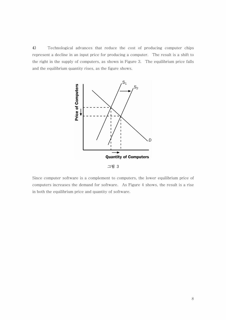
4) Technological advances that reduce the cost of producing computer chips

represent a decline in an input price for producing a computer. The result is a shift to

the right in the supply of computers, as shown in Figure 3. The equilibrium price falls

and the equilibrium quantity rises, as the figure shows.

그림 3

Since computer software is a complement to computers, the lower equilibrium price of

computers increases the demand for software. As Figure 4 shows, the result is a rise

in both the equilibrium price and quantity of software.

9

그림 4

Since typewriters are substitutes for computers, the lower equilibrium price of

computers reduces the demand for typewriters. As Figure 5 shows, the result is a

decline in both the equilibrium price and quantity of typewriters.

그림 5

10

8)

a. Cigars and chewing tobacco are substitutes for cigarettes, since a higher price

for cigarettes would increase the demand for cigars and chewing tobacco.

b. An increase in the tax on cigarettes leads to increased demand for cigars and

chewing tobacco. The result, as shown in Figure 25 for cigars, is a rise in both the

equilibrium price and quantity of cigars and chewing tobacco.

c. The results in part (b) showed that a tax on cigarettes leads people to

substitute cigars and chewing tobacco for cigarettes when the tax on cigarettes rises.

To reduce total tobacco usage, policymakers might also want to increase the tax on

cigars and chewing tobacco, or pursue some type of public education program.

11)

a. As Figure 6 shows, the supply curve is vertical. The constant quantity

supplied makes sense because the basketball arena has a fixed number of seats no

matter what the price.

그림 6

11

Figure 31

b. Quantity supplied equals quantity demanded at a price of $8. The equilibrium

quantity is 8,000 tickets.

c.

Price Quantity Demanded Quantity Supplied

$ 4 14,000 8,000

8 11,000 8,000

12 8,000 8,000

16 5,000 8,000

20 2,000 8,000

The new equilibrium price will be $12, which equates quantity demanded to quantity

supplied. The equilibrium quantity is 8,000 tickets.

13) Equilibrium occurs where quantity demanded is equal to quantity supplied.

Thus:

Qd = Qs

1,600 – 300P = 1,400 + 700P

200 = 1,000P

P = $0.20

Qd = 1,600 – 300(0.20) = 1,600 – 60 = 1,540

Qs = 1,400 + 700(0.20) = 1,400 + 140 = 1,540.

The equilibrium price of a chocolate bar is $0.20 and the equilibrium quantity is 1,5

40 bars.

12

Chapter 5:

2)

a. For business travelers, the price elasticity of demand when the price of tickets

rises from $200 to $250 is [(2,000 - 1,900)/1,950]/[(250 - 200)/225] = 0.05/0.22 =

0.23. For vacationers, the price elasticity of demand when the price of tickets rises

from $200 to $250 is [(800 - 600)/700] / [(250 - 200)/225] = 0.29/0.22 = 1.32.

b. The price elasticity of demand for vacationers is higher than the elasticity for

business travelers because vacationers can choose more easily a different mode of

transportation (like driving or taking the train). Business travelers are less likely to do

so since time is more important to them and their schedules are less adaptable.

3)

a. If your income is $10,000, your price elasticity of demand as the price of

compact discs rises from $8 to $10 is [(40 - 32)/36]/[(10 - 8)/9] =0.22/0.22 = 1. If

your income is $12,000, the elasticity is [(50 - 45)/47.5]/[(10 - 8)/9] = 0.11/0.22 = 0.5.

b. If the price is $12, your income elasticity of demand as your income increases

from $10,000 to $12,000 is [(30 - 24)/27] / [(12,000 - 10,000)/11,000] = 0.22/0.18 =

1.22. If the price is $16, your income elasticity of demand as your income increases

from $10,000 to $12,000 is [(12 - 8)/10] / [(12,000 - 10,000)/11,000] = 0.40/0.18 =

2.2.

5)

a. With a 4.3 percent decline in quantity following a 20 percent increase in price,

the price elasticity of demand is only 4.3/20 = 0.215, which is fairly inelastic.

b. With inelastic demand, the Transit Authority's revenue rises when the fare

rises.

c. The elasticity estimate might be unreliable because it is only the first month

after the fare increase. As time goes by, people may switch to other means of

transportation in response to the price increase. So the elasticity may be larger in the

long run than it is in the short run.

13

6) Tom's price elasticity of demand is zero, since he wants the same quantity

regardless of the price. Jerry's price elasticity of demand is one, since he spends the

same amount on gas, no matter what the price, which means his percentage change in

quantity is equal to the percentage change in price.

7) To explain the fact that spending on restaurant meals declines more during

economic downturns than does spending on food to be eaten at home, economists look

at the income elasticity of demand. In economic downturns, people have lower income.

To explain the fact, the income elasticity of restaurant meals must be larger than the

income elasticity of spending on food to be eaten at home.

8)

a. With a price elasticity of demand of 0.4, reducing the quantity demanded of

cigarettes by 20 percent requires a 50 percent increase in price, since 20/50 = 0.4.

With the price of cigarettes currently $2, this would require an increase in the price to

$3.33 a pack using the midpoint method (note that ($3.33 - $2)/$2.67 = .50).

b. The policy will have a larger effect five years from now than it does one year

from now. The elasticity is larger in the long run, since it may take some time for

people to reduce their cigarette usage. The habit of smoking is hard to break in the

short run.

c. Since teenagers don't have as much income as adults, they are likely to have a

higher price elasticity of demand. Also, adults are more likely to be addicted to

cigarettes, making it more difficult to reduce their quantity demanded in response to a

higher price.

Chapter 6

4)

a. Figure 4 shows the market for beer without the tax. The equilibrium price is

P1 and the equilibrium quantity is Q1. The price paid by consumers is the same as the

price received by producers.

14

Figure 4

Figure 5

b. When the tax is imposed, it drives a wedge of $2 between supply and demand,

as shown in Figure 5. The price paid by consumers is P2, while the price received by

producers is P2 – $2. The quantity of beer sold declines to Q2.

15

5) Reducing the payroll tax paid by firms and using part of the extra revenue to

reduce the payroll tax paid by workers would not make workers better off, because the

division of the burden of a tax depends on the elasticity of supply and demand and not

on who must pay the tax. Since the tax wedge would be larger, it is likely that both

firms and workers, who share the burden of any tax, would be worse off.

6) If the government imposes a $500 tax on luxury cars, the price paid by

consumers will rise less than $500, in general. The burden of any tax is shared by

both producers and consumers⎯the price paid by consumers rises and the price

received by producers falls, with the difference between the two equal to the amount of

the tax. The only exceptions would be if the supply curve were perfectly elastic or the

demand curve were perfectly inelastic, in which case consumers would bear the full

burden of the tax and the price paid by consumers would rise by exactly $500.

7)

a. It doesn’t matter whether the tax is imposed on producers or consumers⎯the

effect will be the same. With no tax, as shown in Figure 6, the demand curve is D1 and

the supply curve is S1. If the tax is imposed on producers, the supply curve shifts up

by the amount of the tax (50 cents) to S2. Then the equilibrium quantity is Q2, the

price paid by consumers is P2, and the price received (after taxes are paid) by

producers is P2 – 50 cents. If the tax is instead imposed on consumers, the demand

curve shifts down by the amount of the tax (50 cents) to D2. The downward shift in

the demand curve (when the tax is imposed on consumers) is exactly the same

magnitude as the upward shift in the supply curve when the tax is imposed on

producers. So again, the equilibrium quantity is Q2, the price paid by consumers is P2

(including the tax paid to the government), and the price received by producers is P2 –

50 cents.

16

Figure 6

b. The more elastic is the demand curve, the more effective this tax will be in

reducing the quantity of gasoline consumed. Greater elasticity of demand means that

quantity falls more in response to the rise in the price of gasoline. Figure 7 illustrates

this result. Demand curve D1 represents an elastic demand curve, while demand curve

D2 is more inelastic. To get the same tax wedge between demand and supply requires

a greater reduction in quantity with demand curve D1 than for demand curve D2.

Figure 7

17

c. The consumers of gasoline are hurt by the tax because they get less gasoline

at a higher price.

d. Workers in the oil industry are hurt by the tax as well. With a lower quantity

of gasoline being produced, some workers may lose their jobs. With a lower price

received by producers, wages of workers might decline.

8)

a. Figure 8 shows the effects of the minimum wage. In the absence of the

minimum wage, the market wage would be w1 and Q1 workers would be employed.

With the minimum wage (wm) imposed above w1, the market wage is wm, the number of

employed workers is Q2, and the number of workers who are unemployed is Q3 - Q2.

Total wage payments to workers are shown as the area of rectangle ABCD, which

equals wm times Q2.

Figure 8

b. An increase in the minimum wage would decrease employment. The size of

the effect on employment depends only on the elasticity of demand. The elasticity of

supply doesn’t matter, because there’s a surplus of labor.

18

c. The increase in the minimum wage would increase unemployment. The size of

the rise in unemployment depends on both the elasticities of supply and demand. The

elasticity of demand determines the quantity of labor demanded, the elasticity of supply

determines the quantity of labor supplied, and the difference between the quantity

supplied and demanded of labor is the amount of unemployment.

d. If the demand for unskilled labor were inelastic, the rise in the minimum wage

would increase total wage payments to unskilled labor. With inelastic demand, the

percentage decline in employment would be less than the percentage increase in the

wage, so total wage payments increase. However, if the demand for unskilled labor

were elastic, total wage payments would decline, since then the percentage decline in

employment would exceed the percentage increase in the wage.

11)

a. The effect of a $0.50 per cone subsidy is to shift the demand curve up by $0.50

at each quantity, since at each quantity a consumer's willingness to pay is $0.50 higher.

The effects of such a subsidy are shown in Figure 14. Before the subsidy, the price is

P1. After the subsidy, the price received by sellers is PS and the effective price paid

by consumers is PD, which equals PS minus 50 cents. Before the subsidy, the quantity

of cones sold is Q1; after the subsidy the quantity increases to Q2.

Figure 14

19

b. Because of the subsidy, consumers are better off, since they consume more at

a lower price. Producers are also better off, since they sell more at a higher price.

The government loses, since it has to pay for the subsidy.

Chapter 7:

1) If an early freeze in California sours the lemon crop, the supply curve for

lemons shifts to the left, as shown in Figure 5. The result is a rise in the price of

lemons and a decline in consumer surplus from A + B + C to just A. So consumer

surplus declines by the amount B + C.

Figure 5

In the market for lemonade, the higher cost of lemons reduces the supply of lemonade,

as shown in Figure 6. The result is a rise in the price of lemonade and a decline in

consumer surplus from D + E + F to just D, a loss of E + F. Note that an event that

affects consumer surplus in one market often has effects on consumer surplus in other

markets.

20

Figure 6

2) A rise in the demand for French bread leads to an increase in producer surplus

in the market for French bread, as shown in Figure 7. The shift of the demand curve

leads to an increased price, which increases producer surplus from area A to area A +

B + C.

Figure 7

21

The increased quantity of French bread being sold increases the demand for flour, as

shown in Figure 8. As a result, the price of flour rises, increasing producer surplus

from area D to D + E + F. Note that an event that affects producer surplus in one

market leads to effects on producer surplus in related markets.

Figure 8

4) a. Ernie’s supply schedule for water is:

Price Quantity Supplied

More than $7 4

$5 to $7 3

$3 to $5 2

$1 to $3 1

Less than $1 0

22

Ernie’s supply curve is shown in Figure 10.

Figure 10

b. When the price of a bottle of water is $4, Ernie sells two bottles of water. His

producer surplus is shown as area A in the figure. He receives $4 for his first bottle of

water, but it costs only $1 to produce, so Ernie has producer surplus of $3. He also

receives $4 for his second bottle of water, which costs $3 to produce, so he has

producer surplus of $1. Thus Ernie’s total producer surplus is $3 + $1 = $4, which is

the area of A in the figure.

c. When the price of a bottle of water rises from $4 to $6, Ernie sells three bottles

of water, an increase of one. His producer surplus consists of both areas A and B in

the figure, an increase by the amount of area B. He gets producer surplus of $5 from

the first bottle ($6 price minus $1 cost), $3 from the second bottle ($6 price minus $3

cost), and $1 from the third bottle ($6 price minus $5 price), for a total producer surplus

of $9. Thus producer surplus rises by $5 (which is the size of area B) when the price

of a bottle of water rises from $4 to $6.

6) a. The effect of falling production costs in the market for stereos results

in a shift to the right in the supply curve, as shown in Figure 11. As a result, the

equilibrium price of stereos declines and the equilibrium quantity increases.

23

b. The decline in the price of stereos increases consumer surplus from area A to

A + B + C + D, an increase in the amount B + C + D. Prior to the shift in supply,

producer surplus was areas B + E (the area above the supply curve and below the

price). After the shift in supply, producer surplus is areas E + F + G. So producer

surplus changes by the amount F + G – B, which may be positive or negative. The

increase in quantity increases producer surplus, while the decline in the price reduces

producer surplus. Since consumer surplus rises by B + C + D and producer surplus

rises by F + G – B, total surplus rises by C + D + F + G.

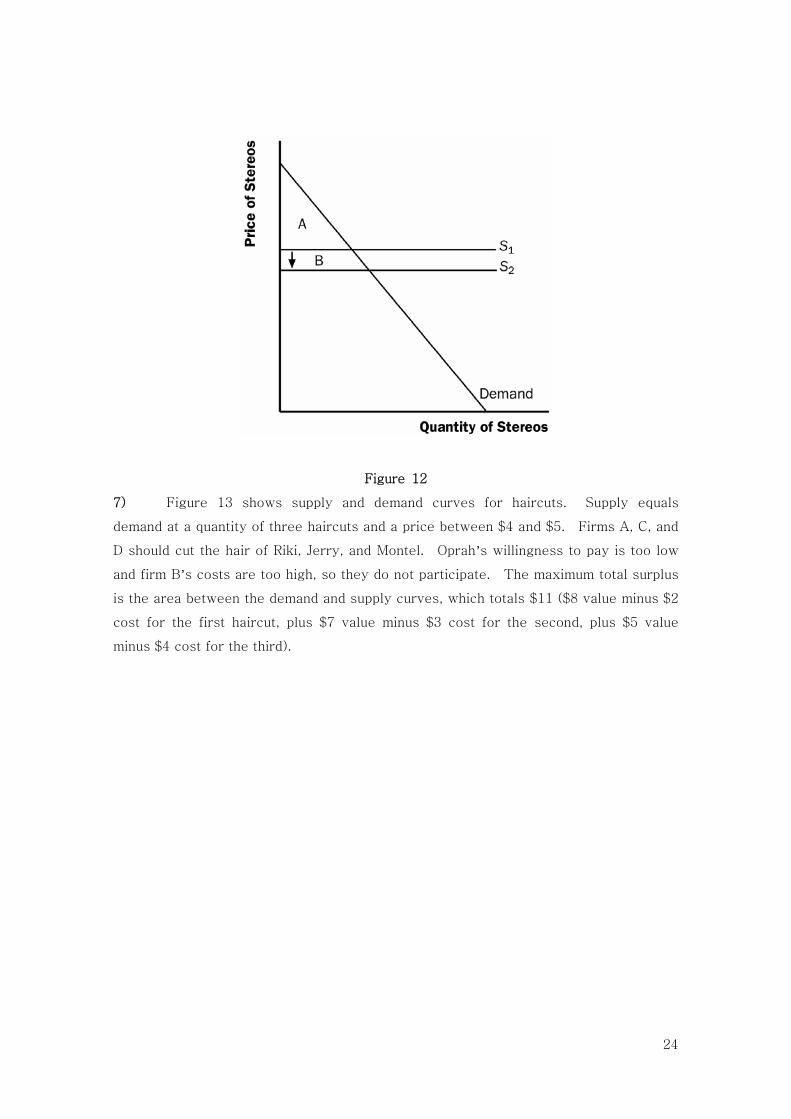
c. If the supply of stereos is very elastic, then the shift of the supply curve

benefits consumers most. To take the most dramatic case, suppose the supply curve

were horizontal, as shown in Figure 12. Then there is no producer surplus at all.

Consumers capture all the benefits of falling production costs, with consumer surplus

rising from area A to area A + B.

Figure 11

24

Figure 12

7) Figure 13 shows supply and demand curves for haircuts. Supply equals

demand at a quantity of three haircuts and a price between $4 and $5. Firms A, C, and

D should cut the hair of Riki, Jerry, and Montel. Oprah’s willingness to pay is too low

and firm B’s costs are too high, so they do not participate. The maximum total surplus

is the area between the demand and supply curves, which totals $11 ($8 value minus $2

cost for the first haircut, plus $7 value minus $3 cost for the second, plus $5 value

minus $4 cost for the third).

25

Figure 13

8)

a. The effect of falling production costs in the market for computers results in a

shift to the right in the supply curve, as shown in Figure 14. As a result, the

equilibrium price of computers declines and the equilibrium quantity increases. The

decline in the price of computers increases consumer surplus from area A to A + B + C

+ D, an increase in the amount B + C + D.

26

Figure 14

Prior to the shift in supply, producer surplus was areas B + E (the area above the

supply curve and below the price). After the shift in supply, producer surplus is areas

E + F + G. So producer surplus changes by the amount F + G – B, which may be

positive or negative. The increase in quantity increases producer surplus, while the

decline in the price reduces producer surplus. Since consumer surplus rises by B + C

+ D and producer surplus rises by F + G – B, total surplus rises by C + D + F + G.

Figure 15

27

b. Since adding machines are substitutes for computers, the decline in the price of

computers means that people substitute computers for adding machines, shifting the

demand for adding machines to the left, as shown in Figure 15. The result is a decline

in both the equilibrium price and equilibrium quantity of adding machines. Consumer

surplus in the adding-machine market changes from area A + B to A + C, a net change

of C – B. Producer surplus changes from area C + D + E to area E, a net loss of C +

D. Adding machine producers are sad about technological advance in computers

because their producer surplus declines.

c. Since software and computers are complements, the decline in the price and

increase in the quantity of computers means that the demand for software increases,

shifting the demand for software to the right, as shown in Figure 16. The result is an

increase in both the price and quantity of software. Consumer surplus in the software

market changes from B + C to A + B, a net change of A – C. Producer surplus

changes from E to C + D + E, an increase of C + D, so software producers should be

happy about the technological progress in computers.

d. Yes, this analysis helps explain why Bill Gates is one the world’s richest men,

since his company produces a lot of software that is a complement with computers and

there has been tremendous technological advance in computers.

Figure 16

28

Chapter 9

2)

a. The statement, "If the government taxes land, wealthy landowners will pass the

tax on to their poorer renters," is incorrect. With a tax on land, landowners can not

pass the tax on. Since the supply curve of land is perfectly inelastic, landowners bear

the entire burden of the tax. Renters will not be affected at all.

b. The statement, "If the government taxes apartment buildings, wealthy

landowners will pass the tax on to their poorer renters," is partially correct. With a tax

on apartment buildings, landowners can pass the tax on more easily, though the extent

to which they do this depends on the elasticities of supply and demand. In this case,

the tax is a direct addition to the cost of rental units, so the supply curve will shift up

by the amount of the tax. The tax will be shared by renters and landowners,

depending on the elasticities of demand and supply.

3)

a. The statement, "A tax that has no deadweight loss cannot raise any revenue for

the government," is incorrect. An example is the case of a tax when either supply or

demand is perfectly inelastic. The tax has neither an effect on quantity nor any

deadweight loss, but it does raise revenue.

b. The statement, "A tax that raises no revenue for the government cannot have

any deadweight loss," is incorrect. An example is the case of a 100 percent tax

imposed on sellers. With a 100 percent tax on their sales of the good, sellers won't

supply any of the good, so the tax will raise no revenue. Yet the tax has a large

deadweight loss, since it reduces the quantity sold to zero.

5)

a. The deadweight loss from a tax on heating oil is likely to be greater in the fifth

year after it is imposed rather than the first year. In the first year, the elasticity of

demand is fairly low, as people who own oil heaters are not likely to get rid of them

right away. But over time they may switch to other energy sources and people buying

new heaters for their homes will more likely choose gas or electric, so the tax will have

a greater impact on quantity.

29

b. The tax revenue is likely to be higher in the first year after it is imposed than

in the fifth year. In the first year, demand is more inelastic, so the quantity does not

decline as much and tax revenue is relatively high. As time passes and more people

substitute away from oil, the equilibrium quantity declines, as does tax revenue.

8)

a. Figure 6 illustrates the market for socks and the effects of the tax. Without a

tax, the equilibrium quantity would be Q1, the equilibrium price would be P1, total

spending by consumers equals total revenue for producers, which is P1 x Q1, which

equals area B+C+D+E+F, and government revenue is zero. The imposition of a tax

places a wedge between the price buyers pay, PB, and the price sellers receive, PS,

where PB = PS + tax. The quantity sold declines to Q2. Now total spending by

consumers is PB x Q2, which equals area A+B+C+D, total revenue for producers is PS

x Q2, which is area C+D, and government tax revenue is Q2 x tax, which is area A+B.

b. Unless supply is perfectly elastic, the price received by producers falls

because of the tax. Total receipts for producers fall, since producers lose revenue

equal to area B+E+F.

Figure 6

30

c. The price paid by consumers rises, unless demand is perfectly elastic.

Whether total spending by consumers rises or falls depends on the price elasticity of

demand. If demand is elastic, the percentage decline in quantity exceeds the

percentage increase in price, so total spending declines. If demand is inelastic, the

percentage decline in quantity is less than the percentage increase in price, so total

spending rises. Whether total consumer spending falls or rises, consumer surplus

declines because of the increase in price and reduction in quantity.

11)

a. Setting quantity supplied equal to quantity demanded gives 2P = 300 – P.

Adding P to both sides of the equation gives 3P = 300. Dividing both sides by 3 gives

P = 100. Plugging P = 100 back into either equation for quantity demanded or supplied

gives Q = 200.

b. Now P is the price received by sellers and P+T is the price paid by buyers.

Equating quantity demanded to quantity supplied gives 2P = 300 - (P+T). Adding P to

both sides of the equation gives 3P = 300 – T. Dividing both sides by 3 gives P = 100

- T/3. This is the price received by sellers. The buyers pay a price equal to the

price received by sellers plus the tax (P+T = 100 + 2T/3). The quantity sold is now Q

= 2P = 200 – 2T/3.

c. Since tax revenue is equal to T x Q and Q = 200 - 2T/3, tax revenue equals

200T - 2T2/3. Figure 9 shows a graph of this relationship. Tax revenue is zero at T

= 0 and at T = 300.

Figure 9

31

d. As Figure 10 shows, the area of the triangle (laid on its side) that represents

the deadweight loss is 1/2 x base x height, where the base is the change in the price,

which is the size of the tax (T) and the height is the amount of the decline in quantity

(2T/3). So the deadweight loss equals 1/2 x T x 2T/3 = T2/3. This rises

exponentially from 0 (when T = 0) to 45,000 when T = 300, as shown in Figure 11.

Figure 10

Figure 11

32

e. A tax of $200 per unit is a bad idea, because it's in a region in which tax

revenue is declining. The government could reduce the tax to $150 per unit, get more

tax revenue ($15,000 when the tax is $150 versus $13,333 when the tax is $200), and

reduce the deadweight loss (7,500 when the tax is $150 compared to 13,333 when the

tax is $200).

Chapter 9

3) Figure 5 shows the market for cotton in countries A and B. Note that the

world price of cotton is the same in both countries. Country A imports cotton from

country B. The table below shows that total surplus is higher in both countries.

However, in country A, consumers are better off and producers are worse off, while in

country B, consumers are worse off and producers are better off.

Figure 5

COUNTRY A

Before Trade After Trade CHANGE

Consumer Surplus C C+D+F +(D+F)

Producer Surplus D+E E –D

Total Surplus C+D+E C+D+E+F +F

33

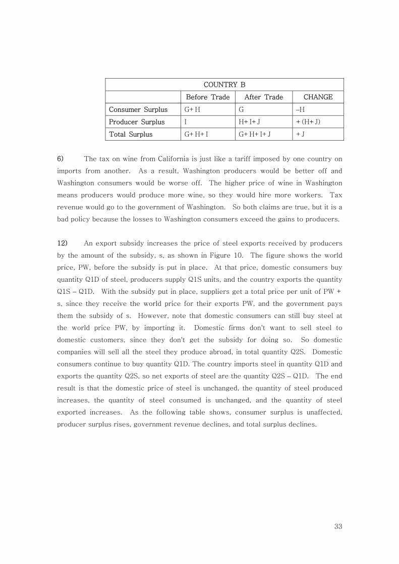
COUNTRY B

Before Trade After Trade CHANGE

Consumer Surplus G+H G –H

Producer Surplus I H+I+J +(H+J)

Total Surplus G+H+I G+H+I+J +J

6) The tax on wine from California is just like a tariff imposed by one country on

imports from another. As a result, Washington producers would be better off and

Washington consumers would be worse off. The higher price of wine in Washington

means producers would produce more wine, so they would hire more workers. Tax

revenue would go to the government of Washington. So both claims are true, but it is a

bad policy because the losses to Washington consumers exceed the gains to producers.

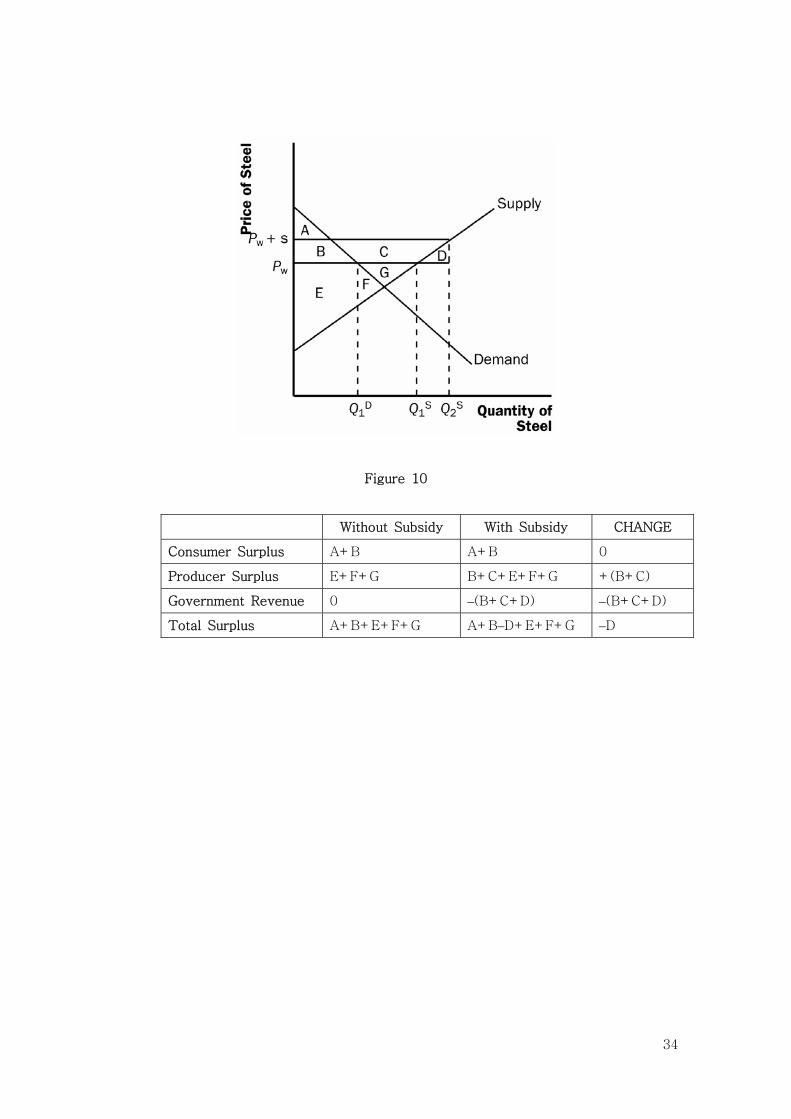
12) An export subsidy increases the price of steel exports received by producers

by the amount of the subsidy, s, as shown in Figure 10. The figure shows the world

price, PW, before the subsidy is put in place. At that price, domestic consumers buy

quantity Q1D of steel, producers supply Q1S units, and the country exports the quantity

Q1S – Q1D. With the subsidy put in place, suppliers get a total price per unit of PW +

s, since they receive the world price for their exports PW, and the government pays

them the subsidy of s. However, note that domestic consumers can still buy steel at

the world price PW, by importing it. Domestic firms don't want to sell steel to

domestic customers, since they don't get the subsidy for doing so. So domestic

companies will sell all the steel they produce abroad, in total quantity Q2S. Domestic

consumers continue to buy quantity Q1D. The country imports steel in quantity Q1D and

exports the quantity Q2S, so net exports of steel are the quantity Q2S – Q1D. The end

result is that the domestic price of steel is unchanged, the quantity of steel produced

increases, the quantity of steel consumed is unchanged, and the quantity of steel

exported increases. As the following table shows, consumer surplus is unaffected,

producer surplus rises, government revenue declines, and total surplus declines.

34

Figure 10

Without Subsidy With Subsidy CHANGE

Consumer Surplus A+B A+B 0

Producer Surplus E+F+G B+C+E+F+G +(B+C)

Government Revenue 0 –(B+C+D) –(B+C+D)

Total Surplus A+B+E+F+G A+B–D+E+F+G –D