Another Look at the Consumer Price Index - A wavelet Approach

Mathematical Theory and Modeling www.iiste.org

ISSN 2224-5804 (Paper) ISSN 2225-0522 (Online)

Vol.6, No.10, 2016

32

Another Look at the Consumer Price Index - A wavelet Approach

1I.A.Iwok and

2G.M.Udoh

1Department of Mathematics/Statistics, University of Port-Harcourt, P.M.B.5323, Port-

Harcourt, Rivers State; Nigeria.

2Department of Statistics, Akwa Ibom State Polytechnic, Ikot Osurua

Abstract

A wavelet approach was applied to a consumer price index (CPI) series to address the

draw backs of some periodic models. The method requires no assumption of the data

generating process but involves the spliting of a given signal into several components with

each component reflecting the evolution trough of the signal at a particular time. The multi-

level stationary Haar wavelet decomposition was applied to the series which gave rise to a

dyadic sequence of 28 , and the series was decomposed accordingly using a computer

program written for the purpose. Multi-resolution wavelet method was then used to

reconstruct the series and the significant details (𝑑𝑗,𝑡) that captured the season were added to

the trend (𝑠𝑗,𝑡) component for the estimatation of the series {𝑌𝑡}. The resulting wavelet

model was subjected to diagnostic checks and were found to be adequate. Comparative study

was carried out with some hilighted CPI models built by some researchers. It was discovered

that the wavelet models performs better.

Keywords: Mother wavelets, Haar wavelet decomposition, Multi-resolution, Auto-

correlation and Partial auto-correlation function.

brought to you by COREView metadata, citation and similar papers at core.ac.uk

provided by International Institute for Science, Technology and Education (IISTE): E-Journals

https://core.ac.uk/display/234680483?utm_source=pdf&utm_medium=banner&utm_campaign=pdf-decoration-v1

http://www.iiste.org/



Vol.6, No.10, 2016

33

1.0 Introduction/Review

Consumer price index (CPI) is an economic indicator that gives a comprehensive

measure used for the estimation of price changes in a basket of goods and services

representative of consumption expenditure in an economy. It measures changes in the price

level of a market basket of consumer goods and services purchased by households.

Statistically, it is an estimate constructed using the prices of a sample of representative items

whose prices are collected periodically. The percentage change in the CPI over a period of

time gives the amount of inflation over that specific period. Thus, the CPI provides a measure

of inflation.

In recent years, inflation has become one of the major economic focus of most

countries of the world, especially those in Africa and Asia. Due to its impact on the nation’s

economy, the control of inflation has become imperative for any nation. To control inflation

in the future, there is need to relate the past and the present effect. A body of techniques that

can be used for such predictive purposes is time series.

According to Abraham (2014), Consumer price index (CPI) measures changes in the

price level of market basket of consumer goods and services purchased by households over a

period of time. Abraham (2014) modelled the CPI using Fourier series approach. The

approach identified the period to be 12 with a frequency of 0.02678. The Fourier series model

was subjected to some diagnostic checks and was found to be adequate. However, the root

mean square error was found to be moderately high with a value of 7.2587.

In particular, Akpanta and Okorie (2015) modeled the Nigerian CPI in the time-

domain using the Seasonal Autoregressive Integrated Moving Average model (SARIMA). In

this case, the seasonal component of the series was assumed to be stochastic and correlated




Vol.6, No.10, 2016

34

with non-seasonal components. Despite the correlation structure, the model was still found to

be adequate with a root means square error of 4.2345.

Taking into consideration the periodic variation found in the data, Omekara et al

(2013), Nachane and clavel (2014) modeled inflation rate in the frequency domain using the

Mixed Fourier series and the ARMA Model with Fourier coefficients respectively. The work

showed that the residuals followed a white noise process, indicating a good fit of the model.

In Nigeria, the CPI is calculated by the National Bureau of Statistics and assisted by

the Central Bank of Nigeria. It is one of the most frequently used statistics for identifying

periods of inflation and deflation and can be used to index the real values of wages and

salaries. However, since most financial data like the CPI are usually defective in terms of

irregular characteristics, the data is usually smoothened by log transformation, differencing or

filtering before analysis is carried out. According to Al Wadi et al (2010), one of such

filtering approaches in the frequency domain is wavelet analysis.

A Wavelet is a function which enables us to split the given signal into several

frequency components, each reflecting the evolution trough time of the signal at a particular

frequency. Wavelet as its name suggests, is a small wave. In this context, the term "small"

essentially means that the wave grows and decays in a limited time frame.

Masset (2008) considered wavelet as a very potent method in studying financial data

or variable that exhibit a cyclical behaviour and/or affected by a seasonal effects. He applied

the wavelet method in the analysis of several seasonal data and it was discovered that wavelet

methods produced reliable results than the linear models.

The spread in the acceptability of Wavelet analysis is seen in its adoption by Wall

Street analysts as a veritable mathematical tools for analyszing financial data (Manahanda et




Vol.6, No.10, 2016

35

al, 2007). The range of the application of wavelet in the financial data is potentially used in

denoising and seasonal filtering, identification of regimes shift and jumps.

According to Mallet (2001), Gencay et al (2002) and Crowdly (2005), Wavelet

analysis takes its root from Filter and Fourier analysis and is able to overcome most of the

limitations of Fourier series analysis. This is because, they can combine information from

both time-domain and frequency-domain, and do not require assumptions concerning the data

generating process.

Because of the drawbacks of Fourier or Spectral Analysis, Masset (2008) presented a

set of tools which allows gathering information about the frequency components. This method

was able to address the problem of the drawbacks of spectral analysis temporarily.

Yogo (2003) in his paper, pointed out that Multiresolution wavelet analysis is a

natural way of decomposing economic time series into components of various frequencies

which are long-run trend, business-cycle component and high frequency noise. The paper was

applied to the real Gross National Product and inflation and was found to address the

limitations of the Fourier models.

Renaud et al (2004) took a critical look at the Wavelet-Based method for time series.

The work was based on multiple decomposition of signal using a redundant (a trous) wavelets

transform which has the advantage of being shift-invariant. The result was a decomposition of

the signal into range of frequency scales which explicitly showed that the method works well

and adapts itself to studies involving financial data. It was also discovered that in a series

whose dynamics is made of Autoregressive integrated moving average (ARIMA) model and 𝑠

cyclical components, the wavelet analysis can be used to remove the impact of trend, noise

and the seasonality.




Vol.6, No.10, 2016

36

In the same vein, Mehala and Dahiya (2013) revealed that the Wavelet transform are

capable of revealing detailed aspects of data such as trends, breakdown points, discontinuities

in higher derivatives and self-similarity which cannot be adduced using Fourier transform.

Perhaps it was such findings which encouraged Mukhopadhyay et al (2013) to adopt

Wavelet transform in the study of wind speed data. The study used continuous Wavelet

transform (MCWT) like Morlet to check the periodicity of wind speed. It was shown that

wavelet transform provided more information about signal constituents of the dynamic

speckle.

As spelt out in the review; except the wavelet approach, several time series techniques

have been applied in modelling the CPI series. Non of this techniques actually reflected the

evolution trough time of the signal at a particular frequency. This work therefore seeks to

address the CPI series in another dimension using the wavelet platform.

2.0 Methodology

2.1 Wavelets

A Wavelet is a function which enables us to split a given signal into several

components, each reflecting the evolution trough time of the signal at a particular time.The

essence of wavelet analysis consists of projecting the time series of interest [𝑌𝑡] =

0,1,2, … , (N − 1) onto a discrete wavelet filter often called the mother wavelet. The mother

wavelet is represented as:

[ℎ𝑙] = (ℎ0, ℎ1, … , ℎ𝐿−1, 0, … ,0)

The discrete wavelet filter satisfies the properties:

1. ∑ ℎ𝑙 = 0𝐿−1𝑙=0 (1)




Vol.6, No.10, 2016

37

2. ∑ ℎ𝑙2 = 0𝐿−1

𝑙=0 (2)

3. ∑ ℎ𝑙ℎ𝑙+2n = 0 ∀ non − zero integers𝐿−1𝑙=0 𝑛 (3)

where L is a suitably chosen positive integer and 𝐿 < 𝑁 and padded with zeros at the end so

that it has the same dimension N as [𝑌𝑡].

By virtue of (1), [ℎ𝑙] is a high-pass filter. Associated with [ℎ𝑙] is a scaling filter (or father

wavelet) which is a low-pass filter, recoverable from [ℎ𝑙] via the relationship

𝑔𝑙 = (−1)𝑙+1ℎ𝐿−1−𝑙 ; 𝑙 = 0,1, … , 𝐿 − 1 (4)

Following Daubechies (1992), Db1 wavelet fliter which is equivalent to Haar wavelets filter

can be represented as:

𝜓(𝑦) = 1, if 𝑦 𝜖 [0 , 0.5]

𝜓(𝑦) = −1, if 𝑦 𝜖 [0.5 , 1]

𝜓(𝑦) = 1, if 𝑦 ∉ [0 , 0.5]

ψ(𝑦) = 1, if 𝑦 𝜖 [0 , 1]

𝜓(𝑦) = 0, if 𝑦 ∉ [0 , 1]

The Haar wavelet is the first and the simplest. Haar wavelet is discontinuous and

resembles a step function. For prediction purposes, we use the stationary discrete wavelet

transform introduced by Masset (2008). The coefficients can be obtained via a pyramid

algorithm and the wavelet coefficients at each level 𝑗 comprise 𝑁 elements.

The algorithm yields the 𝑁 − dimensional vector of wavelet coefficients

𝑤𝑡 = (𝑤𝑡(1)

, 𝑤𝑡(2)

, … , 𝑤𝑡(𝑗)

, 𝑣𝑡𝑗)𝑇

(5) ;




Vol.6, No.10, 2016

38

where the 𝑁 2𝑗⁄ vector {𝑤𝑡(𝑗)

} can be interpreted as the vector of wavelet coefficients

associated with the dynamics of the series {𝑌𝑡} on a scale of length 𝜆𝑗 = 2𝑗−1, (with

increasing scales corresponding to lower frequencies) and {𝑣𝑡(𝑗)

} represents the averages on

the scale of length 2𝑗.

2.2 White Noise Process

A process {𝜀𝑡} is said to be a white noise process with mean 0 and variance 𝜎𝜀2 written

{𝜀𝑡}~𝑊𝑁(0, 𝜎𝜀2 ), if it is a sequence of uncorrelated random variables from a fixed

distribution.

2.3 Multi-resolution

Multi-resolution represents a convenient way of decomposing a given series {𝑌𝑡} into

changes attributable at different scales.

Let the filter coefficients be expressed in reverse order as:

𝑞1 = (ℎ𝑁 , ℎ𝑁−1, … , ℎ1, ℎ0)T

Let 𝑞𝑗 denote the zero-padded scale 𝑗 wavelet filter coefficients obtained by 𝑗

convolutions of 𝑞1 with itself and let 𝜑𝑗 represent the N2j⁄ × N matrix of “circularly

shifted” coefficients of 𝑞1 (by a factor of 2𝑗).

We can now write the 𝑁 × 𝑁 matrix 𝜑 as

[ 𝜑1

𝜑2⋯⋮⋯𝜑𝑗

𝜗𝑗 ]

= 𝜑




Vol.6, No.10, 2016

39

where,

𝜗𝑗 is 𝑁 × 𝑁 vector with each term equal to 1 √𝑁⁄ .

The multi-resolution scale defines the 𝑗 th level wavelet detail 𝑑𝑗,𝑡 as:

𝑑𝑗,𝑡 = 𝜑𝑗𝑇𝑤𝑡

(𝑗), 𝑗 = 1,2, … , 𝐽 (6)

where 𝑤𝑡(𝑗)

are the wavelet coefficients at the 𝑗th scale defined in (5).

The wavelet smooth is defined as:

𝑠𝑗,𝑡 = 𝜗𝑗𝑇𝑣𝑡

(𝑗) (7)

Hence, the multi-resolution Wavelet can now be expressed by the relationship:

Y𝑡 = ∑ 𝑑𝑗,𝑡Jj=1 + 𝑠𝑗,𝑡 + εt (8)

where εt is a white noise process.

That is, each observation in the series is additively decomposed into the 𝐽 wavelet details and

the wavelet smooth.

2.4 Diagnostic Check of the Model

The diagnostic check is based on the behaviour of the residuals obtained from fitting

the model. For model adequacy, the residuals are expected to be uncorrelated at the various

lags. These non correlated random varables can be confirmed if the Autocorrelation Function

(ACF) plot and Partial Autocorrelation Function ( PACF) plot does not show any spike above

or below the 95% confidence interval.




Vol.6, No.10, 2016

40

3.0 Data Analysis

The data was obtained from the Central bank of Nigerian official web site

(www.cbn.gov.ng). The analysis was done using Minitab and Matlab softwares.

3.1 The Wavelet Model

The raw data plot (figure 1) shows clearly that the series {𝑌𝑡} is non-stationary and

contains trend. The behaviour of the Autocorrelation and Partial Autocorrelation functions

(figures 2 and 3) suggest an 𝐴𝑅𝐼𝑀𝐴(1, 0, 0) model for {𝑌𝑡}. Also, the Autocorrelation

function (figure 2) exhibit significant spikes at lag 12, 24, 36,… . This shows that the series is

seasonal and since the series is a monthly data; the season 𝑠 = 12. Hence, the series {𝑌𝑡}

contains trend, noise and seasonality. According to Renaud et al (2004), for a series {𝑌𝑡}

whose dynamics is made of 𝐴𝑅𝐼𝑀𝐴(1, 0, 0) and 𝑠 = 12 cyclical components, the wavelet

analysis can be used to remove these irregularities.

The Matlab script in Appendix A was used to decompose the series {𝑌𝑡} into trend,

seasonal and the error component. The series {𝑌𝑡} contains 256 data points which give rise to

a dyadic sequence {2𝐽 ; i. e. 28}. This means that we can decompose the data set until level

8. Nevertheless, it was found that level 3 and upward had similar results. Therefore the series

was decomposed until level 3 as suggested by Daubechies (1992). The multi-level stationary

Haar wavelet decomposition was applied to the data set. The multiresolution wavelet analysis

was then used to reconstruct the series and the significant details (𝑑𝑗,𝑡) that captured the

seasonal period ( see figure 4 and 5 ) were added to the smooth or trend (𝑠𝑗,𝑡) so as to estimate

{𝑌𝑡}.

At scale 𝑗, the wavelet detail 𝑑𝑗 captures frequencies 12𝑗+1⁄ ≤ 𝑓 ≤ 1

2𝑗⁄ and the

wavelet smooth 𝑠𝑗 captures frequencies 𝑓 < 12𝑗⁄ . The level three multi-resolution captures


http://www.cbn.gov.ng/



Vol.6, No.10, 2016

41

the components of the time series which have a frequency 𝑓 < 123⁄ . This means that the

smooth 𝑠3 takes into account changes in 𝑌𝑡 that are associated with a period length of at least

8 units of time. Therefore, s3 keeps the 𝐴𝑅𝐼𝑀𝐴(1, 0, 0) dynamics of 𝑌𝑡 while removing it

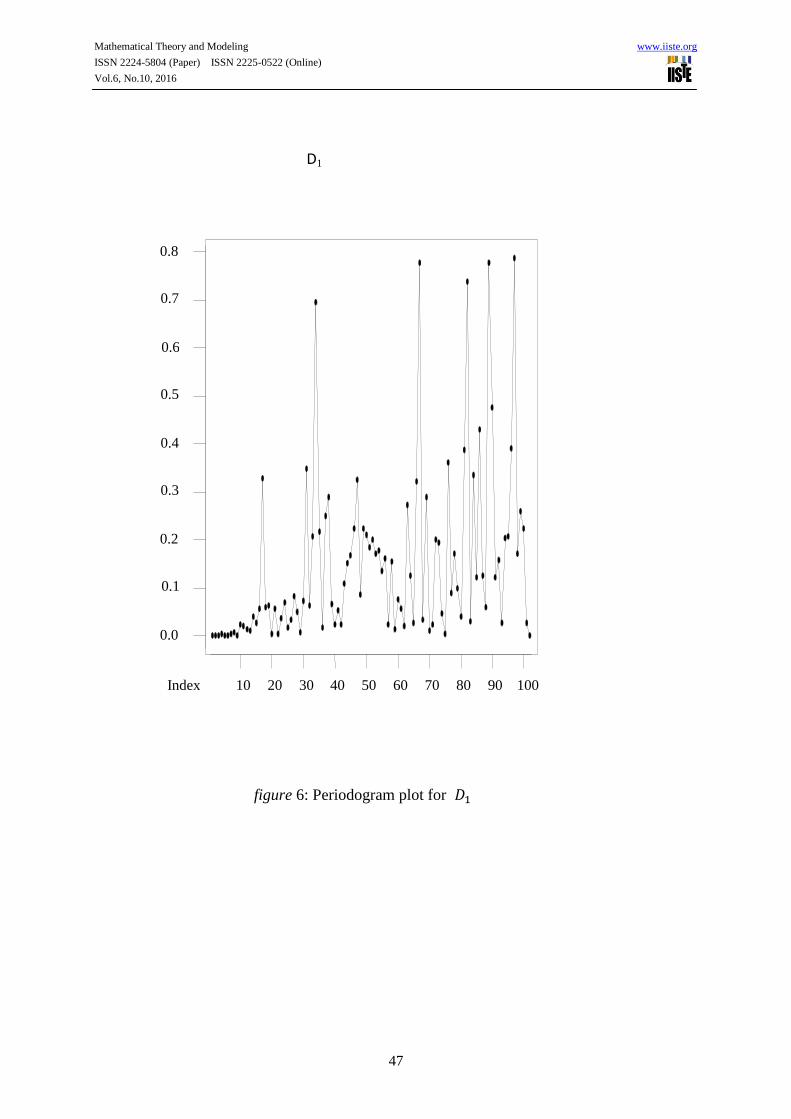
seasonal behaviour and noise. The coefficient at detail one from the periodogram in figure 6

depicts a high frequency noise, while the coefficients at detail three and two captured seasonal

variation of period length 4-16 as seen in fiqure 4 and 5. The coefficients of detail three and

two were added to the coefficients of the smooth series so as to obtain the estimate of {𝑌𝑡}.

This result given in Appendix B is a decomposition of the signal into a range of frequency

scales. The series needed no additional decomposition at this stage because the residual after

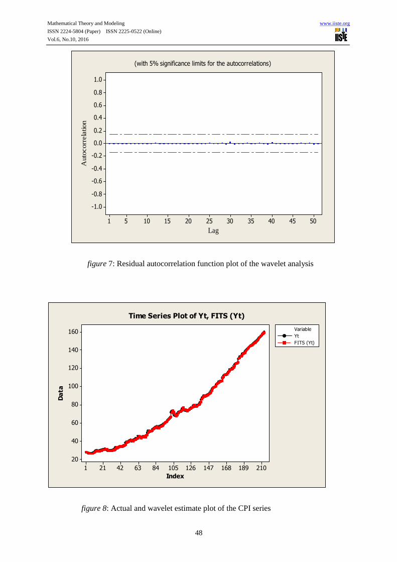
reconstruction was found to be random as shown by the ACF in figure 7.

Hence from (8), the model that reconstructs the series is

�̂�𝑡 = ∑ ∑ 𝑑𝑗,𝑡 + 𝑆𝑗,𝑡203𝑡=0

3𝑗=1 (9)

3.2 Diagonistic Checks

The diagnostic check based on the residuals do not raise any alarm on the validity and

adequacy of the fitted model since the residual ACF plot ( figure 7) does not show any

significant spike above or below the 95 percent confidence interval. This means that the

residuals are consistent with the white noise process; confirming the adequacy of the wavelet

model. Also, the root means square error (RMSE) obtained in fitting the wavelet model is

calculated to be 0.15262. This shows that the strength of the discrepancies between real

values and those estimated by the model is rather very small; indicating a good fit of the

model.

In addition, the actual values of the series {𝑌𝑡} and the values estimated by the wavelet

model (9) are strongly positively correlated (see 𝑌𝑡 and Fits in appendix B). This is also




Vol.6, No.10, 2016

42

confirmed by visual inspection of the actual and estimate plot (figure 8) in which the two

superimposed plots strongly agree and move in the same direction. This further confirms the

adequacy of the model.

4.0 Discussion and Conclusion

As noted in the review, several approaches have been made in the modelling of the

CPI and some good results have been achieved. However, even though some of the fitted

models were found to be adequare; they still suffer some draw backs in taking care of the

trend (smooth) and splitting of the given signal into components that can reflect the evolution

trough time of the signal at a particular time. Besides, the obtained root mean square errors (

7.2587 and 4.2345 ) in Abraham (2014), and Akpanta and Okorie (2015) seem to be

moderately high and should not be considered as the best fit for the CPI series. Contrary to

these approaches, the Wavelet approach has decomposed the series into smooth (trend) (𝑆𝑗,𝑡)

and details (𝑑𝑗,𝑡) by using Haar stationary Wavelet technique. The reconstruction of the (𝑆𝑗,𝑡)

at Multi-resolution three gave the smooth 𝑆3 (figure 9). The residual analysis discussed in

section 3.2 has shown clearly that the wavelet model is adequate and by comparing its root

means square error (0.15262) with others; the wavelet model fits the CPI series better than the

Fourier and SARIMA aproaches noted in the review.




Vol.6, No.10, 2016

43

200180160140120100806040201

160

140

120

100

80

60

40

20

Index

figure 1: Raw data plot of {𝑌𝑡}

50454035302520151051

1.0

0.8

0.6

0.4

0.2

0.0

-0.2

-0.4

-0.6

-0.8

-1.0

Lag

Auto

corr

ela

tion

(with 5% significance limits for the autocorrelations)

figure 2 : Autocorelation plot of second difference of {𝑌𝑡}




Vol.6, No.10, 2016

44

50454035302520151051

1.0

0.8

0.6

0.4

0.2

0.0

-0.2

-0.4

-0.6

-0.8

-1.0

Lag

Part

ial A

uto

corr

ela

tion

(with 5% significance limits for the partial autocorrelations)

figure 3 : Partial Autocorelation plot of second difference of {𝑌𝑡}




Vol.6, No.10, 2016

45

figure 4: Periodogram plot for 𝐷3

100 90 80 70 60 50 40 30 20 10

15

10

5

0

Index

D3




Vol.6, No.10, 2016

46


100 90 80 70 60 50 40 30 20 10

15

10

5

0

Index

D2




Vol.6, No.10, 2016

47


100 90 80 70 60 50 40 30 20 10

0.8

0.7

0.6

0.5

0.4

0.3

0.2

0.1

0.0

Index

D1




Vol.6, No.10, 2016

48

50454035302520151051

1.0

0.8

0.6

0.4

0.2

0.0

-0.2

-0.4

-0.6

-0.8

-1.0

Lag

Auto

corr

ela

tion

(with 5% significance limits for the autocorrelations)

figure 7: Residual autocorrelation function plot of the wavelet analysis

figure 8: Actual and wavelet estimate plot of the CPI series

Index

Da

ta

210189168147126105846342211

160

140

120

100

80

60

40

20

Variable

Yt

FITS (Yt)

Time Series Plot of Yt, FITS (Yt)




Vol.6, No.10, 2016

49

200180160140120100806040201

160

140

120

100

80

60

40

20

0

Index

S3

figure 9: Time Plot for Trend or Smooth 𝑆3

References

Abraham, H. S. (2014). Modeling Nigerian Consumer Price Index Using ARIMA. International Journal of Development Economic and Sustainability. Vol. 5, No. 8, pp. 41-48. ISBN: 0-2234-354-8. Akpanta, A. C. and Okorie I. E. (2015): Time Series Analysis of Consumer Price Index Data

of Nigeria. American Journal of Economics p-ISSN: 2166-4951 e-ISSN: 2166-496x 2015; 5(3): 363-369 doi: 10.5923/j.economics.20150503.08.

Al Wadi, S., Ismail, M. T. and Abdul Karim S. A. (2010): A comparison between Haar Wavelet Transform and Fast Fourier Transform in Analyzing Financial time series Data. Research Journal of Applied Sciences 2010/volume 5/issue: 5/page No:352-360 DOI: 103923/rjasci. 2010 352-360.

Crowdly, P. (2005): An intuitive guide to Wavelet for economics, working paper, Bank of Finland.

Daubechies, I. (1992): Ten Lectures on wavelets. Philadelphia, Pa: Society for industrial and Applied Mathematics, vol. 64, 1992, CBMS-NSF Regional Conference Series in Applied Mathematics.

Gencay, R., Selcuk, F. and Whitcher, B. (2002), An Introduction to Wavelet and other Filtering Methods in Finance and Economics, Academic Press, San Diego.

Mallet, S. G. (2001). A Wavelet tour of signal Processing; Academic Press, New York. ISBN: 0-2142-1314-5

Mehala, N. and Dahiya, R. (2013): A comparative study of Fast Fourier Transform,Short Fourier Transform and the Wavelet techniques for induction Machine Fault Diagnostic Analysis proc. of the 7th Wseas int. conf. on computationalInteligent,Man-Machine Systems and Cybernetics [email protected],[email protected].

Manahanda, P., Kumar, J. and Siddiqi, A. H. (2007): Mathematical methods for modeling price fluctuations of financial time series J. Franklin inst., 344:61-63


mailto:[email protected],[email protected]



Vol.6, No.10, 2016

50

Masset, P. (2008). Analysis of Financial Time-Series using Fourier and WaveletMethods.University of Fribourg, Department of Finance,Bd.Pérolles 90, CH-1700 Fribourg, [email protected].

Mukhopadhyay, S., Dash, D., Mitra, A., Bhattacharya, P. (2013). A comparative study between seasonal wind speed by Fourier and Wavelet analysis. India institute of Science Research Kolkata, Mohanpur campus, nadia-741252, india.

Nachane, M. and Clavel, G. (2014): Forecasting Interest Rates: A Comparative Assessment of Some Second Generation Nonlinear Models.EMail:[email protected] and E-mail:[email protected].

Omekara, C. O.,Ekpenyong, E. J. and Ekerete, M. P. (2013): Modeling the Nigeria Inflation Rates using Periodogram and Fourier Series Analysis: CBN Journal of Applied Statistics Vol. 4 No. 2.

Renaud O., Stark J. L. and Martagh (2004): Wavelet-based Forecasting of Short and Long Memory Time Series http://www.unique.ch/ses/metril.

Yogo, M. (2003): Measuring Business Cycles,Wavelet Analysis of Economic Time Series.Department of Economics, Harvard University. Email:[email protected].

Appendix A

Wavelet Analysis Program Using Matlab

s=consumer price index(CPI)

(swa,swd)=swt(s,1,'db1');

[swa,swd]=swt(s,1,'db1');

whos

Subplot(1 2,1),plot(swa);title('Approximation cfs')

subplot(1,2,2),plot(swd);title('Detail cfs')

A0=iswt(swa,swd,'db1);

err=norm(S-A0)

nulcfs=zeros(size(swa));

A1=iswt(swa,nulcfs,'db1');

D1=iswt(nulcfs,swd,'db1');

subplot(1,2,1),plot(A1);title('Approximation A1')

subplot(1,2,2),plot(D1);title('Detail D1')

[swa,swd]=swt(s,3,'db1);

[swa,swd]= swt(s,3,'db1');

clear A0 A1 D1 err nulcfs

whos

Multilevel decomposition and reconstruction.

kp=0;

for i=1:3

subplot(3,2,kp+1), plot(swa(i,:));

title(['Approx. cfs level ',num2str(i)])

subplot(3,2,kp+2),plot(swd(i,:));

title(['Detail cfs level ',num2str(i)])

kp=kp+2;

end

mzero= zeros(size(swd));

A= mzero;

A(3,:)=iswt(swa,mzero,'db1');

D= mzero;




Vol.6, No.10, 2016

51

for i = 1:3

swcfs = mzero;

swcfs(i,:) = swd(i,:);

D(i,:) = iswt(mzero,swcfs,'db1');

end

A(2,:)=A(3,:) + D(3,:);

A(1,:)=A(2,:) + D(2,:);

kp = 0;

for i = 1:3

subplot(3,2,kp+1), plot(A(i,:));

title(['Approx. level ',num2str(i)])

subplot(3,2,kp+2),plot(D(i,:));

title(['Detail level ',num2str(i)])

kp = kp + 2;

end

[thr,sorh] = ddencmp('den','wv',s);

dswd = wthresh(swd,sorh,thr);

clean = iswt(swa,dswd,'db1');

subplot(2,1,1),plot(s);

title('original signal')

subplot(2,1,2), plot(clean);

title('De-noised signal')

err=norm(s-clean).

Appendix B

Estimates of Consumer Price Index using Wavelet analysis

Yt S3 D3 D2 Fit D1

27.46 22.058 1.8197 3.5919 27.470 -0.010000

26.96 17.964 3.8386 5.1550 26.958 0.002500

26.45 20.461 4.5433 1.5681 26.572 -0.122500

26.43 22.581 3.9723 -0.1238 26.430 0.000000

26.41 24.338 2.1392 -0.0750 26.403 0.007500

26.36 25.730 0.8041 -0.1369 26.398 -0.037500

26.46 26.749 -0.0311 -0.1856 26.533 -0.072500

26.85 27.392 -0.3456 -0.1338 26.912 -0.062500

27.49 27.653 -0.1333 -0.1150 27.405 0.085000

27.79 27.947 0.1034 -0.0875 27.962 -0.172500

28.78 28.263 0.2928 0.1813 28.738 0.042500

29.6 28.567 0.3542 0.4413 29.363 0.237500

29.47 28.835 0.2606 0.2494 29.345 0.125000

28.84 29.074 0.0780 -0.1544 28.997 -0.157500

28.84 29.307 -0.0839 -0.2681 28.955 -0.115000

29.3 29.539 -0.1598 -0.1294 29.250 0.050000

29.56 29.756 -0.1275 0.0088 29.637 -0.077500

30.13 29.943 -0.0013 0.0781 30.020 0.110000




Vol.6, No.10, 2016

52

30.26 30.083 0.1423 0.0594 30.285 -0.025000

30.49 30.185 0.2922 0.0006 30.477 0.012500

30.67 30.253 0.4184 0.0231 30.695 -0.025000

30.95 30.287 0.4497 0.1956 30.933 0.017500

31.16 30.263 0.3953 0.3537 31.012 0.147500

30.78 30.181 0.2244 0.1994 30.605 0.175000

29.7 30.065 -0.0234 -0.1262 29.915 -0.215000

29.48 29.961 -0.2278 -0.2531 29.480 0.000000

29.26 29.901 -0.3902 -0.1881 29.323 -0.062500

29.29 29.915 -0.4777 -0.0694 29.368 -0.077500

29.63 30.002 -0.4980 -0.0219 29.483 0.147500

29.38 30.168 -0.5277 -0.1081 29.532 -0.152500

29.74 30.432 -0.5088 -0.1931 29.730 0.010000

30.06 30.788 -0.4095 -0.2487 30.130 -0.070000

30.66 31.214 -0.2548 -0.2094 30.750 -0.090000

31.62

32.99

31.676

32.151

-0.0175

0.2198

0.0637

0.2369

31.723

32.608

-0.102500

0.382500

32.83 32.603 0.3561 0.1013 33.060 -0.230000

33.59 33.041 0.3923 0.0838 33.518 0.072500

34.06 33.484 0.2631 0.2456 33.993 0.067500

34.26 33.928 0.0105 0.1537 34.092 0.167500

33.79 34.365 -0.2508 -0.1719 33.942 -0.152500

33.93 34.826 -0.4875 -0.2862 34.053 -0.122500

34.56 35.329 -0.5466 -0.2025 34.580 -0.020000

35.27 35.880 -0.4148 -0.3075 35.157 0.112500

35.53 36.483 -0.2097 -0.2456 36.028 -0.497500

37.78 37.108 0.0853 0.2988 37.493 0.287500

38.88 37.696 0.3084 0.4531 38.458 0.422500

38.29 38.241 0.4098 -0.0181 38.633 -0.342500

39.07 38.775 0.4961 -0.1956 39.075 -0.005000

39.87 39.267 0.4406 0.1375 39.845 0.025000

40.57 39.709 0.2834 0.4825 40.475 0.095000

40.89 40.093 0.1041 0.3106 40.508 0.382500

39.68 40.421 -0.1375 -0.3388 39.945 -0.265000

39.53 40.770 -0.3116 -0.5313 39.928 -0.397500

40.97 41.174 -0.3270 -0.0769 40.770 0.200000

41.61 41.602 -0.2748 0.1456 41.473 0.137500

41.7 42.001 -0.1537 0.0556 41.902 -0.202500

42.6 42.402 0.0539 -0.0212 42.435 0.165000

42.84 42.789 0.2208 -0.1969 42.813 0.027500

42.97 43.178 0.3783 -0.0738 43.482 -0.512500

45.15 43.561 0.4641 0.4850 44.510 0.640000




Vol.6, No.10, 2016

53

44.77 43.843 0.3953 0.5869 44.825 -0.055000

44.61 44.064 0.2248 -0.0213 44.267 0.342500

43.08 44.259 0.0139 -0.4525 43.820 -0.740000

44.51 44.523 -0.1756 -0.2369 44.110 0.400000

44.34 44.844 -0.4050 0.1863 44.625 -0.285000

45.31 45.232 -0.5628 0.2313 44.900 0.410000

44.64 45.698 -0.7648 -0.2481 44.685 -0.045000

44.15 46.273 -0.9016 -0.6063 44.765 -0.615000

46.12 47.017 -0.7575 -0.5219 45.737 0.382500

46.56 47.877 -0.5769 -0.2450 47.055 -0.495000

48.98 48.845 -0.1923 0.2244 48.877 0.102500

50.99 49.827 0.1745 0.3231 50.325 0.665000

50.34 50.756 0.3541 0.0100 51.120 -0.780000

52.81 51.651 0.5875 0.0637 52.303 0.507500

53.25 52.476 0.6669 0.1800 53.323 -0.072500

53.98 53.207 0.7278 0.0906 54.025 -0.045000

54.89 53.822 0.7222 0.2606 54.805 0.085000

55.46 54.332 0.4955 0.5575 55.385 0.075000

55.73 54.737 0.2277 0.2806 55.245 0.485000

54.06 55.086 -0.1308 -0.4406 54.515 -0.455000

54.21 55.472 -0.3816 -0.5275 54.563 -0.352500

55.77 55.893 -0.4584 -0.0269 55.407 0.362500

55.88 56.348 -0.4727 0.1144 55.990 -0.110000

56.43 56.856 -0.3556 -0.0925 56.407 0.022500

56.89 57.425 -0.2633 -0.2019 56.960 -0.070000

57.63 58.074 -0.1986 -0.0975 57.777 -0.147500

58.96 58.806 -0.1281 0.0600 58.738 0.222500

59.4 59.601 -0.1344 0.0706 59.538 -0.137500

60.39 60.498 -0.2106 -0.0119 60.275 0.115000

60.92 61.493 -0.3833 -0.0950 61.015 -0.095000

61.83 62.576 -0.5842 -0.1319 61.860 -0.030000

62.86 63.693 -0.7212 -0.0988 62.873 -0.012500

63.94 64.795 -0.5405 -0.2819 63.972 -0.032500

65.15 65.841 0.0375 -0.7531 65.125 0.025000

66.26 66.805 0.8384 -0.4306 67.213 -0.952500

71.18 67.690 1.6705 1.0294 70.390 0.790000

72.94 68.380 2.0039 1.7913 72.175 0.765000

71.64 68.858 1.6380 1.0413 71.538 0.102500

69.93 69.175 0.7655 0.0319 69.972 -0.042500

68.39 69.396 -0.3278 -0.5481 68.520 -0.130000

67.37 69.607 -1.1097 -0.8550 67.642 -0.272500

67.44 69.895 -1.3320 -0.8675 67.695 -0.255000




Vol.6, No.10, 2016

54

68.53 70.282 -1.1055 -0.4438 68.733 -0.202500

70.43 70.722 -0.6355 0.2531 70.340 0.090000

71.97 71.226 -0.1756 0.5475 71.597 0.372500

72.02 71.762 0.1947 0.0156 71.972 0.047500

71.88 72.305 0.5284 -0.5612 72.272 -0.392500

73.31 72.841 0.8061 -0.1050 73.543 -0.232500

75.67 73.313 0.9917 0.8875 75.193 0.477500

76.12 73.645 0.9273 0.9600 75.533 0.587500

74.22 73.830 0.5480 0.1850 74.563 -0.342500

73.69 73.961 0.0230 -0.3012 73.682 0.007500

73.13 74.091 -0.4975 -0.4006 73.192 -0.062500

72.82 74.292 -0.8131 -0.4413 73.037 -0.217500

73.38 74.581 -0.8517 -0.3044 73.425 -0.045000

74.12 74.913 -0.6847 -0.0706 74.158 -0.037500

75.01 75.285 -0.4134 0.0038 74.875 0.135000

75.36 75.713 -0.0750 -0.0775 75.560 -0.200000

76.51 76.210 0.2781 -0.1781 76.310 0.200000

76.86 76.715 0.4964 0.0613 77.272 -0.412500

78.86 77.218 0.5856 0.6544 78.457 0.402500

79.25 77.666 0.4302 0.6437 78.740 0.510000

77.6 78.068 0.0667 -0.1469 77.987 -0.387500

77.5 78.530 -0.3214 -0.5763 77.633 -0.132500

77.93 79.097 -0.7048 -0.2875 78.105 -0.175000

79.06 79.786 -0.9512 -0.0044 78.830 0.230000

79.27 80.580 -1.0667 -0.1412 79.372 -0.102500

79.89 81.485 -0.9930 -0.4469 80.045 -0.155000

81.13 82.484 -0.6828 -0.5963 81.205 -0.075000

82.67 83.581 -0.2036 -0.3300 83.047 -0.377500

85.72 84.742 0.4184 0.2625 85.422 0.297500

87.58 85.855 0.8919 0.6231 87.370 0.210000

88.6 86.870 1.0713 0.6487 88.590 0.010000

89.58 87.770 0.9652 0.4650 89.200 0.380000

89.04 88.568 0.5645 0.0300 89.163 -0.122500

88.99 89.312 0.1228 -0.2644 89.170 -0.180000

89.66 90.043 -0.2464 -0.1812 89.615 0.045000

90.15 90.777 -0.5450 -0.0344 90.198 -0.047500

90.83 91.531 -0.6838 -0.0544 90.792 0.037500

91.36 92.338 -0.7070 -0.2681 91.362 -0.002500

91.9 93.221 -0.5838 -0.4494 92.188 -0.287500

93.59 94.212 -0.3034 -0.3087 93.600 -0.010000




Vol.6, No.10, 2016

55

95.32 95.290 0.0061 0.0837 95.380 -0.060000

97.29 96.422 0.2331 0.4175 97.073 0.217500

98.39 97.543 0.2697 0.4250 98.238 0.152500

98.88 98.642 0.1575 0.0756 98.875 0.005000

99.35 99.711 0.0105 -0.3262 99.395 -0.045000

100 100.794 -0.0467 -0.3719 100.375 -0.375000

102.15 101.897 0.0127 -0.0519 101.857 0.292500

103.13 102.992 0.0684 0.3025 103.363 -0.232500

105.04 104.082 0.0225 0.4231 104.527 0.512500

104.9 105.140 -0.1147 0.1144 105.140 -0.240000

105.72 106.203 -0.2472 -0.4506 105.505 0.215000

105.68 107.284 -0.2367 -0.5869 106.460 -0.780000

108.76 108.413 -0.0155 -0.1125 108.285 0.475000

109.94 109.519 0.2438 0.3644 110.128 -0.187500

111.87 110.601 0.3895 0.5244 111.515 0.355000

112.38 111.621 0.3592 0.3569 112.338 0.042500

112.72 112.596 0.1561 -0.1050 112.647 0.072500

112.77 113.563 -0.0378 -0.4056 113.120 -0.350000

114.22 114.525 -0.0572 -0.2675 114.200 0.020000

115.59 115.479 -0.0014 0.0475 115.525 0.065000

116.7 116.410 0.0734 0.3394 116.823 -0.122500

118.3 117.340 0.0995 0.3006 117.740 0.560000

117.66 118.239 -0.0655 -0.0856 118.087 -0.427500

118.73 119.177 -0.1967 -0.2275 118.753 -0.022500

119.89 120.195 -0.2747 -0.2250 119.695 0.195000

120.27 121.267 -0.3122 -0.2800 120.675 -0.405000

122.27 122.416 -0.2750 0.0619 122.203 0.067500

124 123.603 -0.3334 0.4481 123.718 0.282500

124.6 124.812 -0.3561 0.0069 124.463 0.137500

124.65 126.065 -0.3456 -0.7519 124.968 -0.317500

125.97 127.391 -0.1830 -0.5131 126.695 -0.725000

130.19 128.753 0.1395 0.3325 129.225 0.965000

130.55 130.057 0.3586 0.5644 130.980 -0.430000

132.63 131.329 0.5370 0.2862 132.153 0.477500

132.8 132.524 0.4839 0.0000 133.008 -0.207500

133.8 133.683 0.2750 -0.0225 133.935 -0.135000

135.34 134.815 0.1258 0.0938 135.035 0.305000

135.66 135.900 -0.0353 -0.0575 135.808 -0.147500

136.57 136.944 -0.0725 -0.1838 136.688 -0.117500

137.95 137.950 -0.0280 -0.0125 137.910 0.040000

139.17 138.958 0.0053 0.1112 139.075 0.095000

140.01 139.949 0.0564 0.0575 140.063 -0.052500




Vol.6, No.10, 2016

56

141.06 140.940 0.0855 -0.0075 141.017 0.042500

141.94 141.907 0.0925 -0.0144 141.985 -0.045000

143 142.856 0.1092 0.0250 142.990 0.010000

144.02 143.794 0.1250 0.0456 143.965 0.055000

144.82 144.713 0.1239 0.0256 144.862 -0.042500

145.79 145.619 0.0869 0.0562 145.762 0.027500

146.65 146.520 0.0094 0.1031 146.633 0.017500

147.44 147.419 -0.0853 0.0013 147.335 0.105000

147.81 148.324 -0.1706 -0.1631 147.990 -0.180000

148.9 149.254 -0.1883 -0.1631 148.902 -0.002500

150 150.208 -0.1519 -0.0562 150.000

151.122

0.000000

151.1 151.188 -0.0983 0.0331 -0.022500

152.29 152.190 -0.0383 0.0831 152.235 0.055000

153.26 150.696 2.4817 0.0319 153.210 0.050000

154.03 146.691 7.4994 -0.0531 154.138 -0.107500

155.23 140.164 15.0741 -0.0681 155.170 0.060000

156.19 131.090 25.2141 -0.0513 156.253 -0.062500

157.4 119.444 27.9198 10.0388 157.403 -0.002500

158.62 105.206 23.1216 30.2450 158.573 0.047500

159.65 128.355 10.7358 20.3894 159.480 0.170000


Another Look at the Consumer Price Index - A wavelet Approach

Documents

Transcript of Another Look at the Consumer Price Index - A wavelet Approach