Anomaly Detection for an E-commerce Pricing SystemJagdish Ramakrishnan

Walmart LabsSan Bruno, CA

jramakrishnan@walmartlabs.com

Elham ShaabaniWalmart LabsSan Bruno, CA

Elham.Shaabani@walmartlabs.com

Chao LiWalmart LabsSan Bruno, CA

CLi0@walmart.com

Mátyás A. SustikWalmart LabsSan Bruno, CA

MSustik@walmartlabs.com

ABSTRACTOnline retailers execute a very large number of price updates whencompared to brick-and-mortar stores. Even a few mis-priced itemscan have a significant business impact and result in a loss of cus-tomer trust. Early detection of anomalies in an automated real-timefashion is an important part of such a pricing system. In this pa-per, we describe unsupervised and supervised anomaly detectionapproaches we developed and deployed for a large-scale onlinepricing system at Walmart. Our system detects anomalies bothin batch and real-time streaming settings, and the items flaggedare reviewed and actioned based on priority and business impact.We found that having the right architecture design was criticalto facilitate model performance at scale, and business impact andspeed were important factors influencing model selection, param-eter choice, and prioritization in a production environment for alarge-scale system. We conducted analyses on the performance ofvarious approaches on a test set using real-world retail data andfully deployed our approach into production. We found that ourapproach was able to detect the most important anomalies withhigh precision.

1 INTRODUCTIONPricing plays a critical role in every consumer’s purchase decision.With the rapid evolution of e-commerce and a growing need tooffer consumers a seamless omni-channel (e.g., store and online)experience, it is becoming increasingly important to calculate andupdate prices of merchandise online dynamically to stay ahead ofthe competition. AtWalmart, the online pricing algorithm is respon-sible for calculating the most suitable price for tens of millions ofproducts on Walmart.com. The algorithm takes both external data,such as competitor prices, and internal data, such as distributorcosts, marketplace prices, and Walmart store prices, as inputs tocalculate the final price that meets business needs (e.g., top lineand bottom line objectives). The calculation is carried out in real-time with large amounts of data, which includes more than tensof millions of item cost data points and marketplace data pointsper day at Walmart. Many of the data sources are prone to dataerrors and some of them are out of the company’s control. Dataerrors could lead to incorrect price calculations that can result inprofit and revenue losses. For example, an incorrectly entered costupdate for an item could drive a corresponding change for the priceof the item. Note that an incorrect price of a digitally distributed

product such as a code for a computer game could trigger signifi-cant financial losses within minutes without recourse. In addition,incorrect prices could hurt Walmart’s EDLP (Every Day Low Price)value proposition, expose the company to a legal risk related toprice agreements with manufacturers, and erode customer trust.

One approach to anomaly detection is to detect an anomaly if anitem’s price is more than a few standard deviations from its averagehistorical price. However, given that large fluctuations in priceare common in an online setting, this approach results in manyfalse positives. Furthermore, not only do we want to detect priceanomalies, we also want to identify and correct data errors thatare the root cause of a price anomaly. This includes item attributessuch as cost and reference prices from other channels.

To address this challenge, we developed a machine learning-based anomaly detection system that uses both supervised andunsupervised models. We used many features including prices fromother channels, binary features, categorical features, and their trans-formations. We deployed the system into production in both a batchand streaming setting and implemented a review process to gener-ate labeled data in collaboration with an internal operations team.Although the system was built for detecting pricing anomalies, webelieve that the insights learned from model training, testing, andtuning, system and architecture design, and prioritization frame-work are relevant in any application that requires real-time identi-fication and correction of data quality issues for large amounts ofdata.

Compared to previously published work on anomaly detection,the novel contributions of this paper are:

• An anomaly detection approach for a large-scale on-line pricing system - While there are numerous applica-tions of anomaly detection [34], including intrusion detec-tion, fraud detection, and sensor networks, there are rela-tively few references on anomaly detection in a retail setting.To the best of our knowledge, this is the first paper document-ing methodologies, model performance, and system archi-tecture on anomaly detection for a large scale e-commercepricing system.

• Features and transformations for improvingmodel per-formance - The choice of features played an important rolein model performance. We used a variety of features as in-puts to our models, including price-based, binary, categorical,

arX

iv:1

902.

0956

6v5

[cs

.LG

] 1

Jun

201

9

, , Jagdish Ramakrishnan, Elham Shaabani, Chao Li, and Mátyás A. Sustik

hierarchical, and feature transformations. We found that log-based feature transformations were especially useful for ourGaussian-based and autoencoder models.

• An approach to explain anomalies - While our proposedGaussian Naive Bayes baseline model does not perform aswell as the other sophisticated models, it served as the basisfor our approach to explain anomalies. We used the scoresfrom the model together with rule-based logic to providereasonable explanations for why items were detected asanomalies. The use of explanations played an important rolein directing human review of the items.

• Aprioritization schemebased onbusiness impact - Dueto the large number of potential anomalies, we needed toprioritize and focus our attention on the ones that had thehighest business impact. This prioritization allowed us toselect the most important anomalies for human review givena fixed budget of items that could be reviewed in a givenperiod of time.

• Supervised and unsupervised models for anomaly de-tection - Unsupervised approaches formed the basis of ourinitial models used in production because we had very fewand insufficient labeled anomaly instances. As more itemswere reviewed, we increased our anomaly-labeled instancesand moved to supervised approaches that had superior per-formance. Moving forward, we believe a combination of bothsupervised and unsupervised models will work well by usingexisting labeled anomalies efficiently, and at the same time,using models of normal instances to detect anomalies evenwhen they are very different from those in our labeled set.

• An architecture for model performance at scale - Thebest performing model may not be the most effective model.We had to balance model performance and speed in a pro-duction environment to select the most effective model forour use case of real-time anomaly detection. For example,in our streaming setting, we used the baseline model ratherthan much better performing models because speed was acritical factor. In the batch setting, however, model perfor-mance played an important role, and we used the highestperforming models.

2 RELATEDWORKThere is a significant amount of literature on anomaly detectionmethods, including density-based [14, 20], quantile-based [31, 35],neighborhood-based [10, 22], and projection-basedmethods [25, 28].A majority of papers focus on unsupervised methods, althoughthere is representative work on both semi-supervised and super-vised anomaly detection approaches [16]. Tree-based methods, suchas Isolation Forest [25], are especially attractive because they scalewell with large datasets and have fast prediction times. Further-more, they work well with diverse features, such as discrete andcontinuous, and the features do not need to be normalized. Forother methods such as one-class SVMs [31] and k-NN [7], however,training time and/or memory requirements can rapidly increasewith the size of the training data.

There has been recent interest in neural network based modelsfor anomaly detection, including autoencoders [38] and generative

models such as GANs [37]. In [38], the authors propose deep struc-tured energy-based models, where the energy function is definedas the output of a neural network. One example of such a model isan autoencoder where the anomaly score is the sum of the squarederrors between the input and the output. We evaluate such an au-toencoder model in this paper and compare its performance withother models.

Much of the literature also focuses on time-series anomaly de-tection approaches [6, 18, 32, 40]. There are three main classes ofanomalies: contextual anomalies, anomalous subsequences, andanomalous time-series [19]. Contextual anomalies are single obser-vations at a particular point in time that are significantly differentfrom their expected value. Anomalous subsequences are subse-quences within a time series that differ from other parts of theseries. And, anomalous time-series refers to time-series that differfrom a collection of time series. In this paper, we are mainly focusedon contextual anomalies because we are interested in whether anitem is an anomaly at a particular point in time.

The use of anomaly detection methods in production systems isprevalent among large technology companies, including Yahoo [24],Google [32], Facebook [23], LinkedIn [4], Uber [40], and Twitter [3,36]. While there is some work on anomaly detection in retail [29],to the best of our knowledge, there does not seem to be referenceson anomaly detection for a large-scale pricing system as we haveconsidered in this paper. There are blog posts by companies suchas Anodot [8], but they do not describe models in detail specific tothe pricing context.

3 METHODOLOGYIn this section, we introduce the proposed anomaly detection systemfor Walmart’s online pricing system. We first describe the featuresand their transformations that we used for our models. Next, weintroduce the unsupervised and supervised models that we used.Finally, we describe the overall process and system architecture ofthe deployed models.

3.1 FeaturesWe describe the various types of features that we extracted for ourproblem. Let x represent the feature vector, where the ith featureis represented by xi . Depending on the model we use, the set offeatures may change, but we will make it clear exactly which set offeatures we are using.

Price-based features. In our data, we identify price-based fea-tures as those that have some notion of a price point. The mostobvious ones are the current price, competitor prices, and pricesfrom other channels such as store prices, but cost is also an exampleof a price-based feature as it is relatable to the price of an item. Wedenote the set of indices of the raw price-based features by P, i.e.,xi is a raw price-based feature if i ∈ P. We also use time seriesbased features, whose indices are represented by the set T , such asthe average of the historical prices, its standard deviation, and thepercentage price swing from yesterday’s price.

Binary, categorical, and other numerical features. We havebinary features such as whether an item is part of a marketing pro-motion that impacts pricing or is part of a bundle. We represent theset of indices of binary features as B. For categorical features, we

Anomaly Detection for an E-commerce Pricing System , ,

have data such as the type of promotion and the type of pricing algo-rithm we use. We convert the categorical features into binary formfor modeling purposes. The set of indices for categorical featuresis represented by C. Other numerical features, whose indices werepresent by the set O, include inventory, average customer ratingof the item, and number of units in the item for say a multi-packitem.

Hierarchical features. Additionally, we also have hierarchi-cal based features, i.e., sub-category, category, department, super-department, and division to which an item belongs. Higher levelsof hierarchy contain subsets of the lower levels, e.g., multiple sub-categories are part of a category. Items within a particular hierarchylevel may exhibit different characteristics than others. For example,the electronics category may be selling products at a lower marginthan the jewelry category. Each hierarchy feature is categoricaland represented by an integer. We denote the set of indices of hier-archical features asH . A one-hot encoding of all the hierarchicalfeatures can result in a very large number of features; this can bechallenging to incorporate in models. For some models, we chooseto use a one hot encoding of only a single hierarchy feature, e.g.,the department level. We describe this in more detail when weintroduce models in Sections 3.2 and 3.4.

Transformations of price-based features. We use a varietyof feature transformations as inputs for our models. Since the priceand cost features come up often in our transformation, we usethe notation xp and xc respectively to refer to them. One set oftransformations we use are features that indicate how far the priceis from the cost of the item. These include differences

xi − xc , i ∈ P, xi , xc

and marginsxi − xcxc

, i ∈ P, xi , xc

with respect to the raw price-based features. Similarly, the same setof the above transformations can be applied using xp in place ofxc , where i is over all elements in P except xc and xp . We refer toall of the above transformations with respect to cost and price asprice transformed features and represent the full set of indices forthese features as PT .

Next, we discuss log transformed price features. For somemodelssuch as the autoencoder, we found that log based transformationsare helpful in improving performance and speeding up training.This type of behavior for neural network models has been reportedpreviously [17]. For ease in explanation, we denote the set A to bethe indices of the six features that are the most important features inour pricing algorithm, e.g., price, cost, average historical price. Ourbaseline model makes use of these features. Using these features,we found log based transformations of the following form helpedmake the feature look more Gaussian:

log(xi + c1xc + c1

)+ c2, i ∈ A, xi , xc , (1)

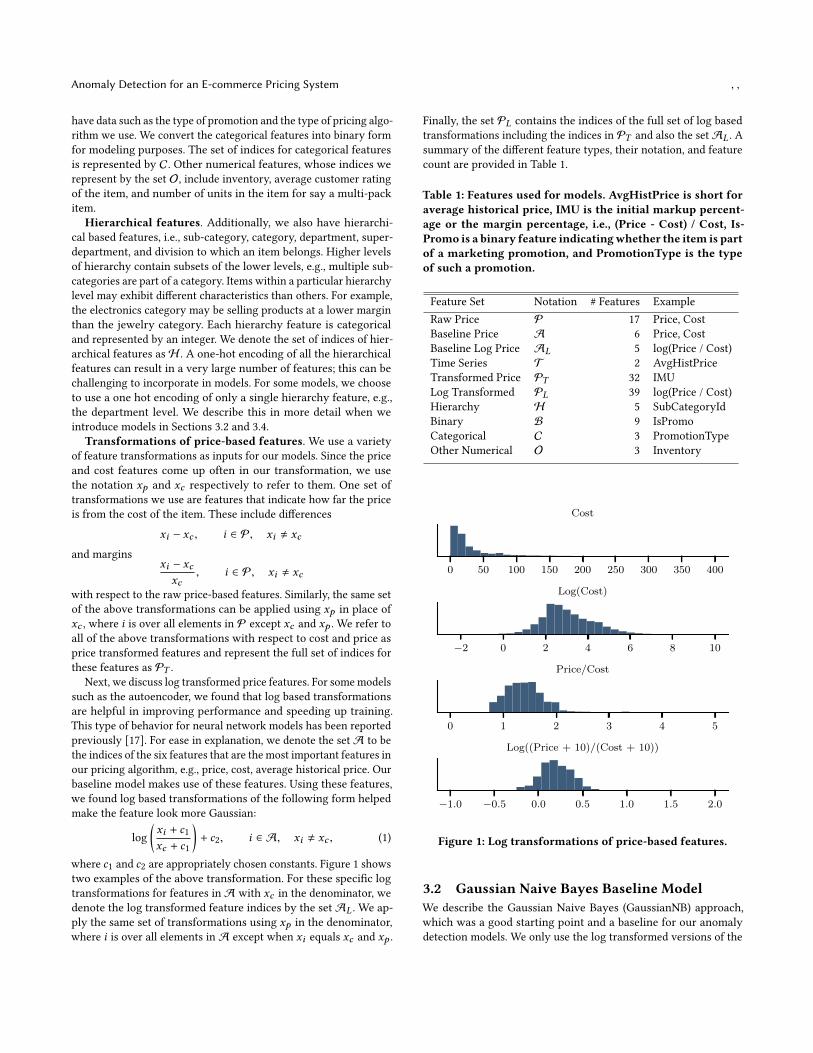
where c1 and c2 are appropriately chosen constants. Figure 1 showstwo examples of the above transformation. For these specific logtransformations for features in A with xc in the denominator, wedenote the log transformed feature indices by the set AL . We ap-ply the same set of transformations using xp in the denominator,where i is over all elements in A except when xi equals xc and xp .

Finally, the set PL contains the indices of the full set of log basedtransformations including the indices in PT and also the set AL . Asummary of the different feature types, their notation, and featurecount are provided in Table 1.

Table 1: Features used for models. AvgHistPrice is short foraverage historical price, IMU is the initial markup percent-age or the margin percentage, i.e., (Price - Cost) / Cost, Is-Promo is a binary feature indicatingwhether the item is partof a marketing promotion, and PromotionType is the typeof such a promotion.

Feature Set Notation # Features ExampleRaw Price P 17 Price, CostBaseline Price A 6 Price, CostBaseline Log Price AL 5 log(Price / Cost)Time Series T 2 AvgHistPriceTransformed Price PT 32 IMULog Transformed PL 39 log(Price / Cost)Hierarchy H 5 SubCategoryIdBinary B 9 IsPromoCategorical C 3 PromotionTypeOther Numerical O 3 Inventory

0 50 100 150 200 250 300 350 400

Cost

−2 0 2 4 6 8 10

Log(Cost)

0 1 2 3 4 5

Price/Cost

−1.0 −0.5 0.0 0.5 1.0 1.5 2.0

Log((Price + 10)/(Cost + 10))

Figure 1: Log transformations of price-based features.

3.2 Gaussian Naive Bayes Baseline ModelWe describe the Gaussian Naive Bayes (GaussianNB) approach,which was a good starting point and a baseline for our anomalydetection models. We only use the log transformed versions of the

, , Jagdish Ramakrishnan, Elham Shaabani, Chao Li, and Mátyás A. Sustik

main features used in our pricing algorithm, whose indices aredescribed by the set AL . The basic idea of density-based anomalydetection models are that we build a probability distribution p(x)of the normal class and if the density is below some threshold, weclassify as an anomaly. The assumptions for GaussianNB are thatthe features are conditionally independent of the normal class, andthe likelihood of the features are Gaussian. This would mean wehave

p(x) =∏i ∈AL

p(xi ), (2)

where the p(xi ) is the likelihood corresponding to the feature xi ,and

p(xi ) =1√2πσ 2

i

exp−(xi − µi )2

2σ 2i

, (3)

where the µi and σi are the mean and the standard deviation ofthe ith feature, respectively. The choice of the threshold can thenbe selected from a validation set to get an ideal tradeoff betweenprecision and recall.

Since items are part of a particular hierarchy level, e.g., a category,we can have a different model for each hierarchy level. Fittingmodels at a very low hierarchy level, e.g., at a subcategory level,have low bias but may overfit on the training set. On the otherhand, fitting models at a higher hierarchy level may have a higherbias and underfit. We will explore the tradeoff between the varioussetups in the numerical experiments section.

3.3 Explaining AnomaliesWhile having the ability to predict anomalies is important, it isequally important to be able to guide a human reviewer to the causeof the anomalies. Given that there could be many possible reasonsfor an anomaly, we need to direct a reviewer to possible suspectedissues. The advantage of the simple GaussianNB model is that wecan use it to infer possible suspected issues. As before, we use onlythe feature indices represented by AL . We use transformationsof form (1), where the Cost feature xc is used in the denominatorand all other features are used in the numerator. This results in atotal of five features, each of which can give some indication of anissue with either the numerator feature or the denominator featurexc . As mentioned earlier, using these log transformations makesfeatures look more Gaussian, which the GaussianNB model wouldmodel well. These features provide information about how eachprice-based feature compares to the Cost of the item.

With GaussianNB, each feature can be assigned an anomalyscore. To obtain the anomaly score, we take the log transformationof the density and multiply the resulting quantity by a constant.Now, from equations (2) and (3), it can be seen that the anomalyscore A(x) is

A(x) =∑

{i ∈AL :Ai (xi ),NaN}Ai (xi ) =

∑i ∈AL

(xi − µi )2

σ 2i

,

where Ai (xi ) is the anomaly score associated with the ith feature,and we define Ai (xi ) to equal to NaN whenever the numeratorfeature in (1) is missing. Now, we can choose a threshold ϵ so thatif A(x) is above ϵ we would predict an anomaly. We define L[i]for i ∈ AL to be the name of the numerator feature associated

with the ith feature, e.g., for log((Price + c1)/(Cost + c1)) + c2 itwould be "Price." Given the anomaly scores and their associatednames, we would like to output a list of suspected issues, whichwe represent as S(x). The detailed pseudocode and logic of thealgorithm is provided in the supplemental Section A.4.

3.4 Beyond the Baseline Model.We use four other approaches beyond the baseline GaussianNBmodel: Isolation Forest [25], Autoencoder [5], Random Forest (RF) [9],andGradient BoostingMachine (GBM) [13].We also tried neighborhood-based approaches such as k-NN [7], LOF [10], Fast ABOD [22] andquantile-based methods such as one-class SVMs [30]; however,their training time or prediction time were too long for our scale.Isolation Forest and Autoencoder are unsupervised approaches,while RF and GBM are supervised approaches. We found tree-basedapproaches, i.e., Isolation Forest, RF, and GBM provided good per-formance and prediction times as we will see in the experimentssection. For these approaches, we used the features from Table 1without any normalization. For the few categorical features, weused one-hot encoded features, and for the hierarchical features, weleft them as label encoded. The Autoencoder approach, on the otherhand, required normalization and had much better performancewhenwe used log transformed features. Further details are providedin the supplemental Section A.2. We used the sum of squared errorsof the input vector and output vector as the anomaly score for theAutoencoder approach. For Isolation Forest, the anomaly score isthe average path lengths of the tree. The supervised tree-based ap-proaches used the probability of anomaly prediction as an anomalyscore. Table 2 summarizes the details of the various models and thenumber of features that they use. Note the Autoencoder approachuses fewer features than the tree-based models because it only useslog transformed features.

Table 2: Models.

Approach Type # FeaturesGaussianNB Unsupervised 5Isolation Forest Unsupervised 121Autoencoder Unsupervised 89GBM Supervised 121RF Supervised 121

3.5 Threshold SelectionFor all the approaches, we vary the threshold ϵ and select theone that maximizes the standard F1 score given by 2 precision·recall

precision+recall .We use cross-validation on the test set; we predict for each foldusing the threshold selected from maximizing the F1 score fromthe remaining folds. An alternative approach that we use in ourproduction system is to choose the threshold that maximizes therecall at a minimum precision level, e.g., 0.80.

3.6 Prioritization Based on Business ImpactWith limited resources in investigating and fixing every anomaly,we needed to prioritize anomalies based on estimated business

Anomaly Detection for an E-commerce Pricing System , ,

impact, or potential loss for Walmart, which we define as

business_impact = max{profit_loss, foregone_revenue}.Here, we assume profit_loss to be loss caused by an incorrect lowprice while foregone_revenue to be loss as a result of an incorrecthigh price. Given that there is no single data source to calculatebusiness_impact with 100% accuracy, we decided to estimate thesequantities by using

profit_loss = maxi

{xi − xp } × Inventory, i ∈ A, xi , xp

and

foregone_revenue = mini{xi } × Inventory, i ∈ A,

where the max and the min above are taken over the features thatare not missing, i.e., not equal to NaN. We then prioritize anomaliesbased on business_impact.

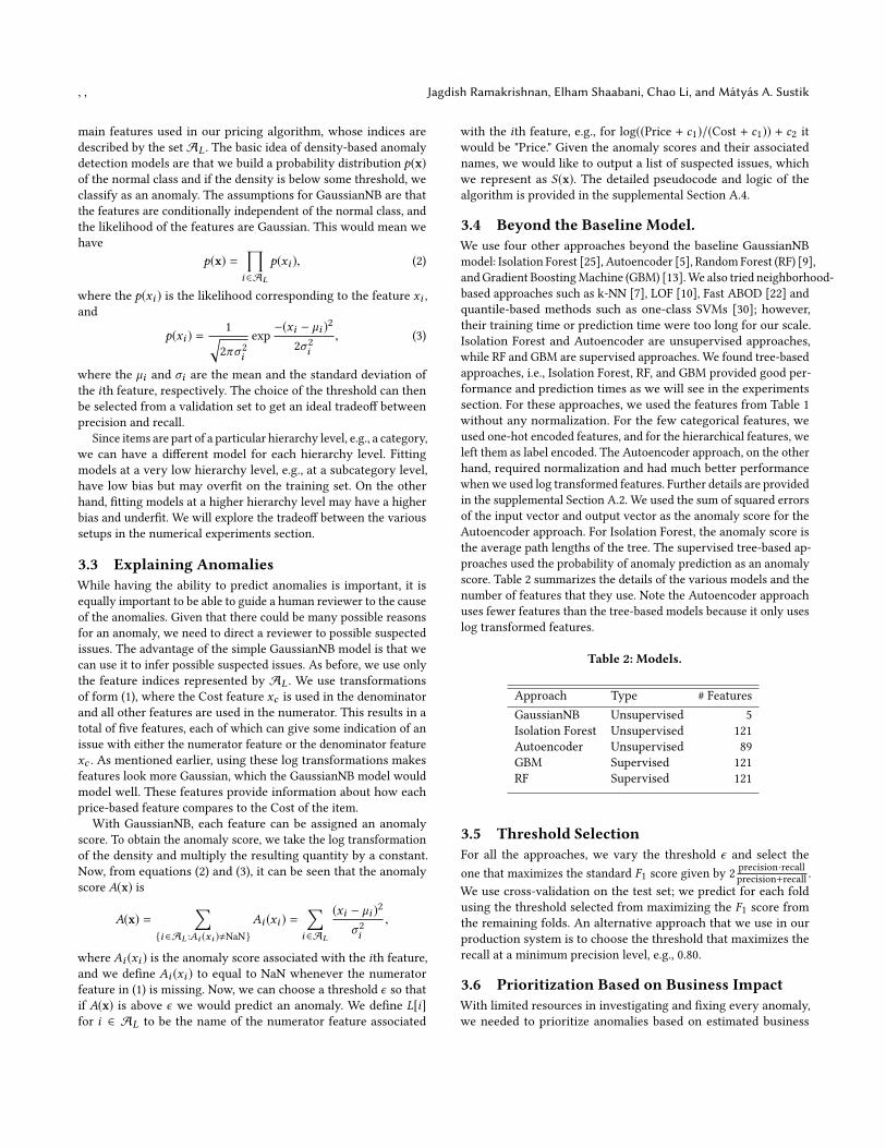
3.7 System ArchitectureThe overall system consists of detection, prioritization, investiga-tion, correction, and model learning, as shown in Figure 2. Basedon more than 1M daily price updates and 100K cost updates, ouranomaly detection models (e.g., GaussianNB, RF) predict anomaliesand prioritize them based on business impact. The most severeanomalies that have high business impact are sent to a manualreview team that has a capacity to review a fixed number anom-alies daily. The reviewed anomalies are appropriately channeled tocategory specialists who correct the problem appropriately. Finally,the feedback obtained from these items are used as training datafor our models.

Figure 2: Overall system process.

We deployed our models through two different setups: a batchpipeline and a streaming pipeline. In the batch case, we had adaily job that applied our anomaly detection models on our entireproduct catalog with their current price. If items were anomalousand had a high business impact, they were sent for review. Thealerted anomalies can be viewed through a web application bymerchants and category specialists who can fix the data error. Weset up a monitoring job that analyzed the progress of investigationand impact of each anomaly that was detected.

In the streaming setup, we block item prices in real-time foritems with high business impact. Since we have millions of itemprices that update in real-time, we take immediate action to blockprices before they go live. Due to the scale of this system, it was

crucial for us to ensure that predictions were made in less thana millisecond. This is one primary reason we are currently usingthe GaussianNB over other approaches for the streaming case. Weare continuing to explore the use of more sophisticated models forour streaming pipeline within the speed constraints. The onlinepipeline uses Kafka, Flink, and Cassandra, and sends API requeststo a real-time pricing API after which anomaly detection is appliedprior to finalizing prices. If the prices are anomalous and havehigh priority, they are not updated, and an alert is generated for acategory specialist to review.

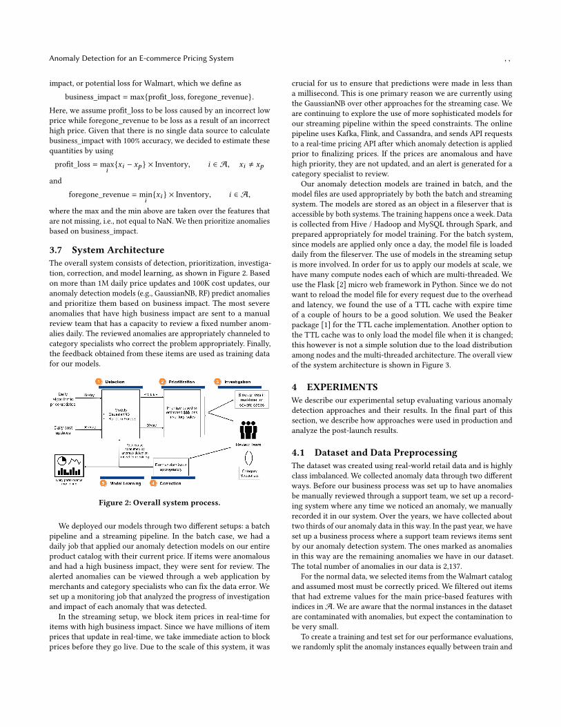
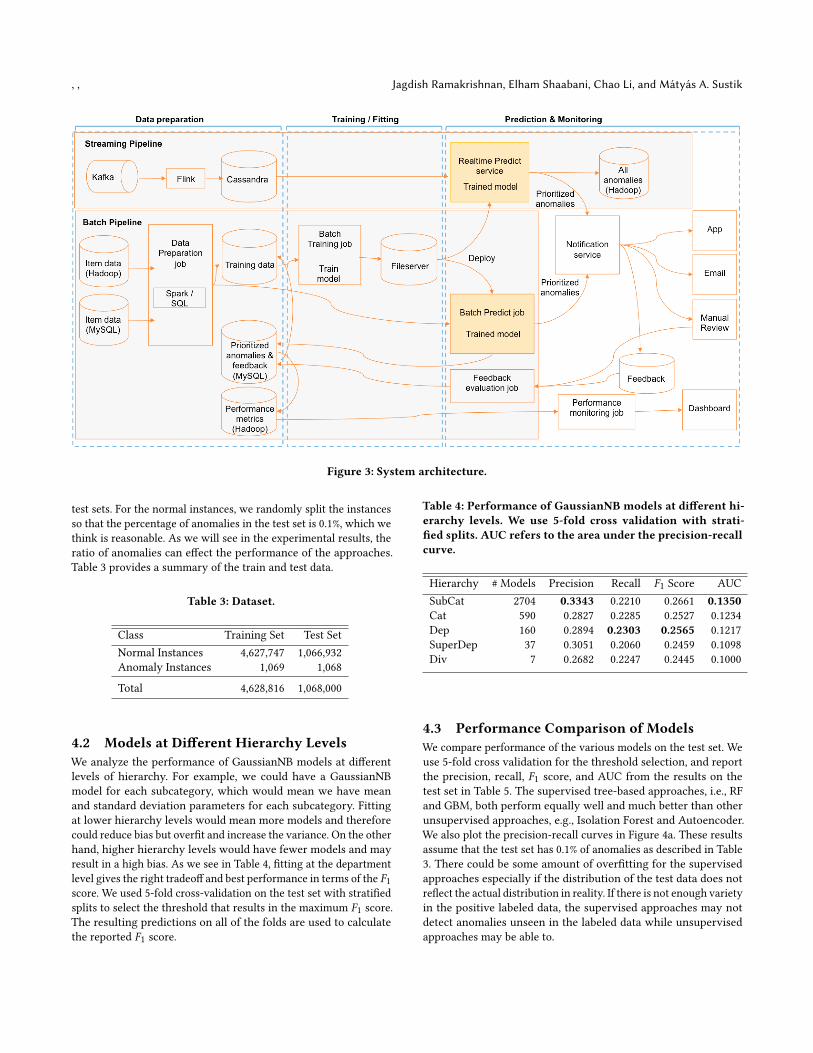
Our anomaly detection models are trained in batch, and themodel files are used appropriately by both the batch and streamingsystem. The models are stored as an object in a fileserver that isaccessible by both systems. The training happens once a week. Datais collected from Hive / Hadoop and MySQL through Spark, andprepared appropriately for model training. For the batch system,since models are applied only once a day, the model file is loadeddaily from the fileserver. The use of models in the streaming setupis more involved. In order for us to apply our models at scale, wehave many compute nodes each of which are multi-threaded. Weuse the Flask [2] micro web framework in Python. Since we do notwant to reload the model file for every request due to the overheadand latency, we found the use of a TTL cache with expire timeof a couple of hours to be a good solution. We used the Beakerpackage [1] for the TTL cache implementation. Another option tothe TTL cache was to only load the model file when it is changed;this however is not a simple solution due to the load distributionamong nodes and the multi-threaded architecture. The overall viewof the system architecture is shown in Figure 3.

4 EXPERIMENTSWe describe our experimental setup evaluating various anomalydetection approaches and their results. In the final part of thissection, we describe how approaches were used in production andanalyze the post-launch results.

4.1 Dataset and Data PreprocessingThe dataset was created using real-world retail data and is highlyclass imbalanced. We collected anomaly data through two differentways. Before our business process was set up to have anomaliesbe manually reviewed through a support team, we set up a record-ing system where any time we noticed an anomaly, we manuallyrecorded it in our system. Over the years, we have collected abouttwo thirds of our anomaly data in this way. In the past year, we haveset up a business process where a support team reviews items sentby our anomaly detection system. The ones marked as anomaliesin this way are the remaining anomalies we have in our dataset.The total number of anomalies in our data is 2,137.

For the normal data, we selected items from the Walmart catalogand assumed most must be correctly priced. We filtered out itemsthat had extreme values for the main price-based features withindices inA. We are aware that the normal instances in the datasetare contaminated with anomalies, but expect the contamination tobe very small.

To create a training and test set for our performance evaluations,we randomly split the anomaly instances equally between train and

, , Jagdish Ramakrishnan, Elham Shaabani, Chao Li, and Mátyás A. Sustik

Figure 3: System architecture.

test sets. For the normal instances, we randomly split the instancesso that the percentage of anomalies in the test set is 0.1%, which wethink is reasonable. As we will see in the experimental results, theratio of anomalies can effect the performance of the approaches.Table 3 provides a summary of the train and test data.

Table 3: Dataset.

Class Training Set Test SetNormal Instances 4,627,747 1,066,932Anomaly Instances 1,069 1,068

Total 4,628,816 1,068,000

4.2 Models at Different Hierarchy LevelsWe analyze the performance of GaussianNB models at differentlevels of hierarchy. For example, we could have a GaussianNBmodel for each subcategory, which would mean we have meanand standard deviation parameters for each subcategory. Fittingat lower hierarchy levels would mean more models and thereforecould reduce bias but overfit and increase the variance. On the otherhand, higher hierarchy levels would have fewer models and mayresult in a high bias. As we see in Table 4, fitting at the departmentlevel gives the right tradeoff and best performance in terms of the F1score. We used 5-fold cross-validation on the test set with stratifiedsplits to select the threshold that results in the maximum F1 score.The resulting predictions on all of the folds are used to calculatethe reported F1 score.

Table 4: Performance of GaussianNB models at different hi-erarchy levels. We use 5-fold cross validation with strati-fied splits. AUC refers to the area under the precision-recallcurve.

Hierarchy # Models Precision Recall F1 Score AUCSubCat 2704 0.3343 0.2210 0.2661 0.1350Cat 590 0.2827 0.2285 0.2527 0.1234Dep 160 0.2894 0.2303 0.2565 0.1217SuperDep 37 0.3051 0.2060 0.2459 0.1098Div 7 0.2682 0.2247 0.2445 0.1000

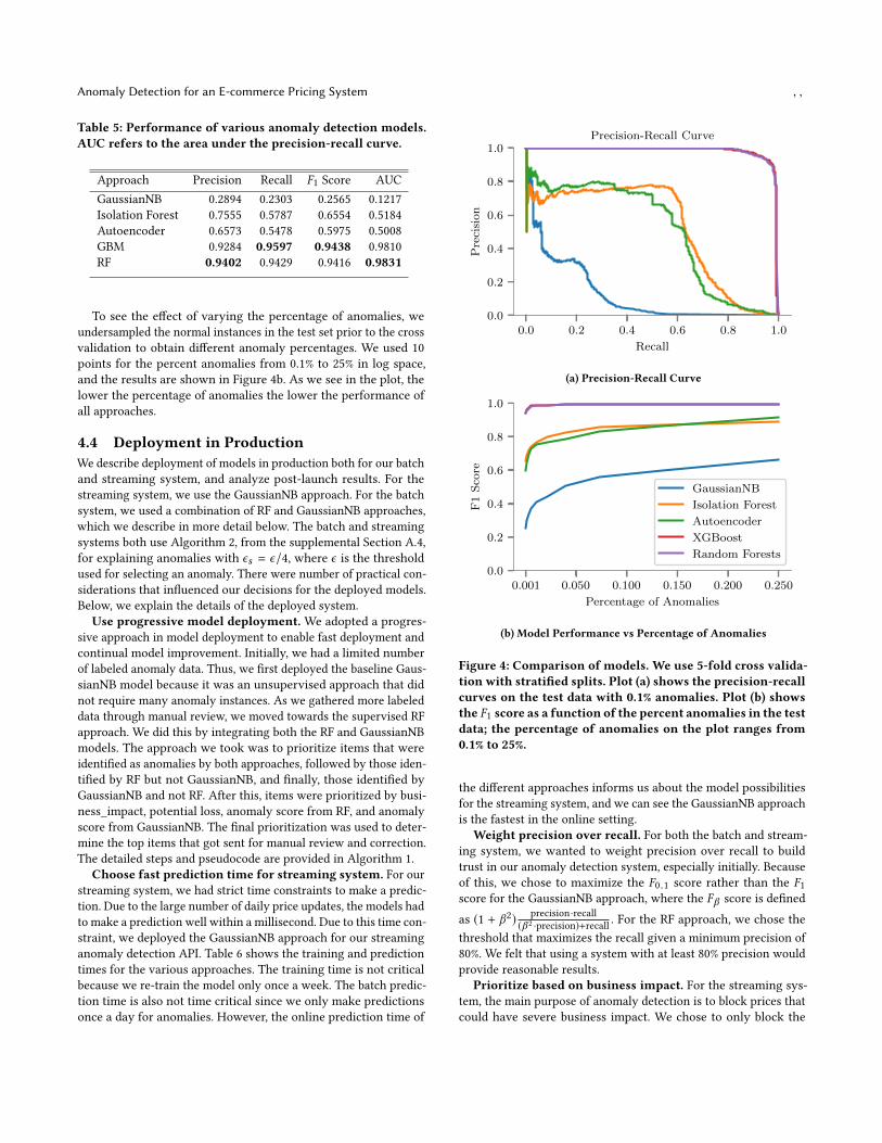
4.3 Performance Comparison of ModelsWe compare performance of the various models on the test set. Weuse 5-fold cross validation for the threshold selection, and reportthe precision, recall, F1 score, and AUC from the results on thetest set in Table 5. The supervised tree-based approaches, i.e., RFand GBM, both perform equally well and much better than otherunsupervised approaches, e.g., Isolation Forest and Autoencoder.We also plot the precision-recall curves in Figure 4a. These resultsassume that the test set has 0.1% of anomalies as described in Table3. There could be some amount of overfitting for the supervisedapproaches especially if the distribution of the test data does notreflect the actual distribution in reality. If there is not enough varietyin the positive labeled data, the supervised approaches may notdetect anomalies unseen in the labeled data while unsupervisedapproaches may be able to.

Anomaly Detection for an E-commerce Pricing System , ,

Table 5: Performance of various anomaly detection models.AUC refers to the area under the precision-recall curve.

Approach Precision Recall F1 Score AUCGaussianNB 0.2894 0.2303 0.2565 0.1217Isolation Forest 0.7555 0.5787 0.6554 0.5184Autoencoder 0.6573 0.5478 0.5975 0.5008GBM 0.9284 0.9597 0.9438 0.9810RF 0.9402 0.9429 0.9416 0.9831

To see the effect of varying the percentage of anomalies, weundersampled the normal instances in the test set prior to the crossvalidation to obtain different anomaly percentages. We used 10points for the percent anomalies from 0.1% to 25% in log space,and the results are shown in Figure 4b. As we see in the plot, thelower the percentage of anomalies the lower the performance ofall approaches.

4.4 Deployment in ProductionWe describe deployment of models in production both for our batchand streaming system, and analyze post-launch results. For thestreaming system, we use the GaussianNB approach. For the batchsystem, we used a combination of RF and GaussianNB approaches,which we describe in more detail below. The batch and streamingsystems both use Algorithm 2, from the supplemental Section A.4,for explaining anomalies with ϵs = ϵ/4, where ϵ is the thresholdused for selecting an anomaly. There were number of practical con-siderations that influenced our decisions for the deployed models.Below, we explain the details of the deployed system.

Use progressive model deployment. We adopted a progres-sive approach in model deployment to enable fast deployment andcontinual model improvement. Initially, we had a limited numberof labeled anomaly data. Thus, we first deployed the baseline Gaus-sianNB model because it was an unsupervised approach that didnot require many anomaly instances. As we gathered more labeleddata through manual review, we moved towards the supervised RFapproach. We did this by integrating both the RF and GaussianNBmodels. The approach we took was to prioritize items that wereidentified as anomalies by both approaches, followed by those iden-tified by RF but not GaussianNB, and finally, those identified byGaussianNB and not RF. After this, items were prioritized by busi-ness_impact, potential loss, anomaly score from RF, and anomalyscore from GaussianNB. The final prioritization was used to deter-mine the top items that got sent for manual review and correction.The detailed steps and pseudocode are provided in Algorithm 1.

Choose fast prediction time for streaming system. For ourstreaming system, we had strict time constraints to make a predic-tion. Due to the large number of daily price updates, the models hadto make a prediction well within a millisecond. Due to this time con-straint, we deployed the GaussianNB approach for our streaminganomaly detection API. Table 6 shows the training and predictiontimes for the various approaches. The training time is not criticalbecause we re-train the model only once a week. The batch predic-tion time is also not time critical since we only make predictionsonce a day for anomalies. However, the online prediction time of

0.0 0.2 0.4 0.6 0.8 1.0

Recall

0.0

0.2

0.4

0.6

0.8

1.0

Pre

cisi

on

Precision-Recall Curve

(a) Precision-Recall Curve

0.001 0.050 0.100 0.150 0.200 0.250

Percentage of Anomalies

0.0

0.2

0.4

0.6

0.8

1.0

F1

Sco

reGaussianNB

Isolation Forest

Autoencoder

XGBoost

Random Forests

(b) Model Performance vs Percentage of Anomalies

Figure 4: Comparison of models. We use 5-fold cross valida-tion with stratified splits. Plot (a) shows the precision-recallcurves on the test data with 0.1% anomalies. Plot (b) showsthe F1 score as a function of the percent anomalies in the testdata; the percentage of anomalies on the plot ranges from0.1% to 25%.

the different approaches informs us about the model possibilitiesfor the streaming system, and we can see the GaussianNB approachis the fastest in the online setting.

Weight precision over recall. For both the batch and stream-ing system, we wanted to weight precision over recall to buildtrust in our anomaly detection system, especially initially. Becauseof this, we chose to maximize the F0.1 score rather than the F1score for the GaussianNB approach, where the Fβ score is definedas (1 + β2) precision·recall

(β 2 ·precision)+recall . For the RF approach, we chose thethreshold that maximizes the recall given a minimum precision of80%. We felt that using a system with at least 80% precision wouldprovide reasonable results.

Prioritize based on business impact. For the streaming sys-tem, the main purpose of anomaly detection is to block prices thatcould have severe business impact. We chose to only block the

, , Jagdish Ramakrishnan, Elham Shaabani, Chao Li, and Mátyás A. Sustik

Algorithm 1: Combined GaussianNB and Random Forest pre-dictions that was used in production.1 function combined_predict (X,L);Input :matrix X containing features for samples, list L with

issue names for getting suspected issuesOutput :vectors is_anomaly, priority, suspected_issues

2 is_anomaly_G, score_G = GaussianNB.predict(X)3 is_anomaly_RF, score_RF = RandomForest.predict(X)4 is_anomaly = is_anomaly_G OR is_anomaly_RF5 suspected_issues = get_suspected_issues(X,L)6 priority, business_impact = business_prioritization(X)7 Sort descending by is_anomaly_RF, is_anomaly_G, priority,

business_impact, score_G, and score_RF.8 return is_anomaly, priority, suspected_issues

Table 6: Training and prediction times of anomaly detectionmodels. We randomly sampled 1000 items from the test setwith 25% anomalies and reported the time from predictingthem all at once (batch) and one-by-one (online). The predic-tion times are the average prediction time per item both forbatch and online.

Approach Train Batch Onlinetime [s] Prediction Prediction

time [ms] time [ms]GaussianNB 451.487 0.021 0.091Isolation Forest 396.229 0.078 29.902Autoencoder 6853.187 0.026 0.934GBM 3138.834 0.005 0.169RF 3794.588 0.321 215.925

prices that had the highest priority according to our prioritizationlogic. Once a price is blocked a category specialist is alerted throughour web application, where they take actions to correct the issueor override with a manual price. For the batch system, we had afixed capacity of alerts that could be reviewed by support team ona daily basis.

Results from production launch. For the streaming system,while we have data on created alerts, the alerts were not thoroughlyreviewed; the prices were automatically blocked due to the severityand only some alerts resulted in price corrections. In the batchsystem, however, every alert was reviewed through a support teamand resolved as either a false positive or true positive and correctedappropriately. We analyzed the post-launch data for the batch sys-tem that we deployed. The approach used was the combined RFand GaussianNB approaches that we described earlier.

A total of 5,205 alerts were generated over two months, andonly 1,625 alerts had a resolution. The typical total review time canvaried between a week to a couple of weeks. Alerts were reviewedby a support team and appropriately directed to a team or a categoryspecialist who is an expert on the specific item referenced. Oncea category specialist determines whether there is an issue, theycorrect it if needed, and then, the alert is marked with a resolution.

As shown in Table 7, there were 836 false positive, resulting ina precision of 53.5% among the alerts generated. It is not possibleto measure recall because we do not actually know about existinganomalies. The actual precision of 53.5% is significantly below thedesired 80% precision. In order to understand further if there wasa bug or a systematic problem with our deployed approach, weconducted error analysis on on 100 randomly sampled alerts out ofthe 756 that were marked false positives. Our second review foundthat about 49% of the items that were marked false positives wereactually not false positives, and there was a systematic issue withthe labeling. From category specialist point of view, if an item has acorrect price and cost, everything is fine. However, for many items,even with a correct price and cost, there may be issues with otheritem data that could impact prices in the future. Indeed, our reviewteam was marking items detected by our system with incorrectcompetitor prices as false positives. We believe these are not falsepositives, and our models were designed to catch these types ofissues. If we adjust for this systematic error by generalizing the49% error rate over the fully reviewed set, this could change theprecision from 53.5% to 76.2%, bringing it much closer to the 80%desired precision. The original and adjusted numbers are reportedin Table 7. Besides addressing this competitor price issue, we areworking on ways to improve our manual review process, e.g., havemultiple reviews for a subset of items for quality assurance.

Table 7: Results from production launch. FP refers to thenumber of False Positives, i.e., number of predictions thatwere not actually anomalies.

# Alerts # Reviewed # FP PrecisionOriginal 5,205 1,625 756 53.5%Adjusted 5,205 1,625 386 76.2%

5 CONCLUSIONWe proposed an anomaly detection framework forWalmart’s onlinepricing system. Our models were able to detect the most importantanomalies effectively by finding mis-priced items and incorrectdata inputs to our pricing algorithm. Besides detecting anomalies,we developed an approach that relies on the anomaly scores froma density model to explain the anomalies detected. In order toconcentrate on the most important anomalies to review and inturn further gather labeled data for our models, we used estimatedbusiness impact and other pertinent item information to prioritizethe anomalies. We trained and evaluated various unsupervised andsupervised approaches using real-world retail data. After selectingthe appropriate models, we successfully deployed our approachesin production and achieved the desired precision of detection.

For future work, we can explore methods that systematically in-corporate overlapping hierarchy levels such as done in [12] througha maximum entropy formulation; in this paper, we consideredhierarchical-based features by either using them as label encodedor as a one-hot vector. We can further consider more sophisticatedlearning-based models for explaining anomalies, such as [33]. An-other idea is to explore more extensive time series features suchas the ones provided in [15]. Collection of reliable labeled data

Anomaly Detection for an E-commerce Pricing System , ,

is an on-going challenge. Due to the complex nature of anomalydetection, human review is not foolproof. In addition to anomalyreview by a dedicated team, we plan to explore other options suchas crowd sourcing, to improve the accuracy of our data labelingprocess.

6 ACKNOWLEDGEMENTSWe would like to thank the entire Walmart Smart Pricing team fortheir contributions to this project. We thank Marcus Csaky, VarunBahl, Brian Seaman, and Zach Dennett for being very supportiveof this project and for providing feedback on the paper. We thankTracy Phung for her suggestions and work on training data andalerts generation. We thank Ravi Ganti for helpful discussions andsuggestions about the autoencoder model. We thank Andrew Tor-son, Abhiraj Butala, and Vikrant Goel for suggesting the use of aTTL cache for the streaming pipeline. We thank Victor Oleinikovand Paulo Tarasiuk for work on alerting anomalies through a webapplication, Kevin Shah for his work on reviewer feedback, andVaishnavi Ravisankar for her work on performance monitoring.

REFERENCES[1] [n.d.]. Beaker python package. https://beaker.readthedocs.io/en/latest/[2] [n.d.]. Flask python package. http://flask.pocoo.org/docs/0.12/[3] 2015. AnomalyDetection R package. https://github.com/twitter/

AnomalyDetection.[4] 2015. luminol. https://github.com/linkedin/luminol.[5] Charu C. Aggarwal. 2016. Outlier Analysis (2nd ed.). Springer Publishing Com-

pany, Incorporated.[6] Subutai Ahmad and Scott Purdy. 2016. Real-Time Anomaly Detection for Stream-

ing Analytics. CoRR abs/1607.02480 (2016).[7] Fabrizio Angiulli and Clara Pizzuti. 2002. Fast Outlier Detection in High Dimen-

sional Spaces. In Proceedings of the 6th European Conference on Principles of DataMining and Knowledge Discovery (PKDD ’02). Springer-Verlag, London, UK, UK,15–26. http://dl.acm.org/citation.cfm?id=645806.670167

[8] Anodot. [n.d.]. Nipping it in the Bud: How real-time anomaly detection canprevent e-commerce glitches from becoming disasters. https://www.anodot.com/blog/real-time-anomaly-detection-can-prevent-ecommerce-retail-glitches/.

[9] Leo Breiman. 2001. Random Forests. Mach. Learn. 45, 1 (Oct. 2001), 5–32. https://doi.org/10.1023/A:1010933404324

[10] Markus M. Breunig, Hans-Peter Kriegel, Raymond T. Ng, and Jörg Sander. 2000.LOF: Identifying Density-based Local Outliers. SIGMOD Rec. 29, 2 (May 2000),93–104. https://doi.org/10.1145/335191.335388

[11] Tianqi Chen and Carlos Guestrin. 2016. XGBoost: A Scalable Tree BoostingSystem. In Proceedings of the 22Nd ACM SIGKDD International Conference onKnowledge Discovery and Data Mining (KDD ’16). ACM, New York, NY, USA,785–794. https://doi.org/10.1145/2939672.2939785

[12] Miroslav Dudik, David M. Blei, and Robert E. Schapire. 2007. Hierarchical Maxi-mum Entropy Density Estimation. In Proceedings of the 24th International Con-ference on Machine Learning (ICML ’07). ACM, New York, NY, USA, 249–256.https://doi.org/10.1145/1273496.1273528

[13] Jerome H. Friedman. 2001. Greedy function approximation: A gradient boostingmachine. Ann. Statist. 29, 5 (10 2001), 1189–1232. https://doi.org/10.1214/aos/1013203451

[14] Huiyuan Fu, Huadong Ma, and Anlong Ming. 2011. EGMM: An enhanced Gauss-ian mixture model for detecting moving objects with intermittent stops. Pro-ceedings - IEEE International Conference on Multimedia and Expo, 1–6. https://doi.org/10.1109/ICME.2011.6012011

[15] Ben D. Fulcher and Nick S. Jones. 2014. Highly Comparative Feature-BasedTime-Series Classification. IEEE Transactions on Knowledge and Data Engineering26 (2014), 3026–3037.

[16] Nico Görnitz, Marius Kloft, Konrad Rieck, and Ulf Brefeld. 2013. TowardSupervised Anomaly Detection. J. Artif. Int. Res. 46, 1 (Jan. 2013), 235–262.http://dl.acm.org/citation.cfm?id=2512538.2512545

[17] Malay Haldar, Mustafa Abdool, Prashant Ramanathan, Tao Xu, Shulin Yang,Huizhong Duan, Qing Zhang, Nick Barrow-Williams, Bradley C. Turnbull, Bren-dan M. Collins, and Thomas Legrand. 2018. Applying Deep Learning To AirbnbSearch. CoRR abs/1810.09591 (2018). arXiv:1810.09591 http://arxiv.org/abs/1810.09591

[18] R. J. Hyndman, E. Wang, and N. Laptev. 2015. Large-Scale Unusual Time Se-ries Detection. In 2015 IEEE International Conference on Data Mining Workshop

(ICDMW). 1616–1619. https://doi.org/10.1109/ICDMW.2015.104[19] Sevvandi Kandanaarachchi, Mario A Munoz, Rob J Hyndman, and Kate Smith-

Miles. 2018. On normalization and algorithm selection for unsupervised outlierdetection. Monash Econometrics and Business Statistics Working Papers 16/18.Monash University, Department of Econometrics and Business Statistics. https://ideas.repec.org/p/msh/ebswps/2018-16.html

[20] JooSeuk Kim and Clayton D. Scott. 2011. Robust Kernel Density Estimation.Acoustics, Speech, and Signal Processing, 1988. ICASSP-88., 1988 International Con-ference on 13 (07 2011).

[21] Diederik Kingma and Jimmy Ba. 2014. Adam: A Method for Stochastic Optimiza-tion. International Conference on Learning Representations (12 2014).

[22] Hans-Peter Kriegel, Matthias Schubert, and Arthur Zimek. 2008. Angle-basedOutlier Detection in High-dimensional Data. In Proceedings of the 14th ACMSIGKDD International Conference on Knowledge Discovery and Data Mining (KDD’08). ACM, New York, NY, USA, 444–452. https://doi.org/10.1145/1401890.1401946

[23] Nikolay Laptev. 2018. AnoGen: Deep Anomaly Generator. TechnicalReport. Facebook. https://research.fb.com/wp-content/uploads/2018/11/AnoGen-Deep-Anomaly-Generator.pdf?

[24] Nikolay Laptev, Saeed Amizadeh, and Ian Flint. 2015. Generic and ScalableFramework for Automated Time-series Anomaly Detection. In Proceedings of the21th ACM SIGKDD International Conference on Knowledge Discovery and DataMining (KDD ’15). ACM, New York, NY, USA, 1939–1947. https://doi.org/10.1145/2783258.2788611

[25] Fei Tony Liu, Kai Ming Ting, and Zhi-Hua Zhou. 2008. Isolation Forest. InProceedings of the 2008 Eighth IEEE International Conference on Data Mining(ICDM ’08). IEEE Computer Society, Washington, DC, USA, 413–422. https://doi.org/10.1109/ICDM.2008.17

[26] Travis Oliphant. 2006–. NumPy: A guide to NumPy. USA: Trelgol Publishing.http://www.numpy.org/ [Online; accessed <today>].

[27] F. Pedregosa, G. Varoquaux, A. Gramfort, V. Michel, B. Thirion, O. Grisel, M.Blondel, P. Prettenhofer, R. Weiss, V. Dubourg, J. Vanderplas, A. Passos, D. Cour-napeau, M. Brucher, M. Perrot, and E. Duchesnay. 2011. Scikit-learn: MachineLearning in Python. Journal of Machine Learning Research 12 (2011), 2825–2830.

[28] Tomáš Pevn? 2016. Loda: Lightweight On-line Detector of Anomalies. Mach.Learn. 102, 2 (Feb. 2016), 275–304. https://doi.org/10.1007/s10994-015-5521-0

[29] Maheshkumar R Sabhnani, Daniel B Neill, and AndrewWMoore. 2005. Detectinganomalous patterns in pharmacy retail data. (01 2005).

[30] Bernhard Schölkopf, John C. Platt, John Shawe-Taylor, Alexander J. Smola, andRobert C. Williamson. 2001. Estimating the Support of a High-DimensionalDistribution. Neural Computation 13 (2001), 1443–1471.

[31] Bernhard Schölkopf, Robert Williamson, Alex Smola, John Shawe-Taylor, andJohn Platt. 1999. Support Vector Method for Novelty Detection. In Proceedingsof the 12th International Conference on Neural Information Processing Systems(NIPS’99). MIT Press, Cambridge, MA, USA, 582–588. http://dl.acm.org/citation.cfm?id=3009657.3009740

[32] Dominique Shipmon, Jason Gurevitch, Paolo M Piselli, and Steve Edwards. 2017.Time Series Anomaly Detection: Detection of Anomalous Drops with Limited Featuresand Sparse Examples in Noisy Periodic Data. Technical Report. Google Inc. https://arxiv.org/abs/1708.03665

[33] Md Amran Siddiqui, Alan Fern, Thomas G. Dietterich, and Weng-Keen Wong.2019. Sequential Feature Explanations for Anomaly Detection. ACM Trans. Knowl.Discov. Data 13, 1, Article 1 (Jan. 2019), 22 pages. https://doi.org/10.1145/3230666

[34] Karanjit Singh and Shuchita Upadhyaya. 2012. Outlier Detection: ApplicationsAnd Techniques. International Journal of Computer Science Issues 9 (01 2012).

[35] David M.J. Tax and Robert P.W. Duin. 2004. Support Vector Data Description.Machine Learning 54, 1 (01 Jan 2004), 45–66. https://doi.org/10.1023/B:MACH.0000008084.60811.49

[36] Owen Vallis, Jordan Hochenbaum, and Arun Kejariwal. 2014. A Novel Techniquefor Long-Term Anomaly Detection in the Cloud. In 6th USENIX Workshop onHot Topics in Cloud Computing (HotCloud 14). USENIX Association, Philadel-phia, PA. https://www.usenix.org/conference/hotcloud14/workshop-program/presentation/vallis

[37] Houssam Zenati, Chuan Sheng Foo, Bruno Lecouat, Gaurav Manek, and Vijay Ra-maseshan Chandrasekhar. 2018. Efficient GAN-Based Anomaly Detection. CoRRabs/1802.06222 (2018). arXiv:1802.06222 http://arxiv.org/abs/1802.06222

[38] Shuangfei Zhai, Yu Cheng, Weining Lu, and Zhongfei Zhang. 2016. Deep Struc-tured Energy Based Models for Anomaly Detection. In Proceedings of the 33rdInternational Conference on International Conference onMachine Learning - Volume48 (ICML’16). JMLR.org, 1100–1109. http://dl.acm.org/citation.cfm?id=3045390.3045507

[39] Yue Zhao, Zain Nasrullah, and Zheng Li. 2019. PyOD: A Python Toolbox forScalable Outlier Detection. arXiv preprint arXiv:1901.01588 (2019). https://arxiv.org/abs/1901.01588

[40] Lingxue Zhu and Nikolay Laptev. 2017. Deep and Confident Prediction for TimeSeries at Uber. 103–110. https://doi.org/10.1109/ICDMW.2017.19

, , Jagdish Ramakrishnan, Elham Shaabani, Chao Li, and Mátyás A. Sustik

A SUPPLEMENTARY INFORMATIONImplementation of approaches can be obtained athttps://github.com/walmartlabs/anomaly-detection-walmart.

A.1 Python PackagesWe used the pyod python package [39] for the Autoencoder ap-proach. For the Isolation forest, RF, and GBM implementations, weused the scikit-learn package [27]. For GBM, we use the scikit-learnAPI for XGBoost [11]. For the GaussianNB approach, we wrotecustom code using the numpy package [26].

A.2 Experiment DetailsFor the GaussianNB approach, we fit models on the departmentlevel, which meant we had a separate GaussianNB model for eachdepartment. There were 160 departments in our training and testdata and therefore models. For some predictions, an item had anew department label that was unseen in the training data; forthese cases, we used a GaussianNB model that was trained on theentire training data with data from all departments. We ensuredthat every model had at least 9 samples for fitting; if not, we fit themodel at one level higher in the hierarchy, i.e., super-department.We ensured a minimum standard deviation of 0.01 by clipping it ifit went below 0.01.

For Isolation Forest, we used 100 estimators, 5% of the trainingset as the number of samples, and 10% of the features to traineach base estimator. Initially, we used a fixed number of samplesto train estimators, e.g., 512, but we found that the performancewas severely impacted due to the low number of samples; 5% ofthe training set (roughly 200K samples) worked well for us. Forthe Autoencoder model, we used 64, 32, 32, and 64 units for theencoder and decoder hidden layers respectively. We used ReLUactivations for all hidden layers and a tanh activation for the outputlayer. We standardized the data prior to feeding to the input layer.We used mean squared error as the loss, i.e., the anomaly score,512 for the batch size, 100 epochs to train the network, and theAdam optimizer [21]. We used a 0.2 dropout rate, and 0.1 for theregularization strength of a activity_regularizer on every layer.Most of these choices were defaults from the pyod package [39].We used 100 estimators and a max depth of 5 for GBM, and we used400 estimators and a max depth of 80 for RF.

A.3 Computing ResourcesFor all comparisons of the approaches, we requested the same cloudcomputing resources for fitting and prediction. We used a singlenode with 5 CPU cores and 45GB of RAM.

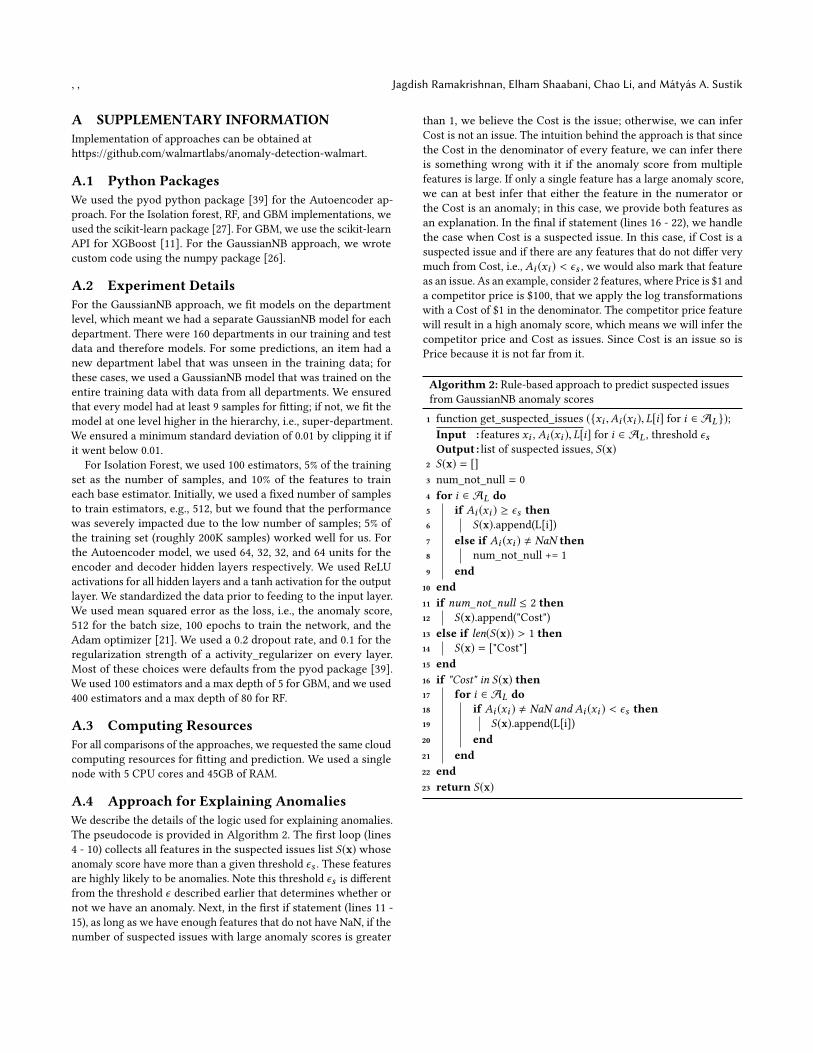
A.4 Approach for Explaining AnomaliesWe describe the details of the logic used for explaining anomalies.The pseudocode is provided in Algorithm 2. The first loop (lines4 - 10) collects all features in the suspected issues list S(x) whoseanomaly score have more than a given threshold ϵs . These featuresare highly likely to be anomalies. Note this threshold ϵs is differentfrom the threshold ϵ described earlier that determines whether ornot we have an anomaly. Next, in the first if statement (lines 11 -15), as long as we have enough features that do not have NaN, if thenumber of suspected issues with large anomaly scores is greater

than 1, we believe the Cost is the issue; otherwise, we can inferCost is not an issue. The intuition behind the approach is that sincethe Cost in the denominator of every feature, we can infer thereis something wrong with it if the anomaly score from multiplefeatures is large. If only a single feature has a large anomaly score,we can at best infer that either the feature in the numerator orthe Cost is an anomaly; in this case, we provide both features asan explanation. In the final if statement (lines 16 - 22), we handlethe case when Cost is a suspected issue. In this case, if Cost is asuspected issue and if there are any features that do not differ verymuch from Cost, i.e., Ai (xi ) < ϵs , we would also mark that featureas an issue. As an example, consider 2 features, where Price is $1 anda competitor price is $100, that we apply the log transformationswith a Cost of $1 in the denominator. The competitor price featurewill result in a high anomaly score, which means we will infer thecompetitor price and Cost as issues. Since Cost is an issue so isPrice because it is not far from it.

Algorithm 2: Rule-based approach to predict suspected issuesfrom GaussianNB anomaly scores1 function get_suspected_issues ({xi ,Ai (xi ),L[i] for i ∈ AL});Input : features xi , Ai (xi ),L[i] for i ∈ AL , threshold ϵsOutput : list of suspected issues, S(x)

2 S(x) = []3 num_not_null = 04 for i ∈ AL do5 if Ai (xi ) ≥ ϵs then6 S(x).append(L[i])7 else if Ai (xi ) , NaN then8 num_not_null += 19 end

10 end11 if num_not_null ≤ 2 then12 S(x).append("Cost")13 else if len(S(x)) > 1 then14 S(x) = ["Cost"]15 end16 if "Cost" in S(x) then17 for i ∈ AL do18 if Ai (xi ) , NaN and Ai (xi ) < ϵs then19 S(x).append(L[i])20 end21 end22 end23 return S(x)