Annular Modes and their Climate Impactsin the GFDL Coupled Ocean-Atmosphere Model

Alex Hall and Martin VisbeckLamont-Doherty Earth Observatory

of Columbia UniversityPO Box 1000, 61 Route 9W

Palisades, NY 10964-8000

contact information:Alex Hall

Tel: (914) 365-8875

FAX: (914) 365-8736e-mail: alexhall@rosie.ldeo.columbia.edu

submitted to Journal of Climate

Abstract

In the first part of this paper, we characterize the wintertime ‘annular modes’

in an 800 year integration of the GFDL R15 coupled ocean-atmosphere model.

In both hemispheres, the first EOF of surface pressure is almost perfectly de-

scribed as an oscillation of mass between mid and high latitudes. However,

in the northern hemisphere (NH), the mid-latitude mass distribution associated

with the annular mode is concentrated in lobes over the North Atlantic and Pa-

cific, while in the southern hemisphere (SH), the distribution is nearly zonally

symmetric. In the NH, the annular mode is also biased toward the Atlantic

sector, with the most coherent out-of-phase pressure relationship occurring be-

tween Iceland and the Azores, while in the SH, the bias toward any particular

longitude is weaker. The SH annular mode is therefore more ‘annular’ than its

NH counterpart. In these respects the simulated annular modes are similar to

the observed annular modes, except that the Pacific lobe of the simulated NH

mode is too intense. The spectra of the NH and SH annular modes indices are

white. They also show that both NH and SH annular modes have approximately

the same total variance.

In the second part, we examine the simulated climate impacts of the SH

annular mode. Compared to the NH, the surface air temperature anomalies as-

sociated with the SH annular mode are small. However, the strong geostrophic

winds implied by the circular pole-centered pressure pattern of the annular mode

have significant implications for the ocean. When the annular mode is in a pos-

itive phase (analogous arguments apply for the negative phase), these winds

induce a northward Ekman current in the upper layer of the circumpolar ocean.

This Ekman pumping explains most of the variability of the circumpolar current’s

meridional component. Through mass conservation, this circulation leads to up-

welling near the edge of the Antarctica, and downwelling just north of the circum-

polar current, accounting for much of the upwelling variability in this region. By

altering the meridional temperature gradient, these upwelling and downwelling

anomalies lead to variations in the intensity of the circumpolar current; for time

scales shorter than 50 years, the correlation between the SH annular mode

index and the total transport across the Drake Passage is 0.8. Finally, the Ek-

man pumping advects sea ice away from Antarctica, resulting in thinner sea ice

around the continent, and thicker ice closer to the ice margin. Because the ice

thickness pattern associated with the annular mode is so ring-like, the annular

1

mode accounts for most of the variability in total areal coverage of sea ice; for

time scales longer than 10 years, the correlation between the SH annular mode

index and ice coverage is 0.6.

1 Introduction

Enough measurements exist to characterize the dominant mode of variability pole-ward of 20� in both the northern and southern hemispheres (NH and SH): it can be

roughly described as an oscillation of mass between mid and high latitudes. Theteleconnection between mid and high latitude pressure was first recognized in theNorth Atlantic sector of the NH, where measurements are relatively plentiful. Walker

and Bliss (1924), analyzing North Atlantic temperature and pressure data, coinedthe term ‘North Atlantic Oscillation’ (NAO) to describe the out-of-phase relationship

between pressure over the Azores and Iceland. Armed with better observations,Kutzbach (1970) and Wallace and Gutzler (1981) also examined and quantified this

teleconnection. One theme of all these studies is that the dominant mode of variabil-ity is best identified by the most prominent teleconnection (i.e. the two points where

the pressure anti-correlation is largest). These two points lie in the Atlantic sector.More recently, empirical orthogonal function (EOF) analysis has become a basis

for identifying modes of variability. This technique, which identifies the mode thataccounts for the most overall variability, is highlighted in papers by Thompson andWallace (Thompson and Wallace 1998 and Thompson and Wallace 1999). They

found that the first EOF of the pressure field has a ring-like structure, with pressurein both the Atlantic and Pacific sectors out-of-phase with pressure over the Arctic. In

addition, they analyzed SH data, and showed that an analogous, nearly zonally sym-metric pressure oscillation between mid and high latitudes exists there. Because this

ring-like structure is present in both hemispheres, they proposed the term ‘annularmode’ to describe the dominant mode of variability in mid to high latitudes. We will

rely on this definition throughout this paper.In this study, we analyze the behavior of annular modes in a long-term inte-

gration of the GFDL coarse resolution coupled ocean-atmosphere model (describedin section 2). One of our aims is to explore how physical understanding of the dom-

inant mode of simulated variability in both hemispheres is influenced by analysis

2

technique. Thus we will compare results based on the most prominent surface pres-sure teleconnection to results based on EOF analysis of the surface pressure field.

To test the limits of the annular mode concept, we also wish to examine the picturethat emerges by assuming that the dominant mode of variability is perfectly annular.

Thus we will use the zonal-mean pressure difference between mid and high latitudesto define an index of annular mode variability. In total, we will have three methods

to examine the annular modes. It turns out that physical understanding is enhancedby examining results from all three techniques together, allowing us to arrive at aunified picture of the annular modes, including a comparison of the modes’ behavior

in the northern and southern hemispheres. This portion of our study is presentedin section 3. Then, in section 4, we examine the simulated climate impacts of the

annular modes. Since this issue is relatively well-understood for the dominant modeof variability in the NH, we will focus on the climate impacts of the SH annular mode.

Relatively little has been written about the behavior of annular modes in mod-els. This is unfortunate, since a physically-based numerical model of the climate can

complement understanding based on observations nicely. First, it can provide longtime series that are much more stable and reliable in a statistical sense than ob-

servational time series. Second, it provides global data coverage. To study theSH annular mode, this is especially useful because of sparsity of measurements

in the SH poleward of 30�S. The fact that we are using a model that includes anoceanic component is also helpful; as we will show, the SH annular mode has in-teresting and potentially significant oceanographic implications. At the present time,

adequate ocean observations are not readily available to address this issue.

2 Model Description

The most important features of this model are described in some detail in Manabe etal. (1991). It consists of a general circulation model of the ocean coupled to an atmo-

spheric general circulation model through exchange of heat, water, and momentum.The variables of the nine-vertical-level atmospheric component are represented in

the horizontal by a series of spherical harmonics (rhomboidal truncation at zonalwavenumber 15) and corresponding grid point values (7.5� longitude by about 4.5�

latitude gridbox size). The radiative transfer calculation includes a seasonal cycle

3

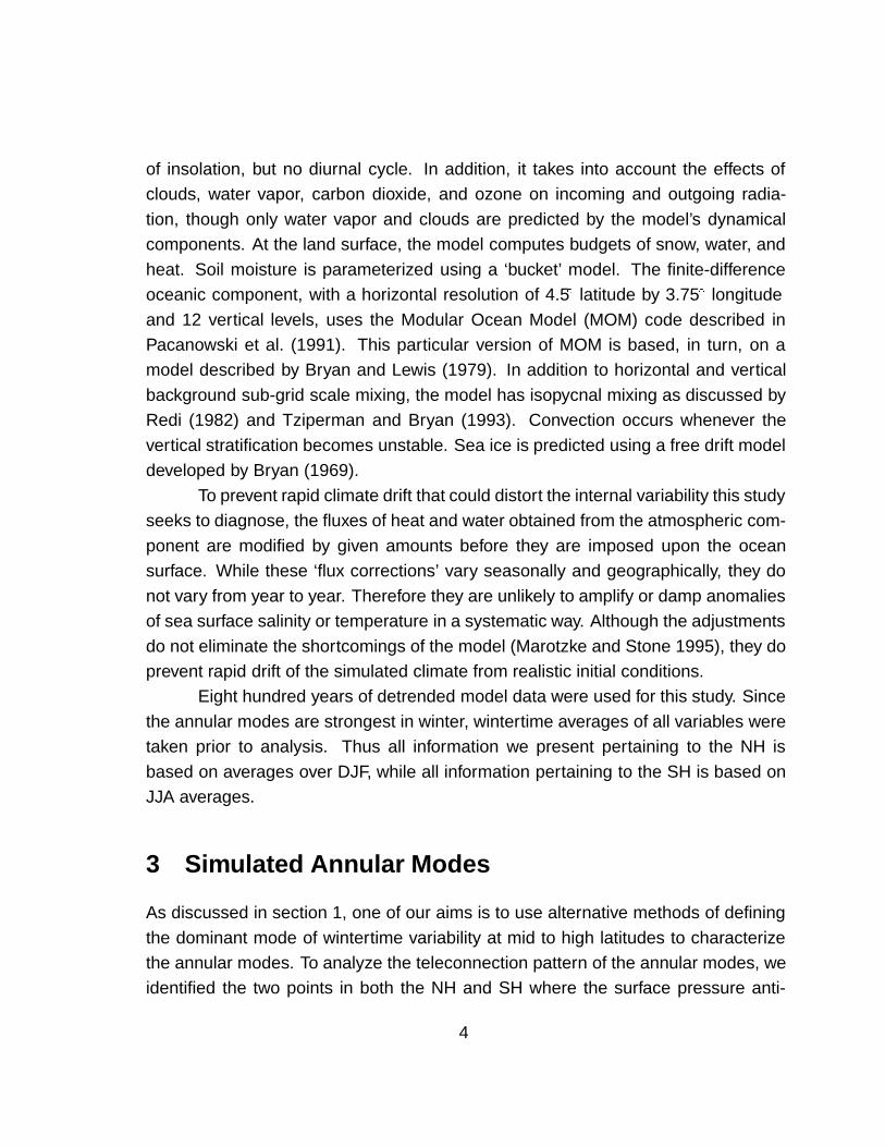
of insolation, but no diurnal cycle. In addition, it takes into account the effects ofclouds, water vapor, carbon dioxide, and ozone on incoming and outgoing radia-

tion, though only water vapor and clouds are predicted by the model’s dynamicalcomponents. At the land surface, the model computes budgets of snow, water, and

heat. Soil moisture is parameterized using a ‘bucket’ model. The finite-differenceoceanic component, with a horizontal resolution of 4.5� latitude by 3.75� longitude

and 12 vertical levels, uses the Modular Ocean Model (MOM) code described inPacanowski et al. (1991). This particular version of MOM is based, in turn, on amodel described by Bryan and Lewis (1979). In addition to horizontal and vertical

background sub-grid scale mixing, the model has isopycnal mixing as discussed byRedi (1982) and Tziperman and Bryan (1993). Convection occurs whenever the

vertical stratification becomes unstable. Sea ice is predicted using a free drift modeldeveloped by Bryan (1969).

To prevent rapid climate drift that could distort the internal variability this studyseeks to diagnose, the fluxes of heat and water obtained from the atmospheric com-

ponent are modified by given amounts before they are imposed upon the oceansurface. While these ‘flux corrections’ vary seasonally and geographically, they do

not vary from year to year. Therefore they are unlikely to amplify or damp anomaliesof sea surface salinity or temperature in a systematic way. Although the adjustments

do not eliminate the shortcomings of the model (Marotzke and Stone 1995), they doprevent rapid drift of the simulated climate from realistic initial conditions.

Eight hundred years of detrended model data were used for this study. Since

the annular modes are strongest in winter, wintertime averages of all variables weretaken prior to analysis. Thus all information we present pertaining to the NH is

based on averages over DJF, while all information pertaining to the SH is based onJJA averages.

3 Simulated Annular Modes

As discussed in section 1, one of our aims is to use alternative methods of defining

the dominant mode of wintertime variability at mid to high latitudes to characterizethe annular modes. To analyze the teleconnection pattern of the annular modes, weidentified the two points in both the NH and SH where the surface pressure anti-

4

2

1

0

0−1−2−3

−4

−5

−6

123

−3

1 0

1

−2

−1

0

1

−1

32

1

0

12

0 −1

−2−3

−4−4−5

−3

1 10−1

−2−3

1

02

1

0−1

−2−3

−3−3

2

1

0

−1−5−5

−4

−3−2−1

01

2

0

MAC ZPD EOF

Figure 1: The pressure patterns associated with the MAC, ZPD, and EOF indices.

Units are hPa. Model geography is suppressed to facilitate orientation.

correlation is largest. These points are centered on 70�N, 26�W and 38�N, 34�Win the NH, and 70�S, 56�E and 38�S, 101�E in the SH. Note that the latitudes ofthese points are the same in both hemispheres. An index was then defined as the

surface pressure difference between the low and high latitude points. This index willbe identified throughout this paper as the Maximum Anti-Correlation (MAC) index.

To create the index measuring the zonally symmetric aspect of the annular modes,we calculated the zonal-mean surface pressure difference at the latitudes where

the points defining the MAC index are located (70� and 38�). This index is will beidentified as the Zonal-mean Pressure Difference (ZPD) index. Finally, the index that

captures the most pressure variability was defined as the time series associated withthe first EOF of wintertime surface pressure (EOF index). Pressure data over the

entire hemisphere was used to calculate the EOF.Figure 1 shows the pressure patterns associated with the MAC, ZPD and

5

EOF indices. In the case of the MAC and ZPD indices, these patterns are givenby the regression of local surface pressure onto the indices. Before the regressions

were calculated, the MAC and ZPD time series were normalized so that their vari-ances were equal to one. The EOF pattern is simply the first EOF of the surface

pressure field. The EOF time series automatically has unit variance, so that allpressure patterns represent the typical local pressure anomaly associated with one

standard deviation fluctuation of the index in question.The pressure patterns associated with the three indices are similar for both

hemispheres; all show an ‘annular’ pattern with low pressure at the poles and high

pressure at mid-latitudes. Moreover, the ZPD and EOF patterns are nearly identi-cal for both hemispheres. Thus the zonal mean pressure gradient almost perfectly

captures the dominant mode of variability as given by the first EOF. This impliesthat the first EOF has the same straightforward physical explanation in both hemi-

spheres: it is almost purely characterized by an oscillation of mass between midand high latitudes. The MAC pattern, though similar to the EOF pattern, does not

match it as well as the ZPD pattern. In particular, the Atlantic sector is representedmore strongly in the NH, making the MAC pattern less zonally symmetric than either

the ZPD or EOF patterns. In the SH too, annularity is reduced in the MAC pattern,though somewhat less so. The NH MAC pattern is very similar to the classic NAO

teleconnection pattern, with low pressure over Iceland, and high pressure over theAzores (see e.g. Wallace and Gutzler (1981)).

The similarities and differences among these pressure patterns aside, they all

illustrate an interesting contrast between the annular modes of the two hemispheres:The SH mode is much more annular than its NH counterpart. For example, examin-

ing the EOF pattern, the isolines of pressure at high-latitudes are nearly circular inthe SH, whereas they are more wave-like in the NH. In addition, virtually all of the

mid-latitude signal in the NH is concentrated in the Atlantic and Pacific sectors, withvery little signal over land. In the SH, on the other hand, pressure is anomalously

high nearly everywhere in mid-latitudes when pressure is low over the pole. Thusthe NH pattern is characterized by Atlantic and Pacific ‘lobes’, while the SH pattern

is characterized by a simple ring. At the same time, the magnitudes of the pressureanomalies of the NH lobes are about twice as large as the mid-latitude pressureanomalies of the SH ring. Since the NH lobes cover approximately half of the total

6

10−2

10−1

101

102

frequency (cycles/year)

pow

er s

pect

ra d

ensi

ty (

hPa2 )

10yr100yr 20yr 2yr50yr 5yr200yr

SOUTHERN HEMISPHERE

MAC = dashedZPD = solid

10−2

10−1

101

102

frequency (cycles/year)

10yr100yr 20yr 2yr50yr 5yr200yr

NORTHERN HEMISPHERE

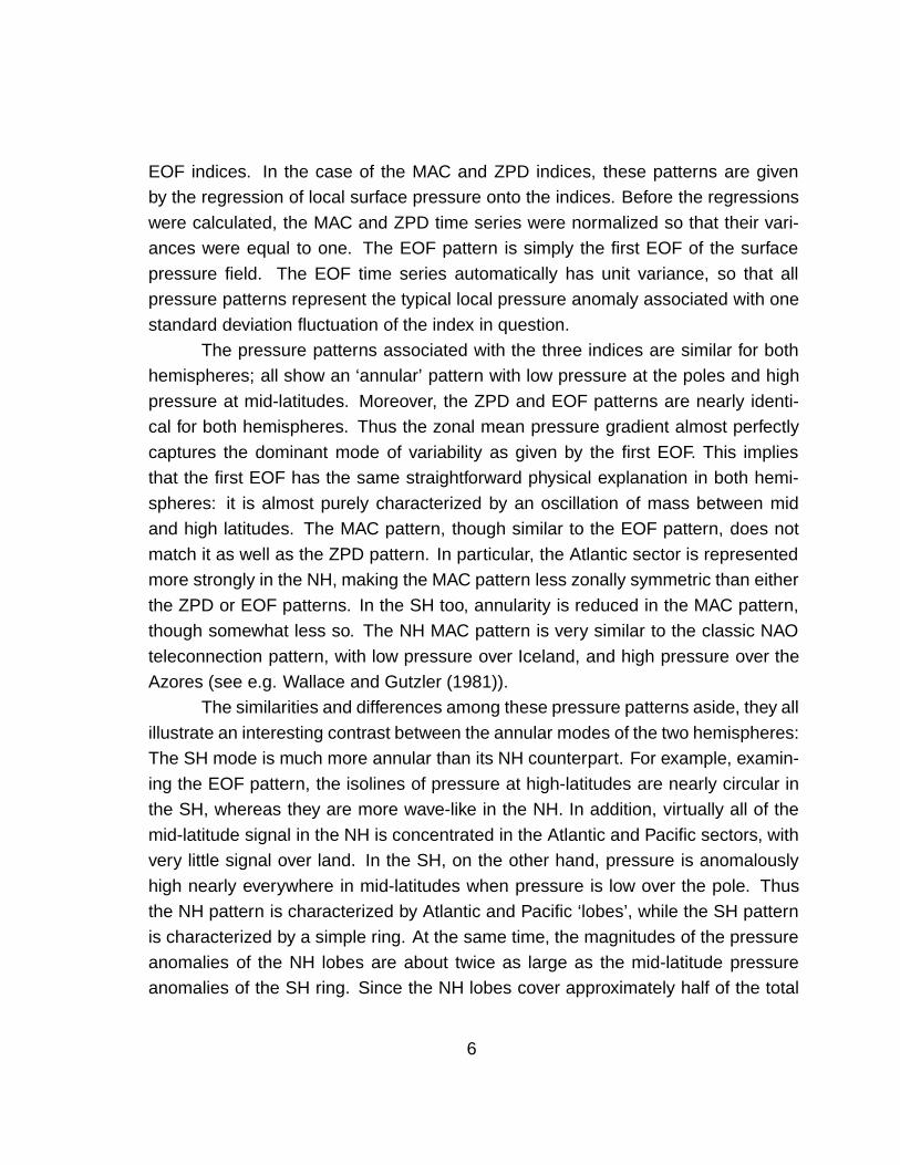
Figure 2: Spectra of MAC and ZPD annular mode indices, calculated using the multi-

taper method. The arrows represent the limits within which 95% of the points lie fora white noise time series with the same variance. Time scales are labeled at the top

of the plot.

area of the mid-latitudes, the total atmospheric mass redistribution associated with

a one standard deviation anomaly of the EOF (or ZPD) index is approximately thesame in both hemispheres. Interestingly, the total variance accounted for by the first

EOF is also approximately the same in both hemispheres (NH=52.7%, SH=52.8%).Thus the annular modes account for about half the pressure field variability in both

hemispheres.The NH and SH EOF patterns of figure 1 are qualitatively similar to the ob-

served patterns, as documented in figure 1 of Thompson and Wallace (1999), whichshows the first EOF of the observed geopotential height field at the lowest levels of

the troposphere. Although observations are sparse, the real SH annular mode isquite zonally symmetric, like the model. In the NH, both observed and modeled pat-

terns exhibit obvious zonal asymmetries, with lobes in the Pacific and Atlantic sec-tors. However, in the observed record, the anomalies of the Pacific lobe are abouthalf as large as the Atlantic lobe, whereas in the model they are approximately equal

in magnitude.

7

Interesting similarities and differences between the NH and SH annular modesare also revealed by examining the spectra of the MAC and ZPD annular mode in-

dices, shown in figure 2. Since the EOF time series are almost perfectly correlatedwith their ZPD counterparts (SH correlation=0.98, NH=0.95), their spectra are not

shown. The spectra of both indices in the NH appear white on time scales longerthan two years. The SH spectra are similar in that they are also nearly white, al-

though the broad peaks around 25 years in both SH indices may be significant. Thevariances of the MAC and ZPD indices agree quite well on all time scales, althoughthe MAC index tends to have slightly more variability. This small difference proba-

bly stems from the fact that the MAC index contains some information about noiseat smaller spatial scales which are filtered out of the ZPD index. In the northern

hemisphere, in contrast, the variances of the two indices do not agree well at all; thevariability of the MAC index is about three times larger than that of the ZPD index.

The reason for this difference between the hemispheres is rooted in the zonal asym-metry of the pressure pattern associated with the NH annular mode (see figure 1).

As noted above, when pressure is anomalously low over the NH pole, high pres-sure is concentrated in the Atlantic and Pacific lobes, whereas when pressure is low

over the SH pole, high pressure is quite uniformly distributed over the mid-latitudes.Thus a pressure anomaly at any SH mid-latitude point tends to reflect quite well the

zonal-mean pressure anomaly. This is much less true in the NH; in the case of theNH MAC index, the mid-latitude point is located in the center of the Atlantic lobe,where the pressure anomaly is much larger than the zonal-mean anomaly. This

significantly enhances the variance of the MAC index compared to the ZPD.While figure 2 reveals that the variability of the MAC index is enhanced in

the NH, it also shows that the overall level of variability of the ZPD index is aboutthe same in the two hemispheres. Thus the variability of the atmospheric mass

re-distribution between mid and high latitudes is approximately the same in bothhemispheres, in spite of the zonal asymmetry of the NH mode. This illustrates one

of the difficulties in interpreting the variability of the MAC index. Comparing the twoMAC spectra, one might be tempted to conclude incorrectly that the NH annular

mode is more vigorous than its SH counterpart.

8

−0.4

−0.3

−0.2

−0.1

−0.2

−0.5

−0.2−0.1 −0

.2

−0.1

−0.8−0.9 −0.9

−0.7

−0.6−0.5

−0.4−0.3

−0.2

−0.6−0.2

−0.1

−0.4−0.2

−0.4

1.5

1

0.5

0

−0.5

10

0.5

0

−0.5

−2−1.5

−1

−2.5

−1.5

−1−1.5

−0.5

0

0

0

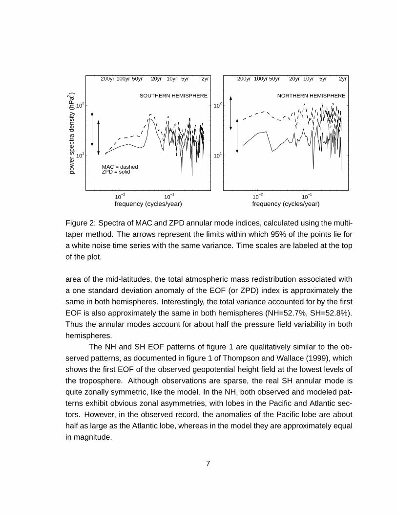
Figure 3: Top left: regression of SAT (�C) onto the time series of the first EOF of thesurface pressure field for NH. Bottom left: same as top left (with the same contours)

except for the SH. Top right: same as bottom left except for the Antarctic regiononly (note that contour intervals are also different). Bottom right: same as top right,except correlation between SAT and the EOF time series is shown.

4 Climatic Impacts

In this section, we examine the climate impacts of the annular modes, focusing

mainly on the poorly understood SH annular mode, but also incorporating somediscussion of the NH for purposes of comparison between the two hemispheres.Throughout this section, we will rely on the EOF index as our annular mode metric.

Choice of this index is somewhat arbitrary; however none of the conclusions wepresent in this section is altered by choosing a different index.

The top left panel of figure 3 shows the regression of surface air temperature

9

(SAT) onto the EOF index for both hemispheres. The NH case exhibits the famil-iar NAO pattern of warming over Eurasia, especially northwestern Europe, cooling

over Newfoundland and southern Greenland, warming over Canada, and coolingcentered over the Bering Sea. It is well-known that this wavenumber two pattern

results mainly from the interaction between the counterclockwise geostrophic flowassociated with the low over the pole (see figure 1) and the land-sea distribution;

warm maritime air is advected over northwestern Europe and Canada, while coldair from the centers of the continents flows to the Bering and Labrador Seas.

The effect of the SH annular mode on SAT is strikingly smaller than in the NH

(figure 3, bottom left panel). The main impact is a modest cooling over Antarctica.Why should the impact on SAT be so much smaller in the SH? We have already

demonstrated (see figure 2) that the variability of the NH and SH ZPD indices isapproximately the same. Thus the magnitudes of the geostrophic wind anomalies

must be about the same in both hemispheres. The difference in the SAT impact isdue to the relative zonal symmetry of the land-sea (and hence mean temperature)

distribution in the SH. Examining the SH EOF pattern of figure 1, it is clear that themost intense geostrophic winds associated with the SH annular mode are located

directly over the circumpolar ocean. Unlike the NH case, these winds do not crossfrom cold land to warm ocean or vice versa, but rather blow continuously across the

ocean. Their impact on local SAT is therefore modest.Since the main impact on SAT is in the Antarctic region, we show a close-up of

the SAT regression over Antarctica and the circumpolar ocean in the top right panel

of figure 3. The entire Antarctic continent cools more than 0.4�C. The greatest cool-ing, reaching values of 0.9�C, is centered over the Ross Sea region. These values

are roughly in line with the analysis of Thompson and Wallace (see figure 9 of theirpaper) based on the sparse SAT observations over Antarctica, although the small

observed warming over the Antarctic Peninsula does not occur in the model. Thevalues are also similar to those obtained by Fyfe et al. (1999), analyzing the Cana-

dian Climate Coupled Model, although they reported results only for November-Aprilaverages (NH winter), rather than during SH winter, when the SH annular mode is

most active. To assess the significance of this SAT signal for the climate of theAntarctic region, we calculated the correlation between SAT and the EOF time se-ries, shown in the bottom right panel of figure 3. The correlations are greater in

10

180oW

120 oW

180oW

0.6 0.6

0.6

0.6

0.60.4

0.4

0.4

0.6

0.2

0

−0.2

0.2−0.2

0−0.2

0.4

120 oW

60

o W

0o

60 oE 1

20o E 180oW

=0.5 cm/s =10 cm/s

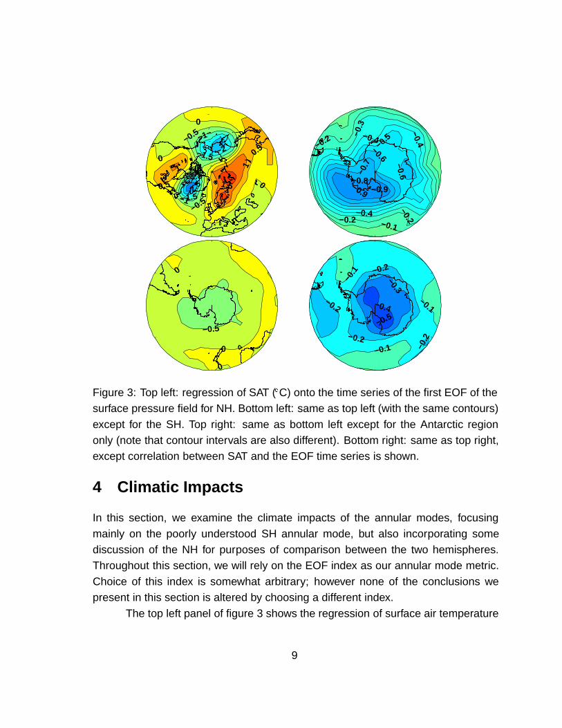
Figure 4: Left: mean JJA currents in the SH ocean poleward of 40�. For clarity, onlyevery other velocity point is plotted. A vector indicating scaling is shown toward the

top of the panel. Middle: regression of JJA surface currents onto the time series ofthe first EOF of the surface pressure field. Note that the scaling vector toward the topof the plot is identical in length to the scaling vector of the left panel but represents a

current 20 times smaller in magnitude. Right: correlation between the v-componentof the JJA surface current and the EOF time series.

magnitude than 0.3 over most of Antarctica, reaching values of 0.5 over the RossSea shelf. Thus although the SH annular mode is a significant contributor to SAT

variability in this region, it is clearly not the only source of SAT variability.While the simulated effects of the SH annular mode on SAT are rather modest

compared to the NH, and account for at most a third to a half of SAT variabilityover Antarctica, the SH annular mode turns out to have significant and interesting

effects on the circumpolar ocean circulation. This possibility is readily apparent byexamining the pressure pattern of the bottom right panel of figure 1. When the SHannular mode is in its positive phase, clockwise geostrophic flow is driven by the

polar low. Because of the nearly-perfect zonal symmetry of the pressure pattern,this creates a nearly uniform zonal wind-stress on the circumpolar ocean. These

surface westerlies, in turn, would drive Ekman pumping to the north in the surfacelayers of the ocean.

To see whether this effect is significant in the model, we analyzed the regres-sion between surface current anomalies and the EOF index, as shown in the middle

panel of figure 4. It is clear that the westerly flow associated with a typical posi-

11

5

10

0

0

5

5

55

−10

−5

−1505

305

0

−20

120 oW

60

o W

0o

60 oE 1

20o E 180oW

−1

−2

−2

−2

−1

2

1

0

−1

31

0

−2

120 oW

60

o W

0o

60 oE 1

20o E 180oW

80oS

−0.4

−0.4

−0.2

0 0.2−0.2

0.4

0.4

0.6

0.20

−0.2

0

0.2 120 o

W

60

o W

0o

60 oE 1

20o E 180oW

80oS

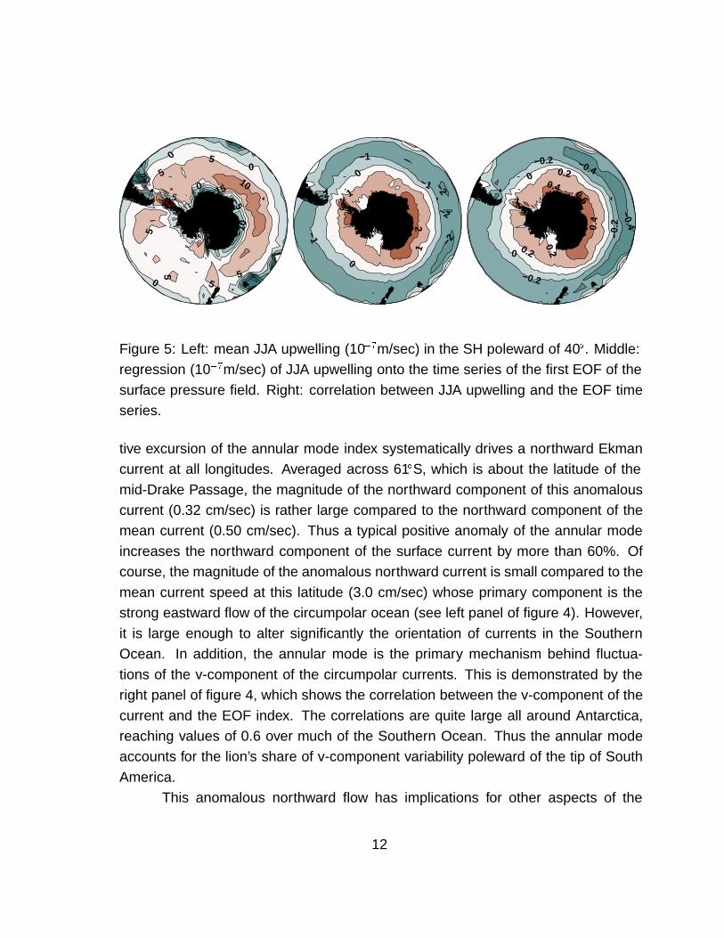
Figure 5: Left: mean JJA upwelling (10�7m/sec) in the SH poleward of 40�. Middle:regression (10�7m/sec) of JJA upwelling onto the time series of the first EOF of the

surface pressure field. Right: correlation between JJA upwelling and the EOF timeseries.

tive excursion of the annular mode index systematically drives a northward Ekmancurrent at all longitudes. Averaged across 61�S, which is about the latitude of the

mid-Drake Passage, the magnitude of the northward component of this anomalouscurrent (0.32 cm/sec) is rather large compared to the northward component of themean current (0.50 cm/sec). Thus a typical positive anomaly of the annular mode

increases the northward component of the surface current by more than 60%. Ofcourse, the magnitude of the anomalous northward current is small compared to the

mean current speed at this latitude (3.0 cm/sec) whose primary component is thestrong eastward flow of the circumpolar ocean (see left panel of figure 4). However,

it is large enough to alter significantly the orientation of currents in the SouthernOcean. In addition, the annular mode is the primary mechanism behind fluctua-

tions of the v-component of the circumpolar currents. This is demonstrated by theright panel of figure 4, which shows the correlation between the v-component of the

current and the EOF index. The correlations are quite large all around Antarctica,reaching values of 0.6 over much of the Southern Ocean. Thus the annular modeaccounts for the lion’s share of v-component variability poleward of the tip of South

America.This anomalous northward flow has implications for other aspects of the

12

ocean circulation. Figure 5 shows the JJA-mean upwelling in the southern ocean(left panel), the regression of JJA upwelling onto the EOF index (middle panel), and

finally, the correlation between JJA upwelling and the EOF index (right panel). Themean upwelling field is characterized by downwelling on the order of 5-15 10�7m/sec

around the coast of Antarctica, and upwelling of around 5 10�7m/sec throughout thecircumpolar ocean. By comparison, the simulated upwelling in the equatorial Pa-

cific, a region where upwelling is particularly intense, averages about 40 10�7m/sec.Thus the typical magnitudes of the upwelling field around Antarctica are not ex-tremely small compared to the rest of the world ocean. A typical positive anomaly

of the EOF index drives an upwelling anomaly around the coast of Antarctica onthe order of 1-2 10�7m/sec (middle panel). It also drives a zonally-symmetric ring

of downwelling of a similar magnitude around the fringes of the circumpolar ocean.Given the horizontal velocity field in the middle panel of figure 4, this vertical circu-

lation is an obvious consequence of mass conservation: The divergent flow aroundAntarctic must be supplied by upwelling, whereas the convergence at the fringes

of the circumpolar ocean must be compensated by downward motion. These up-welling anomalies are rather large (order 20%) compared to the mean values of

the upwelling field. Upwelling variability in this region is also well-correlated withthe annular mode index (right panel). Correlations between 0.4 and 0.7 are seen

around the edges of the Antarctic continent, while anti-correlations less than -0.4are noticeable in the Indian sector of the circumpolar ocean. Thus not only is theannular mode responsible for upwelling anomalies that are rather large compared to

the mean, it also accounts for a great deal of all upwelling variability in this region.The ocean circulation pattern induced by a positive anomaly of the SH annu-

lar mode—upwelling near Antarctica, northward flow across the circumpolar ocean,and downwelling further north—has important implications for the density structure

of the Southern Ocean and the associated geostrophic flow. It is well-known thatthe intense zonal current around Antarctica is sustained by strong meridional tem-

perature (and hence density) gradients. This fact may be understood in terms ofthe thermal wind relation, whereby a meridional density gradient is associated with

a vertical shear of the zonal geostrophic flow. The circulation pattern induced by apositive anomaly of the SH annular mode would intensify the meridional temperaturecontrast across the circumpolar ocean, mainly by injecting relatively warm surface

13

300 400 500 600 700 800 900 100090

95

100

105

110

tran

spor

t (S

v)

400 410 420 430 440 450 460 470 480 490 500−4

−3

−2

−1

0

1

2

3

4

norm

aliz

ed a

nom

aly

mag

nitu

de

model year

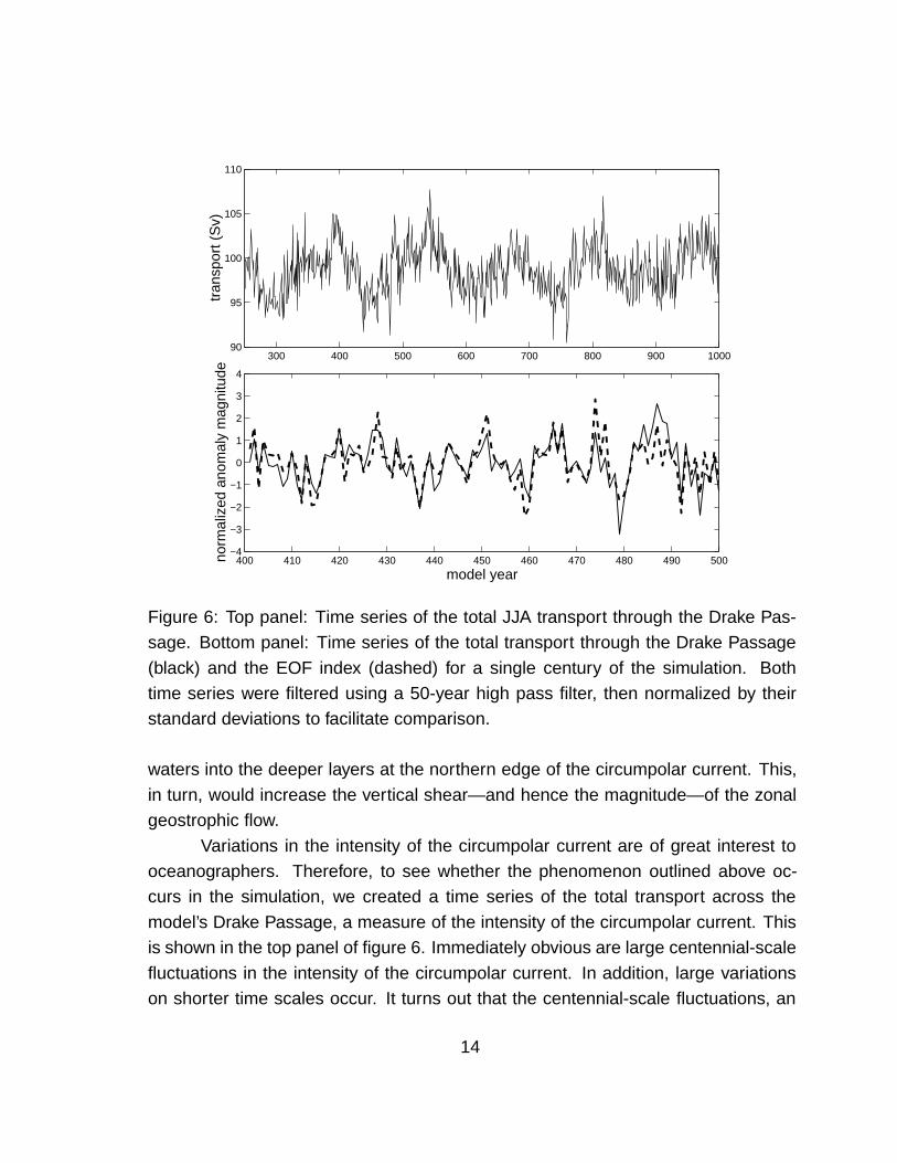
Figure 6: Top panel: Time series of the total JJA transport through the Drake Pas-sage. Bottom panel: Time series of the total transport through the Drake Passage

(black) and the EOF index (dashed) for a single century of the simulation. Bothtime series were filtered using a 50-year high pass filter, then normalized by theirstandard deviations to facilitate comparison.

waters into the deeper layers at the northern edge of the circumpolar current. This,

in turn, would increase the vertical shear—and hence the magnitude—of the zonalgeostrophic flow.

Variations in the intensity of the circumpolar current are of great interest tooceanographers. Therefore, to see whether the phenomenon outlined above oc-curs in the simulation, we created a time series of the total transport across the

model’s Drake Passage, a measure of the intensity of the circumpolar current. Thisis shown in the top panel of figure 6. Immediately obvious are large centennial-scale

fluctuations in the intensity of the circumpolar current. In addition, large variationson shorter time scales occur. It turns out that the centennial-scale fluctuations, an

14

2

10

50

100

200

400

400

200

50

10

2

2

50

120 oW

60

o W

0o

60 oE 1

20o E 180oW

88oS

2.5

5

10

20

2.55

2.5

10

2.5

−10

−5

5 5

−2.5

0

−5

120 oW

60

o W

0o

60 oE 1

20o E 180oW

88oS

0.2

0.15

0.1

−0.25

−0.25

0.20.050

0.1−0.05−

0.1

0.15

0.1

0.1

0.15 0.15

120 oW

60

o W

0o

60 oE 1

20o E 180oW

88oS

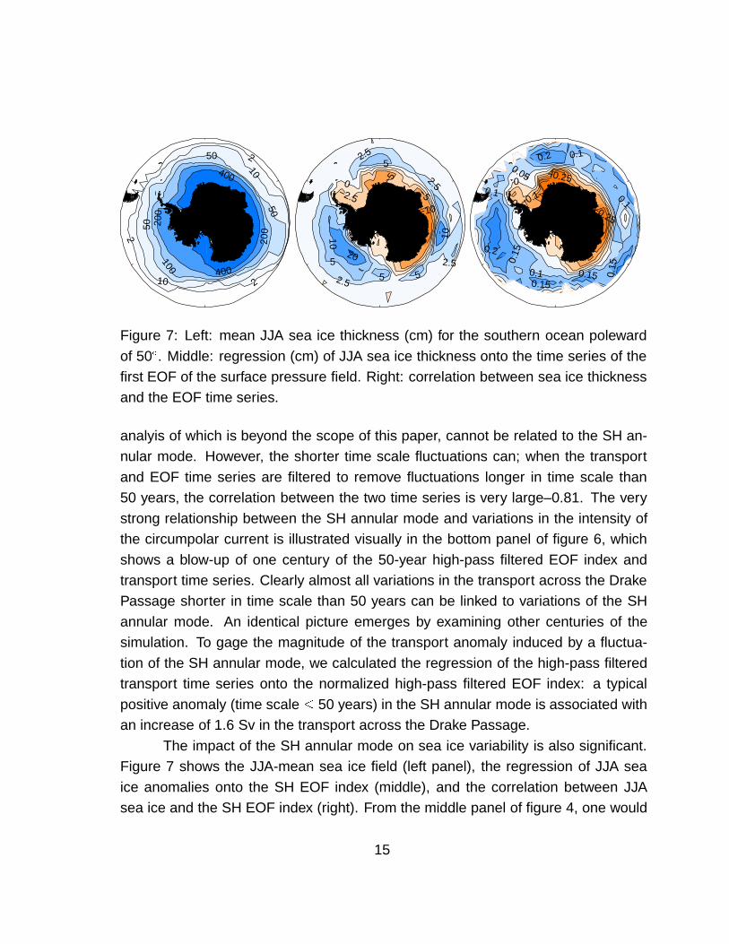
Figure 7: Left: mean JJA sea ice thickness (cm) for the southern ocean poleward

of 50�. Middle: regression (cm) of JJA sea ice thickness onto the time series of thefirst EOF of the surface pressure field. Right: correlation between sea ice thicknessand the EOF time series.

analyis of which is beyond the scope of this paper, cannot be related to the SH an-nular mode. However, the shorter time scale fluctuations can; when the transport

and EOF time series are filtered to remove fluctuations longer in time scale than50 years, the correlation between the two time series is very large–0.81. The very

strong relationship between the SH annular mode and variations in the intensity ofthe circumpolar current is illustrated visually in the bottom panel of figure 6, which

shows a blow-up of one century of the 50-year high-pass filtered EOF index andtransport time series. Clearly almost all variations in the transport across the DrakePassage shorter in time scale than 50 years can be linked to variations of the SH

annular mode. An identical picture emerges by examining other centuries of thesimulation. To gage the magnitude of the transport anomaly induced by a fluctua-

tion of the SH annular mode, we calculated the regression of the high-pass filteredtransport time series onto the normalized high-pass filtered EOF index: a typical

positive anomaly (time scale � 50 years) in the SH annular mode is associated withan increase of 1.6 Sv in the transport across the Drake Passage.

The impact of the SH annular mode on sea ice variability is also significant.Figure 7 shows the JJA-mean sea ice field (left panel), the regression of JJA sea

ice anomalies onto the SH EOF index (middle), and the correlation between JJAsea ice and the SH EOF index (right). From the middle panel of figure 4, one would

15

expect the anomalous northward Ekman current associated with the positive phaseof the SH annular mode to advect ice away from the Antarctic continent toward the

open ocean. The middle panel of figure 7 verifies that this is the case. A decreasein ice thickness on the order of 5 cm is observed around the edges of the continent,

while ice thickness increases of about 5 cm occur at lower latitudes. In some areas,notably in the Pacific sector of the circumpolar ocean, the thickness increases are

larger, reaching 10-20 cm. While the thickness decreases around the edges of thecontinent are not large compared to the very large mean ice thickness there (seeleft panel), the thickness increases over the more thinly covered lower latitudes are

large compared to their mean value. For example, following the 10 cm mean thick-ness contour of the left panel, the thickness anomalies of the middle panel are on

the order of 2.5 to 5 cm. The correlations (right panel) between sea ice anoma-lies and the EOF time series are not large; ice thickness is obviously influenced

by thermodynamic processes as well as advection. However, the correlations aresystematically arranged in a spatially-coherent, ring-like pattern, with maximum anti-

correlation near the continent, and maximum correlation nearer the ice margins. Itshould be noted that the mean ice thicknesses shown in the left panel of figure 7,

are greater than observed: Although the simulated ice thicknesses are constrainedto agree with observed values upon coupling, the model climate drifts so that by the

end of the integration the thicknesses are somewhat larger than observed. However,this does not affect the conclusions presented here; a more realistic ice field wouldrespond in the same way to the Ekman currents associated with the annular mode.

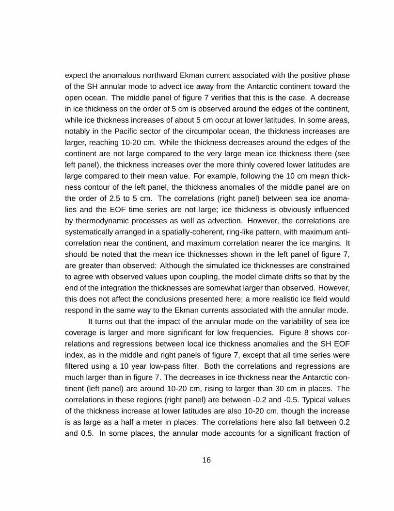
It turns out that the impact of the annular mode on the variability of sea icecoverage is larger and more significant for low frequencies. Figure 8 shows cor-

relations and regressions between local ice thickness anomalies and the SH EOFindex, as in the middle and right panels of figure 7, except that all time series were

filtered using a 10 year low-pass filter. Both the correlations and regressions aremuch larger than in figure 7. The decreases in ice thickness near the Antarctic con-

tinent (left panel) are around 10-20 cm, rising to larger than 30 cm in places. Thecorrelations in these regions (right panel) are between -0.2 and -0.5. Typical values

of the thickness increase at lower latitudes are also 10-20 cm, though the increaseis as large as a half a meter in places. The correlations here also fall between 0.2and 0.5. In some places, the annular mode accounts for a significant fraction of

16

0.4

0.3

0.3

0.3

0.3

0.2

−0.4

−0.3

−0.2

−0.4−0.2

−0.2

00.1

0.2

0.2

0.2

0.2

0.1

−0.3

0

−0.1

−0.2

120 oW

60

o W

0o

60 oE 1

20o E 180oW

88oS

50

40

30

20

10

5

5 1020

5

10

20

30

50

0−5 −10

−20−30

−20

−10

−5

−10−1

0−20

120 oW

60

o W

0o

60 oE 1

20o E 180oW

88oS

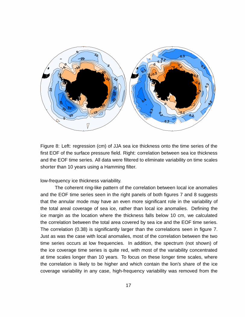
Figure 8: Left: regression (cm) of JJA sea ice thickness onto the time series of the

first EOF of the surface pressure field. Right: correlation between sea ice thicknessand the EOF time series. All data were filtered to eliminate variability on time scales

shorter than 10 years using a Hamming filter.

low-frequency ice thickness variability.The coherent ring-like pattern of the correlation between local ice anomalies

and the EOF time series seen in the right panels of both figures 7 and 8 suggeststhat the annular mode may have an even more significant role in the variability of

the total areal coverage of sea ice, rather than local ice anomalies. Defining theice margin as the location where the thickness falls below 10 cm, we calculatedthe correlation between the total area covered by sea ice and the EOF time series.

The correlation (0.38) is significantly larger than the correlations seen in figure 7.Just as was the case with local anomalies, most of the correlation between the two

time series occurs at low frequencies. In addition, the spectrum (not shown) ofthe ice coverage time series is quite red, with most of the variability concentrated

at time scales longer than 10 years. To focus on these longer time scales, wherethe correlation is likely to be higher and which contain the lion’s share of the ice

coverage variability in any case, high-frequency variability was removed from the

17

300 400 500 600 700 800 900

−3

−2

−1

0

1

2

3

model year

norm

aliz

ed a

nom

aly

mag

nitu

de

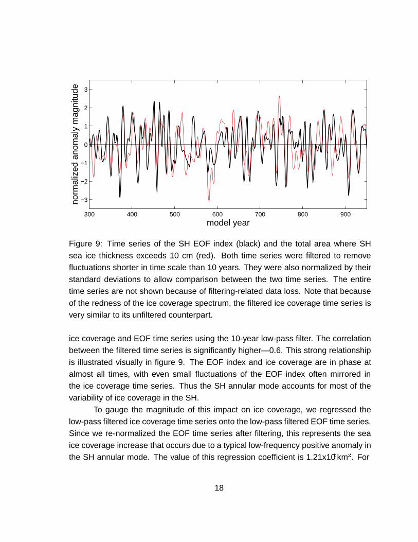
Figure 9: Time series of the SH EOF index (black) and the total area where SH

sea ice thickness exceeds 10 cm (red). Both time series were filtered to removefluctuations shorter in time scale than 10 years. They were also normalized by their

standard deviations to allow comparison between the two time series. The entiretime series are not shown because of filtering-related data loss. Note that because

of the redness of the ice coverage spectrum, the filtered ice coverage time series isvery similar to its unfiltered counterpart.

ice coverage and EOF time series using the 10-year low-pass filter. The correlationbetween the filtered time series is significantly higher—0.6. This strong relationship

is illustrated visually in figure 9. The EOF index and ice coverage are in phase atalmost all times, with even small fluctuations of the EOF index often mirrored inthe ice coverage time series. Thus the SH annular mode accounts for most of the

variability of ice coverage in the SH.To gauge the magnitude of this impact on ice coverage, we regressed the

low-pass filtered ice coverage time series onto the low-pass filtered EOF time series.Since we re-normalized the EOF time series after filtering, this represents the sea

ice coverage increase that occurs due to a typical low-frequency positive anomaly inthe SH annular mode. The value of this regression coefficient is 1.21x106km2. For

18

comparison, the total mean JJA sea ice coverage is 2.88x107km2. Of course, ourdefinition of sea ice margin and hence our measure of sea ice coverage is some-

what arbitrary; however, using other cutoffs gives practically identical answers. Thisdemonstrates that for time scales longer than 10 years, the SH annular mode in-

duces large excursions of the sea ice margin.

5 Summary and Discussion

In section 3, we characterized the wintertime annular modes in this model by exam-

ining MAC, ZPD and EOF indices, their associated surface pressure patterns, andtheir spectra. In both hemispheres, the EOF and ZPD index are almost perfectly

correlated and have nearly identical pressure patterns. This indicates that the firstEOF of surface pressure is almost perfectly described as an oscillation of mass be-

tween mid and high latitudes. However, all three indices show that the mid-latitudepressure distribution of the NH annular mode is concentrated in lobes over the North

Atlantic and Pacific, while in the SH, the distribution is nearly zonally symmetric. Inaddition, in the NH, the most coherent out-of-phase pressure relationship occurs

between Iceland and the Azores, while in the SH, the bias toward any particularlongitude is weaker. Thus the pressure pattern of the NH MAC index is organized

in an NAO-like pattern, with a bias toward the Atlantic sector. For both of thesereasons, the SH annular mode is more ‘annular’ than its NH counterpart. In theserespects the simulated annular modes are similar to the observed annular modes,

except that the Pacific lobe of the simulated NH mode is too intense. The spectra ofthe NH and SH annular modes indices are white. They also show that variability in

the mass distribution between mid and high latitudes is approximately the same inboth hemispheres, in spite of the significant hemispheric differences in the annular

mode pressure patterns.An aquaplanet or a land-only planet would surely have zonally symmetric an-

nular modes at both poles. From this standpoint, the structure of the SH annularmode is easy to understand: the relative zonal symmetry of the land-sea distribution

does little to alter the otherwise zonally symmetric annular mode. It is the NH annu-lar mode that is the oddity in need of further explanation. The Atlantic and Pacificlobe pattern of the NH mode is most likely related to the land-sea distribution and the

19

topography of the land itself. The fact that the most coherent out-of-phase pressurefluctuations occur in the Atlantic sector is probably also related to the land-sea dis-

tribution. This lobe pattern, its bias toward the Atlantic sector, and the availability ofdata led to the concept of the NAO prior to the concept of annular modes. Recently,

Deser (2000) challenged the appropriateness of the annular mode concept for theNH, asserting that the dominance of the Atlantic sector in the NH teleconnection

patterns favors retaining the NAO concept. Of course, the NAO would not exist if theatmosphere did not have a pre-existing tendency for pressure oscillations betweenthe pole and mid-latitudes (i.e. exhibit ‘annular modes’); in this sense, it cannot be

considered a phenomenon independent of the NH’s annular mode. However, it doesseem worthwhile to retain the NAO concept to highlight the anomalous behavior of

the NH annular mode. Why it behaves in this eccentric fashion is also a fascinatingquestion for further study. Perhaps the Pacific sector participates less in the NH

annular mode because the variability there is more affected by tropical influences,such as the ENSO phenomenon.

In section 4, we examined the poorly-known climate implications of the SHannular mode. Compared to the NH, the SAT anomalies associated with the SH

annular mode are small. The difference in the SAT impact is due to the relativezonal symmetry of the land-sea (and hence mean temperature) distribution in the

SH. Unlike the NH case, the geostrophic winds implied by the circular pole-centeredpressure pattern of the SH annular mode do not cross from cold land to warm oceanor vice versa, but rather blow continuously across the ocean or land. Their impact

on local SAT is therefore relatively modest. However, these geostrophic winds dohave significant implications for the ocean. When the annular mode is in a positive

phase (analogous arguments apply for the negative phase), the surface wind stressinduces a northward Ekman current in the upper layer of the circumpolar ocean at

all longitudes. This Ekman pumping explains most of the variability of the circum-polar current’s meridional component. Through mass conservation, this circulation

leads to upwelling near the edge of the Antarctica, and downwelling just north of thecircumpolar current, accounting for much of the upwelling variability in this region.

By altering the meridional temperature gradient, these upwelling and downwellinganomalies lead directly to variations in the intensity of the circumpolar current; whenthe variability due to a centennial-scale oscillation unrelated to the SH annular mode

20

is removed by applying a 50-year high pass filter, the correlation between the SH an-nular mode index and the total transport across the Drake Passage is 0.8. Finally,

this Ekman pumping advects sea ice away from Antarctica, resulting in thinner seaice around the continent, and thicker ice closer to the ice margin. These anomalies

are especially large and significant for variability on time scales longer than 10 years.Because the ice thickness pattern associated with the annular mode is so ring-like,

the annular mode accounts for most of the variability in total areal coverage of seaice; for time scales longer than 10 years, which contain most of the ice coveragevariability, the correlation between the SH annular mode index and ice coverage is

0.6. Thus if a long-term trend were to occur in the SH annular mode—whether an-thropogenic or natural in origin–this could lead to a trend in the ice margin. Why the

SH annular mode does not excite high-frequency excursions of the sea ice marginis an interesting topic for further research.

All of the conclusions presented here regarding the climate impacts of the SHannular mode are for the winter season only. However, unlike its NH counterpart,

the SH annular mode only becomes slightly less active during the other seasonsin both the real world (see Thompson and Wallace 1999) and the present model.

Although a detailed analysis of the climate impacts during other seasons is beyondthe scope of this paper, they are likely to be quite similar to those outlined here, with

the possible exception of the impact on sea ice, which practically disappears duringsummertime.

Of course, the resolution of the model used in this study is relatively coarse.

However, the simulated SH annular mode is quite realistic and the physical mech-anism of the ocean’s response—Ekman pumping driving upwelling anomalies and

fluctuations of the sea ice margin—is exactly what one would expect based on the-oretical understanding of the ocean. It is difficult to see how improved parameter-

izations or increased resolution would alter this picture in any substantial way. Ittherefore seems likely that the actual impacts of the SH annular mode on the ocean

are qualitatively similar to those seen in this simulation.

Acknowledgments.Alex Hall is supported by a Lamont Postdoctoral Fellowship. Martin Visbeck

is supported by NOAA grant XXXXX.

21

References

Bryan K (1969) Climate and the ocean circulation: III. The ocean model. Mon Wea

Rev, 97,806-827.

Bryan K, Lewis L (1979) A water mass model of the world ocean. J Geophys Res,

84(C5), 2503-2517.

Deser C (2000) A note on the annularity of the ‘Arctic Oscillation’. submitted to

Geophys Res Let.

Fyfe, JC, Boer GJ, Flato FM (1999) The Arctic and Antarctic Oscillations and theprojected changes under global warming. Geophys Res Let, 26, 1601-1604.

Kutzbach JE (1970) Large-scale features of monthly-mean northern hemisphereanomaly maps of sea-level pressure. Mon Wea Rev, 98:708-716.

Manabe S, Stouffer RJ, Spelman M, Bryan K (1991) Transient responses of a cou-pled ocean-atmosphere model to gradual changes of atmospheric CO2. Part

I: annual-mean response. J Clim 4:785-817

Marotzke J, Stone P (1995) Atmospheric transports, the thermohaline circulation,

and flux adjustments in a simple coupled model. J Phys Oceanogr 25:1350-1364

Redi MH (1982) Oceanic isopycnal mixing by coordinate rotation. J Phys Oceanogr,12, 1154-1158.

Pacanowski R, Dixon K, Rosati A (1991) The G.F.D.L Modular Ocean Model UsersGuide. GFDL Ocean Group Technical Report 2

Thompson DWJ, Wallace JM (1998) The Arctic Oscillation signature in the winter-time geopotential height and temperature fields. Geophys Res Let, 25:1297-1300.

Thompson DWJ, Wallace JM (1999) Annular Modes in the Extratropical Circulation.Part I: Month-to-month variability. submitted to J Clim.

22

Tziperman E, Bryan K (1993): Estimating global air-sea fluxes from surface prop-erties and from climatological flux data using an oceanic general circulation

model. J Geophys Res, 98(C12), 22629-22644.

Walker GT, Bliss EW (1932) World Weather V. Mem Roy Meteor Soc, 4:53-84.

Wallace JM, Gutzler DS (1981): Teleconnections in the geopotential height fieldduring Northern Hemisphere winter. Mon Wea Rev, 109, 784-812.

23