Annuities - Michigan State...
43
Annuities Lecture: Weeks 9-11 Lecture: Weeks 9-11 (STT 455) Annuities Fall 2014 - Valdez 1 / 43
Transcript of Annuities - Michigan State...

Annuities
Lecture: Weeks 9-11
Lecture: Weeks 9-11 (STT 455) Annuities Fall 2014 - Valdez 1 / 43

What are annuities?
What are annuities?An annuity is a series of payments that could vary according to:
timing of paymentbeginning of year (annuity-due)
time0 1 2 3
1 1 1 1
end of year (annuity-immediate)
time0 1 2 3
1 1 1
with fixed maturityn-year annuity-due
time0 1 2 n-1 n
1 1 1 1
n-year annuity-immediate
time0 1 2 n-1 n
1 1 1 1
more frequently than once a yearannuity-due payable m-thly
time0 1m
2m
1 1 1m
1 2m
2
1m
1m
1m
1m
1m
1m
1m
annuity-immediate payable m-thly
time0 1m
2m
1 1 1m
1 2m
2
1m
1m
1m
1m
1m
1m
payable continuouslycontinuous annuity
time0 1 2 3
1 1 1
varying benefitsLecture: Weeks 9-11 (STT 455) Annuities Fall 2014 - Valdez 2 / 43

What are annuities? annuities-certain
Review of annuities-certain
annuity-due
payable annually
an =
n∑k=0
vk−1 =1− vn
d
payable m times a year
a(m)n =
1
m
mn−1∑k=0
vk/m =1− vn
d(m)
annuity-immediate
an =
n∑k=1
vk =1− vn
i
a(m)n =
1
m
mn∑k=1
vk =1− vn
i(m)
continuous annuity
an =
∫ n
0vtdt =
1− vn
δ
Lecture: Weeks 9-11 (STT 455) Annuities Fall 2014 - Valdez 3 / 43

Chapter summary
Chapter summary
Life annuities
series of benefits paid contingent upon survival of a given life
single life considered
actuarial present values (APV) or expected present values (EPV)
actuarial symbols and notation
Types of annuities
discrete - due or immediate
payable more frequently than once a year
continuous
varying payments
“Current payment techniques” APV formulas
Chapter 5 of Dickson, et al.
Lecture: Weeks 9-11 (STT 455) Annuities Fall 2014 - Valdez 4 / 43
Whole life annuity-due
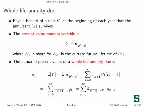
Whole life annuity-due
Pays a benefit of a unit $1 at the beginning of each year that theannuitant (x) survives.
The present value random variable is
Y = aK+1
where K, in short for Kx, is the curtate future lifetime of (x).
The actuarial present value of a whole life annuity-due is
ax = E[Y ] = E[aK+1
]=∞∑k=0
ak+1
Pr[K = k]
=∞∑k=0
ak+1· qk| x =
∞∑k=0
ak+1· pk x qx+k
Lecture: Weeks 9-11 (STT 455) Annuities Fall 2014 - Valdez 5 / 43

Whole life annuity-due current payment technique
Current payment techniqueBy writing the PV random variable as
Y = I(T > 0) + vI(T > 1) + v2I(T > 2) + · · · =∞∑k=0
vkI(T > k),
one can immediately deduce that
ax = E[Y ] = E
[ ∞∑k=0
vkI(T > k)
]
=
∞∑k=0
vkE[I(T > k)] =
∞∑k=0
vkPr[I(T > k)]
=
∞∑k=0
vk pk x =
∞∑k=0
Ek x =
∞∑k=0
A 1x: k
.
A straightforward proof of∞∑k=0
ak+1· qk| x =
∞∑k=0
vk pk x is in Exercise 5.1.
Lecture: Weeks 9-11 (STT 455) Annuities Fall 2014 - Valdez 6 / 43

Whole life annuity-due - continued
Current payment technique - continued
The commonly used formula ax =
∞∑k=0
vk pk x is the so-called current
payment technique for evaluating life annuities.
Indeed, this formula gives us another intuitive interpretation of whatlife annuities are: they are nothing but sums of pure endowments(you get a benefit each time you survive).
The primary difference lies in when you view the payments: one givesthe series of payments made upon death, the other gives the paymentmade each time you survive.
Lecture: Weeks 9-11 (STT 455) Annuities Fall 2014 - Valdez 7 / 43

Whole life annuity-due some useful formulas
Some useful formulas
By recalling that aK+1
=1− vK+1
d, we can use this to derive:
relationship to whole life insurance
ax = E
[1− vK+1
d
]=
1
d(1−Ax) .
Alternatively, we write: Ax = 1− dax. very important formula!
the variance formula
Var[Y ] = Var[aK+1
]=
1
d2Var
[vK+1
]=
1
d2
[A2 x − (Ax)2
].
Lecture: Weeks 9-11 (STT 455) Annuities Fall 2014 - Valdez 8 / 43

Whole life annuity-due illustrative example
Illustrative example 1
Suppose you are interested in valuing a whole life annuity-due issued to(95). You are given:
i = 5%, and
the following extract from a life table:
x 95 96 97 98 99 100
`x 100 70 40 20 4 0
1 Express the present value random variable for a whole life annuity-dueto (95).
2 Calculate the expected value of this random variable.
3 Calculate the variance of this random variable.
Lecture: Weeks 9-11 (STT 455) Annuities Fall 2014 - Valdez 9 / 43
Other types temporary life annuity-due
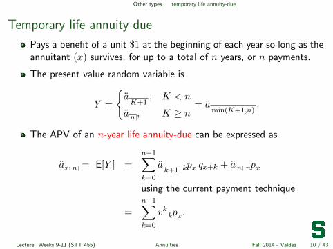
Temporary life annuity-due
Pays a benefit of a unit $1 at the beginning of each year so long as theannuitant (x) survives, for up to a total of n years, or n payments.
The present value random variable is
Y =
{aK+1
, K < n
an , K ≥ n= a
min(K+1,n).
The APV of an n-year life annuity-due can be expressed as
ax:n = E[Y ] =
n−1∑k=0
ak+1
pk x qx+k + an pn x
using the current payment technique
=
n−1∑k=0
vk pk x.
Lecture: Weeks 9-11 (STT 455) Annuities Fall 2014 - Valdez 10 / 43

Other types some useful formulas
Some useful formulas
Notice that Z = vmin(K+1,n) is the PV random variable associated with ann-year endowment insurance, with death benefit payable at EOY. Similarto the case of the whole life, we can use this to derive:
relationship to whole life insurance
ax:n = E
[1− Zd
]=
1
d
(1− Ax:n
).
Alternatively, we write: Ax:n = 1− dax:n . very important formula!
the variance formula
Var[Y ] =1
d2Var[Z] =
1
d2
[A2 x:n −
(Ax:n
)2].
Lecture: Weeks 9-11 (STT 455) Annuities Fall 2014 - Valdez 11 / 43

Other types deferred whole life annuity-due
Deferred whole life annuity-due
Pays a benefit of a unit $1 at the beginning of each year while theannuitant (x) survives from x+ n onward.
The PV random variable can be expressed in a number of ways:
Y =
{0, 0 ≤ K < n
an| K+1−n = vna
K+1−n = aK+1
− an , K ≥ n .
The APV of an n-year deferred whole life annuity can be expressed as
an| x = E[Y ] =
∞∑k=n
vk pk x
= En x ax+n = ax − ax:n .
Lecture: Weeks 9-11 (STT 455) Annuities Fall 2014 - Valdez 12 / 43

Other types variance formula
Variance of a deferred whole life annuity-dueTo derive the variance is not straightforward. The best strategy is to workwith
Y =
{0, 0 ≤ K < n
vn aK+1−n , K ≥ n
and use
Var[Y ] = E[Y 2]− (E[Y ])2
=
∞∑k=n
v2n(ak+1−n
)2qk| x −
(an| x
)2Apply a change of variable of summation to say k∗ = k − n and then thevariance of a whole life insurance issued to (x+ n).
The variance of Y finally can be expressed as
Var[Y ] =2
dv2n pn x
(ax+n − a2 x+n
)+ a2n| x −
(an| x
)2.
Lecture: Weeks 9-11 (STT 455) Annuities Fall 2014 - Valdez 13 / 43

Other types illustrative example
Illustrative example 2
Suppose you are interested in valuing a 2-year deferred whole lifeannuity-due issued to (95). You are given:
i = 6% and
the following extract from a life table:
x 95 96 97 98 99 100
`x 1000 750 400 225 75 0
1 Express the present value random variable for this annuity.
2 Calculate the expected value of this random variable.
3 Calculate the variance of this random variable.
Lecture: Weeks 9-11 (STT 455) Annuities Fall 2014 - Valdez 14 / 43

Other types recursive relationships
Recursive relationships
The following relationships are easy to show:
ax = 1 + vpxax+1 = 1 + E1 x ax+1
= 1 + vpx + v2 p2 xax+2 = 1 + E1 x + E2 x ax+2
In general, because E’s are multiplicative, we can generalized thisrecursions to
ax =
∞∑k=0
Ek x =
n−1∑k=0
Ek x +
∞∑k=n
Ek x
apply change of variable k∗ = k − n
= ax:n +
∞∑k∗=0
En x Ek∗ x+n = ax:n + En x
∞∑k∗=0
Ek∗ x+n
= ax:n + En x ax+n = ax:n + an| x
The last term shows that a whole life annuity is the sum of a term lifeannuity and a deferred life annuity.
Lecture: Weeks 9-11 (STT 455) Annuities Fall 2014 - Valdez 15 / 43

Other types parameter sensitivity
20 40 60 80 100
1020
30
40
50
x
ax
i = 1%i = 5%i = 10%i = 15%i = 20%
20 40 60 80 100
510
15
20
x
ax
c = 1.124c = 1.130c = 1.136c = 1.142c = 1.148
Figure : Comparing APV of a whole life annuity-due for based on the StandardUltimate Survival Model (Makeham with A = 0.00022, B = 2.7× 10⁻⁶,c = 1.124). Left figure: varying i. Right figure: varying c with i = 5%
Lecture: Weeks 9-11 (STT 455) Annuities Fall 2014 - Valdez 16 / 43

Life annuity-immediate whole life
Whole life annuity-immediate
Procedures and principles for annuity-due can be adapted forannuity-immediate.
Consider the whole life annuity-immediate, the PV random variable isclearly Y = a
Kso that APV is given by
ax = E[Y ] =
∞∑k=0
aK· pk x qx+k =
∞∑k=1
vk pk x.
Relationship to life insurance:
Y =1
i
(1− vK
)=
1
i
[1− (1 + i)vK+1
]leads to 1 = iax + (1 + i)Ax.
Interpretation of this equation - to be discussed in class.
Lecture: Weeks 9-11 (STT 455) Annuities Fall 2014 - Valdez 17 / 43

Life annuity-immediate other types
Other types of life annuity-immediate
For an n-year life annuity-immediate:
Find expression for the present value random variable.
Express formulas for its actuarial present value or expectation.
Find expression for the variance of the present value random variable.
For an n-year deferred whole life annuity-immediate:
Find expression for the present value random variable.
Give expressions for the actuarial present value.
Details to be discussed in lecture.
Lecture: Weeks 9-11 (STT 455) Annuities Fall 2014 - Valdez 18 / 43

Life annuities with m-thly payments
Life annuities with m-thly payments
In practice, life annuities are often payable more frequently than once ayear, e.g. monthly (m = 12), quarterly (m = 4), or semi-annually(m = 2).
Here, we define the random variable K(m)x , or simply K(m), to be the
complete future lifetime rounded down to the nearest 1/m-th of a year.
For example, if the observed T = 45.86 for a life (x) and m = 4, then theobserved K(4) is 453
4 .
Indeed, we can write
K(m) =1
mbmT c ,
where b c is greatest integer (or floor) function.
Lecture: Weeks 9-11 (STT 455) Annuities Fall 2014 - Valdez 19 / 43

Life annuities with m-thly payments whole life annuity-due
Whole life annuity-due payable m times a year
Consider a whole life annuity-due with payments made m times ayear. Its PV random variable can be expressed as
Y = a(m)
K(m)+(1/m)=
1− vK(m)+(1/m)
d(m).
The APV of this annuity is
E[Y ] = a(m)x =
1
m
∞∑h=0
vh/m · ph/m x =1−A(m)
x
d(m).
Variance is
Var[Y ] =Var
[vK
(m)+(1/m)]
(d(m)
)2 =A
2 (m)x −
(A
(m)x
)2(d(m)
)2 .
Lecture: Weeks 9-11 (STT 455) Annuities Fall 2014 - Valdez 20 / 43

Life annuities with m-thly payments some useful relationships
Some useful relationships
Here we list some important relationships regarding the life annuity-duewith m-thly payments (Note - these are exact formulas):
1 = dax +Ax = d(m)a(m)x +A
(m)x
a(m)x =
d
d(m)ax −
1
d(m)
(A
(m)x −Ax
)= a
(m)
1ax − a(m)
∞
(A
(m)x −Ax
)
a(m)x =
1−A(m)x
d(m)= a
(m)∞ − a
(m)∞ A
(m)x
Lecture: Weeks 9-11 (STT 455) Annuities Fall 2014 - Valdez 21 / 43

Life annuities with m-thly payments other types
Other types of life annuity-due payable m-thly
n-year term PV random variable Y = a(m)
min(K(m)+(1/m),n)
APV symbol E[Y ] = a(m)x:n
current payment technique =1
m
mn−1∑h=0
vh/m · ph/m x
other relationships = a(m)x − En x a
(m)x+n
relation to life insurance =1
d(m)
[1−A(m)
x:n
]
n-year deferred PV random variable Y = vna(m)
K(m)+(1/m)−nI(K ≥ n)
APV symbol E[Y ] = a(m)
n| x
current payment technique =1
m
∞∑h=mn
vh/m · ph/m x
other relationships = En x a(m)x+n = a
(m)x − a(m)
x:n
relation to life insurance =1
d(m)
[En x − A
(m)n| x
]
Lecture: Weeks 9-11 (STT 455) Annuities Fall 2014 - Valdez 22 / 43
Life annuities with m-thly payments illustrative example
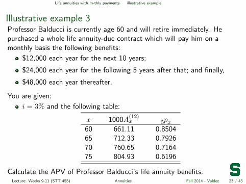
Illustrative example 3Professor Balducci is currently age 60 and will retire immediately. Hepurchased a whole life annuity-due contract which will pay him on amonthly basis the following benefits:
$12,000 each year for the next 10 years;
$24,000 each year for the following 5 years after that; and finally,
$48,000 each year thereafter.
You are given:
i = 3% and the following table:
x 1000A(12)x p5 x
60 661.11 0.850465 712.33 0.792670 760.65 0.716475 804.93 0.6196
Calculate the APV of Professor Balducci’s life annuity benefits.Lecture: Weeks 9-11 (STT 455) Annuities Fall 2014 - Valdez 23 / 43

Continuous whole life annuity
(Continuous) whole life annuity
A life annuity payable continuously at the rate of one unit per year.
One can think of it as life annuity payable m-thly per year, withm→∞.
The PV random variable is Y = aT
where T is the future lifetime of
(x).
The APV of the annuity:
ax = E[Y ] = E[aT
]=
∫ ∞0
at· pt xµx+tdt
use integration by parts - see page 117 for proof
=
∫ ∞0
vt pt xdt =
∫ ∞0
Et xdt
Lecture: Weeks 9-11 (STT 455) Annuities Fall 2014 - Valdez 24 / 43

Continuous whole life annuity
- continued
One can also write expressions for the cdf and pdf of Y in terms ofthe cdf and pdf of T . For example,
Pr[Y ≤ y] = Pr[1− vT ≤ δy
]= Pr
[T ≤ log(1− δy)
log v
]Recursive relation: ax = a
x: 1+ vpxax+1
Variance expression: Var[aT
]= Var
[1− vT
δ
]=
1
δ2
[A2 x −
(Ax
)2]Relationship to whole life insurance: Ax = 1− δax
Try writing explicit expressions for the APV and variance where wehave constant force of mortality and constant force of interest.
Lecture: Weeks 9-11 (STT 455) Annuities Fall 2014 - Valdez 25 / 43

Continuous temporary life annuity
Temporary life annuity
A (continuous) n-year temporary life annuity pays 1 per yearcontinuously while (x) survives during the next n years.
The PV random variable is Y =
{aT, 0 ≤ T < n
an , T ≥ n= a
min(T,n)
The APV of the annuity:
ax:n = E[Y ] =
∫ n
0at· pt xµx+tdt
+
∫ ∞n
an · pt xµx+tdt =
∫ n
0vt pt xdt.
Recursive formula: ax:n = ax: 1
+ vpx ax+1:n−1 .
To derive variance, one way to get explicit form is to note thatY = (1− Z) /δ where Z is the PV r.v. for an n-year endowment ins.[details in class.]
Lecture: Weeks 9-11 (STT 455) Annuities Fall 2014 - Valdez 26 / 43

Continuous deferred whole life annuity
Deferred whole life annuity
Pays a benefit of a unit $1 each year continuously while the annuitant(x) survives from x+ n onward.
The PV random variable is
Y =
{0, 0 ≤ T < n
vn aT−n , T ≥ n
=
{0, 0 ≤ T < n
aT− an , T ≥ n
.
The APV [expected value of Y ] of the annuity is
an| x = En x ax = ax − ax:n =
∫ ∞n
vt pt xdt.
The variance of Y is given by
Var[Y ] =2
δv2n pn x
(ax+n − a2 x+n
)−(
an| x
)2Lecture: Weeks 9-11 (STT 455) Annuities Fall 2014 - Valdez 27 / 43

Continuous special mortality laws
Special mortality laws
Just as in the case of life insurance valuation, we can derive niceexplicit forms for “life annuity” formulas in the case where mortalityfollows:
constant force (or Exponential distribution); or
De Moivre’s law (or Uniform distribution).
Try deriving some of these formulas. You can approach them in acouple of ways:
Know the results for the “life insurance” case, and then use therelationships between annuities and insurances.
You can always derive it from first principles, usually working with thecurrent payment technique.
In the continuous case, one can use numerical approximations toevaluate the integral:
trapezium (trapezoidal) rule
repeated Simpson’s rule
Lecture: Weeks 9-11 (STT 455) Annuities Fall 2014 - Valdez 28 / 43

Other forms varying benefits
Life annuities with varying benefits
Some of these are discussed in details in Section 5.10.
You may try to remember the special symbols used, especially if thevariation is a fixed unit of $1 (either increasing or decreasing).
The most important thing to remember is to apply similar concept of“discounting with life” taught in the life insurance case (note: thisworks only for valuing actuarial present values):
work with drawing the benefit payments as a function of time; and
use then your intuition to derive the desired results.
Lecture: Weeks 9-11 (STT 455) Annuities Fall 2014 - Valdez 29 / 43

Evaluating annuities
Methods for evaluating annuity functions
Section 5.11
Recursions:
For example, in the case of a whole life annuity-due on (x), recallax = 1 + vpxax+1. Given a set of mortality assumptions, start with
ax =
∞∑k=0
vk pk x
and then use the recursion to evaluate values for subsequent ages.
UDD: deaths are uniformly distribution between integral ages.
Woolhouse’s approximations
Lecture: Weeks 9-11 (STT 455) Annuities Fall 2014 - Valdez 30 / 43

Evaluating annuities UDD
Uniform Distribution of Deaths (UDD)Under the UDD assumption, we have derived in the previous chapter thatthe following holds:
A(m)x =
i
i(m)Ax
Then use the relationship between annuities and insurance:
a(m)x =
1−A(m)x
d(m)
This leads us to the following result when UDD holds:
a(m)x = α (m) ax − β (m) ,
where
α (m) = s(m)
1a(m)
1=
i
i(m)· d
d(m)
β (m) =s(m)
1− 1
d(m)=
i− i(m)
i(m)d(m)
Lecture: Weeks 9-11 (STT 455) Annuities Fall 2014 - Valdez 31 / 43

Evaluating annuities Woolhouse’s formulas
Woolhouse’s approximate fomulas
The Woolhouse’s approximate formulas for evaluating annuities are basedon the Euler-Maclaurin formula for numerical integration:∫ ∞
0g(t)dt = h
∞∑k=0
g(kh)− h
2g(0) +
h2
12g′(0)− h4
720g′′(0) + · · ·
for some positive constant h. This formula is then applied to g(t) = vt pt x
which leads us tog′(t) = −vt pt x (δ − µx+t) .
We can obtain the following Woolhouse’s approximate formula:
a(m)x ≈ ax −
m− 1
2m− m2 − 1
12m2(δ + µx)
Lecture: Weeks 9-11 (STT 455) Annuities Fall 2014 - Valdez 32 / 43

Evaluating annuities Woolhouse’s formulas
Approximating an n-year temporary life annuity-due withm-thly paymentsApply the Woolhouse’s approximate formula to
a(m)x:n = a(m)
x − En x a(m)x+n
This leads us to the following Woolhouse’s approximate formulas:
Use 2 terms (W2) a(m)x:n ≈ ax:n −
m−12m (1− En x)
Use 3 terms (W3) a(m)x:n ≈ ax:n −
m−12m (1− En x)
−m2−112m2 [δ + µx − En x (δ + µx+n)]
Use 3 terms (W3*) use approximation for force of mortality
(modified) µx ≈ −12 [log(px−1) + log(px)]
Lecture: Weeks 9-11 (STT 455) Annuities Fall 2014 - Valdez 33 / 43

Woolhouse’s formulas numerical illustrations
Numerical illustrations
We compare the various approximations: UDD, W2, W3, W3* based onthe Standard Ultimate Survival Model with Makeham’s law
µx = A+Bcx,
where A = 0.00022, B = 2.7× 10⁻⁶ and c = 1.124.
The results for comparing the values for:
a(12)
x: 10with i = 10%
a(2)
x: 25with i = 5%
are summarized in the following slides.
Lecture: Weeks 9-11 (STT 455) Annuities Fall 2014 - Valdez 34 / 43

Woolhouse’s formulas numerical illustrations
Values of a(12)
x: 10with i = 10%
x ax a(12)x E10 x Exact UDD W2 W3 W3*
20 10.9315 10.4653 0.384492 6.4655 6.4655 6.4704 6.4655 6.465530 10.8690 10.4027 0.384039 6.4630 6.4630 6.4679 6.4630 6.463040 10.7249 10.2586 0.382586 6.4550 6.4550 6.4599 6.4550 6.455050 10.4081 9.9418 0.377947 6.4295 6.4294 6.4344 6.4295 6.429560 9.7594 9.2929 0.363394 6.3485 6.3482 6.3535 6.3485 6.348570 8.5697 8.1027 0.320250 6.0991 6.0982 6.1044 6.0990 6.099080 6.7253 6.2565 0.213219 5.4003 5.3989 5.4073 5.4003 5.400390 4.4901 4.0155 0.057574 3.8975 3.8997 3.9117 3.8975 3.8975
100 2.5433 2.0505 0.000851 2.0497 2.0699 2.0842 2.0497 2.0496
Lecture: Weeks 9-11 (STT 455) Annuities Fall 2014 - Valdez 35 / 43

Woolhouse’s formulas numerical illustrations
Values of a(2)
x: 25with i = 5%
x ax a(2)x E25 x Exact UDD W2 W3 W3*
20 19.9664 19.7133 0.292450 14.5770 14.5770 14.5792 14.5770 14.577030 19.3834 19.1303 0.289733 14.5506 14.5505 14.5527 14.5506 14.550640 18.4578 18.2047 0.281157 14.4663 14.4662 14.4684 14.4663 14.466350 17.0245 16.7714 0.255242 14.2028 14.2024 14.2048 14.2028 14.202860 14.9041 14.6508 0.186974 13.4275 13.4265 13.4295 13.4275 13.427570 12.0083 11.7546 0.068663 11.5117 11.5104 11.5144 11.5117 11.511780 8.5484 8.2934 0.002732 8.2889 8.2889 8.2938 8.2889 8.288990 5.1835 4.9242 0.000000 4.9242 4.9281 4.9335 4.9242 4.9242
100 2.7156 2.4425 0.000000 2.4425 2.4599 2.4656 2.4424 2.4424
Lecture: Weeks 9-11 (STT 455) Annuities Fall 2014 - Valdez 36 / 43

Woolhouse’s formulas visualizing the differences
20 27 34 41 48 55 62 69 76 83 90 97
age x
Exa
ctminus
UDD
-0.020
-0.010
0.00
0
20 27 34 41 48 55 62 69 76 83 90 97
age x
Exa
ctminus
W2
-0.025
-0.015
-0.005
20 27 34 41 48 55 62 69 76 83 90 97
age x
Exa
ctminus
W3
-0.002
-0.001
0.00
00.00
10.00
2
20 27 34 41 48 55 62 69 76 83 90 97
age x
Exa
ctminus
W3*
-0.002
-0.001
0.00
00.00
10.00
2
Figure : Visualizing the different approximations for a(2)
x: 25Lecture: Weeks 9-11 (STT 455) Annuities Fall 2014 - Valdez 37 / 43

Woolhouse’s formulas illustrative example
Illustrative example 4You are given:
i = 5% and the following table:
x `x µx49 811 0.021350 793 0.023551 773 0.025852 753 0.028453 731 0.031254 707 0.0344
Approximate a(12)
50: 3based on the following methods:
1 UDD assumptions2 Woolhouse’s formula using the first two terms only3 Woolhouse’s formula using all three terms4 Woolhouse’s formula using all three terms but approximating the
force of mortality
Lecture: Weeks 9-11 (STT 455) Annuities Fall 2014 - Valdez 38 / 43

Additional practice problems
Practice problem 1
You are given:
`x = 115− x, for 0 ≤ x ≤ 115
δ = 4%
Calculate a65: 20
.
Lecture: Weeks 9-11 (STT 455) Annuities Fall 2014 - Valdez 39 / 43

Additional practice problems
Practice problem 2
You are given:
µx+t = 0.03, for t ≥ 0
δ = 5%
Y is the present value random variable for a continuous whole lifeannuity of $1 issued to (x).
Calculate Pr
[Y ≥ E[Y ]−
√Var[Y ]
].
Lecture: Weeks 9-11 (STT 455) Annuities Fall 2014 - Valdez 40 / 43

Additional practice problems
Practice problem 3 - modified SOA MLC Spring 2012
For a whole life annuity-due of $1,000 per year on (65), you are given:
Mortality follows Gompertz law with
µx = Bcx, for x ≥ 0,
where B = 5× 10⁻⁵ and c = 1.1.
i = 4%
Y is the present value random variable for this annuity.
Calculate the probability that Y is less than $11,500.
Lecture: Weeks 9-11 (STT 455) Annuities Fall 2014 - Valdez 41 / 43

Additional practice problems
Practice problem 4 - SOA MLC Spring 2014
For a group of 100 lives age x with independent future lifetimes, you aregiven:
Each life is to be paid $1 at the beginning of each year, if alive.
Ax = 0.45
A2 x = 0.22
i = 0.05
Y is the present value random variable of the aggregate payments.
Using the Normal approximation to Y , calculate the initial size of the fundneeded in order to be 95% certain of being able to make the payments forthese life annuities.
Lecture: Weeks 9-11 (STT 455) Annuities Fall 2014 - Valdez 42 / 43

Other terminologies
Other terminologies and notations used
Expression Other terms/symbols used
temporary life annuity-dueterm annuity-duen-year term life annuity-due
annuity-immediateimmediate annuityannuity immediate
Lecture: Weeks 9-11 (STT 455) Annuities Fall 2014 - Valdez 43 / 43