Anisotropic Hydrodynamic Parameters of Regenerator...
9
Anisotropic Hydrodynamic Parameters of Regenerator Materials Suitable for Miniature Cryocoolers T.J. Conrad 1 , E.C. Landrum 1 , S.M. Ghiaasiaan 1 , C.S. Kirkconnell 2 , T. Crittenden 3 , and S. Yorish 3 1 Georgia Institute of Technology, Atlanta, GA 30332 2 Raytheon SAS, El Segundo, CA 90245 3 Virtual AeroSurface Technologies, Atlanta, GA 30318 ABSTRACT Recent successful CFD models of cryocooler systems have shown that such models can pro- vide very useful performance predictions for cryocoolers. For miniature cryocoolers, CFD model- ing is likely the best technique available as models developed for larger systems may not accurately represent phenomena which become important as the device scale is reduced. Accurate CFD mod- eling of Stirling and pulse tube refrigerators requires realistic closure relations, particularly with respect to the hydrodynamic and thermal transport processes for the porous media which make up their heat exchangers and regenerators. Generally, these porous media are morphologically aniso- tropic, and thus the parameters which characterize them are anisotropic as well. Measurement of the hydrodynamic parameters in at least two dimensions is therefore preferred. Miniature regenerative cryocoolers will require porous regenerator and heat exchanger fillers with considerably smaller characteristic pore sizes than those commonly used in larger scale de- vices. This paper describes measurements of the hydrodynamic parameters of stacked discs of 635 mesh stainless steel and 325 mesh phosphor bronze using a CFD-assisted methodology. These materials are among the finest commercially available structures and can be suitable for use as miniature regenerator and heat exchanger fillers. Measurements were made in the axial and radial directions for both steady and oscillatory flow. Higher frequency operation is preferred for minia- ture cryocoolers; therefore a frequency range between 50 and 200 Hz was investigated for the oscillatory flow cases. The test setups for steady flow incorporated static pressure transducers and a mass flow rate meter; for oscillatory flow, the apparatus included dynamic pressure transducers and hot wire probes for CFD model verification. These test setups were each modeled using the Fluent CFD code. The directional Darcy permeability and Forchheimer’s inertial coefficients were obtained based on iterative comparisons between experimental measurements and CFD simulation results. INTRODUCTION Computational fluid dynamics (CFD) modeling of pulse tube refrigerators requires realistic closure relations, particularly with respect to the hydrodynamic and thermal transport processes for 343
Transcript of Anisotropic Hydrodynamic Parameters of Regenerator...

Anisotropic Hydrodynamic Parametersof Regenerator Materials Suitablefor Miniature Cryocoolers
T.J. Conrad1, E.C. Landrum1, S.M. Ghiaasiaan1, C.S. Kirkconnell2,
T. Crittenden3, and S. Yorish3
1Georgia Institute of Technology, Atlanta, GA 303322Raytheon SAS, El Segundo, CA 902453Virtual AeroSurface Technologies, Atlanta, GA 30318
ABSTRACT
Recent successful CFD models of cryocooler systems have shown that such models can pro-
vide very useful performance predictions for cryocoolers. For miniature cryocoolers, CFD model-
ing is likely the best technique available as models developed for larger systems may not accurately
represent phenomena which become important as the device scale is reduced. Accurate CFD mod-
eling of Stirling and pulse tube refrigerators requires realistic closure relations, particularly with
respect to the hydrodynamic and thermal transport processes for the porous media which make up
their heat exchangers and regenerators. Generally, these porous media are morphologically aniso-
tropic, and thus the parameters which characterize them are anisotropic as well. Measurement of
the hydrodynamic parameters in at least two dimensions is therefore preferred.
Miniature regenerative cryocoolers will require porous regenerator and heat exchanger fillers
with considerably smaller characteristic pore sizes than those commonly used in larger scale de-
vices. This paper describes measurements of the hydrodynamic parameters of stacked discs of
635 mesh stainless steel and 325 mesh phosphor bronze using a CFD-assisted methodology. These
materials are among the finest commercially available structures and can be suitable for use as
miniature regenerator and heat exchanger fillers. Measurements were made in the axial and radial
directions for both steady and oscillatory flow. Higher frequency operation is preferred for minia-
ture cryocoolers; therefore a frequency range between 50 and 200 Hz was investigated for the
oscillatory flow cases. The test setups for steady flow incorporated static pressure transducers and
a mass flow rate meter; for oscillatory flow, the apparatus included dynamic pressure transducers
and hot wire probes for CFD model verification. These test setups were each modeled using the
Fluent CFD code. The directional Darcy permeability and Forchheimer’s inertial coefficients were
obtained based on iterative comparisons between experimental measurements and CFD simulation
results.
INTRODUCTION
Computational fluid dynamics (CFD) modeling of pulse tube refrigerators requires realistic
closure relations, particularly with respect to the hydrodynamic and thermal transport processes for
343

the porous media which constitute a cryocooler’s regenerator and heat exchangers. Useful experi-
mental data and correlations have been published recently for some widely used regenerator fillers.1-4
These fillers, however, may not be appropriate for miniature cryocoolers due to their relatively
coarse structure. Therefore, experimental measurements were performed to determine the hydrody-
namic parameters of stacked screens of stainless steel 635 mesh and phosphor bronze 325 mesh,
some of the finest commercially available materials suitable for use in miniature cryocoolers.
It should be emphasized that without direct pore-level simulation, the macroscopic conserva-
tion equations which govern fluid flow through the porous media require empirical momentum
closure parameters, and experimental data is needed for the development of these empirical corre-
lations.1-3 These empirical correlations include the Darcy permeability and Forchheimer’s inertial
coefficient which are needed for the closure of macroscopic momentum conservation equations.
Generally, the porous media that are encountered in cryocoolers are morphologically anisotropic,
and thus the parameters which characterize them are anisotropic as well. Measurement of the hy-
drodynamic parameters in at least two dimensions is therefore preferred. Hydrodynamic param-
eters may also vary when these fillers are subjected to steady or periodic flows. Therefore resis-
tance parameters were found for steady as well as steady-periodic or oscillatory flow conditions.
The directional hydrodynamic flow resistance parameters are determined here using experimental
measurements of the fluid mass flow rate and the pressure drop across the porous media. By simu-
lating the experimental test sections using a CFD tool we could iteratively adjust the viscous and
inertial flow resistances until agreement is reached between simulated and experimental results.
The hydrodynamic parameters of stacked discs of 635 mesh stainless steel wire cloth and 325 mesh
phosphor bronze wire cloth were thus determined using experimental data and a CFD assisted method.
Wire cloth material was supplied from TWP Inc., and test samples were machined by Virtual AeroSurface
Technologies using a punching operation. Measurements were made in the axial and radial directions
for both steady state and oscillatory flow conditions. Higher frequency operation is preferred for
miniature cryocoolers; therefore a frequency range between 50 and 200 Hz was investigated for the
oscillatory flow cases. Research grade helium at room temperature (24°C) with a nominal purity of
99.9999% was used in all the tests as the working fluid. This system of formulating hydrodynamic
characteristics is comparable to that used by Cha1 and Clearman.2
PARAMETER DETERMINATION
Steady Flow Experiments
Diagrams of the steady flow axial and radial test setups are shown in Figures 1 and 2, respec-
tively. The experimental and computational procedures for determining the hydrodynamic steady,
axial and radial flow resistances were very similar. Equipment utilized in both cases is identical,
with the exception of the porous test section, sample housing and its associated fittings and sensor
mounts.
The steady flow experimental apparatus consisted of a helium supply tank and pressure regula-
tor, two Paine Electronics Series 210-10 static pressure transducers, a Sierra Instruments 820 Series
Figure 1. Steady axial flow experimental setup.
344 regenerator moDeling anD performance inveStigationS
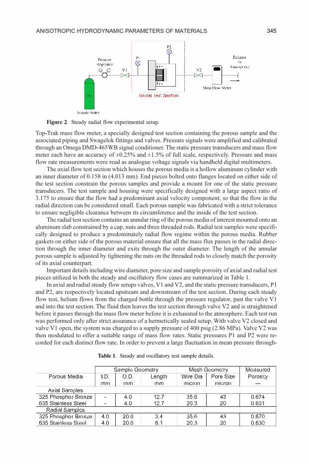
Top-Trak mass flow meter, a specially designed test section containing the porous sample and the
associated piping and Swagelok fittings and valves. Pressure signals were amplified and calibrated
through an Omega DMD-465WB signal conditioner. The static pressure transducers and mass flow
meter each have an accuracy of ±0.25% and ±1.5% of full scale, respectively. Pressure and mass
flow rate measurements were read as analogue voltage signals via handheld digital multimeters.
The axial flow test section which houses the porous media is a hollow aluminum cylinder with
an inner diameter of 0.158 in (4.013 mm). End pieces bolted onto flanges located on either side of
the test section constrain the porous samples and provide a mount for one of the static pressure
transducers. The test sample and housing were specifically designed with a large aspect ratio of
3.175 to ensure that the flow had a predominant axial velocity component; so that the flow in the
radial direction can be considered small. Each porous sample was fabricated with a strict tolerance
to ensure negligible clearance between its circumference and the inside of the test section.
The radial test section contains an annular ring of the porous media of interest mounted onto an
aluminum slab constrained by a cap, nuts and three threaded rods. Radial test samples were specifi-
cally designed to produce a predominately radial flow regime within the porous media. Rubber
gaskets on either side of the porous material ensure that all the mass flux passes in the radial direc-
tion through the inner diameter and exits through the outer diameter. The length of the annular
porous sample is adjusted by tightening the nuts on the threaded rods to closely match the porosity
of its axial counterpart.
Important details including wire diameter, pore size and sample porosity of axial and radial test
pieces utilized in both the steady and oscillatory flow cases are summarized in Table 1.
In axial and radial steady flow setups valves, V1 and V2, and the static pressure transducers, P1
and P2, are respectively located upstream and downstream of the test section. During each steady
flow test, helium flows from the charged bottle through the pressure regulator, past the valve V1
and into the test section. The fluid then leaves the test section through valve V2 and is straightened
before it passes through the mass flow meter before it is exhausted to the atmosphere. Each test run
was performed only after strict assurance of a hermetically sealed setup. With valve V2 closed and
valve V1 open, the system was charged to a supply pressure of 400 psig (2.86 MPa). Valve V2 was
then modulated to offer a suitable range of mass flow rates. Static pressures P1 and P2 were re-
corded for each distinct flow rate. In order to prevent a large fluctuation in mean pressure through-
Figure 2. Steady radial flow experimental setup.
Table 1. Steady and oscillatory test sample details.
345aniSotropic HyDroDynamic parameterS of materialS

out each sample run, a maximum allowable change in pressure across the test section was limited to
100 psi (0.69 MPa). For each test run, pressure drops between static pressures P1 and P2 were then
plotted against mass flow rate. In order to simplify the data analysis, axial – flow experimental data
for each filler material was curved fitted to a 5th order polynomial while radial test points were fitted
to a 2nd order polynomial. Each curve fit was constrained with a zero intercept and would act as a
guide for defining the boundary conditions to be used for CFD simulations.
Steady Flow Simulations and Data Analysis
Based upon the aforementioned experimental curve fit polynomials, seven representative ex-
perimental data points across the full range of mass flow rates were then input to the Fluent CFD
code, providing for the indirect solution of hydrodynamic viscous and inertial resistances. The
simulations used a two – dimensional, axisymmetric mesh that modeled the geometry of the experi-
mental test setup from stations P1 to P2. In all the simulations, helium was treated as an ideal gas
with constant viscosity. Multiple nodal networks of varying grid sizes were developed to examine
the effect of mesh size on the simulation outcomes. A mesh with the smallest number of nodes
which led to reasonable mesh size independent of results was eventually specified and applied,
affording efficient use of computational time.
A single Fluent case was created for each representative data point and experimentally-mea-
sured parameter values were input as boundary conditions for simulations. A mass flow rate bound-
ary condition was used at the inlet while a pressure outlet boundary condition was implemented
downstream at the P2 location. The model’s viscous and inertial resistances were iteratively changed
until there was agreement between the simulated area-weighted static pressure at the inlet and
experimental static pressure at P1 at all chosen data points.
Although turbulent flow was not expected in the porous section, Reynolds numbers in some
open sections were high enough to imply turbulent flow. As a result, the Reynolds–Averaged Navier
Stokes k-ε turbulence model was used in the steady axial simulations. However, conditions within
the radial test section permitted a laminar flow model in the steady radial flow simulations.
For both the axial and radial steady flow cases, the viscous resistance could be determined at low
flow rates because inertial effects were small. A trial and error method was used until a unique viscous
resistance satisfied the first several data points of the low flow regime. This term was then fixed and
only the inertial resistance was adjusted in the subsequent simulations. This method of predetermin-
ing the viscous resistance was applied to both axial and radial steady flow regimes and was modified
slightly for oscillatory cases. The iterative process was continued until good agreement was achieved
between simulated and experimental pressure drops across the entire range of mass flow rates.
Oscillatory Flow Experiments
Diagrams of the oscillatory – flow axial and radial tests setups are shown in Figures 3 and 4,
respectively. The experimental and computational procedures for determining the hydrodynamic
axial and radial flow resistances for oscillatory flow were very similar. The equipment utilized in
both cases is identical, with the exception of the porous test section, the sample housing and its
associated fittings and sensor mounts.
Figure 3. Oscillatory axial flow experimental setup.
346 regenerator moDeling anD performance inveStigationS

The oscillatory flow experimental setups consisted of a Hughes Aircraft Tactical Condor com-
pressor, HP-Agilent 33120A function waveform generator and HP-Agilent 3852A data acquisition
control unit, Crown DC-300A Series II amplifier, a constant-temperature hot wire anemometer
(HWA) with a TSI Flowpoint 1500 Series signal conditioner, two high frequency PCB Piezotronics
101A05 dynamic pressure transducers, a specially designed test section containing porous media
and the associated piping, fittings and a helium charge tank. The dynamic pressure transducers
have a resolution of 2 mpsi (0.014 kPa). Hot wire calibration curves were obtained at 2.86 MPa
(400 psig) and 500 psig (3.45 MPa) under steady flow conditions in an inline fitting using a mass
flow meter. An HP VEE virtual console was operated to integrate all sensor measurements and store
their output data. An iron core transformer was also utilized to offer better power transmission from
the amplifier to the compressor.
The experimental setup for periodic flow is a closed system bounded by the compressor and
the valve, V1. Both the axial and radial oscillatory flow test sections consist of the same sample
pieces and housing utilized in their steady flow counterparts. Dynamic pressure transducer P1 and
hot wire probe HW1 are located on the compressor side of the test section while dynamic pressure
transducer P2 is positioned on the opposite side of the test section.
For the axial case, pressure sensors and HWA are mounted onto end pieces adjoining the sample
housing while in the radial test setup the transducers are installed via inline fittings. Axial sensor
mounts on either side of the cylindrical housing are also internally fitted with an 8.0° sloped transi-
tion cone located between the porous media and sensor tap locations. This transition is meant to
avoid a large step change in pipe diameter and acts to reduce flow disturbance, resulting in an
unwavering hot wire signal.
A sinusoidal signal sent to the compressor is amplified to provide the largest stable pressure
oscillation at each discrete frequency. Waveforms from the hotwires are directly recorded to com-
pare with the Fluent model results, while the periodic pressures are represented by their first three
harmonics, calculated using a fast Fourier transform (FFT) following the method described by
Cha.1,3 Data was taken at seven distinct frequencies in the 50 to 200 Hz range, in intervals of 25 Hz,
at operating pressures of approximately 2.86 MPa and 3.55 MPa (400 and 500 psig). High charge
pressures and high operating frequencies were selected because they are expected to apply to min-
iature cryocoolers.
Oscillatory Flow Simulations and Data Analysis
The experimental test section geometry between pressure transducer P1 and valve V1 is mod-
eled by a two-dimensional axisymmetric mesh, and is simulated using the Fluent CFD code assum-
ing laminar flow regime. A user defined oscillatory pressure inlet boundary condition is applied at
P1 based upon the aforementioned Fourier series representation of the experimental measurements.
Like its steady state counterpart, the viscous resistance was initially determined at 50 Hz low flow
conditions, where inertial effects were considered small. Once a range of prescribed viscous resis-
tances were established, inertial resistances were added.
The iterative determination of the viscous and inertial resistances was similar to the aforemen-
tioned steady flow tests. Accordingly, the viscous resistance term was first quantified using experi-
Figure 4. Oscillatory radial flow experimental setup.
347aniSotropic HyDroDynamic parameterS of materialS

mental data with low flow conditions. Subsequently, the viscous resistance coefficient was kept
constant while the inertial resistance term was iteratively adjusted until agreement was achieved
between the simulated area-weighted static pressure at P2 and experimentally measured static pres-
sure at that location. The periodic flow axial hydrodynamic parameters were further validated by
comparing experimental velocity data from HW1 to simulated centerline velocity magnitudes at
the same location. This data, however, is not presented in this paper.
RESULTS
The volume-averaged momentum conservation equation for flow through a porous medium
can be written5 as:
(1)
This equation, along with mass and energy conservation equations are numerically solved by
the CFD code. The sample porosity is represented by ε while the viscous and inertial resistance
coefficient tensors are D� and C
� with units of 1/m2 and 1/m, respectfully. Fluid density and viscos-
ity are displayed as ρ and μ, and τ� represents the stress tensor. Thermodynamic pressure is shown
with P and F→
bf represents the body force vectors (our particular simulations do not include any
body forces or gravity). The vector u→ represents the physical velocity within the porous structure.
Assuming isotropic flow resistances, the viscous and inertial resistance coefficients will be scalar
quantities. The last two terms in the above equation, which together represent the total resistance
force, can then be used for the definition of the Darcy permeability and Forchheimer’s inertial
coefficient according to:
(2)
(3)
(4)
For steady and oscillatory flow hydrodynamic parameter determination, isotropic viscous and
inertial resistances were assumed in Fluent simulations. This simplifying assumption was justified
because the flow within the porous structure of each test apparatus was predominantly one-dimen-
sional.
Steady Flow Parameters
Fluent simulations6 were performed for both porous structures at a supply pressure of 2.86 MPa
(400 psig). Figures 5 and 6 display pressure drop as a function of mass flow rate for the two axial
Figure 5. Steady axial flow pressure plot.
348 regenerator moDeling anD performance inveStigationS
and radial flow test sections, respectively. Curves representing the simulation results are also shown
along with the discrete experimental data points for comparison.
Multiple test runs were performed for each mesh filler producing mass flow rates ranging from
0.042 g/s to 1.36 g/s. The pressure drop was limited to 6.9 bar (100 psi) in each test, however. The
axial steady – flow measurements were found to be well repeatable. Due to the small cross sectional
area of the axial test sample and housing, large pressure drops of up to 674 kPa were recorded in
those tests. As noted in Figure 5, good agreement is displayed between steady axial experimental
and simulated data over the entire range of flow rates.
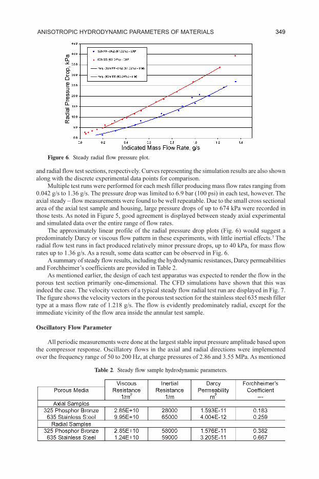
The approximately linear profile of the radial pressure drop plots (Fig. 6) would suggest a
predominately Darcy or viscous flow pattern in these experiments, with little inertial effects.7 The
radial flow test runs in fact produced relatively minor pressure drops, up to 40 kPa, for mass flow
rates up to 1.36 g/s. As a result, some data scatter can be observed in Fig. 6.
A summary of steady flow results, including the hydrodynamic resistances, Darcy permeabilities
and Forchheimer’s coefficients are provided in Table 2.
As mentioned earlier, the design of each test apparatus was expected to render the flow in the
porous test section primarily one-dimensional. The CFD simulations have shown that this was
indeed the case. The velocity vectors of a typical steady flow radial test run are displayed in Fig. 7.
The figure shows the velocity vectors in the porous test section for the stainless steel 635 mesh filler
type at a mass flow rate of 1.218 g/s. The flow is evidently predominately radial, except for the
immediate vicinity of the flow area inside the annular test sample.
Oscillatory Flow Parameter
All periodic measurements were done at the largest stable input pressure amplitude based upon
the compressor response. Oscillatory flows in the axial and radial directions were implemented
over the frequency range of 50 to 200 Hz, at charge pressures of 2.86 and 3.55 MPa. As mentioned
Figure 6. Steady radial flow pressure plot.
Table 2. Steady flow sample hydrodynamic parameters.
349aniSotropic HyDroDynamic parameterS of materialS
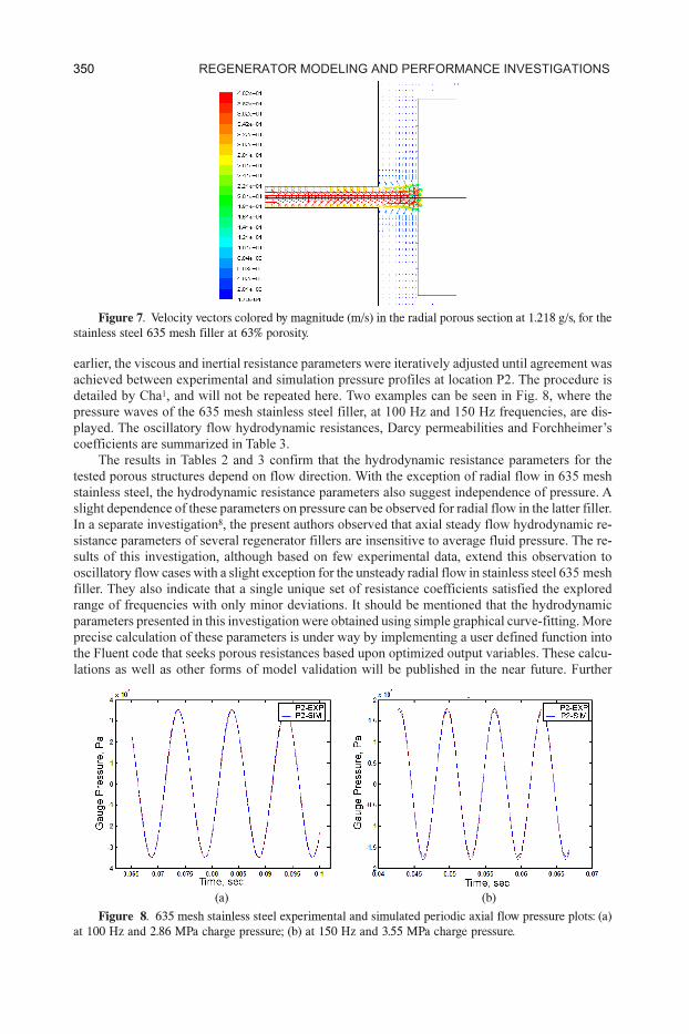
Figure 7. Velocity vectors colored by magnitude (m/s) in the radial porous section at 1.218 g/s, for the
stainless steel 635 mesh filler at 63% porosity.
earlier, the viscous and inertial resistance parameters were iteratively adjusted until agreement was
achieved between experimental and simulation pressure profiles at location P2. The procedure is
detailed by Cha1, and will not be repeated here. Two examples can be seen in Fig. 8, where the
pressure waves of the 635 mesh stainless steel filler, at 100 Hz and 150 Hz frequencies, are dis-
played. The oscillatory flow hydrodynamic resistances, Darcy permeabilities and Forchheimer’s
coefficients are summarized in Table 3.
The results in Tables 2 and 3 confirm that the hydrodynamic resistance parameters for the
tested porous structures depend on flow direction. With the exception of radial flow in 635 mesh
stainless steel, the hydrodynamic resistance parameters also suggest independence of pressure. A
slight dependence of these parameters on pressure can be observed for radial flow in the latter filler.
In a separate investigation8, the present authors observed that axial steady flow hydrodynamic re-
sistance parameters of several regenerator fillers are insensitive to average fluid pressure. The re-
sults of this investigation, although based on few experimental data, extend this observation to
oscillatory flow cases with a slight exception for the unsteady radial flow in stainless steel 635 mesh
filler. They also indicate that a single unique set of resistance coefficients satisfied the explored
range of frequencies with only minor deviations. It should be mentioned that the hydrodynamic
parameters presented in this investigation were obtained using simple graphical curve-fitting. More
precise calculation of these parameters is under way by implementing a user defined function into
the Fluent code that seeks porous resistances based upon optimized output variables. These calcu-
lations as well as other forms of model validation will be published in the near future. Further
Figure 8. 635 mesh stainless steel experimental and simulated periodic axial flow pressure plots: (a)
at 100 Hz and 2.86 MPa charge pressure; (b) at 150 Hz and 3.55 MPa charge pressure.
(a) (b)
350 regenerator moDeling anD performance inveStigationS
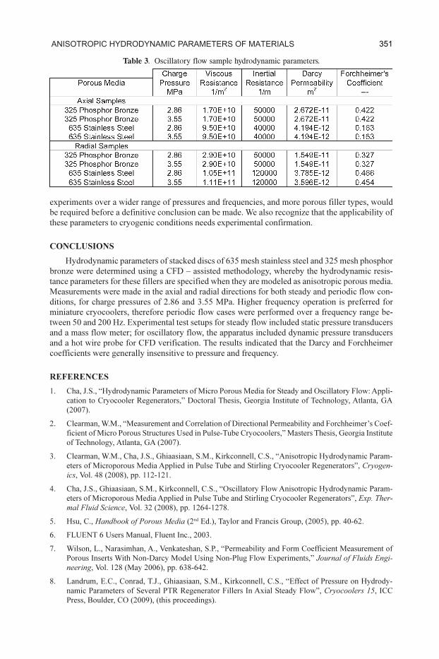
Table 3. Oscillatory flow sample hydrodynamic parameters.
experiments over a wider range of pressures and frequencies, and more porous filler types, would
be required before a definitive conclusion can be made. We also recognize that the applicability of
these parameters to cryogenic conditions needs experimental confirmation.
CONCLUSIONS
Hydrodynamic parameters of stacked discs of 635 mesh stainless steel and 325 mesh phosphor
bronze were determined using a CFD – assisted methodology, whereby the hydrodynamic resis-
tance parameters for these fillers are specified when they are modeled as anisotropic porous media.
Measurements were made in the axial and radial directions for both steady and periodic flow con-
ditions, for charge pressures of 2.86 and 3.55 MPa. Higher frequency operation is preferred for
miniature cryocoolers, therefore periodic flow cases were performed over a frequency range be-
tween 50 and 200 Hz. Experimental test setups for steady flow included static pressure transducers
and a mass flow meter; for oscillatory flow, the apparatus included dynamic pressure transducers
and a hot wire probe for CFD verification. The results indicated that the Darcy and Forchheimer
coefficients were generally insensitive to pressure and frequency.
REFERENCES
1. Cha, J.S., “Hydrodynamic Parameters of Micro Porous Media for Steady and Oscillatory Flow: Appli-
cation to Cryocooler Regenerators,” Doctoral Thesis, Georgia Institute of Technology, Atlanta, GA
(2007).
2. Clearman, W.M., “Measurement and Correlation of Directional Permeability and Forchheimer’s Coef-
ficient of Micro Porous Structures Used in Pulse-Tube Cryocoolers,” Masters Thesis, Georgia Institute
of Technology, Atlanta, GA (2007).
3. Clearman, W.M., Cha, J.S., Ghiaasiaan, S.M., Kirkconnell, C.S., “Anisotropic Hydrodynamic Param-
eters of Microporous Media Applied in Pulse Tube and Stirling Cryocooler Regenerators”, Cryogen-
ics, Vol. 48 (2008), pp. 112-121.
4. Cha, J.S., Ghiaasiaan, S.M., Kirkconnell, C.S., “Oscillatory Flow Anisotropic Hydrodynamic Param-
eters of Microporous Media Applied in Pulse Tube and Stirling Cryocooler Regenerators”, Exp. Ther-
mal Fluid Science, Vol. 32 (2008), pp. 1264-1278.
5. Hsu, C., Handbook of Porous Media (2nd Ed.), Taylor and Francis Group, (2005), pp. 40-62.
6. FLUENT 6 Users Manual, Fluent Inc., 2003.
7. Wilson, L., Narasimhan, A., Venkateshan, S.P., “Permeability and Form Coefficient Measurement of
Porous Inserts With Non-Darcy Model Using Non-Plug Flow Experiments,” Journal of Fluids Engi-
neering, Vol. 128 (May 2006), pp. 638-642.
8. Landrum, E.C., Conrad, T.J., Ghiaasiaan, S.M., Kirkconnell, C.S., “Effect of Pressure on Hydrody-
namic Parameters of Several PTR Regenerator Fillers In Axial Steady Flow”, Cryocoolers 15, ICC
Press, Boulder, CO (2009), (this proceedings).
351aniSotropic HyDroDynamic parameterS of materialS