Rao Electromagnetics for Fundamentals of Electromagnetics for
Progress In Electromagnetics Research B, Vol. 2, 27–60, 2008
AN INTRODUCTION TO SYNTHETIC APERTURERADAR (SAR)
Y. K. Chan and V. C. Koo
Faculty of Engineering & TechnologyMultimedia UniversityJalan Ayer Keroh Lama, Bukit Beruang, 75450 Melaka, Malaysia
Abstract—This paper outlines basic principle of Synthetic ApertureRadar (SAR). Matched filter approaches for processing the receiveddata and pulse compression technique are presented. Besides the SARradar equation, the linear frequency modulation (LFM) waveform andmatched filter response are also discussed. Finally the system designconsideration of various parameters and aspects are also highlighted.
1. INTRODUCTION
Radar has long been used for military and non-military purposes in awide variety of applications such as imaging, guidance, remote sensingand global positioning [1]. Development of radar as a tool for shipand aircraft detection was started during 1920s. In 1922, the firstcontinuous wave radar system was demonstrated by Taylor. The firstpulse radar system was developed in 1934 with operating frequency60 MHz by Naval Research Laboratory (NRL), US. At the same time,radar systems for tracking and detection of aircraft were developedboth in Great Britain and Germany during the early 1930s.
The first imaging radar, developed during World War II, usedthe B-Scan which produced an image in a rectangular format. Thenonlinear relation between angle and distance to the side of aircraftproduced great distortions on the display. This distortion was greatlyimproved by development of Plan Position Indicator (PPI). Its antennabeam was rotated through 360◦ about the aircraft and a picture ofground was produced. In the 1950s, the Side Looking Airborne Radar(SLAR) was developed. Scanning had been achieved with the SLAR byfixed beam pointed to the side with aircraft’s motion moving the beamacross the land. The early versions of SLAR systems were primarilyused for military reconnaissance purposes. Until mid 1960s, the first

28 Chan and Koo
high-resolution SLAR image was declassified and made available forscientific use.
However, the image formed by SLAR is poor in azimuth resolution.For SLAR the smaller the azimuth beamwidth, the finer the azimuthresolution. In order to obtain high-resolution image one has to resorteither to an impractically long antenna or to employ wavelengths soshort that the radar must contend with severe attenuation in theatmosphere. In airborne application particularly the antenna sizeand weight are restricted. Another way of achieving better resolutionfrom radar is signal processing. Synthetic Aperture Radar (SAR) isa technique which uses signal processing to improve the resolutionbeyond the limitation of physical antenna aperture [2]. In SAR,forward motion of actual antenna is used to ‘synthesize’ a very longantenna. SAR allows the possibility of using longer wavelengths andstill achieving good resolution with antenna structures of reasonablesize.
In 1952, “Doppler beam-sharpening” system was developed byWiley of Goodyear Corporation. This system was not side lookingradar. It operated in squint mode with the beam point around 45◦ahead. The radar group at Goodyear research facility in Litchfield,Arizona pursued Wiley’s concept and built the first airborne SARsystem, flown aboard a DC-3 in 1953. The radar system operatedat 930 MHz, used a Yagi antenna with real aperture beamwidth of100◦. During the late 1950s, and early 1960s, classified developmentof SAR systems took place at the University of Michigan and at somecompanies. At the same time, similar developments were conductingin other country such as Russia, France and United Kingdom.
The use of SAR for remote sensing is particularly suited fortropical countries. By proper selection of operating frequency, themicrowave signal can penetrate clouds, haze, rain and fog andprecipitation with very little attenuation, thus allowing operationin unfavourable weather conditions that preclude the use ofvisible/infrared system [3]. Since SAR is an active sensor, whichprovides its own source of illumination, it can therefore operateday or night; able to illuminate with variable look angle and canselect wide area coverage. In addition, the topography change canbe derived from phase difference between measurement using radarinterferomentry. SAR has been shown to be very useful over a widerange of applications, including sea and ice monitoring [4], mining [5],oil pollution monitoring [6], oceanography [7], snow monitoring [8],classification of earth terrain [9] etc. The potential of SAR in a diverserange of application led to the development of a number of airborneand spaceborne SAR systems.

Progress In Electromagnetics Research B, Vol. 2, 2008 29
Some SAR systems are described as follow. A polarimetricairborne SAR system was developed by NASA Jet PropulsionLaboratory (JPL) and loaded on CV-990 aircraft system [10]. Theradar was operated at a wavelength of 24.5 cm (L-band) and hada 4-look resolution of about 10 m by 10 m. In July 1985, the CV-990 together with the SAR instrumentation was destroyed by fireduring an aborted takeoff from March Air Force Base in SouthernCalifornia. After the disaster, a new imaging radar (AIRSAR) wasbuilt at JPL and this system incorporates all the characteristics ofthe previous CV-990 L-band SAR. Fig. 1.1 shows the basic blockdiagram of the CV-990 system. The CV-990 system employed twoseparate antennas, one horizontally polarised and the other verticallypolarised. Full polarisation can be achieved by transmits a pulses trainthrough the switching circuitry. The pulses are transmitted throughhorizontal polarised antenna and received signal from both antenna.Then followed by transmits vertical polarised pulse and received byboth antenna. Circulators permit a single antenna to be used forboth transmission and reception. The CV-990 radar has served asthe prototype for all other currently operating imaging radar and forthe spaceborne system proposed by NASA for operation in 1990s.
PulseTransmitter
Switch
HorizontalAntenna
HorizontalReceiver
VerticalAntennaVertical
ReceiverCirculator
CirculatorAmplifier
Amplifier
Figure 1.1. Basic block diagram of the CV-990 polarimetric SARsystem.
The AIRSAR system was built based on CV-990 L-band SAR andextended to include P-Band (440 MHz) and C-band (5300 MHz) [11].The new system is capable of producing fully polarimetric data from allthree frequencies simultaneously. It collects HH, HV, VH and VV dataat all three frequencies with approximately 10 m resolution. Fig. 1.2shows the functional diagram of AIRSAR. The system has a singlestable local oscillator (STALO) clock and a single exciter source, whichoperates at L-Band. Each generated chirp is up-converted to C-Bandand down-converted to P-Band. Each of the P- and L-Band signal is

30 Chan and Koo
amplified by a travelling wave tube (TWT). For C-Band, 2 TWTs areused before the signal is split into H and V channels for transmission.The H and V transmission events are separated in time by half a pulserepetition interval. The TWTs give peak power outputs of 6 kW at L-Band and 1 kW at P- and C-Band. A wide dynamic range is achievedby using 8-bit analogue-to-digital converters (ADC’s). The ADC’s eachoperates at 45 MHz and produces real-data samples (not I and Q) ata total data rate of between 20 and 60 Mbytes/second. The data fromeach receiver channel is multiplexed together for recording onto any ofthe three available HDDRs.
Buffer
Annotator
Formatter
HDDRFormatter
HDDR
Antenna Control
FWD AFTH V H V
RCVR
XMTR
RCVR
UPCON
ADC
ADCCalibration
C
Antenna Control
FWD AFTH V H V
RCVR
XMTR
RCVR
EXCITER
ADC
ADC
Calibration
L STALO
Antenna Control
AFTH V
RCVR
XMTR
RCVR
DWNCON
ADC
ADC
Calibration
PUHF
10 Mbytes/sec
EngineeringData Inputs
AFT: Aft Antenna (Aft Data)FWD: Fore Antenna (Forward Data)RCVR: ReceiverXMTR: TransmitterUPCON: Up-converterDWNCON: Down-converter
Figure 1.2. NASA/JPL aircraft imaging radar functional diagram.
One of the inexpensive SAR system is the Brigham YoungUniversity SAR (YSAR) [12]. Typical SAR system is complex,expensive and difficult to transport but the YSAR is relativelyinexpensive and lightweight. This system is to be flown in four orsix passenger aircraft at altitudes up to 2000 feet. The simplifiedblock diagram of YSAR is shown in Fig. 1.3. The baseband chirpis generated by a low-cost 200 MHz Arbitrary Waveform Generator(AWG). The transmitter mixes the 100 MHz bandwidth chirp up to2.1 GHz for transmission. The chirp is transmitted and received withdouble-sideband (DSB) modulation to reduce the cost. The receiverand local oscillator are used to mix the RF radar return from theantenna to an offset baseband and amplify it so it can be sampled
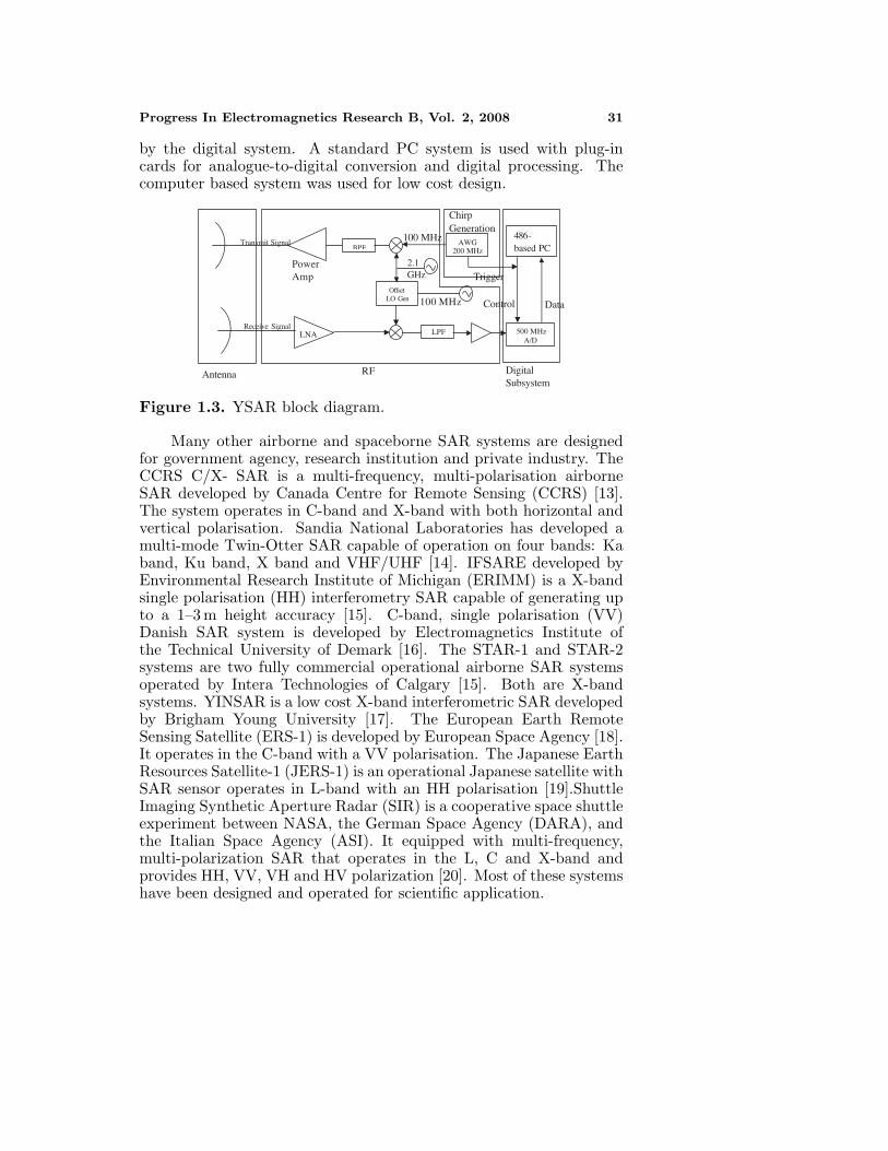
Progress In Electromagnetics Research B, Vol. 2, 2008 31
by the digital system. A standard PC system is used with plug-incards for analogue-to-digital conversion and digital processing. Thecomputer based system was used for low cost design.
AWG200 MHzBPF
OffsetLO Gen
LPF
486-based PC
500 MHz A/D
PowerAmp
Transmit Signal
LNAReceive Signal
ChirpGeneration
100 MHz
Trigger
Control Data100 MHz
DigitalSubsystem
RFAntenna
2.1GHz
Figure 1.3. YSAR block diagram.
Many other airborne and spaceborne SAR systems are designedfor government agency, research institution and private industry. TheCCRS C/X- SAR is a multi-frequency, multi-polarisation airborneSAR developed by Canada Centre for Remote Sensing (CCRS) [13].The system operates in C-band and X-band with both horizontal andvertical polarisation. Sandia National Laboratories has developed amulti-mode Twin-Otter SAR capable of operation on four bands: Kaband, Ku band, X band and VHF/UHF [14]. IFSARE developed byEnvironmental Research Institute of Michigan (ERIMM) is a X-bandsingle polarisation (HH) interferometry SAR capable of generating upto a 1–3 m height accuracy [15]. C-band, single polarisation (VV)Danish SAR system is developed by Electromagnetics Institute ofthe Technical University of Demark [16]. The STAR-1 and STAR-2systems are two fully commercial operational airborne SAR systemsoperated by Intera Technologies of Calgary [15]. Both are X-bandsystems. YINSAR is a low cost X-band interferometric SAR developedby Brigham Young University [17]. The European Earth RemoteSensing Satellite (ERS-1) is developed by European Space Agency [18].It operates in the C-band with a VV polarisation. The Japanese EarthResources Satellite-1 (JERS-1) is an operational Japanese satellite withSAR sensor operates in L-band with an HH polarisation [19].ShuttleImaging Synthetic Aperture Radar (SIR) is a cooperative space shuttleexperiment between NASA, the German Space Agency (DARA), andthe Italian Space Agency (ASI). It equipped with multi-frequency,multi-polarization SAR that operates in the L, C and X-band andprovides HH, VV, VH and HV polarization [20]. Most of these systemshave been designed and operated for scientific application.

32 Chan and Koo
2. PRINCIPLE OF SAR
2.1. Introduction
RADAR is an acronym for RAdio Detection And Ranging. Radarworks like a flash camera but at radio frequency. Typical radar systemconsists of transmitter, switch, antenna, receiver and data recorder.The transmitter generates a high power of electromagnetic wave atradio wavelengths. The switch directed the pulse to antenna andreturned echo to receiver. The antenna transmitted the EM pulsetowards the area to be imaged and collects returned echoes. Thereturned signal is converted to digital number by the receiver and thefunction of the data recorder is to store data values for later processingand display. Fig. 2.1 shows the simply block diagram of a radar system.
Transmitter
Receiver
Switch
Data Recorder Processor Display
AntennaRadar pulse
Figure 2.1. Basic block diagram of typical radar system.
The radar platform flies along the track direction at constantvelocity. For real array imaging radar, its long antenna produces afan beam illuminating the ground below. The along track resolution isdetermined by the beamwidth while the across resolution is determinedby the pulse length. The larger the antenna, the finer the detail theradar can resolve.
In SAR, forward motion of actual antenna is used to ‘synthesize’ avery long antenna. At each position a pulse is transmitted, the returnechoes pass through the receiver and recorded in an ‘echo store’. TheDoppler frequency variation for each point on the ground is uniquesignature. SAR processing involves matching the Doppler frequencyvariations and demodulating by adjusting the frequency variation inthe return echoes from each point on the ground. Result of thismatched filter is a high-resolution image. Figure below shows thesynthetic aperture length.

Progress In Electromagnetics Research B, Vol. 2, 2008 33
TransmitterReceiver
Echo store
TransmitterReceiver
Echo store
TransmitterReceiver
Echo store
Direction of platform motion
Synthetic Aperture Length, L
Figure 2.2. Synthetic aperture.
2.2. The Description of an Imaging Radar
The geometry of an imaging radar is shown in Fig. 2.3. The physicalaperture of the radar with width Wa and length � generates a RF beamwhose angular across track 3 dB beamwidth of antenna and angularalong-track 3 dB beamwidth of antenna is θV and θH respectively. θV
is determined by the width and length of antenna, and wavelength oftransmitted signal (λ). This relation is written as [2],
θV = λ/Wa (2.1)
The antenna is mounted on a platform such as an aircraft thattravels along a flight path with velocity v. It illuminates the shadedpath (known as footprint) on the ground as the aircraft moves in thedirection of flight path. The width of the ground swath is simply givenby
Wg =λR
Wa cos θ(2.2)
where θ is the incidence angle (look angle) of the beam, R is the slantrange from the antenna to the midpoint of swath.
The RF energy transmitted from antenna has a duration τp andis repeated at a given interval, pulse repetition interval (PRI) that canbe inverted to obtain the pulse repetition frequency (PRF).
2.2.1. The Resolution of a Real Aperture Radar
Ground resolution is defined as the ability of the system to distinguishbetween two targets on the ground. Ground range resolution is shown

34 Chan and Koo
vTrajectory
Wa
SAR Antenna
Look angle, θ
τ p
Radiated Pulse
θV
θH
Wg
SwathFootprint
l
Figure 2.3. The imaging radar geometry.
in Fig. 2.4 as ρg. The range resolution of real aperture radar is givenas [2],
ρg =cτp
2 sin θ(2.3)
where τp is the pulse length and c is the speed of light. The rangeresolution is the function of pulse width and look angle but independentof height.
Azimuth resolution is the minimum distance on the ground in thedirection parallel to the flight path of the aircraft at which two targetscan be separately imaged. Two targets located at same slant range canbe resolved only if they are not in the radar beam at the same time.Fig. 2.5 shows the angular spread of the radar beam in the azimuthdirection is equal to
θH = λ/� (2.4)

Progress In Electromagnetics Research B, Vol. 2, 2008 35
ctRo
θ V
θ
Wg
ρg
Figure 2.4. Range resolution of a real aperture radar.
Thus, the azimuth resolution can be written as,
ρa = RθH =Rλ
�(2.5)
The azimuth resolution is dependent on aperture length. Inorder to improve resolution, a longer antenna needs to be employed.The mechanical problems involved in constructing an antenna witha surface precision accurate to within a fraction of wavelength, andthe difficulty in maintaining that level of precision in an operationalenvironment, make it difficult to attain values of �/λ greater than afew hundred aperture [2].
2.2.2. Resolution of Synthetic Aperture Radar
SAR is based on the generation of an effective long antenna by signalprocessing means rather than by the actual use of a long physicalantenna. The SAR processing can be achieved by utilising the Dopplereffect (frequency shift) of the echo signal [21].
The geometry of SAR is shown in Fig. 2.6. The aircraft is mappingthe point, p, whose coordinates are xo, yo, 0. The aircraft will fly asynthetic array of length L, centered at y = 0 at speed v, parallel tothe y-axis and altitude, ho. The time to fly the array is T = L/v. Therange from the aircraft to p can be written
R =√x2
o + (yo − vt)2 + h2o (2.6)
where −T/2 ≤ t ≤ T/2, for L � R, Ro =√x2
o + y2o + h2
o and
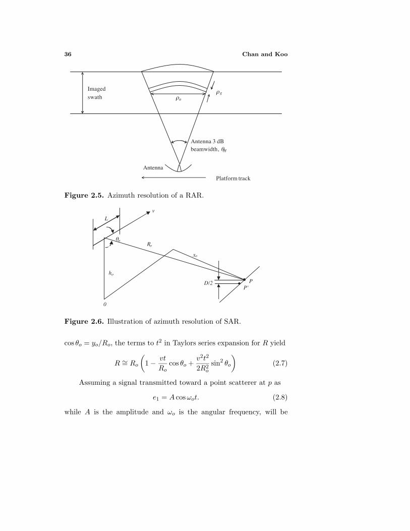
36 Chan and Koo
Imagedswath
Platform track
Antenna
Antenna 3 dB beamwidth, θH
ρ gρa
Figure 2.5. Azimuth resolution of a RAR.
v
L
Ro
ho
0
D/2 PP'
xo
θo
Figure 2.6. Illustration of azimuth resolution of SAR.
cos θo = yo/Ro, the terms to t2 in Taylors series expansion for R yield
R ∼= Ro
(1 − vt
Rocos θo +
v2t2
2R2o
sin2 θo
)(2.7)
Assuming a signal transmitted toward a point scatterer at p as
e1 = A cosωot. (2.8)
while A is the amplitude and ωo is the angular frequency, will be

Progress In Electromagnetics Research B, Vol. 2, 2008 37
reflected and received at the aircraft with a time delay τ ′ so that
e2 = KA cosωo(t− τ ′) (2.9)
where K is a constant and e2 is the received signal. The time delayis given as a function of range, R, as τ ′ = 2R/c. Thus, time delaybecomes,
τ ′ =2Ro
c− 2vt
ccos θo +
v2t2
Rocsin2 θo (2.10)
The argument of the received signal with this substitution for τ ′ is
θ(t) = ωo(t− τ ′)
= ωot−2ωoRo
c+
2ωovt
ccos θo −
ωov2t2
Rocsin2 θo (2.11)
In terms of wavelength, λ = 2πc/ωo,
θ(t) = ωot−4πRo
λ+
4πλvt cos θo −
2πv2t2
Roλsin2 θo (2.12)
Using the usual definition of the instantaneous frequency as
fi =12π
dθ(t)dt
(2.13)
thus, we get
fi = fo +2vλ
cos θo −2v2t
Roλsin2 θo (2.14)
where fo = ωo/2π. The second term is the doppler shift associatedwith the squint angle θo. The third term represents the change indoppler shift due to the forward motion of the aircraft.
The instantaneous frequency for the two targets, p and p′, bothat a distance of Ro but separated in azimuth by a distance, D/2, willbe
fo +2vλ
cos θo and fo +2vλ
cos θo −vD
Roλsin θo
since the time to fly the distance between them is t = D sin θo/2v andthe observed differential frequency shift ∆fi will be
∆fi =vD
Roλsin θo (2.15)
38 Chan and Koo
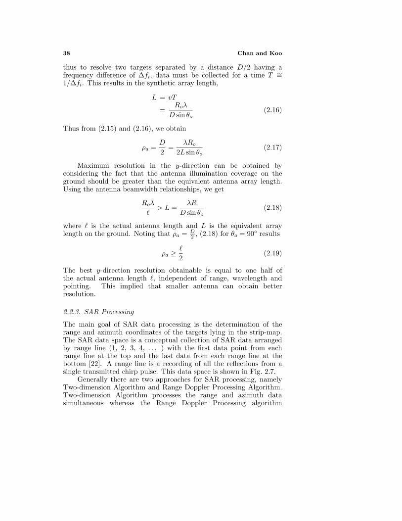
thus to resolve two targets separated by a distance D/2 having afrequency difference of ∆fi, data must be collected for a time T ∼=1/∆fi. This results in the synthetic array length,
L = vT
=Roλ
D sin θo(2.16)
Thus from (2.15) and (2.16), we obtain
ρa =D
2=
λRo
2L sin θo(2.17)
Maximum resolution in the y-direction can be obtained byconsidering the fact that the antenna illumination coverage on theground should be greater than the equivalent antenna array length.Using the antenna beamwidth relationships, we get
Roλ
�> L =
λR
D sin θo(2.18)
where � is the actual antenna length and L is the equivalent arraylength on the ground. Noting that ρa = D
2 , (2.18) for θo = 90◦ results
ρa ≥ �
2(2.19)
The best y-direction resolution obtainable is equal to one half ofthe actual antenna length �, independent of range, wavelength andpointing. This implied that smaller antenna can obtain betterresolution.
2.2.3. SAR Processing
The main goal of SAR data processing is the determination of therange and azimuth coordinates of the targets lying in the strip-map.The SAR data space is a conceptual collection of SAR data arrangedby range line (1, 2, 3, 4, . . . ) with the first data point from eachrange line at the top and the last data from each range line at thebottom [22]. A range line is a recording of all the reflections from asingle transmitted chirp pulse. This data space is shown in Fig. 2.7.
Generally there are two approaches for SAR processing, namelyTwo-dimension Algorithm and Range Doppler Processing Algorithm.Two-dimension Algorithm processes the range and azimuth datasimultaneous whereas the Range Doppler Processing algorithm
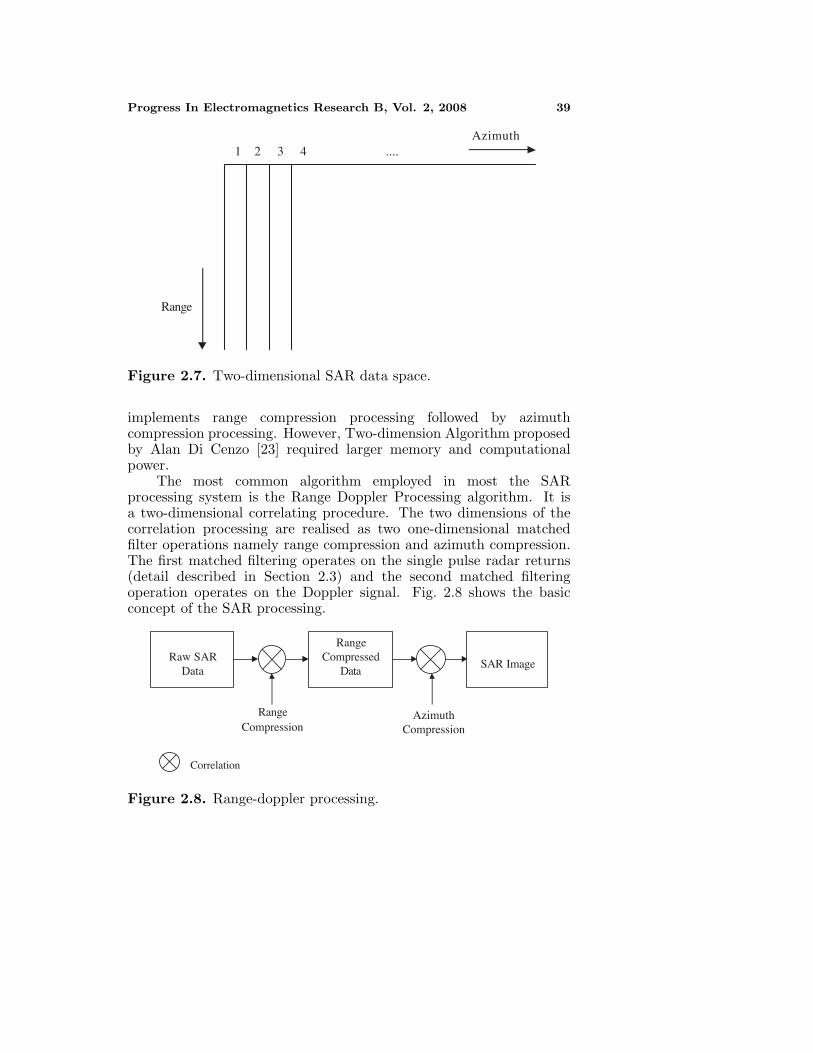
Progress In Electromagnetics Research B, Vol. 2, 2008 39
1 2 3 4 ....Azimuth
Range
Figure 2.7. Two-dimensional SAR data space.
implements range compression processing followed by azimuthcompression processing. However, Two-dimension Algorithm proposedby Alan Di Cenzo [23] required larger memory and computationalpower.
The most common algorithm employed in most the SARprocessing system is the Range Doppler Processing algorithm. It isa two-dimensional correlating procedure. The two dimensions of thecorrelation processing are realised as two one-dimensional matchedfilter operations namely range compression and azimuth compression.The first matched filtering operates on the single pulse radar returns(detail described in Section 2.3) and the second matched filteringoperation operates on the Doppler signal. Fig. 2.8 shows the basicconcept of the SAR processing.
Raw SAR Data
RangeCompressed
DataSAR Image
RangeCompression
AzimuthCompression
Correlation
Figure 2.8. Range-doppler processing.

40 Chan and Koo
2.3. Matched Filter and Pulse Compression
The matched filter and pulse compression concepts are the basic of SARprocessing algorithms [2]. The matched filter is a filter whose impulseresponse, or transfer function is determined by a certain signal, in a waythat will result in the maximum attainable signal to noise ratio. Pulsecompression involves using a matched filter to compress the energy ina signal into a relative narrow pulse.
2.3.1. Basic Properties of Matched Filter
A matched filter is designed to maximise the response of a linear systemto particular known signal. Fig. 2.9 shows the basic block diagram ofa matched filter radar system. The transmitted waveform is generatedby a signal generator designated as s(t). The signal output from s(t) isamplified, fed to antenna, radiated, reflected from a target and returnto receiver. The output of receiver is fed into the matched filter aftersuitable amplification. The matched filter impulse response, h(t), issimply a scaled, time reversed and delayed form of the input signal.The shape of the impulse response is related to the signal and thereforematched to the input. The matched filter has the property of beingable to detect the signal even in the presence of noise. It yields a higheroutput peak signal to mean noise power ratio for the input than forany other signal shape with the same energy content.
s(t) Transmittersection
Receiversection
TR
h(t)Matched filter
Antenna
Figure 2.9. Basic matched filter radar system.
Assuming return signal is a replica of transmitted signal with atime delay to. The filter is matched to s(t) and has an impulse responseof
h(t) = Ks(to − t) (2.20)
where to is a delay and K is a constant. The Fourier Transform (FT)of the impulse response of h(t) is known as the transfer function of the

Progress In Electromagnetics Research B, Vol. 2, 2008 41
matched filter, H(jw) and can be written as
H(jw) = FT{h(t)} (2.21)
H(jw) =∫ ∞
−∞h(t)e−jwtdt (2.21)
Substituting h(t) from Equation (2.20),
H(jw) = K
∫ ∞
−∞s(to − t)e−jwtdt (2.23)
By changing the time variable as, τ = to − t, (2.23) is given as,
H(jw) = −K∫ ∞
−∞s(τ)ejwτdτ (2.24)
The FT of s(t) is written as,
S(jw) =∫ ∞
−∞s(τ)e−jwtdt (2.25)
The complex conjugate of S(jw), S∗(jw) is given as
S∗(jw) = S(−jw) (2.26)
From the equations above, H(jw) can be written as,
H(jw) = −Ke−jwtoS∗(jw) (2.27)
The transfer function of the matched filter obtained is the complexconjugate of the spectrum of the signal to which it is matched. Hence,the impulse response h(t) of the matched filter is a scaled, time reversedand delayed version of the desired signal.
The output of a matched filter when a signal, s(t) is impressedat the input can be computed with the expressions derived for thetransfer function. In the time domain, the output can be obtainedeither by the convolution integral or the cross correlation integral. Forthe convolution integral, let y(t) be the output of the matched filter.The output, y(t), is then given by:
y(t) = h(t) ∗ s(t) =∫ ∞
−∞h(t− u)s(u)du (2.28)

42 Chan and Koo
Since the input signal lasts for a short duration, the output is givenby:
y(t) =∫ τ/2
−τ/2h(t− u)s(u)du (2.29)
If the cross correlation integral is considered, the output is given bythe cross correlation of h(−t) ⊗ s(t) as:
y(t) = h(−t) ⊗ s(t) =∫ τ/2
−τ/2h(−u)s(t+ u)du (2.30)
Changing the time variable as −u = t− v, (2.30) is given as
y(t) = h(−t) ⊗ s(t) =∫ t+τ/2
t−τ/2h(t− v)s(v)dv (2.31)
or,
y(t) = h(−t) ⊗ s(t) =∫ τ/2
−τ/2h(t− v)s(v)dv (2.32)
Equations (2.29) and (2.32) are essentially equivalent, exceptfor the sign reversal in the impulse response function for the crosscorrelation integral. Thus y(t) is,
y(t) = h(t) ∗ s(t) = h(−t) ⊗ s(t) =∫ τ/2
−τ/2h(t)s(τ − t)dt (2.33)
In the frequency domain, the output, Y (jw) can be obtained from thetransfer function as follows:
Y (jw) = H(jw)S(jw) = −Ke−jwtoS(jw)S∗(jw) (2.34)
The output, y(t), is obtained by taking the Inverse Fourier Transform(IFT) as shown below,
y(t) = IFT{Y (jw)} (2.35)
2.3.2. Pulse Compression
Range resolution for a given radar can be significantly improvedby using short pulse. Unfortunately utilising short pulse decreasesthe average power, which degrades radar signal detectability and

Progress In Electromagnetics Research B, Vol. 2, 2008 43
measurement precision. Since the average transmitted power is directlylinked to the receiver Signal to Noise Ratio (SNR), it is desired toincrease the pulse width while simultaneously maintaining adequaterange resolution. This can be accomplished by using pulse compressiontechnique. Pulse compression allows achieving the average transmittedpower of a relatively long pulse, while obtaining the range resolutioncorresponding to a short pulse [24]. The increased detection capabilityof a long-pulse radar system is achieved while retaining the range-resolution capability of a narrow-pulse system.
The distinguishing feature of a pulse compression waveform isa time-bandwidth product that is larger than unity. For pulse typewaveform, one of the most attractive ways of increasing the timebandwidth product is to use continuous phase modulation. Thiscan be achieved by implementing the phase modulation or frequencymodulation to the transmitted signal. There are three popular types ofpulse compression waveform, the linear frequency modulation (LFM)or chirp, non-linear frequency modulation and phase coded. TheLFM, or chirp waveform has achieved pre-eminence for a variety ofreasons — They are easy to generate, they provide both good rangeresolution and they are easy to process. Besides that many diversetechniques and devices have been developed to provide the pulsecompression processing required by these signals. On the other hand,the disadvantages of non-LFM and phase coded waveform includedgreater system complexity; waveform difficult to generate; and limiteddevelopment of generation devices.
2.3.3. LFM Waveform
The LFM waveform is the most widely discussed pulse compressionwaveform in the literature and most extensively used in practice. Theutility of chirp waveform in imaging radar comes about because theduration of this signal can be long compared to that of CW burstpulse and yet the result is the same effective bandwidth. LFM signalshave the characteristic that the instantaneous frequency increase (ordecreases) linearly over the duration of the signal. Thus the chirpwaveform can be described by the Re{s(t)} with
s(t) = exp[j2π
(fct+ kt2/2
)](2.36)
where s(t) is 0 everywhere outside of the interval −τ/2 ≤ t ≤ τ/2. fc
is the carrier frequency of transmitted waveform, k is the chirp rate ofthe waveform. The bandwidth of the signal is given by
B = kτ (2.37)

44 Chan and Koo
The instantaneous frequency, f(t), is given as,
f(t) =12π
dφ(t)dt
= fc + kt (2.38)
The frequency time characteristics of transmitted signal are givenin Fig. 2.10. The transmitted pulse duration is τ and frequencymodulated from f1 to f2. The bandwidth of the signal is B = f2−f1 =kτ . The effect of frequency modulation on the transmitted sinusoidalsignal is shown in Fig. 2.10(c). Although the LFM signal has a durationof τ , it can behave like a pulse with duration equivalent to the inverseof its bandwidth, i.e., τeq = 1/B. The signal processing that allowsthis to happen is known as pulse compression. The amount of thiscompression is given by τ/τeq = τB = D, which is the time bandwidthproduct of the waveform.
The linear FM chirp exhibits the interesting property of possessing
B
frequency
τ
time
time
Amplitude
f2
fo
f1
(a)
(b)
(c)
Figure 2.10. Linear FM waveform.
Progress In Electromagnetics Research B, Vol. 2, 2008 45
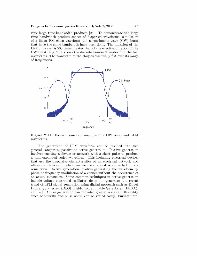
very large time-bandwidth products [25]. To demonstrate the largetime bandwidth product aspect of dispersed waveforms, simulationof a linear FM chirp waveform and a continuous wave (CW) burstthat have the same bandwidth have been done. The duration of theLFM, however is 500 times greater than of the effective duration of theCW burst. Fig. 2.11 shows the discrete Fourier Transform of the twowaveforms. The transform of the chirp is essentially flat over its rangeof frequencies.
b
oτ
π-ω
4ωo b
o τ
π+ω
4 ω
-20
-15
-10
-5
0
d B
Frequency
CW burst
LFM
Figure 2.11. Fourier transform magnitude of CW burst and LFMwaveforms.
The generation of LFM waveform can be divided into twogeneral categories, passive or active generation. Passive generationinvolves exciting a device or network with a short pulse to producea time-expanded coded waveform. This including electrical devicesthat use the dispersive characteristics of an electrical network andultrasonic devices in which an electrical signal is converted into asonic wave. Active generation involves generating the waveform byphase or frequency modulation of a carrier without the occurrence ofan actual expansion. Some common techniques in active generationinclude voltage controlled oscillator, delay line generator and recenttrend of LFM signal generation using digital approach such as DirectDigital Synthesizer (DDS), Field-Programmable Gate Array (FPGA),etc. [26]. Active generation can provided greater waveform flexibilitysince bandwidth and pulse width can be varied easily. Furthermore,
46 Chan and Koo
the waveform is simpler to generate.Processing of LFM waveform can also be divided into two general
classes, namely passive and active processing. Passive processinginvolves the used of a compression network that is conjugate ofexpansion network and is a matched-filtering approach. Activeprocessing involves mixing delayed replicas of the transmitted signalwith the received signal and is a correlation processing approach.The active processing reduces the complexity of system design andhardware implementation.
2.3.4. Matched Filter Response for LFM Waveform
The transmitted signal is given by (2.36)
s(t) = cos[j2π
(fct+ kt2/2
)], −τ/2 ≤ t ≤ τ/2
= 0, elsewhere
The matched filter has an impulse response, h(t), that is time inverseof the signal at receiver input as given below
h(t) = K cos{
2π(fct−
12kt2
)}, −τ/2 ≤ t ≤ τ/2 (2.39)
where K is factor that result in unity gain. Since the echo from thetarget at time to is delayed replica of the transmitted signal, the returnsignal is given as
s(to) = cos{
2π(fc + fdto +
12kt2o
)}(2.40)
where s(to) represent the return echo from target and fd is the shiftedin frequency cause by the Doppler effect.
From above equation, the matched filter characteristics of (2.39),and the convolution integral of (2.33), the general output of matchedfilter can be written as
g(to, ωd) = K
∫ τ/2
−τ/2cos
{(ωc + ωd)t+
12k(2π)t2
}cos {ωc(to − t)
+12k(2π)(to − t)2
}dt (2.41)
where ωc=2πfc and ωd=2πfd.The closed form solution of above equation can be obtained
through a considerable amount of trigonometric and algebraic

Progress In Electromagnetics Research B, Vol. 2, 2008 47
manipulation. The result of this calculation is given as,
g(to, ωd) = G cos{(ωo +
ωd
2
)to
} sin{
ωd+2πkto2 (τ − |to|)
}ωd+2πkto
2
,
−τ/2 ≤ t ≤ τ/2 (2.42)
where |to| is the absolute value of to. Note that the above equation isin the form of sin X
X .
2.3.5. Range Resolution of LFM Waveform
From (2.36), the linear FM transmitted pulse can be written as,
s(t) = Eo cos[j2π
(fct+ kt2
)], −τ/2 ≤ t ≤ τ/2 (2.43)
where Eo is the signal amplitude, fc is the signal carrier frequency andk is the chirp rate. The frequency of the signal sweeps through a band−kτ
2 ≤ (f − fc) ≤ kτ2 so that the bandwidth of the signal, B is equal
to the product of the chirp slope and the pulse duration.The return echo from the target is down converted by shifting
the spectrum of return signal according to the reference signal carrierfrequency and filtering the result to recover only the frequency bandcentred about baseband frequency with bandwidth B. Both in-phaseand quadrature-phase components of the signal can be extracted andthis operation is known as “I, Q detection”. The output of the filteringprocess can be written as,
g(t− to) = E2oBsincπB(t− to) (2.44)
where to is the delay of he return from the point target and time-widthof g(t) is 1/B. Substituting 1/B for τp in Equation (2.3) gives,
ρg =c
2B sin θ(2.45)
The larger bandwidth in linear FM, the better range resolution can beachieved.
2.3.6. Stretch Processor
Active processing can be basically divided into two techniques [24].The first technique is known as “correlation processing” which isnormally used for narrow and medium band radar operation. Thesecond technique is called “stretch processing” or “deramp compression

48 Chan and Koo
processing” and is normally used to process high bandwidth LFMwaveform. The stretch processing technique is employed since it ismuch easier to implement. Others advantages include reduced signalbandwidth, dynamic range increase due to signal compression, andthe baseband frequency offset is directly proportional to the targetrange. Beside that, the correlation processing employed the amplitudemodulating that introduces extra burdens on the transmitter henceincrease the hardware complexity.
The block diagram for a stretch processing receiver is shown inFig. 2.12. The stretch processing consists of the following steps: first ofall the received signals are mixed with a reference signal from the localoscillator (LO). Hence, active-correlation multiplication is conductedat RF followed by lowpass filtering to extract the difference frequencyterms. The signal is split into I and Q components and digitised forfurther processing. The return from each range bin within the selectedrange gate thus corresponding to a pulsed sinusoid at the output of theactive difference mixer. The later the return, the higher the residualfrequency. Pulse compression is completed by performing a spectralanalysis of the difference-frequency output to transform the pulse tonesinto corresponding frequency resolution cells. Spectral analysis isperformed by digitising the difference frequency output and processingit through an FFT.
Low pass filtering
frequency
time
LO
frequency
time
Received Signals
1 2
frequency
time
Correlated Signals
1
2
A/DConversion FFT
Pulsecompressed
output
power
time
Compressed output
Figure 2.12. Stretch pulse compression.
Figure 2.13 shows the frequency against time in derampcompression processing. The TX, REF and RX represent thetransmitted signal, the reference signal, and the received signal froma point targets respectively. The reference signal is generated such

Progress In Electromagnetics Research B, Vol. 2, 2008 49
f
t
τ
τd
fIF
TX
REF
RX
∆t
B
Figure 2.13. Deramp range compression.
that its length ∆t is the timewidth of the slant range swath overwhich returns are expected. The frequency of the reference signalis linearly swept over a RF bandwidth, B. The received signal is areplica of transmitted signal with a time delay τd. From the geometryof Fig. 2.13, the IF frequency, fIF can be written as,
fIF
τd=
B
∆t
or
fIF =B
∆tτd (2.46)
2.4. The SAR Radar Equation
The radar equation for a monostatic radar system can be written as
Pr =PtG
2λ2σ
(4π)3R4(2.47)
wherePr=power received at the antennaPt=power radiated by the antennaG=antenna gainR=distance from radar to the targetλ=operating wavelengthσ=radar target cross sectionSignals received by radar are usually contaminated by noise
due to random modulations of the radar pulse during atmosphericpropagation, or due to fluctuations in the receiving circuits. The signal

50 Chan and Koo
to noise ratio (SNR) is defined as:
SNR =S
No=
PtG2λ2σ
(4π)3R4No(2.48)
The receiver noise can originate within the receiver itself or it mayenter the receiver through the receiving antenna. The thermal noise ofthe receiver can be written as
Thermal noise = kTBn (2.49)
where k is the Boltzmann’s constant and is equal to 1.38×10⁻²³ joulesper degree, T is effective noise temperature, and the equivalent noisebandwidth Bn, in HZ. The total receiver noise is given by
No = FkTBn (2.50)
where F represents the experimentally determine constant called noisefigure. For a target seen against receiver noise, the SNR per pulse isthen:
SNR =PtG
2λ2σ
(4π)3R4kToBnF(2.51)
Hence the SNR after SAR processing, for a point target of crosssection σ at range R is:
SNR =PtG
2λ2σn
(4π)3R4No(2.52)
This improvement in SNR by a factor of n after coherent integration ofsynthetic aperture length. The number of elements, n, which comprisethe synthetic aperture is:
n = Ts.fr (2.53)
where Ts is the time over which the aperture is formed and fr is thepulse repetition frequency. Ts is related to synthetic aperture length,L via:
Ts =L
v=
λR
2vρa sin θo(2.54)
where ρa represent azimuth resolution, fr represent pulse repetitionfrequency, θ is the look angle of the antenna beam and v is the velocity

Progress In Electromagnetics Research B, Vol. 2, 2008 51
of platform. The total number of pulse integrated over coherentintegration time will be
n =frRλ
2ρav sin θo(2.55)
Thus the final form of the SAR radar equation for a point target is:
SNR =PtG
2λ3r
(4π)3R3No2ρav sin θo(2.56)
For a point target in a SAR image, the SNR improves with finerazimuth resolution.
For a distributed target, The radar target cross section can beexpressed in terms of azimuth and range resolution cell, ρa and ρg as,
σ = ρaρgσo (2.57)
where σo is the backscattering coefficient. From (2.56) and (2.57), theSAR radar equation become,
SNR =PtG
2λ3σoρgfr
(4π)3R3No2v sin θo(2.58)
Assuming an initial uncompressed pulse duration of τi and acompressed pulse duration of τc, the pulse compression ratio D canbe written as
D =τiτc
(2.59)
Finally, utilising the relation for the average power P as a function ofpeak power P of (2.52), we obtain
P = Pτifr or P =P
τifi(2.60)
Using relation (2.58) through (2.59) in (2.60), we get
SNR=(P
τifr
)(G2λ2)(ρaρrσo)
(τiτc
)(frRλ
2ρav
)/(4π)3R4(FkTBn) sin θo
(2.61)
where SNR represent the total signal to noise ratio. Simplified the(2.61), we obtain
SNR =PG2λ3ρgσo
(2v)(4π)3kTFR3 sin θo(2.62)

52 Chan and Koo
Rearrange of above equation will result
P =(
(4π)3R3kTF
G2λ2σoρg
) (2vλ
)(SNR) sin θo (2.63)
For strip-mode SAR, the squint angle, θo = 90◦, therefore (2.63) canbe written as
P =(
(4π)3R3kTF
G2λ2σoρg
) (2vλ
)(SNR) (2.64)
Equation (2.64) leads to the conclusion that in SAR systemthe SNR is: 1) inversely proportional to the third power of range;2) independent of azimuth resolution; 3) function of the groundrange resolution; 4) inversely proportional to the velocity; and 5)proportional to the third power of wavelength. From (2.62), increasedresolution in range direction, i.e., smaller ρg, will require increasedtransmitted power. In a number of synthetic array radar this isachieved by pulse compression technique.
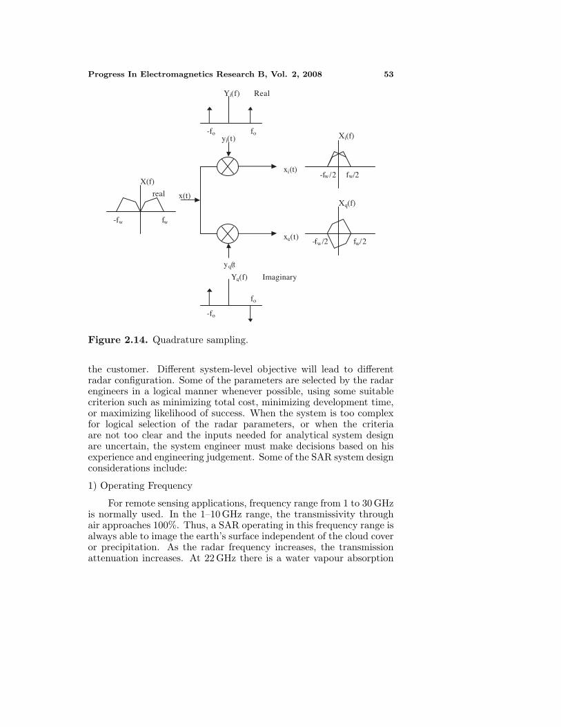
2.5. In Phase and Quadrature (IQ) Sampling
The sampling rate of the analogue signal can be reduced by separatingthe signal into two waveforms, and sampling each channel at itsNyquist rate. This is based on the principle that a signal can beexpressed in terms of two waveforms called quadrature functions [22].The concept of IQ sampling is illustrated in Fig. 2.14.
An input waveform x(t) with a bandwidth fw is multiple by acosine in one channel and a phase shifted cosine in the other channel.The second cosine is phased shifted by 90◦ (or one quadrant). Thecosine term is assigned to the real axis and is known as in-phase term.The second channel is shifted by one quadrant and is commonly calledthe quadrature term. X(f), Yi(f) and Yq(f) are the Fourier transformof x(t), yi(t) and yq(t) respectively.
The multiplication in the time domain is equivalent to theconvolution in the frequency domain. This results each of twoquadrature functions occupies only one half the bandwidth of originalsignal. Therefore it is possible to sample each quadrature signal at onehalf sampling rate required to sampled the original signal.
3. SAR SYSTEM DESIGN CONSIDERATION
The parameters of a SAR system depend on the primary goal of theproject and are determined cooperatively by the system engineer and
Progress In Electromagnetics Research B, Vol. 2, 2008 53
Yi(f) Real
fo-fo
Yq(f) Imaginary
-fo
fo
yi(t)
yq(t
x(t)
X(f)
fw-fw
xi(t)
xq(t)
Xi(f)
fw/2-fw/2
Xq(f)
fw/2-fw/2
real
Figure 2.14. Quadrature sampling.
the customer. Different system-level objective will lead to differentradar configuration. Some of the parameters are selected by the radarengineers in a logical manner whenever possible, using some suitablecriterion such as minimizing total cost, minimizing development time,or maximizing likelihood of success. When the system is too complexfor logical selection of the radar parameters, or when the criteriaare not too clear and the inputs needed for analytical system designare uncertain, the system engineer must make decisions based on hisexperience and engineering judgement. Some of the SAR system designconsiderations include:
1) Operating Frequency
For remote sensing applications, frequency range from 1 to 30 GHzis normally used. In the 1–10 GHz range, the transmissivity throughair approaches 100%. Thus, a SAR operating in this frequency range isalways able to image the earth’s surface independent of the cloud coveror precipitation. As the radar frequency increases, the transmissionattenuation increases. At 22 GHz there is a water vapour absorption
54 Chan and Koo
band that reduces transmission to about 85%.
2) Modulations
In SAR system, there are basically three types of widely usedmodulation schemes: pulse, LFM or chirp and phase coded. Pulsesystem is used in older generation radar. Modern radar usesLFM waveform to increase range resolution when long pulses arerequired to get reasonable signal to noise ratio. The same averagetransmitting power as in a pulse system can be achieved with lowerpeak amplitude. The LFM configuration is employed in this projectsince it gives better sensitivity without sacrificing range resolution andease of implementation. The lower peak power allows for the useof commercially available microwave components that have moderatepeak power handling capability. Phase coded modulation is notprefer due to it’s difficulty to generate. Phase coded modulationnormally used for long duration waveforms and when jamming maybe a problem.
3) Mode of Operation
Available data acquisition mode includes strip-mapping, squintmode, spotlight mode, ScanSAR, interferometry and polarimetricSAR. Spotlight mode SAR provides high-resolution image but involvescomplex hardware and processing algorithm. Squint mode SAR is usedto image while maneuvering. It usually employed in military aircraft.ScanSAR is normally used in spaceborne SAR in order to increase theswath width. It requires powerful computation hardware. Polarimetricsystem capable of measuring scattering matrix S of target whereasinterferometry SAR is the latest technology developed with capabilityof measuring terrain high and constructing three dimensional image.Hardware design of interferometry and polarimetric SAR is morecomplicated.
4) Polarisation
Conventional SAR system employed single polarisation such as VVor HH to acquire information from earth. For remote sensing of earthterrain such as oil palm plantation or tropical forest, single polarisationis sufficient. A device which measures the full polarisation responseof the scattered wave is called a polarimeter. Polarimetric systemsdiffer from conventional system in that they are capable of measuringthe complete scattering matrix of the remotely sensed media. Byhaving the knowledge of the complete scattering matrix, it is possibleto calculate the backscattered signal for any given combination ofthe transmitting and receiving antennas. This process is called the

Progress In Electromagnetics Research B, Vol. 2, 2008 55
polarisation synthesis, which is an important technique used in terrainclassification [27–29].
5) Dynamic Range of Backscattering Coefficient σ◦
The required system sensitivity is determined based on the variouscategories of earth terrain to be mapped such as man made target,ocean, sea-ice, forest, natural vegetation and agriculture, geologicaltargets, mountain, land and sea boundary. From the open literatures,the typical value of σ◦ falls in the range of +20 dB to −40 dB [30, 31].For vegetation the typical value of σ◦ vary from +0 dB to −20 dB.
6) Operating Platform
Basically SAR systems can be separated into two groups: airbornesystem operating on variety of aircraft and spaceborne systemoperating on satellite or space shuttle platforms. Spaceborne SARshave smaller range of incidence angle and larger swath width, but highdata rate is a problem. Whereas airborne SARs illuminated smallerfootprint on the earth and the data rate is much lower.
7) Spatial Resolution
Typical resolution of airborne SAR range from 1 m to 20 m [15].It depends mostly on the application requirements. Table below showssome science applications vs. resolutions of airborne SAR.
Table 3.1. Science applications vs. resolution requirement.
Discipline ResolutionVegetation classification 5–20 m
Soil Moisture and Salinity 5–50 mHydrology 5–20 m
Oceanography 50–200 mArchaeology 2–20 m
8) Swath Width and Range of Incident Angle to be covered
From the open literature, the swath width for airborne SAR rangefrom 5 km to 60 km depends on altitude of operating platform andincidence angle. From the open literatures, the incident angle from 0◦–80◦ is utilised by present airborne SARs. The backscattering coefficientof nature targets such as soil, grass and vegetable are maintainedalmost constant over the incident angle of 40◦ to 60◦ [1, 32].

56 Chan and Koo
9) Pulse Repetition Frequency (PRF)
The upper limit of PRF is attained from a consideration of themaximum mapping range and the fact that the return pulse fromthis range should come within the interpulse period [21]. In orderto adequately sample the Doppler bandwidth, the radar must be pulsewith a PRF greater or equal to this bandwidth. Combination of lowerand upper limit, we obtained
2v�
≤ PRF ≤ c
2Rfar
where Rfar is the far range from the airborne platform.
10) Antenna
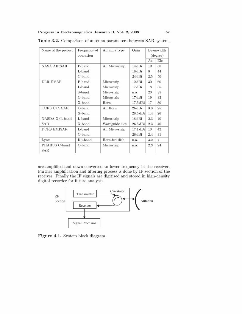
Yagi, slotted-waveguide, horn, dish, and microstrip antennas havefound some applications in SAR one time or another. Table 3.2 showsa summary of some selected SAR systems. Yagi is suited for lowerfrequency applications, while dish is suited for very high frequencyapplication. Modern civilian SAR system generally operate in L- C-and X-band, where slotted-waveguide and microstrip antennas providethe best performance.
4. DESIGN PARAMETERS
The design consideration in Section 3 can be used as the basic guidelineto select the suitable microwave system parameters. Basically, thesystem hardware consists of (i) the microwave components such asantenna, oscillator, mixer, power amplifier and circulator, and (ii)the low frequency electronics components such as integrated circuits,resistors and capacitors. The design of the microwave subsystem isgenerally more difficult to handle. Therefore, the microwave subsystemwas given more attention in the initial stage of the design. The lowfrequency sections were carefully designed to match the microwave’sspecifications.
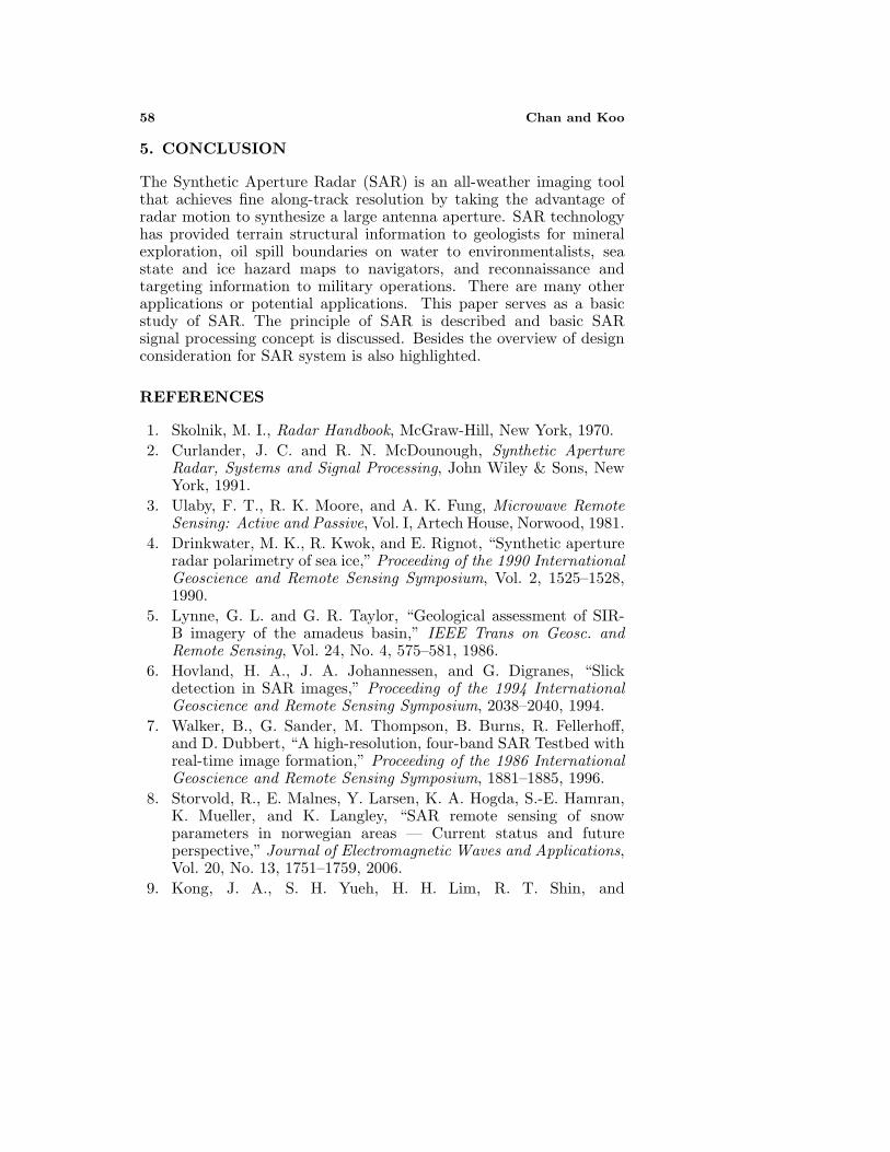
Subsystem level design determines the requirements of SARsubsystem. The requirements will be based on the design parametersdecided in Section 3. The radar subsystem can be functionally dividedinto three assemblies: (i) Transmitter; (ii) Receiver; and (iii) antenna.Each of these assemblies can be further divided into subassembliesand components. Fig. 4.1 shows the block diagram of the SARsystem. The transmitter generated the required signal and transmittedvia an antenna. Part of the energy is intercepted by the targetand reflected back to the receiving antenna. The received echoes
Progress In Electromagnetics Research B, Vol. 2, 2008 57
Table 3.2. Comparison of antenna parameters between SAR system.
Name of the project Frequency of Antenna type Gain Beamwidth
operation (degree)
Az Ele
NASA AIRSAR P-band All Microstrip 14 dBi 19 38
L-band 18 dBi 8 44
C-band 24 dBi 2.5 50
DLR E-SAR P-band Microstrip 12 dBi 30 60
L-band Microstrip 17 dBi 18 35
S-band Microstrip n.a. 20 35
C-band Microstrip 17 dBi 19 33
X-band Horn 17.5 dBi 17 30
CCRS C/X SAR C-band All Horn 26 dBi 3.3 25
X-band 28.5 dBi 1.4 26
NASDA X/L-band L-band Microstrip 18 dBi 2.3 40
SAR X-band Waveguide-slot 26.5 dBi 2.3 40
DCRS EMISAR L-band All Microstrip 17.1 dBi 10 42
C-band 26 dBi 2.4 31
Lynx Ku-band Horn-fed dish n.a. 3.2 7
PHARUS C-band C-band Microstrip n.a. 2.3 24
SAR
are amplified and down-converted to lower frequency in the receiver.Further amplification and filtering process is done by IF section of thereceiver. Finally the IF signals are digitised and stored in high-densitydigital recorder for future analysis.
Transmitter
Receiver
Signal Processor
RFSection Antenna
Circulator
Figure 4.1. System block diagram.
58 Chan and Koo
5. CONCLUSION
The Synthetic Aperture Radar (SAR) is an all-weather imaging toolthat achieves fine along-track resolution by taking the advantage ofradar motion to synthesize a large antenna aperture. SAR technologyhas provided terrain structural information to geologists for mineralexploration, oil spill boundaries on water to environmentalists, seastate and ice hazard maps to navigators, and reconnaissance andtargeting information to military operations. There are many otherapplications or potential applications. This paper serves as a basicstudy of SAR. The principle of SAR is described and basic SARsignal processing concept is discussed. Besides the overview of designconsideration for SAR system is also highlighted.
REFERENCES
1. Skolnik, M. I., Radar Handbook, McGraw-Hill, New York, 1970.2. Curlander, J. C. and R. N. McDounough, Synthetic Aperture
Radar, Systems and Signal Processing, John Wiley & Sons, NewYork, 1991.
3. Ulaby, F. T., R. K. Moore, and A. K. Fung, Microwave RemoteSensing: Active and Passive, Vol. I, Artech House, Norwood, 1981.
4. Drinkwater, M. K., R. Kwok, and E. Rignot, “Synthetic apertureradar polarimetry of sea ice,” Proceeding of the 1990 InternationalGeoscience and Remote Sensing Symposium, Vol. 2, 1525–1528,1990.
5. Lynne, G. L. and G. R. Taylor, “Geological assessment of SIR-B imagery of the amadeus basin,” IEEE Trans on Geosc. andRemote Sensing, Vol. 24, No. 4, 575–581, 1986.
6. Hovland, H. A., J. A. Johannessen, and G. Digranes, “Slickdetection in SAR images,” Proceeding of the 1994 InternationalGeoscience and Remote Sensing Symposium, 2038–2040, 1994.
7. Walker, B., G. Sander, M. Thompson, B. Burns, R. Fellerhoff,and D. Dubbert, “A high-resolution, four-band SAR Testbed withreal-time image formation,” Proceeding of the 1986 InternationalGeoscience and Remote Sensing Symposium, 1881–1885, 1996.
8. Storvold, R., E. Malnes, Y. Larsen, K. A. Hogda, S.-E. Hamran,K. Mueller, and K. Langley, “SAR remote sensing of snowparameters in norwegian areas — Current status and futureperspective,” Journal of Electromagnetic Waves and Applications,Vol. 20, No. 13, 1751–1759, 2006.
9. Kong, J. A., S. H. Yueh, H. H. Lim, R. T. Shin, and

Progress In Electromagnetics Research B, Vol. 2, 2008 59
J. J. van Zyl, “Classification of earth terrain using polarimetricsynthetic aperture radar images,” Progress In ElectromagneticsResearch, PIER 03, 327–370, 1990.
10. Thompson, T. W., A User’s Guide for the NASA/JPLSynthetic Aperture Radar and the NASA/JPL L- and C-bandScatterometers, 83–38, JPL Publication, 1986.
11. Held, D. N., W. E. Brown, A. Freeman, J. D. Klein,H. Zebker, T. Sato, T. Miller, Q. Nguyen, and Y. L. Lou,“The NASA/JPL multifrequency, multipolarisation airborne SARsystem,” Proceeding of the 1988 International Geoscience andRemote Sensing Symposium, 345–349, 1988.
12. Thompson, D. G., D. V. Arnold, and D. G. Long, “YSAR: Acompact, low-cost synthetic aperture radar,” Proceeding of the1996 International Geoscience and Remote Sensing Symposium,1892–1894, 1996.
13. Livingstone, C. E., A. L. Gray, R. K. Hawkins, and R. B. Olsen,“CCRS C/X-airborne synthetic aperture radar: An R&D tool forthe ERS-1 time frame,” IEEE Aerospace and Electronic SystemsMagazine, Vol. 3, No. 10, 11–20, 1988.
14. Walker, B., G. Sander, M. Thompson, B. Burns, R. Fellerhoff,and D. Dubbert, “A high-resolution, four-band SAR Testbed withreal-time image formation,” Proceeding of the 1986 InternationalGeoscience and Remote Sensing Symposium, 1881–1885, 1996.
15. Birk, R., W. Camus, E. Valenti, and W. J. McCandles, “Syntheticaperture radar imaging systems,” IEEE Aerospace and ElectronicSystems Magazine, Vol. 10, No. 11, 15–23, 1995.
16. Madsen, S. N., E. L. Christensen, N. Skou, and J. Dall, “TheDanish SAR system: Design and initial tests,” IEEE Trans. onGeosc. and Remote Sensing, Vol. 29, No. 3, 417–426, 1991.
17. Thompson, D. G., D. V. Arnold, D. G. Long, G. F. Miner,M. A. Jensen, “YINSAR: A compact, low-cost interferometricsynthetic aperture radar,” Proceeding of the 1998 InternationalGeoscience and Remote Sensing Symposium, 1920–1922, 1998.
18. Way, J. and E. A. Smith, “The evolution of synthetic apertureradar systems and their progression to the EOS SAR,” IEEETransactions on Geoscience and Remote Sensing, Vol. 29, Issue 6,962–985, 1991.
19. Nemoto, Y., H. Nishino, M. Ono, H. Mizutamari, andK. Nishikawa, K. Tanaka, “Japanese Earth Resources Satellite-1 synthetic aperture radar,” Proceedings of the IEEE, Vol. 79,Issue 6, 800–809, 1991.

60 Chan and Koo
20. Jordan, R. L., B. L. Huneycutt, and M. Werner, “The SIR-C/X-SAR synthetic aperture radar system,” IEEE Transactions onGeoscience and Remote Sensing, Vol. 33, Issue 4, 829–839, 1995.
21. Hovanessian, S. A., Introduction to Synthetic Array and ImagingRadars, Artech House, Dedham, 1980.
22. Kamath, J., “Real time imaging systems for synthetic apertureradar using coarse quantized correlators with VLSI realisation,”Doctoral dissertation, University of Idaho, Idaho, USA, 1995.
23. Di Cenzo, A., “A new look at nonseparable synthetic apertureradar processing,” IEEE Trans. on Aerospace and ElectronicSystems, Vol. 24, No. 3, 218–223, 1988.
24. Mahafza, B. F., Introduction to Radar Analysis, CRC Press, NewYork, 1998.
25. Jakowatz, C. V., D. E. Wahl, P. H. Eichel, D. C. Ghiglia, andP. A. Thompson, Spotlight-mode Synthetic Aperture Radar: ASignal Processing Approach, Kluwer Academic Publishers, Boston,1996.
26. Chan, Y., K. and S., Y. Lim, “Synthetic aperture radar (SAR)signal generation,” Progress In Electromagnetics Research B,accepted for publication.
27. Zebker, H. A., J. J. van Zyl, and D. Held, “Imagingradar polarimetry from wave synthesis,” Journal of GeophysicalResearch, Vol. 92, No. B1, 683–701, 1987.
28. Van Zyl, J. J. and H. A. Zebker, “Imaging radar polarimetry,”Progress In Electromagnetics Research, PIER 03, 277–326, 1990.
29. Evans, D. L. and J. J. van Zyl, “Polarimetric imaging radar:Analysis tools and applications,” Progress In ElectromagneticsResearch, PIER 03, 371–389, 1990.
30. Hyyppa, J., J. Pulliainen, K. Heiska, and M. Hallikainen,“Statistics of backscattering source distribution of borealconiferous forests at C- and X-band,” Proceeding of the 1986International Geoscience and Remote Sensing Symposium, Vol. 1,241–242, 1994.
31. Pulliainen, J. T., K. Heiska, J. Hyyppa, and M. T. Hallikainen,“Backscattering Properties of boreal forests at the C- and X-bands,” IEEE Trans on Geosc. and Remote Sensing, Vol. 32,No. 5, 1041–1050, 1994.
32. Ulaby, F. T. and T. F. Bush, “Cropland inventories using anorbital imaging radar,” Remote Sensing Laboratory, 1977.