Animation of Humanlike Characters: Dynamic Motion Filtering with aPhysically Plausible Contact Model

Nancy S. Pollard and Paul S. A. Reitsma

Brown University∗

Abstract

Data-driven techniques for animation, where motion captured froma human performer is “played back” through an animated humancharacter, are becoming increasingly popular in computer graphics.These techniques are appealing because the resulting motion of-ten retains the natural feel of the original performance. Data-driventechniques have the disadvantage, however, that it is difficult to pre-serve this natural feel when the motion is edited, especially when itis edited by a software program adapting the motion for new uses(e.g. to animate a character traveling over uneven terrain). In fact,many current techniques for motion editing do not preserve basiclaws of physics. We present a dynamic filtering technique for im-proving the physical realism of motion for animation. As a specificexample, we show that this filter can improve the physical realismof automatically generated motion transitions. Our test case is thephysically challenging transition contained in a double kick con-structed by merging two single kicks.

1 Introduction

Motion editing is a “hot topic” in computer animation, es-pecially animation of human characters. We have access toa growing base of realistic captured human motion data, andmany researchers believe that this data will allow us to finallycreate believable digital humans. In a data-driven approachto animation, a continuous stream of motion is created byclipping, splicing, blending, and scaling existing motion se-quences to allow the character to accomplish a specific set ofgoals. For example, a character’s motion through an obstaclecourse may be created by assembling jumping, running, andclimbing segments taken from a motion capture database.

Motion captured from human actors is physically realis-tic, at least within the accuracy of the measurements, but theprocess of blending, patching, and adjusting this motion in-troduces artifacts. Motion that has been edited is typicallyprocessed to reduce these artifacts. The tools that producethe best results are iterative: an artist will make repeatedmanual adjustments to achieve a desired effect, or an offlineprocess will optimize the motion based on an objective suchas minimal energy.

In certain domains, such as automatic animation of char-acters in virtual environments, an iterative approach is notappropriate. In a virtual environment, processing time is lim-ited, and the character’s motion may change at any time, dueto user actions or events in the environment. The best we canhope for is to put the motion through one or more filters.

1email: [nsp|psar]@cs.brown.edu

The most common motion filters are kinematic. Kine-matic filters adjust the pose of a character on a frame byframe basis to maintain constraints such as keeping thestance foot planted firmly on the ground or ensuring thatthe character’s center of mass projects to a point within itsbase of support. More recently, dynamic filters and track-ing controllers have begun to appear in the animation lit-erature [14] [15]. Dynamic filters and tracking controllerscan be used to maintain physical constraints, such as keep-ing torques within their limits and keeping required contactforces within a reasonable friction cone.

This paper describes a dynamic filter for processing mo-tion for improved physical realism. Our contribution overexisting techniques is to combine feed-forward tracking witha friction-based model of contact between the character andthe environment. Such a model allows sliding when appro-priate and rejects motions that would not be plausible for aphysical system such as a robot to carry out. We show ex-amples of success and failure of our filter with a physicallychallenging motion where a single kick has been altered tocreate a double kick (Figure 3).

2 Background

Iterative kinematic techniques for motion editing allow theuser to adjust parameters of the motion, such as the pose ata specific frame, and propagate the effects of the adjustmentthrough the entire motion. Gleicher [6] solves for the motiondisplacement that minimizes the difference from the sourcemotion. Lee and Shin [8] use a hierarchical B-spline rep-resentation of motion to limit changes to user-specified fre-quency bands. Ko and Badler [7] use inverse kinematics tomodify motion while considering balance. van de Panne [12]and the Character Studio software product [4] allow a user tocontrol footprint locations. Others [11], [1], [10] have devel-oped signal processing techniques for blending and alteringexample motion. These techniques largely rely on the artist’seye to ensure that the results appear physically plausible.

Constrained optimization of dynamic simulations wasintroduced to the graphics community by Witkin andKass [13], who optimized motion for a jumping lamp. In thebiomechanics community, Pandy has optimized lower bodymotion for maximal height jumping and for minimal energywalking. His models involved 54 muscles, 864 degrees offreedom, and use of parallel computers to keep computation

time to manageable levels. Popovi´c and Witkin [9] show thatoptimization times on the order of minutes can be obtainedfor human motion when the optimization is performed on asimplified version of the character. These techniques resultin motion that obeys physical laws (as well as possible), butthey require search through a high dimensional space and arenot suited for use in a virtual environment where a charac-ter’s motion and goals may be changing.

A tracking controller is used by Zordan [15], who en-hances simple PD tracking with a balance controller and col-lision simulations for convincing behavior in actions suchas drumming and punching. Dynamic tracking was usedby Yamane and Nakamura [14], who place virtual links atlocations of ground contact, and find a least squares solu-tion for acceleration of the constrained system to best matchthe motion they are tracking. The contribution of our workover theirs is to present an alternative approach that modelscharacter-environment contact as contact with friction andallows complex interactions such as shifting the weight andpivoting to be easily handled.

3 Problem Setup

The examples in this paper draw on a motion editing sys-tem we have developed. This section describes how motionwas captured, edited, and fit to a physical model. It also de-scribes our model of contact between the character and theenvironment.

3.1 Motion Capture Data

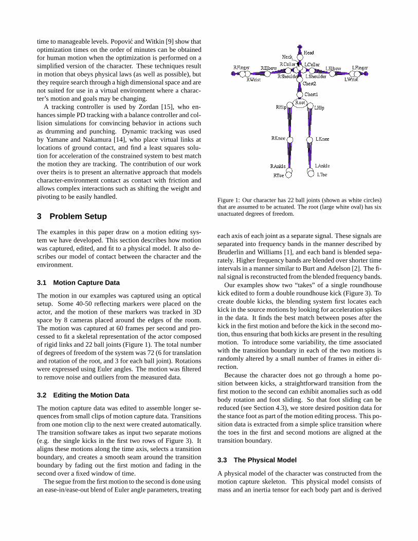
The motion in our examples was captured using an opticalsetup. Some 40-50 reflecting markers were placed on theactor, and the motion of these markers was tracked in 3Dspace by 8 cameras placed around the edges of the room.The motion was captured at 60 frames per second and pro-cessed to fit a skeletal representation of the actor composedof rigid links and 22 ball joints (Figure 1). The total numberof degrees of freedom of the system was 72 (6 for translationand rotation of the root, and 3 for each ball joint). Rotationswere expressed using Euler angles. The motion was filteredto remove noise and outliers from the measured data.

3.2 Editing the Motion Data

The motion capture data was edited to assemble longer se-quences from small clips of motion capture data. Transitionsfrom one motion clip to the next were created automatically.The transition software takes as input two separate motions(e.g. the single kicks in the first two rows of Figure 3). Italigns these motions along the time axis, selects a transitionboundary, and creates a smooth seam around the transitionboundary by fading out the first motion and fading in thesecond over a fixed window of time.

The segue from the first motion to the second is done usingan ease-in/ease-out blend of Euler angle parameters, treating

Figure 1: Our character has 22 ball joints (shown as white circles)that are assumed to be actuated. The root (large white oval) has sixunactuated degrees of freedom.

each axis of each joint as a separate signal. These signals areseparated into frequency bands in the manner described byBruderlin and Williams [1], and each band is blended sepa-rately. Higher frequency bands are blended over shorter timeintervals in a manner similar to Burt and Adelson [2]. The fi-nal signal is reconstructed from the blended frequency bands.

Our examples show two “takes” of a single roundhousekick edited to form a double roundhouse kick (Figure 3). Tocreate double kicks, the blending system first locates eachkick in the source motions by looking for acceleration spikesin the data. It finds the best match between poses after thekick in the first motion and before the kick in the second mo-tion, thus ensuring that both kicks are present in the resultingmotion. To introduce some variability, the time associatedwith the transition boundary in each of the two motions israndomly altered by a small number of frames in either di-rection.

Because the character does not go through a home po-sition between kicks, a straightforward transition from thefirst motion to the second can exhibit anomalies such as oddbody rotation and foot sliding. So that foot sliding can bereduced (see Section 4.3), we store desired position data forthe stance foot as part of the motion editing process. This po-sition data is extracted from a simple splice transition wherethe toes in the first and second motions are aligned at thetransition boundary.

3.3 The Physical Model

A physical model of the character was constructed from themotion capture skeleton. This physical model consists ofmass and an inertia tensor for each body part and is derived

Figure 2: Example of contact force basis vectors. (Left) Assumethe entire toe is in contact with the ground. The contact area is sam-pled with points on the boundary of the toe geometry, and (Right)force basis vectors are generated to span the friction pyramid ateach contact point. This example has sixteen force basis vectors,four for each of the four sample contact points. If coefficients forall sixteen basis vectors are positive, the force applied by the footwill fall within given friction limits.

from the total mass of the actor, a fit of a geometric modelto the skeleton, and body part density information measuredfrom cadavers[3].

3.4 Contact Forces

A Coulomb model of friction is assumed for contact betweenthe character and its environment. At each frame of the mo-tion, the system checks for collisions between the charac-ter and its environment and selects a discrete set of contactpoints to represent each contact region. A set of basis forcesis constructed at each contact point to approximate the fric-tion cone at that point with a friction pyramid (Figure 2).External forces are assumed to only be applied along thesebasis directions.

4 Filtering the Motion

Given motion data that has been captured and edited as de-scribed above, the job of the dynamic filter is to keep the feetplanted on the ground and filter out impossible forces andtorques. If the foot should pivot or slide, we allow it to doso. If the motion cannot be achieved using legal forces andfeedforward control, the filter fails to correct the motion (i.e.the character falls).

To filter the motion, we start out in an initial state extractedfrom the data and simulate forward in time. At each step,our goal is to find accelerations and applied forces that (1)move the character toward its state in the next frame of themeasured motion, (2) require zero root force and torque, asthese joints are not actuated, and (3) use forces only withinthe friction cones, if desired.

Section 4.1 outlines the dynamics equations we use. Sec-tion 4.2 describes a filter that tracks joint angles as wellas possible, computing contact forces along the way. Sec-tion 4.3 describes how position tracking is added, to keepthe character’s stance foot fixed to the ground, for example.

4.1 Dynamics Equations

The equations of motion with no external forces except grav-ity are

Q = Hq + C (1)

whereH is the mass matrix,C includes velocity effects andgravity terms,q are accelerations of system state parameters,andQ are generalized forces.

We add the effect of contact forces as follows:

Q = Hq + C + Mf (2)

wheref is a vector of force coefficients andM maps forcecoefficients to generalized forces based on the current con-tact geometry. The size off and the interpretation of eachof the coefficients vary depending on how the character con-tacts the environment. Figure 2 shows how basis forces werecomputed for the examples in this paper.

VectorC and matricesH andM are computed by adapt-ing the technique described in [5]: given the character’s cur-rent state (q, q), C is set to the value ofQ computed whenfandq are zero; each columni of H is set to the value(Q−C)whenf is zero andq is δi (value 1 for elementi and 0 forall other elements); each columni of M is set to the value(Q − C) whenq is zero andf is δi.

4.2 Pose Tracking

Motion is tracked by numerically integrating generalized ac-celerations over time. Generalized accelerations are com-puted with two goals in mind: closely match the original mo-tion and eliminate undesirable (physically impossible) rootforces and torques.

The tracking process has four steps. The first step is to cal-culate desired accelerationsqDES(t) that will result in closetracking of the given motion and recovery from tracking er-rors. ThisqDES(t) will be unrealistic if it requires forcesand torques to be applied at the root, which is unactuated.Root generalized forcesQroot are computed fromqDES(t).Forces at the contact points are then computed to reduce oreliminateQroot. AccelerationsqDES(t) are then adjusted toeliminate any root forces and torques that remain. These fourtasks are described below.

4.2.1 Computing Desired Accelerations

Desired accelerationqDES(t) includes root translational ac-celeration, root rotational acceleration, and joint rotationalaccelerations:

qDES(t) =

xroot,DES(t)ωroot,DES(t)ω0,DES(t)

...ωn,DES(t)

(3)

wheren is the number of actuated joints of the character.Desired acceleration is computed from the data and position

and velocity errors. For root translational accelerationxroot:

xroot,DES(t) = xroot,DATA(t) +kx(xroot,DATA(t) − xroot(t)) +bx(xroot,DATA(t) − xroot(t)) (4)

wherekx andbx are stiffness and damping coefficients andxroot,DATA, xroot,DATA, and xroot,DATA are the transla-tional position, velocity, and acceleration of the root in thedata we are tracking.

For root and joint angular accelerationω:

ωi,DES(t) = ωi,DATA(t) +kω(v∆θ)i,CORR +bω(ωi,DATA(t) − ωi(t)) (5)

wherekω andbω are stiffness and damping coefficients andωi,DATA(t) and ωi,DATA(t) are the angular velocity andacceleration for the root or jointi found in the data weare tracking. Parameter(v∆θ)i,CORR is the rotation re-quired to correct error at the root or at jointi, equivalent toqi,DATA(t)q−1

i (t) in angle-weighted axis format.The data we are tracking contains only position informa-

tion. Velocities and accelerations are obtained using simplefinite differences so that Euler integration with no constraintson accelerations would result in the original dataset.

4.2.2 Computing Generalized Forces

Given qDES(t), root generalized forces are computed whenf = 0:

Qroot =[

froot(t)τroot(t)

]= HrootqDES(t) + Croot (6)

whereQroot, Hroot, andCroot are the first six rows ofQ,H , andC, andfroot(t) andτroot(t) are the required forceand torque at the root of the character.

4.2.3 Computing Contact Forces to Support the Root

Qroot in equation 6 represents undesirable forces andtorques, because the root joint is not actuated. To track thedata in a physically plausible way requires finding contactforces to eliminateQroot if possible. In other words, we seekcontact forces to support the desired motion of the character.The following equation is solved forf :

Mrootf = −Qroot (7)

whereMroot is the first six rows of M.If friction cone constraints are not important, equation 7

can be solved using least squares. If contact forces must fallwithin friction cones at the contacts, least squares cannot beused, because it may result in negative coefficients, whichwould violate friction cone constraints.

We have had good success with a simple, greedy iterativetechnique for computingf . At each step of the iteration,

the single force coefficient that moves most directly towarda solution is modified. Coefficients can be either increasedor decreased in an iteration step, but they are constrainedto remain greater than or equal to zero. Iteration continuesto within some small distanceε of the solution or until aniteration step increases the distance to the goal.

4.2.4 Adjusting Acceleration to Eliminate Root Forces

Once f has been computed,qDES(t) is altered to eliminateany root forces and torques that remain. The following equa-tion is solved for∆q using least squares:

Hroot∆q = −Qroot − Mrootf (8)

The new acceleration is:

q′DES(t) = qDES(t) + ∆q (9)

Value q′DES(t) is used to integrate forward one frame of the

animation.

4.3 Reference Point Tracking

Unconstrained tracking results in motion that is close to thereference motion and maintains physical plausibility as de-fined here. Frequently some aspects of the motion are moreimportant than others, however, such as having the stancefoot behave as though it is firmly connected to the ground.We track one or more points attached to the character with astiffer system than that used to track joint angles.

Assumec reference point position signals, extracted fromthe motion data or some other source and collected into asingle vectorrDATA(t):

rDATA(t) =

r0(t)r1(t)

...rc(t)

(10)

DerivativesrDATA(t) andrDATA(t) are computed using fi-nite differences.

The desired acceleration of the reference pointsrDES(t)is

rDES(t) = rDATA(t) +kr(rDATA(t) − r(t)) +br(rDATA(t) − r(t)) (11)

wherekr andbr are stiffness and damping used for referencepoint tracking.

The expected acceleration of the reference pointsrEXP (t)is defined based on the JacobianJ(q) relating state velocitiesto reference point velocities:

r(t) = J(q)q(t) (12)

rEXP (t) = J(q)q(t) + Jq′DES(t) (13)

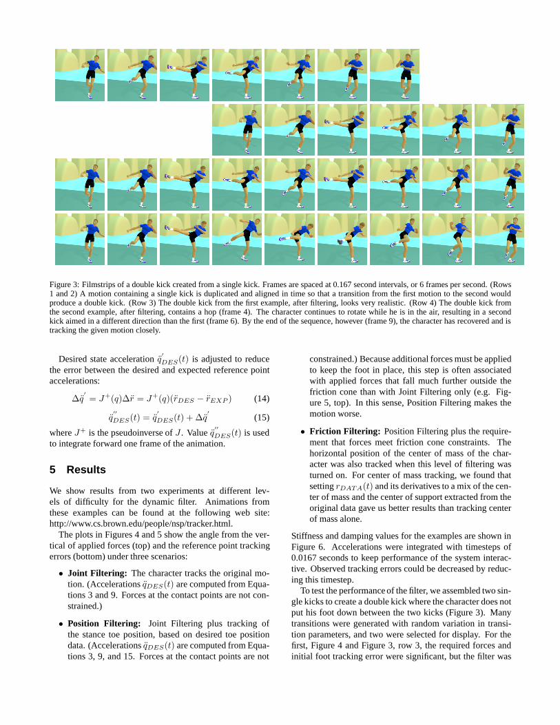
Figure 3: Filmstrips of a double kick created from a single kick. Frames are spaced at 0.167 second intervals, or 6 frames per second. (Rows1 and 2) A motion containing a single kick is duplicated and aligned in time so that a transition from the first motion to the second wouldproduce a double kick. (Row 3) The double kick from the first example, after filtering, looks very realistic. (Row 4) The double kick fromthe second example, after filtering, contains a hop (frame 4). The character continues to rotate while he is in the air, resulting in a secondkick aimed in a different direction than the first (frame 6). By the end of the sequence, however (frame 9), the character has recovered and istracking the given motion closely.

Desired state accelerationq′DES(t) is adjusted to reduce

the error between the desired and expected reference pointaccelerations:

∆q′= J+(q)∆r = J+(q)(rDES − rEXP ) (14)

q′′DES(t) = q

′DES(t) + ∆q

′(15)

whereJ+ is the pseudoinverse ofJ . Valueq′′DES(t) is used

to integrate forward one frame of the animation.

5 Results

We show results from two experiments at different lev-els of difficulty for the dynamic filter. Animations fromthese examples can be found at the following web site:http://www.cs.brown.edu/people/nsp/tracker.html.

The plots in Figures 4 and 5 show the angle from the ver-tical of applied forces (top) and the reference point trackingerrors (bottom) under three scenarios:

• Joint Filtering: The character tracks the original mo-tion. (AccelerationsqDES(t) are computed from Equa-tions 3 and 9. Forces at the contact points are not con-strained.)

• Position Filtering: Joint Filtering plus tracking ofthe stance toe position, based on desired toe positiondata. (AccelerationsqDES(t) are computed from Equa-tions 3, 9, and 15. Forces at the contact points are not

constrained.) Because additional forces must be appliedto keep the foot in place, this step is often associatedwith applied forces that fall much further outside thefriction cone than with Joint Filtering only (e.g. Fig-ure 5, top). In this sense, Position Filtering makes themotion worse.

• Friction Filtering: Position Filtering plus the require-ment that forces meet friction cone constraints. Thehorizontal position of the center of mass of the char-acter was also tracked when this level of filtering wasturned on. For center of mass tracking, we found thatsettingrDATA(t) and its derivatives to a mix of the cen-ter of mass and the center of support extracted from theoriginal data gave us better results than tracking centerof mass alone.

Stiffness and damping values for the examples are shown inFigure 6. Accelerations were integrated with timesteps of0.0167 seconds to keep performance of the system interac-tive. Observed tracking errors could be decreased by reduc-ing this timestep.

To test the performance of the filter, we assembled two sin-gle kicks to create a double kick where the character does notput his foot down between the two kicks (Figure 3). Manytransitions were generated with random variation in transi-tion parameters, and two were selected for display. For thefirst, Figure 4 and Figure 3, row 3, the required forces andinitial foot tracking error were significant, but the filter was

able to fix these errors to create visually plausible motion.

-1000

-500

0

500

1000

1500

2000

2500

3000

3500

0 500 1000 1500 2000 2500 3000 3500 4000 4500

Ver

tical

For

ce

Horizontal Force

Ground Forces, Example 1

Joint FilteringPositon FilteringFriction Filtering

Friction Boundary

0

0.05

0.1

0.15

0.2

0.25

0.3

0 40 80 120 160 200

Tra

ckin

g E

rror

(cm

)

Frame

Toe Position Tracking Error, Example 1

Joint FilteringPosition FilteringFriction Filtering

Figure 4: Modified data, double kick formed from two single kicks.(Top) Effects of filtering on applied forces. Horizontal force mag-nitude is plotted vs. vertical force for each frame of the motion.Forces below and to the right of the solid line require an unrealis-tic friction coefficient (greater than 1.0). Forces with Joint Filtering(filled circles) and Position Filtering (boxes) fall outside the frictioncone boundary. When Friction Filtering is turned on (stars), the dy-namic filter keeps ground contact forces within the friction cone atthe contacts. (Bottom) Tracking errors for this motion are small forboth Position and Friction Filtering.

The second example, Figure 5 and Figure 3, row 4, is moreaggressive because the amount of time between kicks is lessthan in the first example. Here, the dynamic filter fails, inthe sense that the character appears off balance in the cor-rected motion. The toe position error begins at nearly 30cm,twice that of the first example. Reducing this error gener-ates large forces well outside the friction cone. Turning onfriction cone constraints causes the character to hop and spinabout 20 degrees around the vertical axis (Figure 3, row 4).

-1000

-500

0

500

1000

1500

2000

2500

3000

3500

0 500 1000 1500 2000 2500 3000 3500 4000 4500

Ver

tical

For

ce

Horizontal Force

Ground Forces, Example 2

Joint FilteringPositon FilteringFriction Filtering

Friction Boundary

0

0.05

0.1

0.15

0.2

0.25

0.3

0 40 80 120 160 200

Tra

ckin

g E

rror

(cm

)

Frame

Toe Position Tracking Error, Example 2

Joint FilteringPosition FilteringFriction Filtering

Figure 5: More difficult data, double kick formed from two singlekicks. See Figure 4 for plot descriptions. Here, the foot slidingin the given data is very pronounced, and tracking the desired toeposition requires inappropriately large forces to be applied to thefoot (visible as the boxes in the top plot). The dynamic filter cancorrect these forces, bringing them inside the friction cone, at thecost of having the character take a hop in the middle of the motion.That hop is responsible for the resulting errors in foot tracking inthe lower plot. (Also see Figure 3.)

6 Discussion

The initial motion in both examples exhibits unpleasantanomalies. The most noticeable anomalies are foot slidingand unrealistic motion of the upper body. When the kine-matic fix of tracking stance toe position is applied, foot slid-ing is reduced, but the upper body motion is more disturb-ing. The unrealistic upper body motion is associated withunrealistic contact forces as shown in the force plots, andit is especially apparent in the second example, which re-quires large forces far outside the friction cone. The dy-namic filter is able to constrain these forces to fall withinthe friction cone, at very little visual cost in the first exam-ple, but at the cost of a hop and extra pivot in the secondexample. It is the hop (not foot sliding) that is responsi-ble for the increase in tracking error from Position Filter-

kx 4 bx 2kω,root 1280 bω,root 40

kω 40 bω 7kr,foot 1440 br,foot 125kr,com 8 br,com 4

Figure 6: Stiffness and damping values used in the experiments.Units of stiffness are1

s2 . Units of damping are1s.

ing to Friction Filtering in the second example. Arguablyeven the second example looks more realistic after filter-ing than before, but it is probably not the solution desiredby the animator. (See the animations on the following webpage to compare the dynamic appearance of these motions:http://www.cs.brown.edu/people/nsp/tracker.html.)

When friction constraints are turned on, the dynamic filteressentially clips extreme horizontal ground contact forces.Often these horizontal forces offset torques generated by thevertical forces supporting the character. For the dataset weused, these torques were substantial enough that turning onfriction constraints sometimes caused the character to losehis balance. To correct this problem, we added center ofmass tracking (so that both toe and center of mass posi-tions were tracked), and a single parameter to nudge the pathtracked by the center of mass toward the center of support.The addition of this parameter meant that the tracker was notfully automatic, but it dramatically increased the set of mo-tions we were able to handle. An offline filtering processcould do a quick search for this parameter. It is also possiblethat it could be set automatically in an on-line process witha small window of lookahead, where expected force charac-teristics of the motion over the next second were known, forexample. We did not investigate this possibility.

Overall, we were pleased by the performance of the dy-namic filter on this physically challenging motion and be-lieve that dynamic filtering could help make captured motiondata more appropriate as a target for robot motion. Furtherresearch is required to test the performance of the filter on abroader base of examples.

Acknowledgments

Thanks to Jessica Hodgins and Victor Zordan for detailedcomments on the paper. We also thank Acclaim studios forhelping us to collect the motion capture data.

References

[1] A. Bruderlin and L. Williams. Motion signal process-ing. In SIGGRAPH 95 Proceedings, Annual Confer-ence Series, pages 97–104. ACM SIGGRAPH, Addi-son Wesley, August 1995.

[2] P. J. Burt and E. Adelson. A multiresolution spline withapplication to image mosaics.ACM Transactions onGraphics, 2(4):217–236, October 1983.

[3] W. T. Dempster and G. R. L. Gaughran. Properties ofbody segments based on size and weight.AmericanJournal of Anatomy, 120:33–54, 1965.

[4] Discreet.Character Studio. http://www.discreet.com.

[5] R. Featherstone.Robot Dynamics Algorithms. KluwerAcademic Publishers, Boston, MA, 1987.

[6] M. Gleicher. Retargetting motion to new characters. InSIGGRAPH 98 Proceedings, Annual Conference Se-ries. ACM SIGGRAPH, ACM Press, August 1998.

[7] H. Ko and N. I. Badler. Animating human locomotionwith inverse dynamics.IEEE Computer Graphics andApplications, pages 50–59, March 1996.

[8] J. Lee and S. Y. Shin. A hierarchical approach to inter-active motion editing for human-like figures. InSIG-GRAPH 99 Proceedings, Annual Conference Series,pages 39–48. ACM SIGGRAPH, ACM Press, August1999.

[9] Z. Popovic and A. Witkin. Physically-based mo-tion transformation. InSIGGRAPH 99 Proceedings,Annual Conference Series. ACM SIGGRAPH, ACMPress, August 1999.

[10] C. F. Rose, M. F. Cohen, and B. Bodenheimer.Verbs and adverbs: Multidimensional motion interpo-lation. IEEE Computer Graphics and Applications,September/October:32–40, 1998.

[11] M. Unuma, K. Anjyo, and R. Takeuchi. Fourier prin-ciples for emotion-based human figure animation. InSIGGRAPH 95 Proceedings, Annual Conference Se-ries, pages 91–96. ACM SIGGRAPH, Addison Wesley,August 1995.

[12] M. van de Panne. From footprints to animation.Com-puter Graphics Forum, 16(4):211–223, October 1997.

[13] A. Witkin and M. Kass. Spacetime constraints. InJ. Dill, editor, Computer Graphics (SIGGRAPH 88Proceedings), volume 22, pages 159–168, August1988.

[14] K. Yamane and Y. Nakamura. Dynamics filter – con-cept and implementation of on-line motion generatorfor human figures. InProc. IEEE Intl. Conference onRobotics and Automation, 2000.

[15] V. B. Zordan and J. K. Hodgins. Tracking and modify-ing upper-body human motion data with dynamic sim-ulation. InEurographics Workshop on Animation andSimulation ’99, Milan, Italy, September 1999.