Trading with Asymmetric Volatility Spillovers*

Angel Pardo** and Hipolit Torro**

Universitat de València

Preliminary Draft, June 2003

* CICYT project BEC2000-1388-C04-04 and the Instituto Valenciano de Investigaciones Económicas (IVIE) providedfinancial support. We are grateful for the comments and suggestions of G. Llorente and V. Meneu. The usual caveatapplies.** Professors at the Department of Financial Economics at the University of Valencia. Corresponding author HipolitTorro, Faculty of Economics, University of Valencia, Avda. dels Tarongers s/n, 46022 Valencia (Spain), Tel.: 34-6-38283 92; Fax: 34-6-382 83 70, E-mail: hipolit.torro@uv.es

1

Trading with Asymmetric Volatility Spillovers

Abstract

This article studies the dynamic relationships between large and small firms by using Volatility

Impulse-Response Function of Lin (1997) and its extensions, which takes into account the

asymmetric structures on volatility. The study reveals that bad news about large firms can cause

volatility in both large-firm returns and small-firm returns. Furthermore, contrary to the previous

evidence, bad news about small firms can also cause volatility in both kinds of firms. After

measuring spillover effects, different trading rules have been designed. There is evidence that these

rules provide very profitable strategies, especially after bad news coming from its own and the

“other” market. These results are of special interest for practitioners because of its implications for

portfolio management.

Keywords: volatility spillovers, asymmetric volatility and large and small stock exchange indices

2

Trading with Asymmetric Volatility Spillovers

1. Introduction

Unexpected shocks between large and small companies have attracted the attention of both

academics and practitioners because of its implications for portfolio management and asset pricing.

A great number of papers have shown that large-firm returns can be used to forecast small-firm

returns, but not vice versa. In this way, Conrad, Gultekin and Kaul (1991) find that volatility

surprises are important to the future dynamics of their own returns as well as the returns of smaller

firms. However, the converse is not true. This unidirectional causality agrees with the “directional

asymmetry” found in McQueen et al. (1996). They show that the lead-lag relationship between

large and small portfolio returns exists only after unexpected positive shocks in large stock portfolio

returns because unexpected negative shocks are updated immediately.

There are several hypotheses that have tried to explain the existing cross-correlation between large

and small stock returns. The first one is focused on the non-synchronous trading effect. Boudoukh

et al. (1994) and Chelley-Steeley and Steely (1995) find that non-synchronous trading can be an

important determinant of cross-correlations. In stark controversy, Lo and Mackinlay (1990) and

Conrad, Kaul and Nimalendran (1991) indicate that this effect could account only for a small part of

the observed portfolio returns serial autocorrelation. The second hypothesis relates the significant

cross-correlation to the differential quality of information caused both by large and small firms and

to differences in response of them to general economic and firm-specific factors (Yu and Wu,

2001). Finally, the last hypothesis blames the more quantity of information produced from large

companies as the most important reason for the existence of the unidirectional lead-lag relationship

from large to small stock returns (see Chopra et al., 1992 and Badrinath et al., 1995).

Although relationships between large and small portfolio returns are very well documented in the

literature, volatility spillovers between them have not been studied enough. When variances and

covariances are applied to study the dynamic relation between large and small firm returns, it is

important to differentiate between asymmetric volatility and covariance asymmetry. The first one

refers to the empirical evidence that stocks returns are more volatile in bearish than bullish markets

while the second one helps to explain the former (see Bekaert and Wu (2000)).

3

Volatility asymmetry first appeared in the financial literature with Black (1976) and Christie (1982).

The explanation they put forward is based on the “leverage effect hypothesis”: a negative return

increases financial leverage, causing the volatility of the equity’s rate of return to rise. However, it

seems that the leverage effect is too small to fully account for this phenomenon (Christie (1982) and

Schwert (1989)). Another explanation is often referred to as “volatility feedback effect”: if the

market risk premium is an increasing function of market volatility, an anticipated increase in

volatility raises the required return on equity, leading to an immediate stock price decline

(Campbell and Hentschel (1992)).

Which of both competing explanations is the main cause of asymmetric volatility has been an open

question over years. Kroner and Ng (1998) shed more light on this topic by documenting significant

asymmetric effects in both the variances and covariances. In particular, bad news about large firms

can cause volatility in both small-firm returns and large-firm returns. Moreover, the conditional

covariance between large-firm and small-firm returns tends to be higher following bad news about

large firms than good news. Following this line, Bekaert and Wu (2000) provide a general empirical

framework to examine volatility by differentiating between the two competing explanations and by

examining asymmetric volatility at the firm and at the market level. They find evidence that the

volatility feedback effect is particularly strong when the conditional covariance between market and

stock returns responds more to negative than to positive markets shocks.

In volatility symmetric structures, it is not necessary to distinguish between positive and negative

shocks, but with asymmetric structures the Volatility Impulse-Response Function proposed by Lin

(1997) change with the shock sign. Therefore, this methodology can be especially useful for

obtaining information on the second moment interaction between related markets.

The main objective of this paper is to go deeply into volatility spillovers between large and small

firms by studying the impulse-response function for conditional volatility. It is important to point

out that, as far as we know, this is the first time that large-small firm portfolio relationship is

studied by using Lin’s methodology and its extensions. The study of volatility spillovers taking into

account the Volatility Impulse-Response Function can be very helpful in designing trading rules

based on the inverse relationship existing between expected volatilities and expected returns.

Furthermore, we use stock market indices on large and small liquid stocks instead of portfolios.

This fact has two clear advantages for practitioners: they can take signals directly from market

indices quotations, so it is not necessary to build portfolios and, the implementation of the trading

rules can be notably reduced due to the existence of derivative contracts on the large stocks index.

4

The rest of the paper is structured as follows. Section 2 introduces econometric framework and

formulates our empirical model. Section 3 presents the data and discusses the main empirical

results. In section 4, trading rules based on volatility spillovers are designed and computed. The

final section summarises the main results.

2. The Econometric Framework

2.1. The Means Model

As this paper mostly addresses modelling volatility rather than returns forecasting, a two-step

estimation procedure is followed. First, a model in means is estimated and then the residuals of this

model are taken in the second step as an input to estimate the conditional variance. To clean up any

autocorrelation behaviour, the following vector error correction model (VECM) is estimated:

∑∑

∑∑

=−

=−−

=−

=−−

+∆+∆++=∆

+∆+∆++=∆

p

jtjtj

p

jjtjtt

p

jtjtj

p

jjtjtt

SbLazcS

SbLazcL

1,2,2

1,2122

1,1,1

1,1111

εα

εα

(1)

where Lt and St refers to the logarithm of the large and small stock indices respectively, zt-1 is the

lagged error correction term of the cointegration relationship between Lt and St;

ijijiii ba,d,,c and α for i =1,2 and j=1,…,p, are the parameters to estimate, p is the lag of the VECM.

The VECM model is estimated by Ordinary Least Squares applied equation by equation (see Engle

and Granger (1987) and Enders (1995)). The residual series of this model, ε1t and ε2t, are saved and

they will be used as observable data to estimate the multivariate GARCH model. This two steps

procedure (see Engle and Ng, 1993 and Kroner and Ng, 1998) reduces the number of parameters to

estimate in the second step, decreases the estimation error and allows a faster convergence in the

estimation procedure.

5

2.2. The Covariance Model

The number of published papers modelling conditional covariance is quite low compared to the

enormous bibliography on time-varying volatility. One consequence of this lack of studies in

covariance modelling is that asymmetry receipts in volatility are directly extended to the

multivariate setting. Because of the cross effects generated in each multivariate GARCH model, the

natural extension in asymmetry modelling from a univariate to a multivariate setting can have

unexpected effects among all the elements of the covariance matrix. The consequences of this

extension are unclear because there is no evidence enough on how asymmetries behave in the

covariance. The most common case of volatility asymmetry in stock markets is the negative one,

where unexpected falls in prices increase more the volatility than an unexpected increase in prices

of the same amount. Engle and Ng (1993) analyse different asymmetric volatility models; they

show that the asymmetry depends not only on the sign but also on the innovation size. That is, the

asymmetry, if it exists, is clearer when unexpected shocks in prices are important. These authors

propose a battery of tests to verify the importance and sense of the asymmetries. They obtain

evidence for the Glosten et al. (1993) model where a dummy variable is included in a GARCH(1,1)

taking value 1 when the previous innovation is negative.

Multivariate asymmetric GARCH allows for spillover in volatility between large and small firm

portfolios. Furthermore, the cross relationships existing in multivariate modelling allows, for

example, for the small firm portfolio to be sensitive to the large firm portfolio volatility asymmetry

although no asymmetries exist in the small firm portfolio volatility. These kind of cross

relationships can have several consequences in the large-small covariance dynamics, especially in

periods of high volatility.

Kroner and Ng (1998) study asymmetries following the Glosten et al. (1993) approach in a

multivariate setting. This is the most common method for introducing asymmetries in multivariate

GARCH modelling in finance. Kroner and Ng (1998) adopt a structured approach, similar to

Hentschel (1995) nesting the most common covariance models1. Under this framework, model

selection is made easier by testing restrictions and it will allow choosing the right multivariate time-

varying covariance avoiding ad hoc selections. After applying the above mentioned specification

1 The four most widely used models are: (1) the VECH model proposed by Bollerslev et al. (1988), (2) the constant

correlation model, CCORR, proposed by Bollerslev (1990), (3) the BEKK model of Engle and Kroner (1995) and (4)

the factor model proposed by Engle et al. (1990).

6

test, it was picked up the asymmetric extended BEKK model. This model has the following two-

dimensional compacted form:

G'GA'ABH'BC'CH '1t1t

'1t1t1tt −−−−− +++= ηηεε (2)

where C, A, B and G are 2 × 2 matrices of parameters, Ht is the 2 × 2 conditional covariance, εt and

ηt are 2 × 1 vectors containing the shocks and the threshold terms series, see below. So, the

unfolded covariance model is written as follows:

′

+

′

+

′

+

′

=

−

−−−

−

−−−

−

−−

2221

12112

122

12112

111

2221

1211

2221

12112

12

12112

11

2221

1211

2221

1211

122

112111

2221

1211

22

1211

22

1211

22

121100

gggg

.gggg

aaaa

.aaaa

bbbb

h.hh

bbbb

ccc

ccc

h.hh

t

ttt

t

ttt

t

tt

t

tt

ηεηη

εεεε

(3)

Where cij, bij, aij, and gij for all i,j = 1,2 are parameters, ε1t and ε2t are the unexpected shock series

obtained from equation (1). η1t = max [0,−ε1t] and η2t = max [0,−ε2t] are the Glosten et al. (1993)

dummy series collecting a negative asymmetry from the shocks and hijt for all i,j = 1,2 are the

conditional second moment series.

2.3. Asymmetries Analysis

Covariance asymmetry analysis is carried out in two steps. First, a misspecification test on

asymmetries filtering is conducted before and after estimating the asymmetric covariance model.

Second a graphical analysis of news impact surfaces2 and the Asymmetric Volatility Impulse-

Response Functions (AVIRF) is displayed.

The robust conditional moment test of Wooldridge (1990) is applied to test how the Glosten et al.

(1993) modification to the multivariate GARCH models cleans the asymmetries in the conditional

2 A “news impact surface” is defined as the relationship between each conditional second moment (or a function of

them) and the last period pair of shocks holding past conditional variances and covariances constant at their

unconditional sample mean.

7

covariance matrix. This test enables the identification of possible sources of misspecification in the

model, and is robust to distributional assumptions (see also Brenner et. al (1996)). The generalized

residual is defined as ijtjtitijt h−= εευ for all i,j = 1,2, which is the distance between the

covariance, or variance, news impact surface and its T -consistent estimator. Using the same

misspecification indicators as Kroner and Ng (1998), the Wooldridge (1990) robust conditional

moment test is computed. Kroner and Ng (1998) suggest the use of three kinds of indicator

variables to detect misspecification of the conditional covariance matrix. These indicators try to

detect misspecification caused by shock signs ( )( 011 <−tI ε and ( ))012 <−tI ε , the four quadrants

sign combinations ( )( 00 1211 >> −− tt ;I εε , ( )00 1211 >< −− tt ;I εε , ( )00 1211 <> −− tt ;I εε ,

( ))00 1211 << −− tt ;I εε and the misspecification induced because of the cross effect of shock sings

and shock sizes ( )( 0112

11 <−− tt I εε , ( )0122

11 <−− tt I εε , ( )0112

12 <−− tt I εε , ( ))0122

12 <−− tt I εε .

The Volatility Impulse-Response Function (VIRF) is a useful methodology for obtaining

information on the second moment interaction between related markets. The impulse-response

function for conditional volatility is defined in Lin (1997) as the impact of an unexpected shock on

the predicted volatility, that is

[ ])( dg

vech 3 ,

tt

tst,s

|HERεε

ψ∂

∂= + (4)

where Rs,3 is a 3 × 2 matrix, s=1,2,… is the lead indicator for the conditioning expectation operator,

Ht is the 2 × 2 conditional covariance matrix, )',()( dg 22

21 t,t,

,tt εεεε = , ψt−1 is the set of conditioning

information. The operator ‘vech’ denotes the operator that transforms a symmetric N × N matrix

into a vector by stacking each column of the matrix underneath the other and eliminating all

supradiagonal elements.

In symmetric GARCH structures it is not necessary to distinguish between positive and negative

shocks to obtain the VIRF, but with asymmetric GARCH structures the VIRF must change with the

8

shock sign. The VIRF for the asymmetric BEKK model3 is taken from Meneu and Torro (2003) by

applying (4) to (2),

>++=

= +−

+1s) ½(1s

n,1sn,s Rgba

aR (5)

>++=+

= −−

−1s) ½(1s

n,1sn,s Rgba

gaR (6)

where +n,sR ( −

n,sR ) represents the VIRF for positive (negative) initial shocks and where c is a 3 × 1

parameter vector and a, b and g are 3 × 3 parameter matrices4. The AVIRF asymptotic distribution

is obtained straight away from VIRF results appearing in Lin (1997).

3. Data and Empirical Results

3.1. Data

The data used in this study has been provided by the Sociedad de Bolsas, which manages the most

important indexes of the Spanish Stock Exchanges. Specifically, the data used in this study consists

of daily closing values of the IBEX-35 index and the IBEX-Complementario from January 2nd of

1990 to June 28th of 2002.

The IBEX-35 index is composed of the most liquid 35 securities quoted on the Spanish Joint Stock

Exchange System of the Four Spanish Stock Exchanges (Madrid, Barcelona, Bilbao and Valencia).

The IBEX- Complementario index is composed of the securities included in the Sectorial Indexes of

3 The probability distribution of shock signs is needed to obtain the conditioning information flow at any time. It is

assumed that prob (εt < 0) = ½ and prob (εt ≥ 0) = ½ for all t. Furthermore, shock sign independence over time and

independence between shock signs and squared unexpected shocks is also assumed.

4 Where NN D'B'BDb )( ⊗= + , NN D'A'ADa )( ⊗= + , NN D'G'GDg )( ⊗= + ,

=

100010010001

ND is a duplication matrix,

=+

10000½½00001

ND is its Moore-Penrose inverse and ⊗ denotes the Kronecker product between matrices.

9

the Sociedad de Bolsas that do not belong to the IBEX-35. 5 It is important to point out that only the

most liquid stock are traded in the Spanish Joint Stock Exchange System. Therefore, this is a

guarantee of liquidity. However, in order to overcome possible problems associated with thin

trading, weekly frequency is used, taking Wednesday closing values or the previous trading day if

the Wednesday is not a trading day. Returns series are obtained by taking first differences in the log

prices.6

3.2. Preliminary Analysis

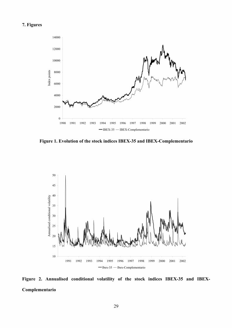
Figure 1 displays the weekly evolution of the stock indices IBEX-35 and IBEX-Complementario in

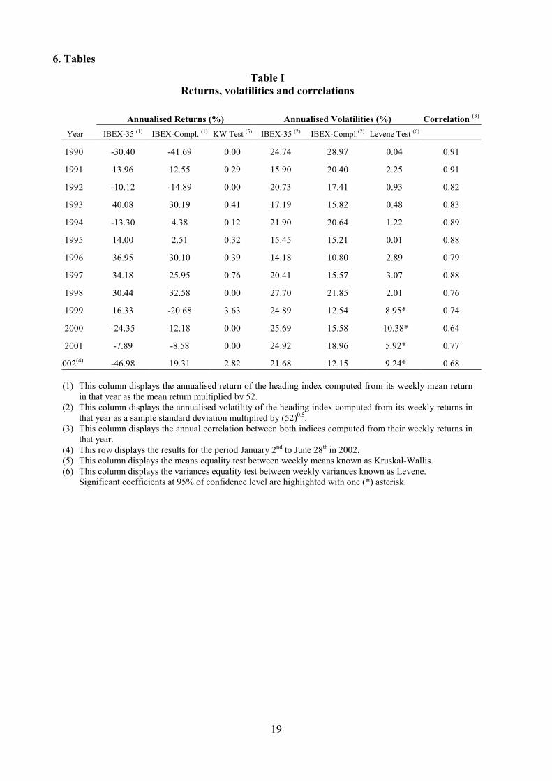
the studied period and preliminary data analysis is presented in Tables I, II and III. Table I displays

returns, volatilities and correlation coefficients, year by year through the sample period for both

stock indices, the IBEX-35 (It) and the IBEX-Complementario (Ct). Three facts can be highlighted

from this table. First, there are 4 years (1994, 1999, 2000 and 2002) in which both indices offer a

different sign return but means equality hypothesis can not be rejected. A second appealing fact in

Table I is that after 1992 the IBEX-35 volatility is fairly larger than the IBEX-Complementario

volatility. Variance equality test rejects the null in years 1999 to 2002. Finally, last column shows

that the correlation between both series has decreased as time pass.

Differences in means and variances can be understood as both classes of stocks offering different

sensitivities to risk factors. For example, large companies are more internationalised depending on

global risk factors and small companies risk factors are localised basically in its own economy. This

fact can be seen as a globalisation effect on the Spanish stock market through several global crises

(European Monetary System suffered several crises in the early nineties, Asian crisis in October

1997,…), international strategic positions taken by the most important Spanish companies

(especially in Latin America) and, simultaneously, these companies have begun to be traded in the

most important stock markets in the world.

5 During the studied period, the IBEX-35 and IBEX-Complementario represented the 82% and the 6%, respectively, of

the overall capitalisation of the Spanish Stock Exchange.

6 The common tests of unit roots and cointegration (Dickey and Fuller (1981), Phillips and Perron (1988), and Johansen

(1988)) offered no doubt about this point.

10

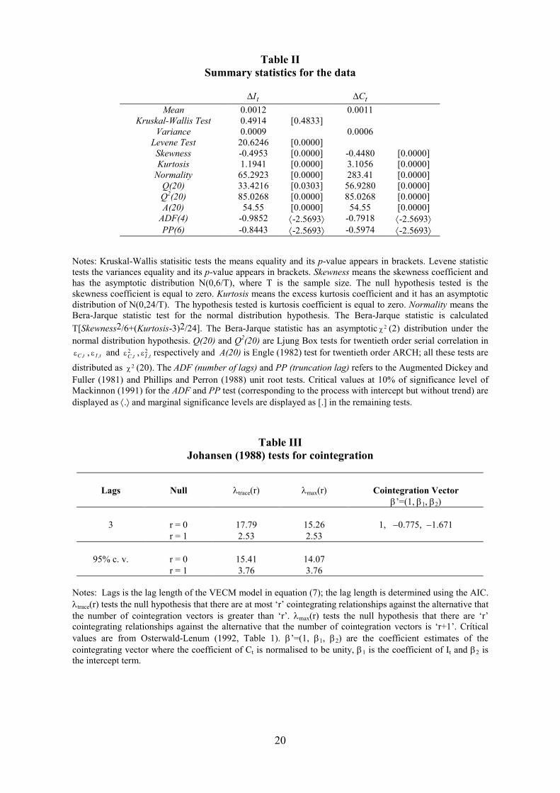
From Table II, it can be stated that the pair of financial time series used in this paper offers very

similar statistics. Both have significant skewness, kurtosis, autocorrelation, heteroskedasticity and a

single unit root. Moreover, although equality in means can not be rejected the variances equality

test is rejected. This preliminary result points out that more research is necessary in the covariance

dynamics between both financial time series.

3.3. Estimating the Model

The model in equations (1) and (3) is estimated in a two-step procedure. To take account of the pre-

holiday effect on the Spanish Stock Exchange7, a dummy variable has been also included in the

mean equation. The model for the means is:

∑∑

∑∑

=−

=−−

=−

=−−

+∆+∆+++=∆

+∆+∆+++=∆

p

jt,jtj,

p

jjtj,ttt

p

jt,jtj,

p

jjtj,ttt

CbIaHOLdzcC

CbIaHOLdzcI

122

122122

111

111111

εα

εα

(7)

where HOLt is a dummy variable that equals to one when the next weekly return contains a pre-

holiday.

First, the VECM model in equation (7) is estimated by Ordinary Least Squares applied equation by

equation (see Engle and Granger (1987)). The VECM lag was chosen by maximising AIC criterion.

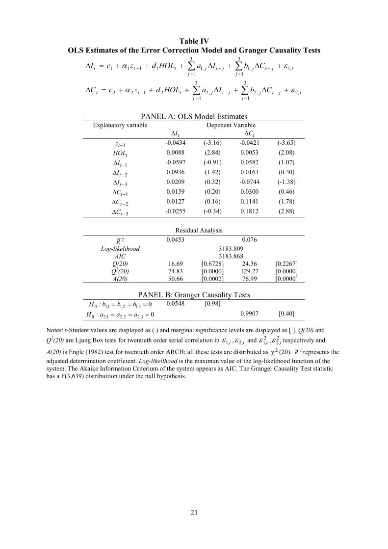
Table III shows that series are cointegrated being 3 the optimum lag length. Panel (A) in Table IV

displays the estimated coefficients and the residual analysis.

Examination of the speed of adjustment coefficients (α1 and α2) provides insight into the

adjustment process of stock indices towards the long-run equilibrium. For the stock indices to adjust

to the long-run relationship it is necessary that α1 > 0 and α2 < 0 (assuming IBEX-35 to be weak

7 See Meneu and Pardo (2003).

11

exogenous and IBEX-Complementario endogenous) 8. The estimated coefficients have the expected

sign in the IBEX-Complementario (α2 ) equation but it has the opposite sign in the IBEX equation

(α1 ). It can be conclude that the IBEX-35 leads the IBEX-Complementario in the long run.

From Table IV, it can be seen that the pre-holiday dummy coefficients are significant in both

equations. This variable has already been studied in Meneu and Pardo (2003) with daily series, but

it is the first time that it is found significant in weekly series. So it can be inferred that it is a very

important anomaly and it should not be omitted.

The residual analysis in Table IV shows that with the estimated model autocorrelation disappears

but heteroskedasticity remains. Furthermore, in Panel (B) Granger causality tests reject the null

hypothesis. Therefore, there is no causality in any sense in the short run.

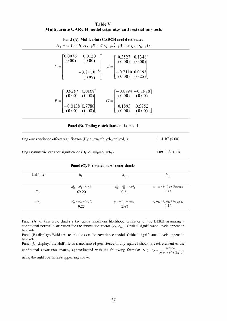
Table V and VI display the estimated conditional covariance model and its standardised residual

analysis, respectively. Table V estimates have been computed assuming a conditional normal

distribution for the innovation vector (ε1t,ε2t)’. The standard errors and their associated critical

significance levels are calculated using the quasi-maximum likelihood method of Bollerslev and

Wooldridge (1992) which are robust to the non-normality assumption. Panel (A) displays the

estimates. The low critical significance level obtained for 13 out of 15 parameter estimates reveals

that this model fit very well with the data.9 Restrictions on cross-variance effects and asymmetric

covariance are clearly rejected (see Panel (B)). As a consequence, cross relationships across all

conditional moments and their shocks (symmetric and non-symmetric) cannot be skipped.

Moreover, asymmetries but it self are also significant. Panel (C) shows the estimated persistence to

any shock in the estimated conditional covariance model. The conditional variance for the IBEX-35

has a very high persistence to its own shock. But volatility persistence is a quite common feature in

financial time series.

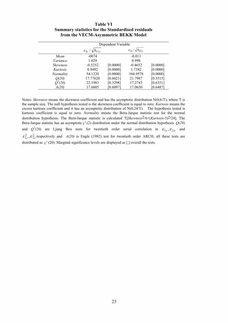
Table VI displays standardised residual analysis. From this table it can be concluded that

autocorrelation and heteroskedasticity problems have been successfully amended. Finally, Figure 2

displays the conditional second moments evolution overall the estimation period. Both volatility

8 From the cointegration relationship, the error correction term can be written as tttt ICz 21 ββ −−= . For the

existence of a long-run equilibrium relationship, it is necessary that 011 >−tzα and 012 <−tzα . See Johansen (1995),

chapter 8 for more details.

9 The maximum log-likelihood function value obtained in the estimation process was 4460.

12

series have similar patterns but Ibex-35 volatility is almost ever above of the Ibex-Complementario

volatility, especially after 1997 when the globalisation effect on the biggest companies in the IBEX-

35 is particularly important.

3.4. Filtering Covariance Asymmetries

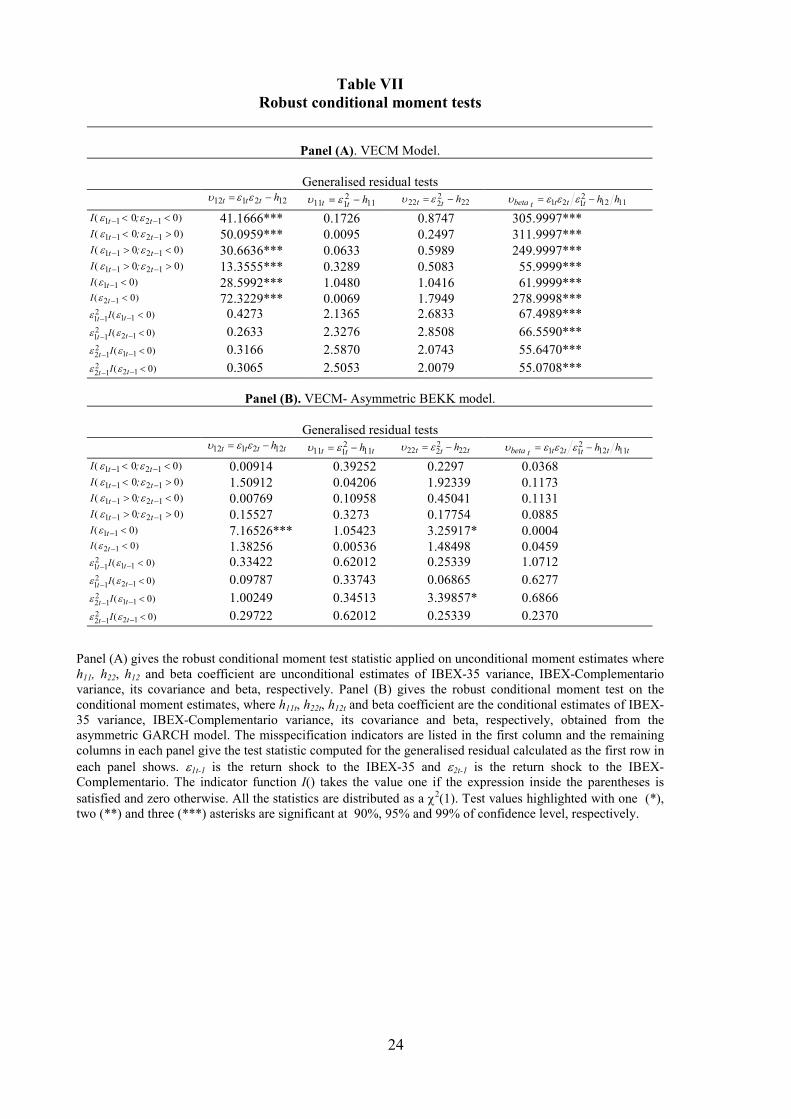
Table VII contains the results of the robust conditional moment of Wooldridge (1990) to test how

the Asymmetric BEKK-GARCH model cleans up the asymmetries in the conditional covariance

matrix. Panel (A) displays the test result when unconditional covariance estimate is used. It can be

seen than asymmetries are very important, especially in the covariance between both series and beta

coefficients. Panel (B) offers the test results once asymmetries are included in the covariance

specification. After this, only one asymmetric pattern seems to remain in the conditional covariance

specification. This is an important result because it means that the GARCH specification is

gathering almost all the possible asymmetries in the conditional covariance matrix: direct and

crossed asymmetries and asymmetries of sign and size in the unexpected shocks. This result is also

a guarantee that the analysis of the asymmetric volatility impulse response function carried out later

is reliable. That is, it will be able to answer the following questions: Are spillovers of volatility

important in the large-small firm system? Are the unexpected negative shocks of large stocks

conditional variance important in the small stocks conditional covariance? And the reverse? Which

market leads the volatility system?

The effect of asymmetric behaviour in conditional beta coefficients is also investigated. Last

column in Table VII contains its robust conditional moment test10. The presence of any asymmetric

effect is clearly rejected in Panel (B). This result shows that conditional beta estimates are

insensitive to volatility asymmetries. This appealing result comes from the fact that a ratio between

two second moments tends to compensate the asymmetric effect if a stable proportion is maintained

between both conditional second moments. This lack of sensitivity is important for portfolio

management based on beta estimates, as it seems unnecessary to consider asymmetries11, therefore

simpler models can be used. It is also important because beta coefficients are a market risk

10 Following Wooldridge (1990), a consistent estimator of the minimum variance hedge ratio is built using the

continuous function property on consistent estimators (see Hamilton (1994), p. 182).

11 Results on symmetric BEKK model show that conditional beta estimates are insensitive to any asymmetry in the

conditional covariance matrix. Results are omitted to conserve space.

13

sensitivity measure and it is shown that conditional beta estimates are insensitive to sign and size

shocks. Furthermore, this result is comparable to the Braun et al. (1995) and Bekaert and Wu

(2000) empirical findings on beta coefficients: while asymmetries are very strong in the conditional

second moments they appear to be entirely absent in conditional betas.

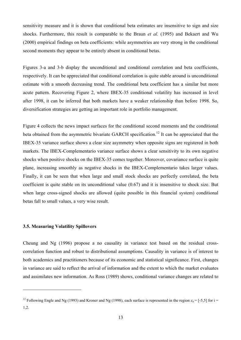
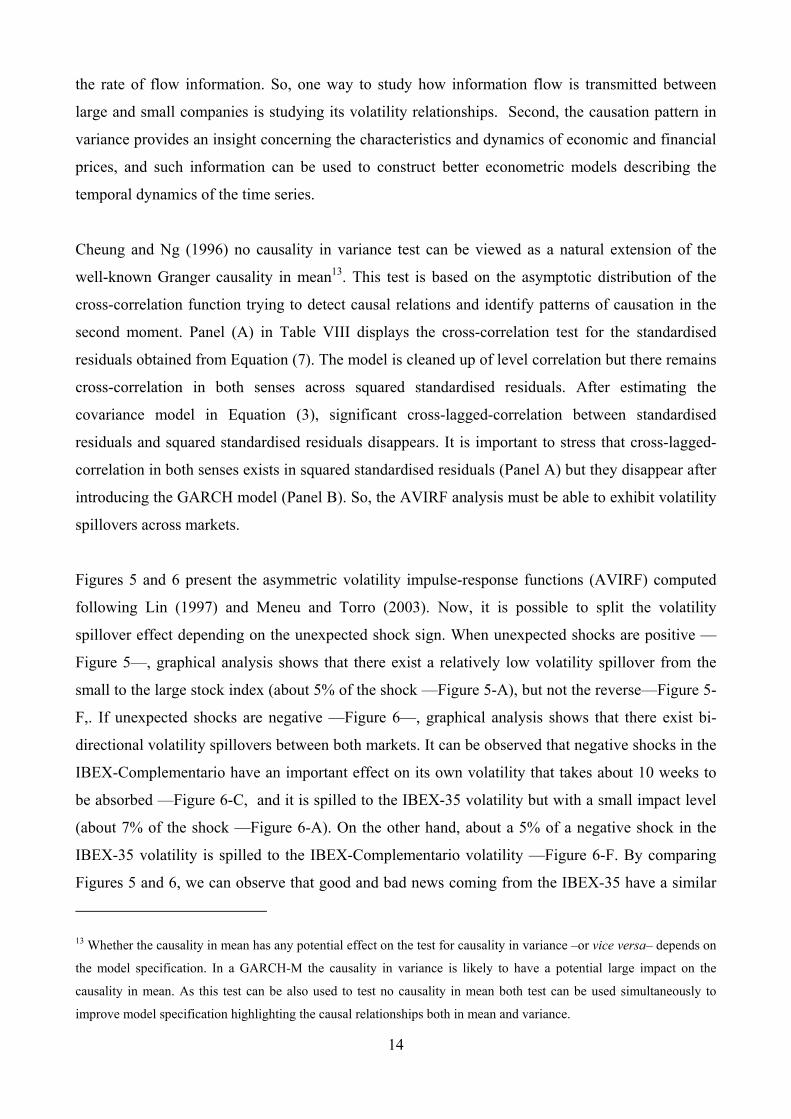
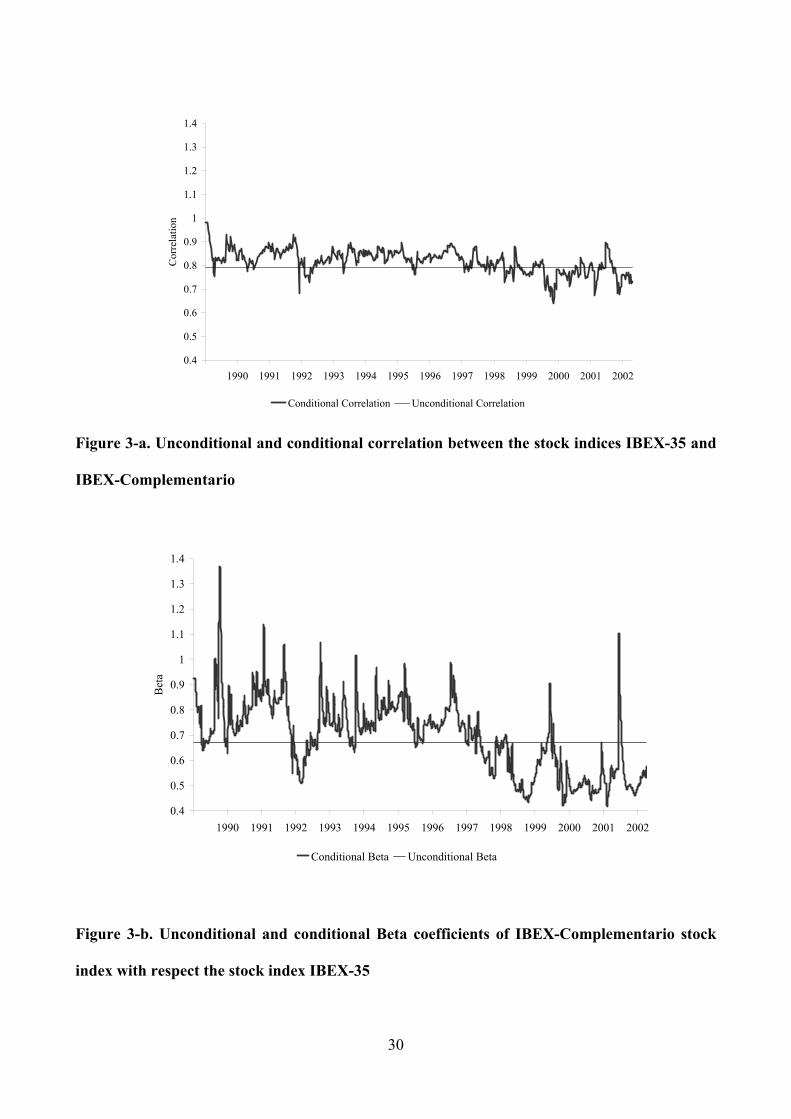
Figures 3-a and 3-b display the unconditional and conditional correlation and beta coefficients,

respectively. It can be appreciated that conditional correlation is quite stable around is unconditional

estimate with a smooth decreasing trend. The conditional beta coefficient has a similar but more

acute pattern. Recovering Figure 2, where IBEX-35 conditional volatility has increased in level

after 1998, it can be inferred that both markets have a weaker relationship than before 1998. So,

diversification strategies are getting an important role in portfolio management.

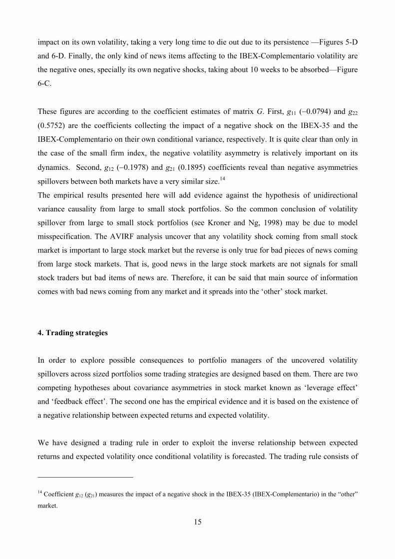
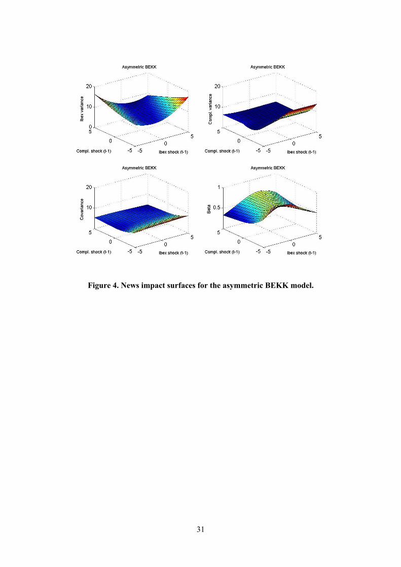
Figure 4 collects the news impact surfaces for the conditional second moments and the conditional

beta obtained from the asymmetric bivariate GARCH specification.12 It can be appreciated that the

IBEX-35 variance surface shows a clear size asymmetry when opposite signs are registered in both

markets. The IBEX-Complementario variance surface shows a clear sensitivity to its own negative

shocks when positive shocks on the IBEX-35 comes together. Moreover, covariance surface is quite

plane, increasing smoothly as negative shocks in the IBEX-Complementario takes larger values.

Finally, it can be seen that when large and small stock shocks are perfectly correlated, the beta

coefficient is quite stable on its unconditional value (0.67) and it is insensitive to shock size. But

when large cross-signed shocks are allowed (quite possible in this financial system) conditional

betas fall to small values, a very wise result.

3.5. Measuring Volatility Spillovers

Cheung and Ng (1996) propose a no causality in variance test based on the residual cross-

correlation function and robust to distributional assumptions. Causality in variance is of interest to

both academics and practitioners because of its economic and statistical significance. First, changes

in variance are said to reflect the arrival of information and the extent to which the market evaluates

and assimilates new information. As Ross (1989) shows, conditional variance changes are related to

12 Following Engle and Ng (1993) and Kroner and Ng (1998), each surface is represented in the region εit = [-5,5] for i =

1,2.

14

the rate of flow information. So, one way to study how information flow is transmitted between

large and small companies is studying its volatility relationships. Second, the causation pattern in

variance provides an insight concerning the characteristics and dynamics of economic and financial

prices, and such information can be used to construct better econometric models describing the

temporal dynamics of the time series.

Cheung and Ng (1996) no causality in variance test can be viewed as a natural extension of the

well-known Granger causality in mean13. This test is based on the asymptotic distribution of the

cross-correlation function trying to detect causal relations and identify patterns of causation in the

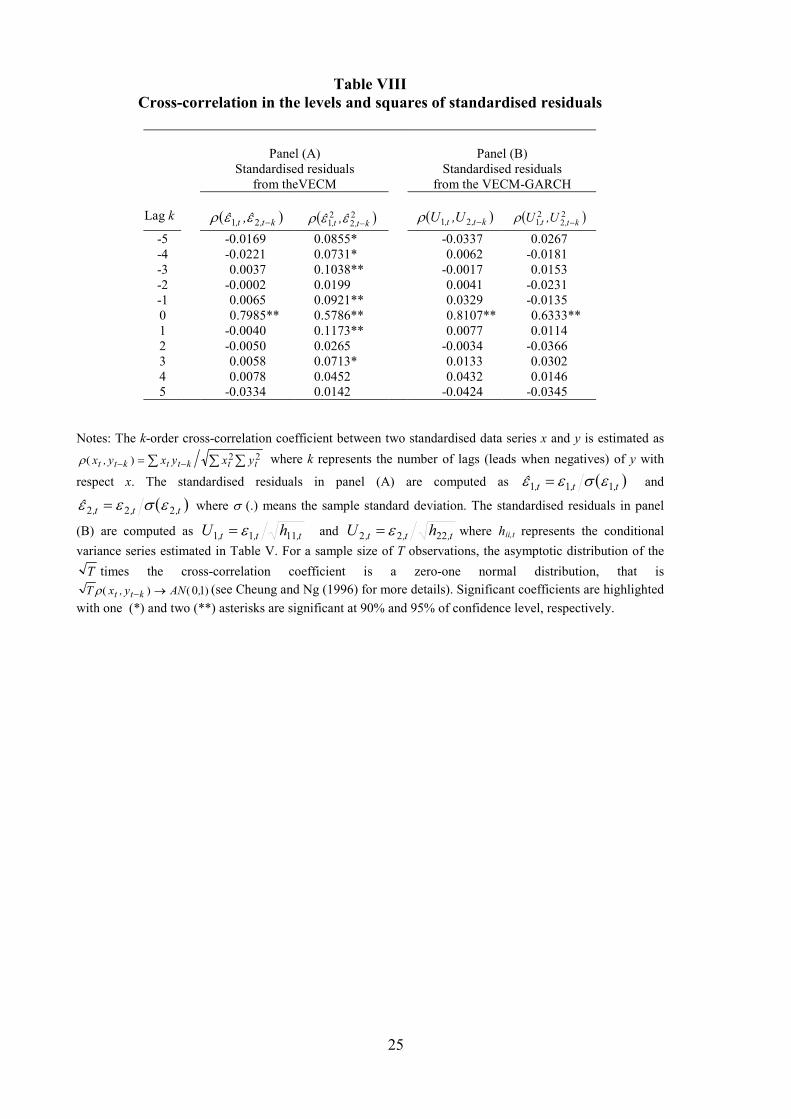
second moment. Panel (A) in Table VIII displays the cross-correlation test for the standardised

residuals obtained from Equation (7). The model is cleaned up of level correlation but there remains

cross-correlation in both senses across squared standardised residuals. After estimating the

covariance model in Equation (3), significant cross-lagged-correlation between standardised

residuals and squared standardised residuals disappears. It is important to stress that cross-lagged-

correlation in both senses exists in squared standardised residuals (Panel A) but they disappear after

introducing the GARCH model (Panel B). So, the AVIRF analysis must be able to exhibit volatility

spillovers across markets.

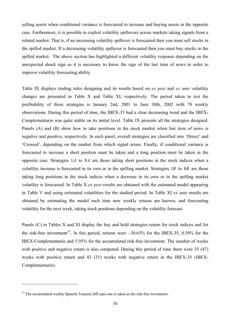
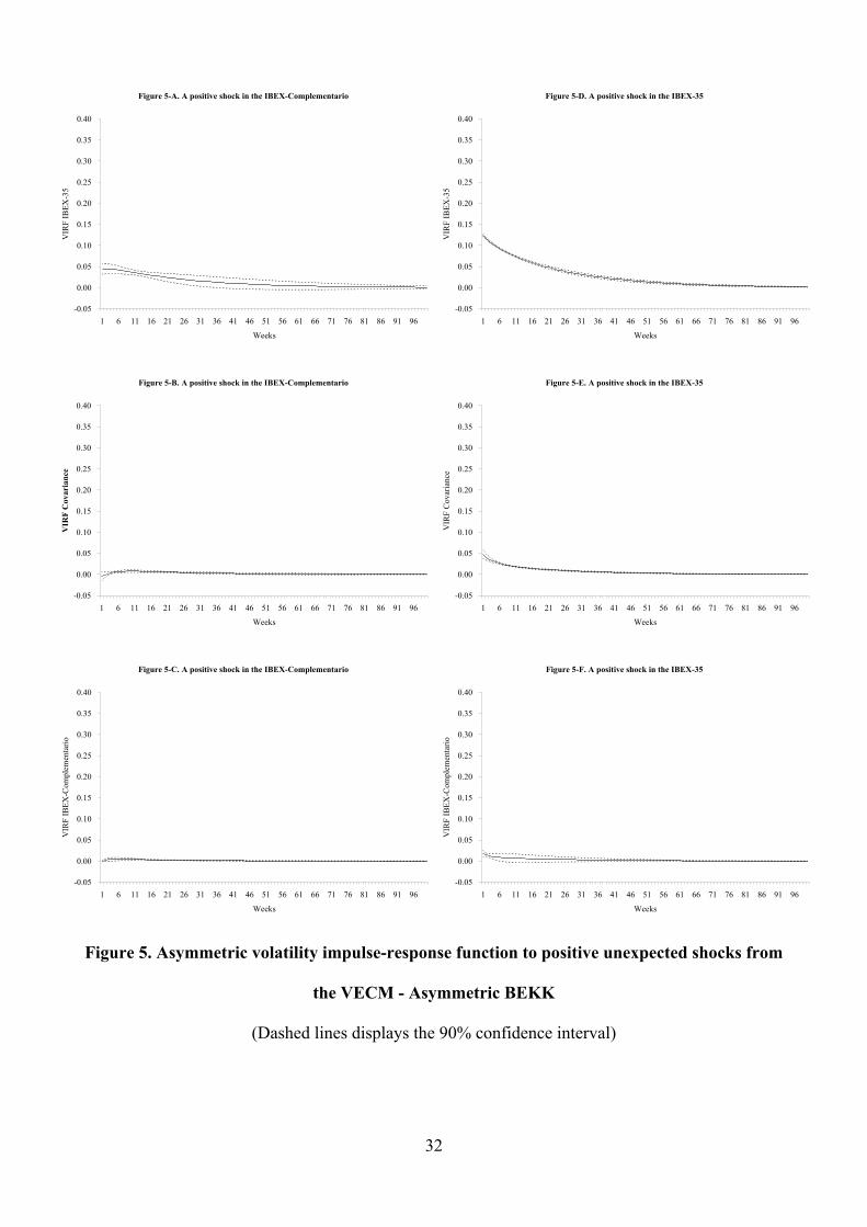
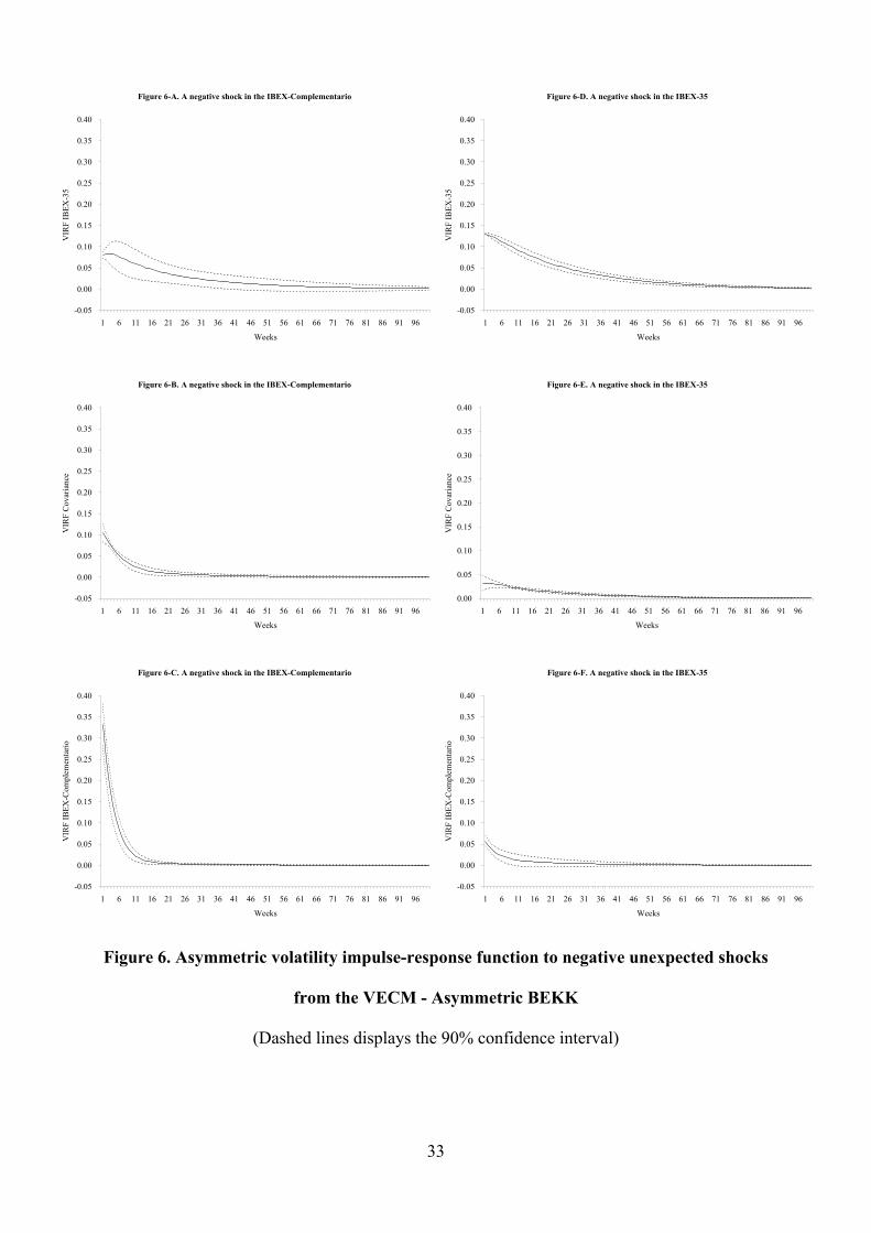
Figures 5 and 6 present the asymmetric volatility impulse-response functions (AVIRF) computed

following Lin (1997) and Meneu and Torro (2003). Now, it is possible to split the volatility

spillover effect depending on the unexpected shock sign. When unexpected shocks are positive —

Figure 5—, graphical analysis shows that there exist a relatively low volatility spillover from the

small to the large stock index (about 5% of the shock —Figure 5-A), but not the reverse—Figure 5-

F,. If unexpected shocks are negative —Figure 6—, graphical analysis shows that there exist bi-

directional volatility spillovers between both markets. It can be observed that negative shocks in the

IBEX-Complementario have an important effect on its own volatility that takes about 10 weeks to

be absorbed —Figure 6-C, and it is spilled to the IBEX-35 volatility but with a small impact level

(about 7% of the shock —Figure 6-A). On the other hand, about a 5% of a negative shock in the

IBEX-35 volatility is spilled to the IBEX-Complementario volatility —Figure 6-F. By comparing

Figures 5 and 6, we can observe that good and bad news coming from the IBEX-35 have a similar

13 Whether the causality in mean has any potential effect on the test for causality in variance –or vice versa– depends on

the model specification. In a GARCH-M the causality in variance is likely to have a potential large impact on the

causality in mean. As this test can be also used to test no causality in mean both test can be used simultaneously to

improve model specification highlighting the causal relationships both in mean and variance.

15

impact on its own volatility, taking a very long time to die out due to its persistence —Figures 5-D

and 6-D. Finally, the only kind of news items affecting to the IBEX-Complementario volatility are

the negative ones, specially its own negative shocks, taking about 10 weeks to be absorbed—Figure

6-C.

These figures are according to the coefficient estimates of matrix G. First, g11 (−0.0794) and g22

(0.5752) are the coefficients collecting the impact of a negative shock on the IBEX-35 and the

IBEX-Complementario on their own conditional variance, respectively. It is quite clear than only in

the case of the small firm index, the negative volatility asymmetry is relatively important on its

dynamics. Second, g12 (−0.1978) and g21 (0.1895) coefficients reveal than negative asymmetries

spillovers between both markets have a very similar size.14

The empirical results presented here will add evidence against the hypothesis of unidirectional

variance causality from large to small stock portfolios. So the common conclusion of volatility

spillover from large to small stock portfolios (see Kroner and Ng, 1998) may be due to model

misspecification. The AVIRF analysis uncover that any volatility shock coming from small stock

market is important to large stock market but the reverse is only true for bad pieces of news coming

from large stock markets. That is, good news in the large stock markets are not signals for small

stock traders but bad items of news are. Therefore, it can be said that main source of information

comes with bad news coming from any market and it spreads into the ‘other’ stock market.

4. Trading strategies

In order to explore possible consequences to portfolio managers of the uncovered volatility

spillovers across sized portfolios some trading strategies are designed based on them. There are two

competing hypotheses about covariance asymmetries in stock market known as ‘leverage effect’

and ‘feedback effect’. The second one has the empirical evidence and it is based on the existence of

a negative relationship between expected returns and expected volatility.

We have designed a trading rule in order to exploit the inverse relationship between expected

returns and expected volatility once conditional volatility is forecasted. The trading rule consists of

14 Coefficient g12 (g21) measures the impact of a negative shock in the IBEX-35 (IBEX-Complementario) in the “other”

market.

16

selling assets when conditional variance is forecasted to increase and buying assets in the opposite

case. Furthermore, it is possible to exploit volatility spillovers across markets taking signals from a

related market. That is, if an increasing volatility spillover is forecasted then you must sell stocks in

the spilled market. If a decreasing volatility spillover is forecasted then you must buy stocks in the

spilled market. The above section has highlighted a different volatility response depending on the

unexpected shock sign so it is necessary to know the sign of the last item of news in order to

improve volatility forecasting ability.

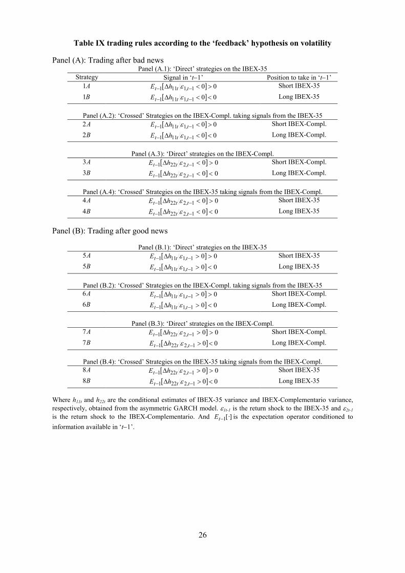
Table IX displays trading rules designing and its results based on ex post and ex ante volatility

changes are presented in Table X and Table XI, respectively. The period taken to test the

profitability of these strategies is January 2nd, 2001 to June 30th, 2002 with 78 weekly

observations. During this period of time, the IBEX-35 had a clear decreasing trend and the IBEX-

Complementario was quite stable on its initial level. Table IX presents all the strategies designed.

Panels (A) and (B) show how to take positions in the stock market when last item of news is

negative and positive, respectively. In each panel, overall strategies are classified into ‘Direct’ and

‘Crossed’, depending on the market from which signal arises. Finally, if conditional variance is

forecasted to increase a short position must be taken and a long position must be taken in the

opposite case. Strategies A1 to A8 are those taking short positions in the stock indices when a

volatility increase is forecasted in its own or in the spilling market. Strategies B1 to B8 are those

taking long positions in the stock indices when a decrease in its own or in the spilling market

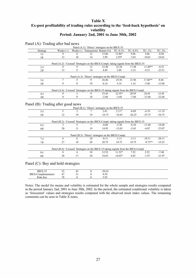
volatility is forecasted. In Table X ex post results are obtained with the estimated model appearing

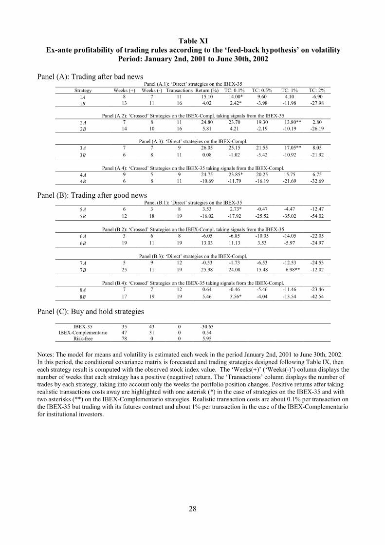
in Table V and using estimated volatilities for the studied period. In Table XI ex ante results are

obtained by estimating the model each time new weekly returns are known, and forecasting

volatility for the next week, taking stock positions depending on the volatility forecast.

Panels (C) in Tables X and XI display the buy and hold strategies return for stock indices and for

the risk-free investment15. In this period, returns were −30.63% for the IBEX-35, 0.54% for the

IBEX-Complementario and 5.95% for the accumulated risk-free investment. The number of weeks

with positive and negative return is also computed. During this period of time there were 35 (47)

weeks with positive return and 43 (31) weeks with negative return in the IBEX-35 (IBEX-

Complementario).

15 The accumulated weekly Spanish Treasury bill repo rate is taken as the risk-free investment.

17

Before considering profitable a trading rule, transaction cost must be considered. Approximately,

institutional investors trading on the IBEX-35 will require no more than a 0.5% expenses in

transactions costs (commissions, spreads, …). The IBEX-Complementario will require no more

than 1%. Finally, if the futures contract on the IBEX-35 is used instead of the spot index, no more

than 0.1% expenses will be required. Results on the futures contract are not displayed but are

virtually identical to the spot index using the first to delivery contract. So the viable strategies are

those than have a positive return after considering transaction costs of 0.1% in the IBEX-35 based

strategies and 1% in the IBEX-Complementario case.

Tables X and XI show similar results. There only exists one strategy that is profitable ex post but it

is no profitable in the ex ante case, the strategy A8 . All the remaining strategies identified as

profitable or non-profitable agree in both tables16. Hence, the following comments refer to both

tables but after excluding this strategy. Profitable strategies are marked with an asterisk in the case

of positions taken in the IBEX-35 and with two asterisks in the case of the IBEX-Complementario

positions. The profitable strategies are the following: A1 , A2 , A3 , A4 , A5 , B1 , B7 and B8 .

From net returns it is easy to see that the four strategies involving short positions after bad news

( A1 , A2 , A3 and A4 ) have the better performance. So one can conclude that when an increase in

volatility is forecasted after bad news, then a short position must be taken in the stock market. It is

important to stress that strategies based on signals coming from the neighbour market ( A2 and A4 )

are very profitable. It is important to point out that this is a decreasing period for the IBEX-35 and

selling rules will tend to have positive returns. However, this is not true for the IBEX-

Complementario (see Figure 1). It should be remembered that there are 43 out of 78 weeks with

negative return in the IBEX-35, but there are only 31 in the IBEX-Complementario. Therefore, this

is not a hazardous result.

The four strategies with better performance ( A1 , A2 , A3 and A4 ) involve taking short positions in

the stock market. For large financial institutions is possible to take short positions in both the small

and large stock index. In concrete, taking short positions in the IBEX-35 is very easy to any

investor by joining its futures market. So one can conclude that profitable strategies have existed in

the studied period of time.

16 If a risk-free investment position were taken each non-trading week, it should be added at least a 3% of extra return.

18

5. Summary and conclusions

In this article we study the dynamic relationships between large and small firms taking into account

asymmetric volatility and covariance asymmetry. When these types of structures appear, it is

necessary to distinguish between positive and negative shocks. The Volatility Impulse-Response

Functions proposed by Lin (1997) and extended by Meneu and Torró (2003) become especially

useful in this case, since they give information on the second moment interaction between related

markets, and they allow practitioners to design trading rules based on the inverse relationship

existing between expected volatilities and expected returns.

The main result is that there exist volatility spillovers across sized portfolios in both senses after bad

pieces of news. Therefore, bad news about large firms can cause volatility in both large-firm returns

and small-firm returns but bad news about small firms can also cause volatility in both kind of

firms. Ross (1989) demonstrated that variance changes are related to the rate of information flow.

Our results indicate that only bad piece of news contains information, no matter the size of the firm.

After measuring spillover effects, different trading rules have been designed. Specifically, a trading

rule taking advantage of this empirical supported feature is selling assets when conditional variance

is forecasted to increase and buying assets in the opposite case. Furthermore, it is possible to exploit

volatility spillovers across markets taking signals from a related market. Results show that very

profitable strategies exist, especially after bad news coming from its own and the ‘other’ market.

Whether this result is against rational market hypothesis or it can be explained by time-varying risk-

premiums overcomes the objectives of this paper and it is left for further research.

19

6. Tables

Table IReturns, volatilities and correlations

Annualised Returns (%) Annualised Volatilities (%) Correlation (3)

Year IBEX-35 (1) IBEX-Compl. (1) KW Test (5) IBEX-35 (2) IBEX-Compl.(2) Levene Test (6)

1990 -30.40 -41.69 0.00 24.74 28.97 0.04 0.91

1991 13.96 12.55 0.29 15.90 20.40 2.25 0.91

1992 -10.12 -14.89 0.00 20.73 17.41 0.93 0.82

1993 40.08 30.19 0.41 17.19 15.82 0.48 0.83

1994 -13.30 4.38 0.12 21.90 20.64 1.22 0.89

1995 14.00 2.51 0.32 15.45 15.21 0.01 0.88

1996 36.95 30.10 0.39 14.18 10.80 2.89 0.79

1997 34.18 25.95 0.76 20.41 15.57 3.07 0.88

1998 30.44 32.58 0.00 27.70 21.85 2.01 0.76

1999 16.33 -20.68 3.63 24.89 12.54 8.95* 0.74

2000 -24.35 12.18 0.00 25.69 15.58 10.38* 0.64

2001 -7.89 -8.58 0.00 24.92 18.96 5.92* 0.77

2002(4) -46.98 19.31 2.82 21.68 12.15 9.24* 0.68

(1) This column displays the annualised return of the heading index computed from its weekly mean returnin that year as the mean return multiplied by 52.

(2) This column displays the annualised volatility of the heading index computed from its weekly returns inthat year as a sample standard deviation multiplied by (52)0.5.

(3) This column displays the annual correlation between both indices computed from their weekly returns inthat year.

(4) This row displays the results for the period January 2nd to June 28th in 2002.(5) This column displays the means equality test between weekly means known as Kruskal-Wallis.(6) This column displays the variances equality test between weekly variances known as Levene.

Significant coefficients at 95% of confidence level are highlighted with one (*) asterisk.

20

Table IISummary statistics for the data

tI∆ tC∆Mean 0.0012 0.0011

Kruskal-Wallis Test 0.4914 [0.4833]Variance 0.0009 0.0006

Levene Test 20.6246 [0.0000]Skewness -0.4953 [0.0000] -0.4480 [0.0000]Kurtosis 1.1941 [0.0000] 3.1056 [0.0000]

Normality 65.2923 [0.0000] 283.41 [0.0000]Q(20) 33.4216 [0.0303] 56.9280 [0.0000]Q2(20) 85.0268 [0.0000] 85.0268 [0.0000]A(20) 54.55 [0.0000] 54.55 [0.0000]

ADF(4) -0.9852 ⟨-2.5693⟩ -0.7918 ⟨-2.5693⟩PP(6) -0.8443 ⟨-2.5693⟩ -0.5974 ⟨-2.5693⟩

Notes: Kruskal-Wallis statisitic tests the means equality and its p-value appears in brackets. Levene statistictests the variances equality and its p-value appears in brackets. Skewness means the skewness coefficient andhas the asymptotic distribution N(0,6/T), where T is the sample size. The null hypothesis tested is theskewness coefficient is equal to zero. Kurtosis means the excess kurtosis coefficient and it has an asymptoticdistribution of N(0,24/T). The hypothesis tested is kurtosis coefficient is equal to zero. Normality means theBera-Jarque statistic test for the normal distribution hypothesis. The Bera-Jarque statistic is calculatedT[Skewness2/6+(Kurtosis-3)2/24]. The Bera-Jarque statistic has an asymptotic 2χ (2) distribution under thenormal distribution hypothesis. Q(20) and Q2(20) are Ljung Box tests for twentieth order serial correlation in

t,Cε , t,Iε and 2t,Cε , 2

t,Iε respectively and A(20) is Engle (1982) test for twentieth order ARCH; all these tests aredistributed as 2χ (20). The ADF (number of lags) and PP (truncation lag) refers to the Augmented Dickey andFuller (1981) and Phillips and Perron (1988) unit root tests. Critical values at 10% of significance level ofMackinnon (1991) for the ADF and PP test (corresponding to the process with intercept but without trend) aredisplayed as ⟨.⟩ and marginal significance levels are displayed as [.] in the remaining tests.

Table IIIJohansen (1988) tests for cointegration

Lags Null λtrace(r) λmax(r) Cointegration Vectorβ’=(1, β1, β2)

3 r = 0r = 1

17.792.53

15.262.53

1, −0.775, −1.671

95% c. v. r = 0r = 1

15.413.76

14.073.76

Notes: Lags is the lag length of the VECM model in equation (7); the lag length is determined using the AIC.λtrace(r) tests the null hypothesis that there are at most ‘r’ cointegrating relationships against the alternative thatthe number of cointegration vectors is greater than ‘r’. λmax(r) tests the null hypothesis that there are ‘r’cointegrating relationships against the alternative that the number of cointegration vectors is ‘r+1’. Críticalvalues are from Osterwald-Lenum (1992, Table 1). β’=(1, β1, β2) are the coefficient estimates of thecointegrating vector where the coefficient of Ct is normalised to be unity, β1 is the coefficient of It and β2 isthe intercept term.

21

Table IVOLS Estimates of the Error Correction Model and Granger Causality Tests

∑∑

∑∑

=−

=−−

=−

=−−

+∆+∆+++=∆

+∆+∆+++=∆

3

122

3

122122

3

111

3

111111

jt,jtj,

jjtj,ttt

jt,jtj,

jjtj,ttt

CbIaHOLdzcC

CbIaHOLdzcI

εα

εα

PANEL A: OLS Model EstimatesExplanatory variable Depenent Variable

tI∆ tC∆

1−tz -0.0434 (-3.16) -0.0421 (-3.65)

tHOL 0.0088 (2.84) 0.0053 (2.08)

1−∆ tI -0.0597 (-0.91) 0.0582 (1.07)

2−∆ tI 0.0936 (1.42) 0.0163 (0.30)

3−∆ tI 0.0209 (0.32) -0.0744 (-1.38)

1−∆ tC 0.0159 (0.20) 0.0300 (0.46)

2−∆ tC 0.0127 (0.16) 0.1141 (1.78)

3−∆ tC -0.0255 (-0.34) 0.1812 (2.88)

Residual Analysis2R 0.0453 0.076

Log-likelihood 3183.809AIC 3183.868

Q(20) 16.69 [0.6728] 24.36 [0.2267]Q2(20) 74.83 [0.0000] 129.27 [0.0000]A(20) 50.66 [0.0002] 76.99 [0.0000]

PANEL B: Granger Causality Tests03121110 === ,,, bbb:H 0.0548 [0.98]

03222120 === ,,, aaa:H 0.9907 [0.40]

Notes: t-Student values are displayed as (.) and marginal significance levels are displayed as [.]. Q(20) andQ2(20) are Ljung Box tests for twentieth order serial correlation in t,1ε , t,2ε and 2

1 t,ε , 22 t,ε respectively and

A(20) is Engle (1982) test for twentieth order ARCH; all these tests are distributed as 2χ (20). 2R represents theadjusted determination coefficient. Log-likelihood is the maximun value of the log-likelihood function of thesystem. The Akaike Information Criterium of the system appears as AIC. The Granger Causality Test statistichas a F(3,639) distribuition under the null hypothesis.

22

Table V Multivariate GARCH model estimates and restrictions tests

Panel (A). Multivariate GARCH model estimatesG'GA'ABH'BC'CH '

tt'tttt 11111 −−−−− +++= ηηεε

( ) ( )

( )

( ) ( )

( ) ( )

( ) ( )

( ) ( )

( ) ( )

( ) ( )

−−

=

−=

−=

×−=

−

0000005752018950

0000001978007940

0000007788001380

0000000168092870

2500000198021100

0000001348035270

9901083

0000000120000760

8

....

....

G

....

....

B

....

....

A

..

....

C

Panel (B). Testing restrictions on the model

sting cross-variance effects significance (H0: a12=a21=b12=b21=d12=d21). 1.61 106 (0.00)

sting asymmetric variance significance (H0: d11=d12=d21=d22). 1.09 103 (0.00)

Panel (C). Estimated persistence shocks

Half life 11h 22h 12h

t,1ε211

211

211 ½gba ++

69.20

212

212

212 ½gba ++

0.21111211121112 ¼ ggbbaa ++

0.43

t,2ε 221

221

221 ½gba ++

0.25

222

222

222 ½gba ++

2.68222122212221 ¼ ggbbaa ++

0.16

Panel (A) of this table displays the quasi maximum likelihood estimates of the BEKK assuming aconditional normal distribution for the innovation vector (ε1τ.ε2τ)’. Critical significance levels appear inbrackets.Panel (B) displays Wald test restrictions on the covariance model. Critical significance levels appear inbrackets.Panel (C) displays the Half-life as a measure of persistence of any squared shock in each element of the

conditional covariance matrix, approximated with the following formula: )gbaln(

).ln(lifeHalf 222 ½50++

=− ,

using the right coefficients appearing above.

23

Table VISummary statistics for the Standardised residuals

from the VECM-Asymmetric BEKK Model

Dependent Variable

t,t h/ 111ε t,t h/ 222ε

Mean -0074 -0.011Variance 1.029 0.998Skewness -0.5252 [0.0000] -0.4652 [0.0000]Kurtosis 0.9492 [0.0000] 1.7382 [0.0000]

Normality 54.1220 [0.0000] 104.9578 [0.0000]Q(20) 17.77620 [0.6021] 21.7987 [0.3515]Q2(20) 22.1983 [0.3298] 17.2743 [0.6351]A(20) 17.6605 [0.6097] 17.0650 [0.6487]

Notes: Skewness means the skewness coefficient and has the asymptotic distribution N(0;6/T), where T isthe sample size. The null hypothesis tested is the skewness coefficient is equal to zero. Kurtosis means theexcess kurtosis coefficient and it has an asymptotic distribution of N(0,24/T). The hypothesis tested iskurtosis coefficient is equal to zero. Normality means the Bera-Jarque statistic test for the normaldistribution hypothesis. The Bera-Jarque statistic is calculated T[Skewness2/6+(Kurtosis-3)2/24]. TheBera-Jarque statistic has an asymptotic 2χ (2) distribution under the normal distribution hypothesis. Q(20)and Q2(20) are Ljung Box tests for twentieth order serial correlation in t,1ε , t,2ε and

21 t,ε , 2

2 t,ε respectively and A(20) is Engle (1982) test for twentieth order ARCH; all these tests aredistributed as 2χ (20). Marginal significance levels are displayed as [.] overall the tests.

24

Table VIIRobust conditional moment tests

Panel (A). VECM Model.

Generalised residual tests122112 httt −= εευ 11

2111 htt −= ευ 22

2222 htt −= ευ 1112

2121 hhttttbeta −= εεευ

( )00 1211 << −− tt ;I εε 41.1666*** 0.1726 0.8747 305.9997***( )00 1211 >< −− tt ;I εε 50.0959*** 0.0095 0.2497 311.9997***( )00 1211 <> −− tt ;I εε 30.6636*** 0.0633 0.5989 249.9997***( )00 1211 >> −− tt ;I εε 13.3555*** 0.3289 0.5083 55.9999***( )011 <−tI ε 28.5992*** 1.0480 1.0416 61.9999***( )012 <−tI ε 72.3229*** 0.0069 1.7949 278.9998***

( )0112

11 <−− tt I εε 0.4273 2.1365 2.6833 67.4989***( )012

211 <−− tt I εε 0.2633 2.3276 2.8508 66.5590***

( )0112

12 <−− tt I εε 0.3166 2.5870 2.0743 55.6470***( )012

212 <−− tt I εε 0.3065 2.5053 2.0079 55.0708***

Panel (B). VECM- Asymmetric BEKK model.

Generalised residual teststttt h122112 −= εευ ttt h11

2111 −= ευ ttt h22

2222 −= ευ ttttttbeta hh 1112

2121 −= εεευ

( )00 1211 << −− tt ;I εε 0.00914 0.39252 0.2297 0.0368( )00 1211 >< −− tt ;I εε 1.50912 0.04206 1.92339 0.1173( )00 1211 <> −− tt ;I εε 0.00769 0.10958 0.45041 0.1131( )00 1211 >> −− tt ;I εε 0.15527 0.3273 0.17754 0.0885( )011 <−tI ε 7.16526*** 1.05423 3.25917* 0.0004( )012 <−tI ε 1.38256 0.00536 1.48498 0.0459

( )0112

11 <−− tt I εε 0.33422 0.62012 0.25339 1.0712( )012

211 <−− tt I εε 0.09787 0.33743 0.06865 0.6277

( )0112

12 <−− tt I εε 1.00249 0.34513 3.39857* 0.6866( )012

212 <−− tt I εε 0.29722 0.62012 0.25339 0.2370

Panel (A) gives the robust conditional moment test statistic applied on unconditional moment estimates whereh11, h22, h12 and beta coefficient are unconditional estimates of IBEX-35 variance, IBEX-Complementariovariance, its covariance and beta, respectively. Panel (B) gives the robust conditional moment test on theconditional moment estimates, where h11t, h22t, h12t and beta coefficient are the conditional estimates of IBEX-35 variance, IBEX-Complementario variance, its covariance and beta, respectively, obtained from theasymmetric GARCH model. The misspecification indicators are listed in the first column and the remainingcolumns in each panel give the test statistic computed for the generalised residual calculated as the first row ineach panel shows. ε1t-1 is the return shock to the IBEX-35 and ε2t-1 is the return shock to the IBEX-Complementario. The indicator function I() takes the value one if the expression inside the parentheses issatisfied and zero otherwise. All the statistics are distributed as a χ2(1). Test values highlighted with one (*),two (**) and three (***) asterisks are significant at 90%, 95% and 99% of confidence level, respectively.

25

Table VIIICross-correlation in the levels and squares of standardised residuals

Panel (A)Standardised residuals

from theVECM

Panel (B)Standardised residuals

from the VECM-GARCH

Lag k ( )kt,t, ˆ,ˆ −21 εερ ( )22

21 kt,t, ˆ,ˆ −εερ ( )kt,t, U,U −21ρ ( )2

221 kt,t, U,U −ρ

-5 -0.0169 0.0855* -0.0337 0.0267-4 -0.0221 0.0731* 0.0062 -0.0181-3 0.0037 0.1038** -0.0017 0.0153-2 -0.0002 0.0199 0.0041 -0.0231-1 0.0065 0.0921** 0.0329 -0.01350 0.7985** 0.5786** 0.8107** 0.6333**1 -0.0040 0.1173** 0.0077 0.01142 -0.0050 0.0265 -0.0034 -0.03663 0.0058 0.0713* 0.0133 0.03024 0.0078 0.0452 0.0432 0.01465 -0.0334 0.0142 -0.0424 -0.0345

Notes: The k-order cross-correlation coefficient between two standardised data series x and y is estimated as( ) ∑∑∑ −− = 22

ttkttktt yxyxy,xρ where k represents the number of lags (leads when negatives) of y with

respect x. The standardised residuals in panel (A) are computed as ( )t,t,t,ˆ 111 εσεε = and

( )t,t,t,ˆ 222 εσεε = where σ (.) means the sample standard deviation. The standardised residuals in panel

(B) are computed as t,t,t, hU 1111 ε= and t,t,t, hU 2222 ε= where hii,t represents the conditionalvariance series estimated in Table V. For a sample size of T observations, the asymptotic distribution of the

T times the cross-correlation coefficient is a zero-one normal distribution, that is( ) ( )10,ANy,xT ktt →−ρ (see Cheung and Ng (1996) for more details). Significant coefficients are highlighted

with one (*) and two (**) asterisks are significant at 90% and 95% of confidence level, respectively.

26

Table IX trading rules according to the ‘feedback’ hypothesis on volatility

Panel (A): Trading after bad newsPanel (A.1): ‘Direct’ strategies on the IBEX-35

Strategy Signal in ‘t−1’ Position to take in ‘t−1’A1 [ ] 0011111 ><∆ −− t,tt hE ε Short IBEX-35

B1 [ ] 0011111 <<∆ −− t,tt hE ε Long IBEX-35

Panel (A.2): ‘Crossed’ Strategies on the IBEX-Compl. taking signals from the IBEX-35A2 [ ] 0011111 ><∆ −− t,tt hE ε Short IBEX-Compl.B2 [ ] 0011111 <<∆ −− t,tt hE ε Long IBEX-Compl.

Panel (A.3): ‘Direct’ strategies on the IBEX-Compl.A3 [ ] 0012221 ><∆ −− t,tt hE ε Short IBEX-Compl.B3 [ ] 0012221 <<∆ −− t,tt hE ε Long IBEX-Compl.

Panel (A.4): ‘Crossed’ Strategies on the IBEX-35 taking signals from the IBEX-Compl.A4 [ ] 0012221 ><∆ −− t,tt hE ε Short IBEX-35

B4 [ ] 0012221 <<∆ −− t,tt hE ε Long IBEX-35

Panel (B): Trading after good news

Panel (B.1): ‘Direct’ strategies on the IBEX-35A5 [ ] 0011111 >>∆ −− t,tt hE ε Short IBEX-35B5 [ ] 0011111 <>∆ −− t,tt hE ε Long IBEX-35

Panel (B.2): ‘Crossed’ Strategies on the IBEX-Compl. taking signals from the IBEX-35A6 [ ] 0011111 >>∆ −− t,tt hE ε Short IBEX-Compl.B6 [ ] 0011111 <>∆ −− t,tt hE ε Long IBEX-Compl.

Panel (B.3): ‘Direct’ strategies on the IBEX-Compl.A7 [ ] 0012221 >>∆ −− t,tt hE ε Short IBEX-Compl.B7 [ ] 0012221 <>∆ −− t,tt hE ε Long IBEX-Compl.

Panel (B.4): ‘Crossed’ Strategies on the IBEX-35 taking signals from the IBEX-Compl.A8 [ ] 0012221 >>∆ −− t,tt hE ε Short IBEX-35B8 [ ] 0012221 <>∆ −− t,tt hE ε Long IBEX-35

Where h11t and h22t are the conditional estimates of IBEX-35 variance and IBEX-Complementario variance,respectively, obtained from the asymmetric GARCH model. ε1t-1 is the return shock to the IBEX-35 and ε2t-1

is the return shock to the IBEX-Complementario. And [ ]·Et 1− is the expectation operator conditioned toinformation available in ‘t−1’.

27

Table XEx-post profitability of trading rules according to the ‘feed-back hypothesis’ on

volatilityPeriod: January 2nd, 2001 to June 30th, 2002

Panel (A): Trading after bad newsPanel (A.1): ‘Direct’ strategies on the IBEX-35

Strategy Weeks (+) Weeks (-) Transactions Return (%) TC: 0.1% TC: 0.5% TC: 1% TC: 2%A1 9 8 12 15.06 13.86* 9.06 3.06 -8.94B1 12 10 14 3.99 2.59* -3.01 -10.01 -24.01

Panel (A.2): ‘Crossed’ Strategies on the IBEX-Compl. taking signals from the IBEX-35A2 8 9 12 23.48 22.28 17.48 11.48** -0.52B2 13 9 14 4.49 3.09 -2.51 -9.51 -23.51

Panel (A.3): ‘Direct’ strategies on the IBEX-Compl.A3 7 5 9 26.46 25.56 21.96 17.46** 8.46B3 9 8 10 6.14 5.14 1.14 -3.86 -13.86

Panel (A.4): ‘Crossed’ Strategies on the IBEX-35 taking signals from the IBEX-Compl.A4 9 3 9 33.45 32.55* 28.95 24.45 15.45B4 8 9 10 -2.68 -3.68 -7.68 -12.68 -22.68

Panel (B): Trading after good newsPanel (B.1): ‘Direct’ strategies on the IBEX-35

A5 5 3 7 2.81 2.11* -0.69 -4.19 -11.19B5 12 19 19 -16.75 -18.65 -26.25 -35.75 -54.75

Panel (B.2): ‘Crossed’ Strategies on the IBEX-Compl. taking signals from the IBEX-35A6 3 5 7 -4.60 -5.30 -8.10 -11.60 -18.60B6 20 11 19 14.93 -13.03 -5.43 -4.07 -23.07

Panel (B.3): ‘Direct’ strategies on the IBEX-Compl.A7 6 6 10 -0.11 -1.11 -5.11 -10.11 -20.11B7 27 10 20 20.75 18.75 10.75 0.75** -19.25

Panel (B.4): ‘Crossed’ Strategies on the IBEX-35 taking signals from the IBEX-Compl.A8 8 4 10 12.52 11.52* 7.52 2.52 -7.48B8 20 17 20 18.03 16.03* 8.03 -1.97 -21.97

Panel (C): Buy and hold strategies

IBEX-35 35 43 0 -30.63IBEX-Complementario 47 31 0 0.54

Risk-free 78 0 0 5.95

Notes: The model for means and volatility is estimated for the whole sample and strategies results computedin the period January 2nd, 2001 to June 30th, 2002. In this period, the estimated conditional volatility is takenas ‘forecasted’ values and strategies results computed with the observed stock index values. The remainingcomments can be seen in Table X notes.

28

Table XIEx-ante profitability of trading rules according to the ‘feed-back hypothesis’ on volatility

Period: January 2nd, 2001 to June 30th, 2002

Panel (A): Trading after bad newsPanel (A.1): ‘Direct’ strategies on the IBEX-35

Strategy Weeks (+) Weeks (-) Transactions Return (%) TC: 0.1% TC: 0.5% TC: 1% TC: 2%A1 8 7 11 15.10 14.00* 9.60 4.10 -6.90B1 13 11 16 4.02 2.42* -3.98 -11.98 -27.98

Panel (A.2): ‘Crossed’ Strategies on the IBEX-Compl. taking signals from the IBEX-35A2 7 8 11 24.80 23.70 19.30 13.80** 2.80B2 14 10 16 5.81 4.21 -2.19 -10.19 -26.19

Panel (A.3): ‘Direct’ strategies on the IBEX-Compl.A3 7 7 9 26.05 25.15 21.55 17.05** 8.05B3 6 8 11 0.08 -1.02 -5.42 -10.92 -21.92

Panel (A.4): ‘Crossed’ Strategies on the IBEX-35 taking signals from the IBEX-Compl.A4 9 5 9 24.75 23.85* 20.25 15.75 6.75B4 6 8 11 -10.69 -11.79 -16.19 -21.69 -32.69

Panel (B): Trading after good newsPanel (B.1): ‘Direct’ strategies on the IBEX-35

A5 6 3 8 3.53 2.73* -0.47 -4.47 -12.47B5 12 18 19 -16.02 -17.92 -25.52 -35.02 -54.02

Panel (B.2): ‘Crossed’ Strategies on the IBEX-Compl. taking signals from the IBEX-35A6 3 6 8 -6.05 -6.85 -10.05 -14.05 -22.05B6 19 11 19 13.03 11.13 3.53 -5.97 -24.97

Panel (B.3): ‘Direct’ strategies on the IBEX-Compl.A7 5 9 12 -0.53 -1.73 -6.53 -12.53 -24.53B7 25 11 19 25.98 24.08 15.48 6.98** -12.02

Panel (B.4): ‘Crossed’ Strategies on the IBEX-35 taking signals from the IBEX-Compl.A8 7 7 12 0.64 -0.46 -5.46 -11.46 -23.46B8 17 19 19 5.46 3.56* -4.04 -13.54 -42.54

Panel (C): Buy and hold strategies

IBEX-35 35 43 0 -30.63IBEX-Complementario 47 31 0 0.54

Risk-free 78 0 0 5.95

Notes: The model for means and volatility is estimated each week in the period January 2nd, 2001 to June 30th, 2002.In this period, the conditional covariance matrix is forecasted and trading strategies designed following Table IX, theneach strategy result is computed with the observed stock index value. The ‘Weeks(+)’ (‘Weeks(-)’) column displays thenumber of weeks that each strategy has a positive (negative) return. The ‘Transactions’ column displays the number oftrades by each strategy, taking into account only the weeks the portfolio position changes. Positive returns after takingrealistic transactions costs away are highlighted with one asterisk (*) in the case of strategies on the IBEX-35 and withtwo asterisks (**) on the IBEX-Complementario strategies. Realistic transaction costs are about 0.1% per transaction onthe IBEX-35 but trading with its futures contract and about 1% per transaction in the case of the IBEX-Complementariofor institutional investors.

29

7. Figures

0

2000

4000

6000

8000

10000

12000

14000

1990 1991 1992 1993 1994 1995 1996 1997 1998 1999 2000 2001 2002

Inde

x po

ints

IBEX-35 IBEX-Complementario

Figure 1. Evolution of the stock indices IBEX-35 and IBEX-Complementario

10

15

20

25

30

35

40

45

50

1991 1992 1993 1994 1995 1996 1997 1998 1999 2000 2001 2002

Ann

ualis

ed c

ondi

tiona

l vol

atili

ty

Ibex-35 Ibex-Complementario

Figure 2. Annualised conditional volatility of the stock indices IBEX-35 and IBEX-

Complementario

30

0.4

0.5

0.6

0.7

0.8

0.9

1

1.1

1.2

1.3

1.4

1990 1991 1992 1993 1994 1995 1996 1997 1998 1999 2000 2001 2002

Cor

rela

tion

Conditional Correlation Unconditional Correlation

Figure 3-a. Unconditional and conditional correlation between the stock indices IBEX-35 and

IBEX-Complementario

0.4

0.5

0.6

0.7

0.8

0.9

1

1.1

1.2

1.3

1.4

1990 1991 1992 1993 1994 1995 1996 1997 1998 1999 2000 2001 2002

Bet

a

Conditional Beta Unconditional Beta

Figure 3-b. Unconditional and conditional Beta coefficients of IBEX-Complementario stock

index with respect the stock index IBEX-35

31

Figure 4. News impact surfaces for the asymmetric BEKK model.

32

Figure 5-A. A positive shock in the IBEX-Complementario

-0.05

0.00

0.05

0.10

0.15

0.20

0.25

0.30

0.35

0.40

1 6 11 16 21 26 31 36 41 46 51 56 61 66 71 76 81 86 91 96

Weeks

VIR

F IB

EX-3

5

Figure 5-D. A positive shock in the IBEX-35

-0.05

0.00

0.05

0.10

0.15

0.20

0.25

0.30

0.35

0.40

1 6 11 16 21 26 31 36 41 46 51 56 61 66 71 76 81 86 91 96

Weeks

VIR

F IB

EX-3

5

Figure 5-B. A positive shock in the IBEX-Complementario

-0.05

0.00

0.05

0.10

0.15

0.20

0.25

0.30

0.35

0.40

1 6 11 16 21 26 31 36 41 46 51 56 61 66 71 76 81 86 91 96

Weeks

VIR

F C

ovar

ianc

e

Figure 5-E. A positive shock in the IBEX-35

-0.05

0.00

0.05

0.10

0.15

0.20

0.25

0.30

0.35

0.40

1 6 11 16 21 26 31 36 41 46 51 56 61 66 71 76 81 86 91 96

Weeks

VIR

F C

ovar

ianc

e

Figure 5-C. A positive shock in the IBEX-Complementario

-0.05

0.00

0.05

0.10

0.15

0.20

0.25

0.30

0.35

0.40

1 6 11 16 21 26 31 36 41 46 51 56 61 66 71 76 81 86 91 96

Weeks

VIR

F IB

EX-C

ompl

emen

tario

Figure 5-F. A positive shock in the IBEX-35

-0.05

0.00

0.05

0.10

0.15

0.20

0.25

0.30

0.35

0.40

1 6 11 16 21 26 31 36 41 46 51 56 61 66 71 76 81 86 91 96

Weeks

VIR

F IB

EX-C

ompl

emen

tario

Figure 5. Asymmetric volatility impulse-response function to positive unexpected shocks from

the VECM - Asymmetric BEKK

(Dashed lines displays the 90% confidence interval)

33

Figure 6-A. A negative shock in the IBEX-Complementario

-0.05

0.00

0.05

0.10

0.15

0.20

0.25

0.30

0.35

0.40

1 6 11 16 21 26 31 36 41 46 51 56 61 66 71 76 81 86 91 96

Weeks

VIR

F IB

EX-3

5

Figure 6-D. A negative shock in the IBEX-35

-0.05

0.00

0.05

0.10

0.15

0.20

0.25

0.30

0.35

0.40

1 6 11 16 21 26 31 36 41 46 51 56 61 66 71 76 81 86 91 96

Weeks

VIR

F IB

EX-3

5

Figure 6-B. A negative shock in the IBEX-Complementario

-0.05

0.00

0.05

0.10

0.15

0.20

0.25

0.30

0.35

0.40

1 6 11 16 21 26 31 36 41 46 51 56 61 66 71 76 81 86 91 96

Weeks

VIR

F C

ovar

ianc

e

Figure 6-E. A negative shock in the IBEX-35

0.00

0.05

0.10

0.15

0.20

0.25

0.30

0.35

0.40

1 6 11 16 21 26 31 36 41 46 51 56 61 66 71 76 81 86 91 96

Weeks

VIR

F C

ovar

ianc

e

Figure 6-C. A negative shock in the IBEX-Complementario

-0.05

0.00

0.05

0.10

0.15

0.20

0.25

0.30

0.35

0.40

1 6 11 16 21 26 31 36 41 46 51 56 61 66 71 76 81 86 91 96

Weeks

VIR

F IB

EX-C

ompl

emen

tario

Figure 6-F. A negative shock in the IBEX-35

-0.05

0.00

0.05

0.10

0.15

0.20

0.25

0.30

0.35

0.40

1 6 11 16 21 26 31 36 41 46 51 56 61 66 71 76 81 86 91 96

Weeks

VIR

F IB

EX-C

ompl

emen

tario

Figure 6. Asymmetric volatility impulse-response function to negative unexpected shocks

from the VECM - Asymmetric BEKK

(Dashed lines displays the 90% confidence interval)

34

8. References

Badrinath, S. G., Kale, J. Y., and Noe, T. H. (1995). Of Shepherds, Sheep, and the Cross-Autocorrelations in Equity Returns. The Review of Financial Studies, 8, 401-430.

Bekaert, G., and Wu, G. (2000). Asymmetric Volatility and Risk in Equity Markets. The Review ofFinancial Studies, 13, 1-42.

Black, F. (1976). Studies of Stock Price Volatility Changes. Proceedings of the 1976 Meetings ofthe American Statistical Association, Business and Economical Statistics Section, 177-181.

Bollerslev, T., Engle R. F., and Wooldridge, J. M. (1988). A Capital Asset Pricing Model withTime Varying Covariances. Journal of Political Economy, 96, 116-31.

Bollerslev, T. (1990). Modelling the Coherence in Short-Run Nominal Rates: A MultivariateGeneralized ARCH Approach. Review of Economics and Statistics, 72, 498-505.

Bollerslev, T., and Wooldridge, J. M. (1992). Quasi-maximum Likelihood Estimation and Inferencein Models with Time Varying Covariances. Econometric Review, 11, 143-172.

Boudoukh, J., Richardson, M. P., and Whitelaw, R. F. (1994). A Tale of Three Schools: Insights onAutocorrelations of Short-Horizon Stock Returns. The Review of Financial Studies, 7, 539-573.

Braun, P. A., Nelson, D. B., and Sunier, A. M. (1995). Good News, Bad News, Volatility andBetas. The Journal of Finance, 5, 1575-603.

Brenner, R. J., Harjes, R. H. & Kroner, K. F. (1996). Another Look at Models of the Short-TermInterest. Journal of Financial and Quantitative Analysis, 31, 85-107.

Campbell, J. Y., and Henstschel, L. (1992). No News is Good News: An Asymmetric Model ofChanging Volatility in Stock Returns, Journal of Financial Economics, 31, 281-318.

Chelley-Steeley, P. L., and Steeley, J. M. (1995). Conditional Volatility and Firm Size: AnEmpirical Analysis of UK Equity Porfolios. Applied Financial Economics, 5, 433-440.

Cheung, Y.W., and Ng, L. K. (1996). A Causality-in-Variance Test and its Application to FinancialMarket Prices. Journal of Econometrics, 72, 33-48.

Chopra, N., Lakonishok, J., and Ritter, J. R. (1992). Measuring Abnormal Performance. Do StocksOverreact?. Journal of Financial Economics, 31, 235-268.

Christie, A. A. (1982). The Stochastic Behavior of Common Stock Variances: Value, Leverage andInterest Rate Effects. Journal of Financial Economics, 10, 407- 432.

Conrad, J., Gultekin, M. N., and Kaul, G. (1991). Asymmetric Predictability of ConditionalVariances. The Review of Financial Studies, 4, 597-622.

Conrad, J., Kaul, G., and Nimalendran, M. (1991). Components of Short-Horizon IndividualSecurity Returns. Journal Financial Economics, 29, 365-384.

Dickey D. A., and Fuller, W.A. (1981). Likelihood Ratio Statistics for Autoregressive Time Serieswith a Unit Root. Econometrica, 49, 1057-72.

Enders, W. (1995). Applied Econometric Time Series. New York: John Wiley and Sons.Engle, R. F., and Granger, C. W. (1987). Cointegration and Error Correction: Representation,

Estimation and Testing. Econometrica, 55, 251-276.Engle, R. F., and Kroner, K. F. (1995). Multivariate Simultaneous Generalized ARCH. Econometric

Theory, 11, 122-50.Engle, R. F., and Ng, V. K. (1993). Measuring and Testing the Impact of News on Volatilily. The

Journal of Finance, 48, 1749 – 78.Engle, R. F., Ng, V. K., and Rothschild, M. (1990). Asset Pricing with a Factor-ARCH Covariance

Structure: Empirical Estimates for Treasury Bills. Journal of Econometrics, 45, 213-38.Glosten, L. R., Jagannathan, R., and Runkel, D. E. (1993). On the Relation between the Expected

Value and Volatility of Nominal Excess Return on Stocks. The Journal of Finance, 48,1779-801.

Hamilton, J. D. (1994). Time Series Analysis. Princeton, New Jersey: Princeton University Press.Hentschel, L. (1995). All in the Family: Nesting Symmetric and Asymmetric GARCH Models.

Journal of Financial Economics, 39, 71-104.

35

Johansen, S. (1995). Likelihood-Based Inference in Cointegrated Vector Auto-Regressive Models.Oxford University Press.

Johansen, S. (1988). Statistical Analysis of Cointegration Vectors. Journal of Economic Dynamicsand Control, 12, 231-254.

Kroner, K. F., and Ng, V. K. (1998). Modeling Asymmetric Comovements of Asset Returns. TheReview of Financial Studies, 11, 817-844.

Lin, W.L. (1997). Impulse Response Function for Conditional Volatility in GARCH Models.Journal of Business and Economic Statistics, 15, 15-25.

Lo, A. W., and MacKinlay, C. (1990). When are Contrarian Profits Due to Stock MarketOverreaction? Review of Financial Studies, 3, 175-205.

MacKinnon, J. (1991). Critical Values for Co-integration Tests. In Engle, R. F., and Granger, C. W.L. (eds). Long-Run Economic Relationships. Oxford University Press, 767-774.

McQueen, G., Pinegar, M., and Thorley, S. (1996). Delayed Reaction to Good News and the Cross-Autocorrelation of Porfolio Returns. Journal of Finance, 51, 889-919.

Meneu, V., and Pardo, A. (2003). Pre-holiday Effect, Large Trades and Small Investor Behaviour.Forthcoming in the Journal of Empirical Finance.

Meneu, V., and Torro, H. (2003). Asymmetric Covariance in Spot-Futures Markets. The Journal ofFutures Markets, Forthcoming November 2003.

Nam, K., Pyun, C. S., and Avard, S. L. (2001). Asymmetric Reverting Behavior of Short-HorizonStock Returns: An Evidence of Stock Market Overreaction. Journal of Banking and Finance,25, 807-824.

Olson, D., and Mossman, K. (2001). Cross-correlations and Predictibility of Stock Returns. Journalof Forecasting, 20, 145-160.

Osterwald-Lenum, M. (1992). A Note with Quantiles of the Asymptotic Distribution of the MLCointegration Rank Test Statistics. Oxford Bulletin of Economics and Statistics, 50, 361-377.

Phillips, P. C. B., and Perron, P. (1988). Testing for a Unit Root in Time Series Regression.Biometrica, 75, 335-346.

Ross, S. A. (1989). Information and Volatility: The No-Arbitrage Martingale Approach to Timingand Resolution Irrelevancy. The Journal of Finance, 44, 1-17.

Schwert, G. W. (1989). Why Does Stock Market Volatility Change Over Time? The Journal ofFinance, 44, 1115-1153.

Veronesi, P. (1999). Stock Market Overreaction to Bad News in Good Times: A RationalExpectetions Equilibrium Model. The Review of Financial Studies, 12, 975-1007.

Wooldridge, J. M. (1990). A Unified Approach to Robust, Regression-based Specification Tests.Econometric Theory, 6, 17-43.

Wu, G. (2001). The Determinants of Asymmetric Volatility. The Review of Financial Studies, 14,837-859.

Yu, C.-H., and Wu, C. (2001). Economic Sources of Asymmetric Cross-Correlation among StockReturns. International Review of Economics and Finance, 10, 19-40.