ANewLookAtTheJonesPolynomialofaKnot - ncatlab.org · Edward Witten, IAS Clay Conference, Oxford,...
154
A New Look At The Jones Polynomial of a Knot Edward Witten, IAS Clay Conference, Oxford, October 1, 2013
-
Upload
truongthuy -
Category
Documents
-
view
215 -
download
2
Transcript of ANewLookAtTheJonesPolynomialofaKnot - ncatlab.org · Edward Witten, IAS Clay Conference, Oxford,...

A New Look At The Jones Polynomial of a Knot
Edward Witten, IAS
Clay Conference, Oxford, October 1, 2013

The Jones polynomial is a celebrated invariant of a knot (or link)in ordinary three-dimensional space, originally discovered by V. F.R. Jones around 1983 as an o↵shoot of his work on von Neumannalgebras.
Many descriptions and generalizations of the Jonespolynomial were discovered in the years immediately after Jones’swork. They more or less all involved statistical mechanics ortwo-dimensional mathematical physics in one way or another – forexample, Jones’s original work involved Temperley-Lieb algebras ofstatistical mechanics. I do not want to assume that the Jonespolynomial is familiar to everyone, so I will explain one of theoriginal definitions.

The Jones polynomial is a celebrated invariant of a knot (or link)in ordinary three-dimensional space, originally discovered by V. F.R. Jones around 1983 as an o↵shoot of his work on von Neumannalgebras. Many descriptions and generalizations of the Jonespolynomial were discovered in the years immediately after Jones’swork.
They more or less all involved statistical mechanics ortwo-dimensional mathematical physics in one way or another – forexample, Jones’s original work involved Temperley-Lieb algebras ofstatistical mechanics. I do not want to assume that the Jonespolynomial is familiar to everyone, so I will explain one of theoriginal definitions.

The Jones polynomial is a celebrated invariant of a knot (or link)in ordinary three-dimensional space, originally discovered by V. F.R. Jones around 1983 as an o↵shoot of his work on von Neumannalgebras. Many descriptions and generalizations of the Jonespolynomial were discovered in the years immediately after Jones’swork. They more or less all involved statistical mechanics ortwo-dimensional mathematical physics in one way or another – forexample, Jones’s original work involved Temperley-Lieb algebras ofstatistical mechanics.
I do not want to assume that the Jonespolynomial is familiar to everyone, so I will explain one of theoriginal definitions.

The Jones polynomial is a celebrated invariant of a knot (or link)in ordinary three-dimensional space, originally discovered by V. F.R. Jones around 1983 as an o↵shoot of his work on von Neumannalgebras. Many descriptions and generalizations of the Jonespolynomial were discovered in the years immediately after Jones’swork. They more or less all involved statistical mechanics ortwo-dimensional mathematical physics in one way or another – forexample, Jones’s original work involved Temperley-Lieb algebras ofstatistical mechanics. I do not want to assume that the Jonespolynomial is familiar to everyone, so I will explain one of theoriginal definitions.

For brevity, I will explain the “vertex model,” developed by L.Kau↵man and others:
Given a projection of a knot to atwo-dimensional plane with only simple crossings and only simplemaxima and minima of the height

For brevity, I will explain the “vertex model,” developed by L.Kau↵man and others: Given a projection of a knot to atwo-dimensional plane with only simple crossings and only simplemaxima and minima of the height

one labels the intervals between crossings, maxima, and minima bysymbols + or �.
One sums over all such labelings with a suitablefactor for each crossing
(0 for labelings in which the number of + at the bottom doesn’tequal the number at the top.)

one labels the intervals between crossings, maxima, and minima bysymbols + or �. One sums over all such labelings with a suitablefactor for each crossing
+ +
+ +
q1/4
�
+
+
�
+
+�
�
(q1/4 � q�3/4)
�q�1/4
�
�
+
+
� +
� +
0
�q�1/4
q1/4
� �
��
� +
� +
� �
��
�
+
+
�
+
+�
�
q�1/4 q�1/4
�q1/4 �q1/4
0 (q�1/4 � q3/4)
+
+ +
+
�
�
+
+
(0 for labelings in which the number of + at the bottom doesn’tequal the number at the top.)

and for each creation or annihilation event
iq�1/4�+
�iq1/4+�
�+
+�
iq�1/4
�iq1/4

The sum is a sort of finite version of the sums of statisticalmechanics,
and in this case it is clear that the sum is a Laurentpolynomial in q
1/2, known as the Jones polynomial. (A slightlydi↵erent normalization, in the case of a knot, gives a Laurentpolynomial in q.) The output of the finite sum does not depend onthe choice of how the knot was projected to the plane (modulo adetail about a “framing” of the knot) and so the Jones polynomialis a knot-invariant.

The sum is a sort of finite version of the sums of statisticalmechanics, and in this case it is clear that the sum is a Laurentpolynomial in q
1/2, known as the Jones polynomial. (A slightlydi↵erent normalization, in the case of a knot, gives a Laurentpolynomial in q.)
The output of the finite sum does not depend onthe choice of how the knot was projected to the plane (modulo adetail about a “framing” of the knot) and so the Jones polynomialis a knot-invariant.

The sum is a sort of finite version of the sums of statisticalmechanics, and in this case it is clear that the sum is a Laurentpolynomial in q
1/2, known as the Jones polynomial. (A slightlydi↵erent normalization, in the case of a knot, gives a Laurentpolynomial in q.) The output of the finite sum does not depend onthe choice of how the knot was projected to the plane (modulo adetail about a “framing” of the knot) and so the Jones polynomialis a knot-invariant.

Another relation of the Jones polynomial to two-dimensionalmathematical physics was found by A. Tsuchiya and Y. Kanie:they showed that Jones’s representations of the braid group (whichcan be used to give a di↵erent definition of the Jones polynomial)were the ones that arise from “conformal blocks” oftwo-dimensional conformal field theory and the associatedKnizhnik-Zamolodchikov equations.
Their work showed that ingeneral a knot polynomial somewhat similar to that of Jones couldbe associated to the choice of a simple Lie group G and a labelingof a knot (or each component of a link) by an irreduciblerepresentation R of G . (There were also other related viewpointslike a description by quantum groups, also showing that theseinvariants are associated to Lie groups and representations.)

Another relation of the Jones polynomial to two-dimensionalmathematical physics was found by A. Tsuchiya and Y. Kanie:they showed that Jones’s representations of the braid group (whichcan be used to give a di↵erent definition of the Jones polynomial)were the ones that arise from “conformal blocks” oftwo-dimensional conformal field theory and the associatedKnizhnik-Zamolodchikov equations. Their work showed that ingeneral a knot polynomial somewhat similar to that of Jones couldbe associated to the choice of a simple Lie group G and a labelingof a knot (or each component of a link) by an irreduciblerepresentation R of G .
(There were also other related viewpointslike a description by quantum groups, also showing that theseinvariants are associated to Lie groups and representations.)

Another relation of the Jones polynomial to two-dimensionalmathematical physics was found by A. Tsuchiya and Y. Kanie:they showed that Jones’s representations of the braid group (whichcan be used to give a di↵erent definition of the Jones polynomial)were the ones that arise from “conformal blocks” oftwo-dimensional conformal field theory and the associatedKnizhnik-Zamolodchikov equations. Their work showed that ingeneral a knot polynomial somewhat similar to that of Jones couldbe associated to the choice of a simple Lie group G and a labelingof a knot (or each component of a link) by an irreduciblerepresentation R of G . (There were also other related viewpointslike a description by quantum groups, also showing that theseinvariants are associated to Lie groups and representations.)

With these clues and some advice from M. F. Atiyah, I found in1988 a description of the Jones polynomial in terms ofthree-dimensional gauge theory.
Here we start with a compact Liegroup G (to avoid minor details let us take G to be simple andsimply-connected) and a G -bundle E ! M, where here M is anoriented three-manifold (either compact or with ends that look likeR3). The connection has a “Chern-Simons invariant”
CS(A) =1
4⇡
Z
MTr
✓A ^ dA+
2
3A ^ A ^ A
◆.
(This formula for CS(A) is a little naive and assumes that thebundle E has been trivialized and the connection A can be regardedas a 1-form valued in the Lie algebra g of G .) All we really need toknow for now about CS(A) is that it is gauge-invariant mod 2⇡Z.

With these clues and some advice from M. F. Atiyah, I found in1988 a description of the Jones polynomial in terms ofthree-dimensional gauge theory. Here we start with a compact Liegroup G (to avoid minor details let us take G to be simple andsimply-connected) and a G -bundle E ! M, where here M is anoriented three-manifold (either compact or with ends that look likeR3).
The connection has a “Chern-Simons invariant”
CS(A) =1
4⇡
Z
MTr
✓A ^ dA+
2
3A ^ A ^ A
◆.
(This formula for CS(A) is a little naive and assumes that thebundle E has been trivialized and the connection A can be regardedas a 1-form valued in the Lie algebra g of G .) All we really need toknow for now about CS(A) is that it is gauge-invariant mod 2⇡Z.

With these clues and some advice from M. F. Atiyah, I found in1988 a description of the Jones polynomial in terms ofthree-dimensional gauge theory. Here we start with a compact Liegroup G (to avoid minor details let us take G to be simple andsimply-connected) and a G -bundle E ! M, where here M is anoriented three-manifold (either compact or with ends that look likeR3). The connection has a “Chern-Simons invariant”
CS(A) =1
4⇡
Z
MTr
✓A ^ dA+
2
3A ^ A ^ A
◆.
(This formula for CS(A) is a little naive and assumes that thebundle E has been trivialized and the connection A can be regardedas a 1-form valued in the Lie algebra g of G .)
All we really need toknow for now about CS(A) is that it is gauge-invariant mod 2⇡Z.

With these clues and some advice from M. F. Atiyah, I found in1988 a description of the Jones polynomial in terms ofthree-dimensional gauge theory. Here we start with a compact Liegroup G (to avoid minor details let us take G to be simple andsimply-connected) and a G -bundle E ! M, where here M is anoriented three-manifold (either compact or with ends that look likeR3). The connection has a “Chern-Simons invariant”
CS(A) =1
4⇡
Z
MTr
✓A ^ dA+
2
3A ^ A ^ A
◆.
(This formula for CS(A) is a little naive and assumes that thebundle E has been trivialized and the connection A can be regardedas a 1-form valued in the Lie algebra g of G .) All we really need toknow for now about CS(A) is that it is gauge-invariant mod 2⇡Z.

The Feynman path integral now is formally an integral over theinfinite-dimensional a�ne space U of connections:
Zk(M) =1
vol
Z
UDA exp(ikCS(A)).
This is a basic construction in quantum field theory, thoughunfortunately still di�cult to understand from a mathematicalpoint of view. k has to be an integer since CS(A) is onlygauge-invariant mod 2⇡Z. Formally Zk(M) is an invariant of anoriented three-manifold; actually, if one follows the logic of whatphysicists call “renormalization theory,” one finds that M must bea “framed” three-manifold (with a simple behavior under change offraming).

The Feynman path integral now is formally an integral over theinfinite-dimensional a�ne space U of connections:
Zk(M) =1
vol
Z
UDA exp(ikCS(A)).
This is a basic construction in quantum field theory, thoughunfortunately still di�cult to understand from a mathematicalpoint of view.
k has to be an integer since CS(A) is onlygauge-invariant mod 2⇡Z. Formally Zk(M) is an invariant of anoriented three-manifold; actually, if one follows the logic of whatphysicists call “renormalization theory,” one finds that M must bea “framed” three-manifold (with a simple behavior under change offraming).

The Feynman path integral now is formally an integral over theinfinite-dimensional a�ne space U of connections:
Zk(M) =1
vol
Z
UDA exp(ikCS(A)).
This is a basic construction in quantum field theory, thoughunfortunately still di�cult to understand from a mathematicalpoint of view. k has to be an integer since CS(A) is onlygauge-invariant mod 2⇡Z.
Formally Zk(M) is an invariant of anoriented three-manifold; actually, if one follows the logic of whatphysicists call “renormalization theory,” one finds that M must bea “framed” three-manifold (with a simple behavior under change offraming).

The Feynman path integral now is formally an integral over theinfinite-dimensional a�ne space U of connections:
Zk(M) =1
vol
Z
UDA exp(ikCS(A)).
This is a basic construction in quantum field theory, thoughunfortunately still di�cult to understand from a mathematicalpoint of view. k has to be an integer since CS(A) is onlygauge-invariant mod 2⇡Z. Formally Zk(M) is an invariant of anoriented three-manifold; actually, if one follows the logic of whatphysicists call “renormalization theory,” one finds that M must bea “framed” three-manifold (with a simple behavior under change offraming).

To include a knot – that is an embedded oriented circle K ⇢ M –we make use of the holonomy of the connection A around K .
Wepick an irreducible representation R of K and define
WR(K ) = TrR Hol(A,K ) = TrR P exp
I
KA.
In the context of quantum field theory, this is called the Wilsonloop operator. Then we define a natural invariant of the pair M,K :
Zk(M;K ,R) =1
vol
Z
UDA exp(ikCS(A)) ·WR(K ).
This gives an invariant of the pair (M,K ), except that if one looksmore closely, one learns that both M and K should be framed.

To include a knot – that is an embedded oriented circle K ⇢ M –we make use of the holonomy of the connection A around K . Wepick an irreducible representation R of K and define
WR(K ) = TrR Hol(A,K ) = TrR P exp
I
KA.
In the context of quantum field theory, this is called the Wilsonloop operator.
Then we define a natural invariant of the pair M,K :
Zk(M;K ,R) =1
vol
Z
UDA exp(ikCS(A)) ·WR(K ).
This gives an invariant of the pair (M,K ), except that if one looksmore closely, one learns that both M and K should be framed.

To include a knot – that is an embedded oriented circle K ⇢ M –we make use of the holonomy of the connection A around K . Wepick an irreducible representation R of K and define
WR(K ) = TrR Hol(A,K ) = TrR P exp
I
KA.
In the context of quantum field theory, this is called the Wilsonloop operator. Then we define a natural invariant of the pair M,K :
Zk(M;K ,R) =1
vol
Z
UDA exp(ikCS(A)) ·WR(K ).
This gives an invariant of the pair (M,K ), except that if one looksmore closely, one learns that both M and K should be framed.

To include a knot – that is an embedded oriented circle K ⇢ M –we make use of the holonomy of the connection A around K . Wepick an irreducible representation R of K and define
WR(K ) = TrR Hol(A,K ) = TrR P exp
I
KA.
In the context of quantum field theory, this is called the Wilsonloop operator. Then we define a natural invariant of the pair M,K :
Zk(M;K ,R) =1
vol
Z
UDA exp(ikCS(A)) ·WR(K ).
This gives an invariant of the pair (M,K ), except that if one looksmore closely, one learns that both M and K should be framed.

If we specialize to the case that M = R3, and we take G = SU(2)and R to be the two-dimensional representation, then Zk(M;K ,R)becomes the Jones polynomial, evaluated at
q = exp(2⇡i/(k + 2)).
(The analog for an arbitrary simple Lie group G isq = exp(2⇡i/(k + h)ng), where ng is the ratio of length squared oflong and short roots of G .)
This is only a discrete set of values ofq, but of course these values are enough to determine a Laurentpolynomial.

If we specialize to the case that M = R3, and we take G = SU(2)and R to be the two-dimensional representation, then Zk(M;K ,R)becomes the Jones polynomial, evaluated at
q = exp(2⇡i/(k + 2)).
(The analog for an arbitrary simple Lie group G isq = exp(2⇡i/(k + h)ng), where ng is the ratio of length squared oflong and short roots of G .) This is only a discrete set of values ofq, but of course these values are enough to determine a Laurentpolynomial.

The argument that the invariant obtained from thethree-dimensional gauge theory agrees with the Jones polynomialand its usual generalizations involved making contact with thework of Tsuchiya and Kanie, who as I remarked before hadinterpreted the Jones polynomial in terms of “conformal blocks” oftwo-dimensional conformal field theory.
The resulting link betweenthree-dimensional gauge theory and two-dimensional conformalfield theory has also been important in condensed matter physics,in studies of the quantum Hall e↵ect and related phenomena.

The argument that the invariant obtained from thethree-dimensional gauge theory agrees with the Jones polynomialand its usual generalizations involved making contact with thework of Tsuchiya and Kanie, who as I remarked before hadinterpreted the Jones polynomial in terms of “conformal blocks” oftwo-dimensional conformal field theory. The resulting link betweenthree-dimensional gauge theory and two-dimensional conformalfield theory has also been important in condensed matter physics,in studies of the quantum Hall e↵ect and related phenomena.

The three-dimensional gauge theory gives a definition of the Jonespolynomial of a knot with manifest three-dimensional symmetry –not relying on a projection to the plane, for example –
but thereactually were at least two things that many knot theorists did notlike about it. The first issue was simply that the framework ofintegration over function spaces – though quite familiar tophysicists – is unfamiliar, and also not yet rigorous, mathematically.(A version of this is one of the Clay Millennium Problems. Let meadd that in this particular theory, although the path integral is notrigorous, it can be completely evaluated – to the satisfaction ofphysicists.) The second issue was that this approach does not givea direct explanation of why the Jones polynomial is a polynomial.Most other approaches to the Jones polynomial – such as thevertex model that we started with or the approach of Tsuchiya andKanie – do not obviously give a topological invariant but doobviously give a Laurent polynomial in q.

The three-dimensional gauge theory gives a definition of the Jonespolynomial of a knot with manifest three-dimensional symmetry –not relying on a projection to the plane, for example – but thereactually were at least two things that many knot theorists did notlike about it.
The first issue was simply that the framework ofintegration over function spaces – though quite familiar tophysicists – is unfamiliar, and also not yet rigorous, mathematically.(A version of this is one of the Clay Millennium Problems. Let meadd that in this particular theory, although the path integral is notrigorous, it can be completely evaluated – to the satisfaction ofphysicists.) The second issue was that this approach does not givea direct explanation of why the Jones polynomial is a polynomial.Most other approaches to the Jones polynomial – such as thevertex model that we started with or the approach of Tsuchiya andKanie – do not obviously give a topological invariant but doobviously give a Laurent polynomial in q.

The three-dimensional gauge theory gives a definition of the Jonespolynomial of a knot with manifest three-dimensional symmetry –not relying on a projection to the plane, for example – but thereactually were at least two things that many knot theorists did notlike about it. The first issue was simply that the framework ofintegration over function spaces – though quite familiar tophysicists – is unfamiliar, and also not yet rigorous, mathematically.(A version of this is one of the Clay Millennium Problems.
Let meadd that in this particular theory, although the path integral is notrigorous, it can be completely evaluated – to the satisfaction ofphysicists.) The second issue was that this approach does not givea direct explanation of why the Jones polynomial is a polynomial.Most other approaches to the Jones polynomial – such as thevertex model that we started with or the approach of Tsuchiya andKanie – do not obviously give a topological invariant but doobviously give a Laurent polynomial in q.

The three-dimensional gauge theory gives a definition of the Jonespolynomial of a knot with manifest three-dimensional symmetry –not relying on a projection to the plane, for example – but thereactually were at least two things that many knot theorists did notlike about it. The first issue was simply that the framework ofintegration over function spaces – though quite familiar tophysicists – is unfamiliar, and also not yet rigorous, mathematically.(A version of this is one of the Clay Millennium Problems. Let meadd that in this particular theory, although the path integral is notrigorous, it can be completely evaluated – to the satisfaction ofphysicists.)
The second issue was that this approach does not givea direct explanation of why the Jones polynomial is a polynomial.Most other approaches to the Jones polynomial – such as thevertex model that we started with or the approach of Tsuchiya andKanie – do not obviously give a topological invariant but doobviously give a Laurent polynomial in q.

The three-dimensional gauge theory gives a definition of the Jonespolynomial of a knot with manifest three-dimensional symmetry –not relying on a projection to the plane, for example – but thereactually were at least two things that many knot theorists did notlike about it. The first issue was simply that the framework ofintegration over function spaces – though quite familiar tophysicists – is unfamiliar, and also not yet rigorous, mathematically.(A version of this is one of the Clay Millennium Problems. Let meadd that in this particular theory, although the path integral is notrigorous, it can be completely evaluated – to the satisfaction ofphysicists.) The second issue was that this approach does not givea direct explanation of why the Jones polynomial is a polynomial.
Most other approaches to the Jones polynomial – such as thevertex model that we started with or the approach of Tsuchiya andKanie – do not obviously give a topological invariant but doobviously give a Laurent polynomial in q.

The three-dimensional gauge theory gives a definition of the Jonespolynomial of a knot with manifest three-dimensional symmetry –not relying on a projection to the plane, for example – but thereactually were at least two things that many knot theorists did notlike about it. The first issue was simply that the framework ofintegration over function spaces – though quite familiar tophysicists – is unfamiliar, and also not yet rigorous, mathematically.(A version of this is one of the Clay Millennium Problems. Let meadd that in this particular theory, although the path integral is notrigorous, it can be completely evaluated – to the satisfaction ofphysicists.) The second issue was that this approach does not givea direct explanation of why the Jones polynomial is a polynomial.Most other approaches to the Jones polynomial – such as thevertex model that we started with or the approach of Tsuchiya andKanie – do not obviously give a topological invariant but doobviously give a Laurent polynomial in q.

Actually, for most three-manifolds, the answer that comes from thegauge theory is the right one.
It is special to knots in R3 that thenatural variable is q = exp(2⇡i/(k + h)) rather than k . Thequantum knot invariants on a generic three-manifold M dependonly on the integer k and do not have natural continuations tofunctions of q, without losing some of the three-dimensionalsymmetry. (In algebraic treatments, such as that of Reshitikhinand Turaev via quantum groups, one can replace exp(2⇡i/(k + h))by a more general k + h
th root of unity. The three-manifoldinvariants have the same content.)

Actually, for most three-manifolds, the answer that comes from thegauge theory is the right one. It is special to knots in R3 that thenatural variable is q = exp(2⇡i/(k + h)) rather than k .
Thequantum knot invariants on a generic three-manifold M dependonly on the integer k and do not have natural continuations tofunctions of q, without losing some of the three-dimensionalsymmetry. (In algebraic treatments, such as that of Reshitikhinand Turaev via quantum groups, one can replace exp(2⇡i/(k + h))by a more general k + h
th root of unity. The three-manifoldinvariants have the same content.)

Actually, for most three-manifolds, the answer that comes from thegauge theory is the right one. It is special to knots in R3 that thenatural variable is q = exp(2⇡i/(k + h)) rather than k . Thequantum knot invariants on a generic three-manifold M dependonly on the integer k and do not have natural continuations tofunctions of q, without losing some of the three-dimensionalsymmetry. (In algebraic treatments, such as that of Reshitikhinand Turaev via quantum groups, one can replace exp(2⇡i/(k + h))by a more general k + h
th root of unity. The three-manifoldinvariants have the same content.)

25 years ago, it seemed that this was the state of a↵airs: thegauge theory gives directly a good picture on a general orientedthree-manifold M, but if one wants to understand fromthree-dimensional gauge theory the special things that happen forknots in R3, one has to proceed by first relating thethree-dimensional gauge theory to some other approach (such asthat of Tsuchiya and Kanie using two-dimensional conformal fieldtheory).
However, around 2000, two developments gave clues thatthere should be another explanation.

25 years ago, it seemed that this was the state of a↵airs: thegauge theory gives directly a good picture on a general orientedthree-manifold M, but if one wants to understand fromthree-dimensional gauge theory the special things that happen forknots in R3, one has to proceed by first relating thethree-dimensional gauge theory to some other approach (such asthat of Tsuchiya and Kanie using two-dimensional conformal fieldtheory). However, around 2000, two developments gave clues thatthere should be another explanation.

One development was Khovanov homology, but there won’t betime for it today; what I will say about Khovanov homology will betomorrow morning at the workshop.
The other development, whichbegan at roughly the same time, was the “volume conjecture,”developed by R. Kashaev, H. Murakami and J. Murakami, S.Gukov, and many others. What I will explain today started bytrying to understand the volume conjecture. I should stress that Ihaven’t succeeded in finding a quantum field theory reason for thevolume conjecture (and I am not even entirely convinced it istrue), but as a result of understanding just a few preliminariesconcerning the volume conjecture, I stumbled on a new point ofview on the Jones polynomial. That is what I am really aiming totell you about. Given this, I will actually just give a hint or twoabout what the volume conjecture says.

One development was Khovanov homology, but there won’t betime for it today; what I will say about Khovanov homology will betomorrow morning at the workshop. The other development, whichbegan at roughly the same time, was the “volume conjecture,”developed by R. Kashaev, H. Murakami and J. Murakami, S.Gukov, and many others.
What I will explain today started bytrying to understand the volume conjecture. I should stress that Ihaven’t succeeded in finding a quantum field theory reason for thevolume conjecture (and I am not even entirely convinced it istrue), but as a result of understanding just a few preliminariesconcerning the volume conjecture, I stumbled on a new point ofview on the Jones polynomial. That is what I am really aiming totell you about. Given this, I will actually just give a hint or twoabout what the volume conjecture says.
One development was Khovanov homology, but there won’t betime for it today; what I will say about Khovanov homology will betomorrow morning at the workshop. The other development, whichbegan at roughly the same time, was the “volume conjecture,”developed by R. Kashaev, H. Murakami and J. Murakami, S.Gukov, and many others. What I will explain today started bytrying to understand the volume conjecture.
I should stress that Ihaven’t succeeded in finding a quantum field theory reason for thevolume conjecture (and I am not even entirely convinced it istrue), but as a result of understanding just a few preliminariesconcerning the volume conjecture, I stumbled on a new point ofview on the Jones polynomial. That is what I am really aiming totell you about. Given this, I will actually just give a hint or twoabout what the volume conjecture says.

One development was Khovanov homology, but there won’t betime for it today; what I will say about Khovanov homology will betomorrow morning at the workshop. The other development, whichbegan at roughly the same time, was the “volume conjecture,”developed by R. Kashaev, H. Murakami and J. Murakami, S.Gukov, and many others. What I will explain today started bytrying to understand the volume conjecture. I should stress that Ihaven’t succeeded in finding a quantum field theory reason for thevolume conjecture (and I am not even entirely convinced it istrue), but as a result of understanding just a few preliminariesconcerning the volume conjecture, I stumbled on a new point ofview on the Jones polynomial. That is what I am really aiming totell you about.
Given this, I will actually just give a hint or twoabout what the volume conjecture says.

One development was Khovanov homology, but there won’t betime for it today; what I will say about Khovanov homology will betomorrow morning at the workshop. The other development, whichbegan at roughly the same time, was the “volume conjecture,”developed by R. Kashaev, H. Murakami and J. Murakami, S.Gukov, and many others. What I will explain today started bytrying to understand the volume conjecture. I should stress that Ihaven’t succeeded in finding a quantum field theory reason for thevolume conjecture (and I am not even entirely convinced it istrue), but as a result of understanding just a few preliminariesconcerning the volume conjecture, I stumbled on a new point ofview on the Jones polynomial. That is what I am really aiming totell you about. Given this, I will actually just give a hint or twoabout what the volume conjecture says.

To orient ourselves, let us just ask how the basic integral
Zk(M) =1
vol
Z
UDA exp(ikCS(A))
behaves for large k .
It is an infinite-dimensional version of anordinary oscillatory integral such as the one that defines the Airyfunction
F (k ; t) =
Z 1
�1dx exp(ik(x3 + tx))
where we assume that k and t are real. Taking k ! 1 for fixed t,F (k ; t) vanishes exponentially due to rapid oscillations if theexponent has no real critical points (t > 0) and is asymptotically asum of oscillatory contributions from real critical points if there areany (t < 0). The same logic applies to the infinite-dimensionalintegral for Zk(M). The critical points of CS(A) are flatconnections, corresponding to homomorphisms ⇢ : ⇡1(M) ! G , sothe asymptotic behavior of Zk(M) for large k is given by a sum ofoscillatory contributions associated to such homomorphisms. (Thishas been shown explicitly in examples by D. Freed and R. Gompf,and by L. Je↵rey.).

To orient ourselves, let us just ask how the basic integral
Zk(M) =1
vol
Z
UDA exp(ikCS(A))
behaves for large k . It is an infinite-dimensional version of anordinary oscillatory integral such as the one that defines the Airyfunction
F (k ; t) =
Z 1
�1dx exp(ik(x3 + tx))
where we assume that k and t are real.
Taking k ! 1 for fixed t,F (k ; t) vanishes exponentially due to rapid oscillations if theexponent has no real critical points (t > 0) and is asymptotically asum of oscillatory contributions from real critical points if there areany (t < 0). The same logic applies to the infinite-dimensionalintegral for Zk(M). The critical points of CS(A) are flatconnections, corresponding to homomorphisms ⇢ : ⇡1(M) ! G , sothe asymptotic behavior of Zk(M) for large k is given by a sum ofoscillatory contributions associated to such homomorphisms. (Thishas been shown explicitly in examples by D. Freed and R. Gompf,and by L. Je↵rey.).

To orient ourselves, let us just ask how the basic integral
Zk(M) =1
vol
Z
UDA exp(ikCS(A))
behaves for large k . It is an infinite-dimensional version of anordinary oscillatory integral such as the one that defines the Airyfunction
F (k ; t) =
Z 1
�1dx exp(ik(x3 + tx))
where we assume that k and t are real. Taking k ! 1 for fixed t,F (k ; t) vanishes exponentially due to rapid oscillations if theexponent has no real critical points (t > 0) and is asymptotically asum of oscillatory contributions from real critical points if there areany (t < 0).
The same logic applies to the infinite-dimensionalintegral for Zk(M). The critical points of CS(A) are flatconnections, corresponding to homomorphisms ⇢ : ⇡1(M) ! G , sothe asymptotic behavior of Zk(M) for large k is given by a sum ofoscillatory contributions associated to such homomorphisms. (Thishas been shown explicitly in examples by D. Freed and R. Gompf,and by L. Je↵rey.).

To orient ourselves, let us just ask how the basic integral
Zk(M) =1
vol
Z
UDA exp(ikCS(A))
behaves for large k . It is an infinite-dimensional version of anordinary oscillatory integral such as the one that defines the Airyfunction
F (k ; t) =
Z 1
�1dx exp(ik(x3 + tx))
where we assume that k and t are real. Taking k ! 1 for fixed t,F (k ; t) vanishes exponentially due to rapid oscillations if theexponent has no real critical points (t > 0) and is asymptotically asum of oscillatory contributions from real critical points if there areany (t < 0). The same logic applies to the infinite-dimensionalintegral for Zk(M).
The critical points of CS(A) are flatconnections, corresponding to homomorphisms ⇢ : ⇡1(M) ! G , sothe asymptotic behavior of Zk(M) for large k is given by a sum ofoscillatory contributions associated to such homomorphisms. (Thishas been shown explicitly in examples by D. Freed and R. Gompf,and by L. Je↵rey.).

To orient ourselves, let us just ask how the basic integral
Zk(M) =1
vol
Z
UDA exp(ikCS(A))
behaves for large k . It is an infinite-dimensional version of anordinary oscillatory integral such as the one that defines the Airyfunction
F (k ; t) =
Z 1
�1dx exp(ik(x3 + tx))
where we assume that k and t are real. Taking k ! 1 for fixed t,F (k ; t) vanishes exponentially due to rapid oscillations if theexponent has no real critical points (t > 0) and is asymptotically asum of oscillatory contributions from real critical points if there areany (t < 0). The same logic applies to the infinite-dimensionalintegral for Zk(M). The critical points of CS(A) are flatconnections, corresponding to homomorphisms ⇢ : ⇡1(M) ! G , sothe asymptotic behavior of Zk(M) for large k is given by a sum ofoscillatory contributions associated to such homomorphisms.
(Thishas been shown explicitly in examples by D. Freed and R. Gompf,and by L. Je↵rey.).

To orient ourselves, let us just ask how the basic integral
Zk(M) =1
vol
Z
UDA exp(ikCS(A))
behaves for large k . It is an infinite-dimensional version of anordinary oscillatory integral such as the one that defines the Airyfunction
F (k ; t) =
Z 1
�1dx exp(ik(x3 + tx))
where we assume that k and t are real. Taking k ! 1 for fixed t,F (k ; t) vanishes exponentially due to rapid oscillations if theexponent has no real critical points (t > 0) and is asymptotically asum of oscillatory contributions from real critical points if there areany (t < 0). The same logic applies to the infinite-dimensionalintegral for Zk(M). The critical points of CS(A) are flatconnections, corresponding to homomorphisms ⇢ : ⇡1(M) ! G , sothe asymptotic behavior of Zk(M) for large k is given by a sum ofoscillatory contributions associated to such homomorphisms. (Thishas been shown explicitly in examples by D. Freed and R. Gompf,and by L. Je↵rey.).

The volume conjecture arises if we specialize to the case of knotsin R3, so that k does not have to be an integer. Usually the caseG = SU(2) is assumed and we let R be the n-dimensionalrepresentation of SU(2). (The corresponding knot invariant iscalled the colored Jones polynomial.) Then we take k ! 1through non-integer values, with fixed k/n.
A typical choice is
k = k0 + n
where k0 is a fixed complex number (while n ! 1). The large n
behavior is now a sum of contributions of complex critical points.By a complex critical point, I mean simply a critical point of theanalytic continuation of the function CS(A).

The volume conjecture arises if we specialize to the case of knotsin R3, so that k does not have to be an integer. Usually the caseG = SU(2) is assumed and we let R be the n-dimensionalrepresentation of SU(2). (The corresponding knot invariant iscalled the colored Jones polynomial.) Then we take k ! 1through non-integer values, with fixed k/n. A typical choice is
k = k0 + n
where k0 is a fixed complex number (while n ! 1). The large n
behavior is now a sum of contributions of complex critical points.
By a complex critical point, I mean simply a critical point of theanalytic continuation of the function CS(A).

The volume conjecture arises if we specialize to the case of knotsin R3, so that k does not have to be an integer. Usually the caseG = SU(2) is assumed and we let R be the n-dimensionalrepresentation of SU(2). (The corresponding knot invariant iscalled the colored Jones polynomial.) Then we take k ! 1through non-integer values, with fixed k/n. A typical choice is
k = k0 + n
where k0 is a fixed complex number (while n ! 1). The large n
behavior is now a sum of contributions of complex critical points.By a complex critical point, I mean simply a critical point of theanalytic continuation of the function CS(A).

We make this analytic continuation by replacing the gauge groupG with its complexification, which I will call GC, replacing theG -bundle E ! M by its complexification, which is a GC-bundleEC ! M, and replacing the connection A on E by a connection Aon EC, which one can think of as a complex-valued connection.
Once we do this, the function CS(A) on the space U ofconnections on E can be analytically continued to a holomorphicfunction CS(A) on U , the space of connections on EC. Thisfunction is defined by the “same formula” with A replaced by A:
CS(A) =1
4⇡
Z
MTr
✓AdA+
2
3A ^A ^A
◆.
On a general three-manifold M, a critical point of CS(A) is simplya complex-valued flat connection, corresponding to ahomomorphism ⇢ : ⇡1(M) ! GC.

We make this analytic continuation by replacing the gauge groupG with its complexification, which I will call GC, replacing theG -bundle E ! M by its complexification, which is a GC-bundleEC ! M, and replacing the connection A on E by a connection Aon EC, which one can think of as a complex-valued connection.Once we do this, the function CS(A) on the space U ofconnections on E can be analytically continued to a holomorphicfunction CS(A) on U , the space of connections on EC. Thisfunction is defined by the “same formula” with A replaced by A:
CS(A) =1
4⇡
Z
MTr
✓AdA+
2
3A ^A ^A
◆.
On a general three-manifold M, a critical point of CS(A) is simplya complex-valued flat connection, corresponding to ahomomorphism ⇢ : ⇡1(M) ! GC.

In the case of the volume conjecture with M = R3, thefundamental group is trivial, but we are supposed to also include aholonomy or Wilson loop operator WR(K ) = TrR HolK (A) whereR is the n-dimensional representation of SU(2).
When we takek ! 1 with k ⇠ n, this loop operator a↵ects what we shouldmean by a “critical point.” To understand this properly, we shoulduse the description of a representation of a simple Lie group givenby the Borel-Weil-Bott theorem, and its interpretation in terms ofFeynman integrals. This would take us too far afield, and I will justsay the answer: the right notion of complex critical point for thecolored Jones polynomial is a homomorphism ⇡1(R3\K ) ! GC
with a conjugacy class for the monodromy around K that dependson the ratio n/k . What is found in work on the “volumeconjecture” is that typically the colored Jones polynomial forn ! 1 with k = k0 + n is governed by such a complex criticalpoint.

In the case of the volume conjecture with M = R3, thefundamental group is trivial, but we are supposed to also include aholonomy or Wilson loop operator WR(K ) = TrR HolK (A) whereR is the n-dimensional representation of SU(2). When we takek ! 1 with k ⇠ n, this loop operator a↵ects what we shouldmean by a “critical point.”
To understand this properly, we shoulduse the description of a representation of a simple Lie group givenby the Borel-Weil-Bott theorem, and its interpretation in terms ofFeynman integrals. This would take us too far afield, and I will justsay the answer: the right notion of complex critical point for thecolored Jones polynomial is a homomorphism ⇡1(R3\K ) ! GC
with a conjugacy class for the monodromy around K that dependson the ratio n/k . What is found in work on the “volumeconjecture” is that typically the colored Jones polynomial forn ! 1 with k = k0 + n is governed by such a complex criticalpoint.

In the case of the volume conjecture with M = R3, thefundamental group is trivial, but we are supposed to also include aholonomy or Wilson loop operator WR(K ) = TrR HolK (A) whereR is the n-dimensional representation of SU(2). When we takek ! 1 with k ⇠ n, this loop operator a↵ects what we shouldmean by a “critical point.” To understand this properly, we shoulduse the description of a representation of a simple Lie group givenby the Borel-Weil-Bott theorem, and its interpretation in terms ofFeynman integrals.
This would take us too far afield, and I will justsay the answer: the right notion of complex critical point for thecolored Jones polynomial is a homomorphism ⇡1(R3\K ) ! GC
with a conjugacy class for the monodromy around K that dependson the ratio n/k . What is found in work on the “volumeconjecture” is that typically the colored Jones polynomial forn ! 1 with k = k0 + n is governed by such a complex criticalpoint.

In the case of the volume conjecture with M = R3, thefundamental group is trivial, but we are supposed to also include aholonomy or Wilson loop operator WR(K ) = TrR HolK (A) whereR is the n-dimensional representation of SU(2). When we takek ! 1 with k ⇠ n, this loop operator a↵ects what we shouldmean by a “critical point.” To understand this properly, we shoulduse the description of a representation of a simple Lie group givenby the Borel-Weil-Bott theorem, and its interpretation in terms ofFeynman integrals. This would take us too far afield, and I will justsay the answer: the right notion of complex critical point for thecolored Jones polynomial is a homomorphism ⇡1(R3\K ) ! GC
with a conjugacy class for the monodromy around K that dependson the ratio n/k .
What is found in work on the “volumeconjecture” is that typically the colored Jones polynomial forn ! 1 with k = k0 + n is governed by such a complex criticalpoint.

In the case of the volume conjecture with M = R3, thefundamental group is trivial, but we are supposed to also include aholonomy or Wilson loop operator WR(K ) = TrR HolK (A) whereR is the n-dimensional representation of SU(2). When we takek ! 1 with k ⇠ n, this loop operator a↵ects what we shouldmean by a “critical point.” To understand this properly, we shoulduse the description of a representation of a simple Lie group givenby the Borel-Weil-Bott theorem, and its interpretation in terms ofFeynman integrals. This would take us too far afield, and I will justsay the answer: the right notion of complex critical point for thecolored Jones polynomial is a homomorphism ⇡1(R3\K ) ! GC
with a conjugacy class for the monodromy around K that dependson the ratio n/k . What is found in work on the “volumeconjecture” is that typically the colored Jones polynomial forn ! 1 with k = k0 + n is governed by such a complex criticalpoint.

Physicists know about various situations (involving “tunneling”problems) in which a path integral is dominated by a complexcritical point, but usually this is a complex critical point thatmakes an exponentially small contribution.
What really surprisedme about the volume conjecture is that, for many knots, thedominant complex critical point makes an exponentially large
contribution. In other words, the colored Jones polynomial hasoscillatory behavior for n ! 1, k = k0 = n if k0 is an integer, butit grows exponentially in this limit as soon as k0 is not an integer.(Concretely, that is because kCS(A) has a negative imaginarypart, so exp(ikCS(A)) grows exponentially for large k .)

Physicists know about various situations (involving “tunneling”problems) in which a path integral is dominated by a complexcritical point, but usually this is a complex critical point thatmakes an exponentially small contribution. What really surprisedme about the volume conjecture is that, for many knots, thedominant complex critical point makes an exponentially large
contribution.
In other words, the colored Jones polynomial hasoscillatory behavior for n ! 1, k = k0 = n if k0 is an integer, butit grows exponentially in this limit as soon as k0 is not an integer.(Concretely, that is because kCS(A) has a negative imaginarypart, so exp(ikCS(A)) grows exponentially for large k .)

Physicists know about various situations (involving “tunneling”problems) in which a path integral is dominated by a complexcritical point, but usually this is a complex critical point thatmakes an exponentially small contribution. What really surprisedme about the volume conjecture is that, for many knots, thedominant complex critical point makes an exponentially large
contribution. In other words, the colored Jones polynomial hasoscillatory behavior for n ! 1, k = k0 = n if k0 is an integer, butit grows exponentially in this limit as soon as k0 is not an integer.(Concretely, that is because kCS(A) has a negative imaginarypart, so exp(ikCS(A)) grows exponentially for large k .)

This puzzled me for a while, but it turns out that one can find anordinary integral that does the same thing:
I (k , n) =
Z 2⇡
0
d✓
2⇡e
ik✓e
2in sin ✓.
This integral solves Bessel’s equation (as a function of n) for anyinteger k . We want to think of k as an analog of theinteger-valued parameter in the Chern-Simons gauge theory thatwe called by the same name. (The analogy between this toyintegral and the problem studied in the volume conjecture isimperfect because in the toy problem, there is no reason for n tobe an integer.) If one take k , n to infinity with a fixed (real) ratio,the integral has an oscillatory behavior, dominated by the criticalpoints of the exponent f = k✓ + 2n sin ✓, if k/n is such that thereare real critical points on the circle; if there are no such criticalpoints, the integral vanishes exponentially fast for large k .

This puzzled me for a while, but it turns out that one can find anordinary integral that does the same thing:
I (k , n) =
Z 2⇡
0
d✓
2⇡e
ik✓e
2in sin ✓.
This integral solves Bessel’s equation (as a function of n) for anyinteger k . We want to think of k as an analog of theinteger-valued parameter in the Chern-Simons gauge theory thatwe called by the same name. (The analogy between this toyintegral and the problem studied in the volume conjecture isimperfect because in the toy problem, there is no reason for n tobe an integer.)
If one take k , n to infinity with a fixed (real) ratio,the integral has an oscillatory behavior, dominated by the criticalpoints of the exponent f = k✓ + 2n sin ✓, if k/n is such that thereare real critical points on the circle; if there are no such criticalpoints, the integral vanishes exponentially fast for large k .

This puzzled me for a while, but it turns out that one can find anordinary integral that does the same thing:
I (k , n) =
Z 2⇡
0
d✓
2⇡e
ik✓e
2in sin ✓.
This integral solves Bessel’s equation (as a function of n) for anyinteger k . We want to think of k as an analog of theinteger-valued parameter in the Chern-Simons gauge theory thatwe called by the same name. (The analogy between this toyintegral and the problem studied in the volume conjecture isimperfect because in the toy problem, there is no reason for n tobe an integer.) If one take k , n to infinity with a fixed (real) ratio,the integral has an oscillatory behavior, dominated by the criticalpoints of the exponent f = k✓ + 2n sin ✓, if k/n is such that thereare real critical points on the circle; if there are no such criticalpoints, the integral vanishes exponentially fast for large k .
Now to imitate the situation considered in the volume conjecture,we want to analytically continue away from integer values of k .
For our toy problem, this was done in the 19th century. We firstset z = e
i✓ so our integral becomes
I (k , n) =
Idz
2⇡iz
k�1 exp(n(z � z
�1).
Here the integral is over the unit circle. At this point, k is still aninteger. We want to get away from integer values while stillobeying Bessel’s equation. If Re n > 0, this can be done byswitching to the following integration contour:

Now to imitate the situation considered in the volume conjecture,we want to analytically continue away from integer values of k .For our toy problem, this was done in the 19th century. We firstset z = e
i✓ so our integral becomes
I (k , n) =
Idz
2⇡iz
k�1 exp(n(z � z
�1).
Here the integral is over the unit circle.
At this point, k is still aninteger. We want to get away from integer values while stillobeying Bessel’s equation. If Re n > 0, this can be done byswitching to the following integration contour:

Now to imitate the situation considered in the volume conjecture,we want to analytically continue away from integer values of k .For our toy problem, this was done in the 19th century. We firstset z = e
i✓ so our integral becomes
I (k , n) =
Idz
2⇡iz
k�1 exp(n(z � z
�1).
Here the integral is over the unit circle. At this point, k is still aninteger. We want to get away from integer values while stillobeying Bessel’s equation. If Re n > 0, this can be done byswitching to the following integration contour:

The integral on the new contour converges and it agrees with theintegral on the contour if k is an integer, since the extra parts ofthe contour cancel. But the new contour gives a continuation awayfrom k 2 Z, still obeying Bessel’s equation.
But what is itsbehavior for k , n ! 1 for fixed k/n? If k is an integer and n isreal, the large k behavior is oscillatory or exponentially damped,depending on the ratio k/n, as I said before. But as soon as k isnot an integer (even if k and n remain real) the large k behaviorwith fixed k/n can grow exponentially (for a certain range of k/n),rather as one finds for the colored Jones polynomial. Unfortunately,even though it is elementary, to fully explain this statement wouldbe a little too long. Instead I will just explain the technique onecan use to make this analysis, because this will show the techniquewe will follow in taking a new look at the Jones polynomial.

The integral on the new contour converges and it agrees with theintegral on the contour if k is an integer, since the extra parts ofthe contour cancel. But the new contour gives a continuation awayfrom k 2 Z, still obeying Bessel’s equation. But what is itsbehavior for k , n ! 1 for fixed k/n?
If k is an integer and n isreal, the large k behavior is oscillatory or exponentially damped,depending on the ratio k/n, as I said before. But as soon as k isnot an integer (even if k and n remain real) the large k behaviorwith fixed k/n can grow exponentially (for a certain range of k/n),rather as one finds for the colored Jones polynomial. Unfortunately,even though it is elementary, to fully explain this statement wouldbe a little too long. Instead I will just explain the technique onecan use to make this analysis, because this will show the techniquewe will follow in taking a new look at the Jones polynomial.

The integral on the new contour converges and it agrees with theintegral on the contour if k is an integer, since the extra parts ofthe contour cancel. But the new contour gives a continuation awayfrom k 2 Z, still obeying Bessel’s equation. But what is itsbehavior for k , n ! 1 for fixed k/n? If k is an integer and n isreal, the large k behavior is oscillatory or exponentially damped,depending on the ratio k/n, as I said before.
But as soon as k isnot an integer (even if k and n remain real) the large k behaviorwith fixed k/n can grow exponentially (for a certain range of k/n),rather as one finds for the colored Jones polynomial. Unfortunately,even though it is elementary, to fully explain this statement wouldbe a little too long. Instead I will just explain the technique onecan use to make this analysis, because this will show the techniquewe will follow in taking a new look at the Jones polynomial.

The integral on the new contour converges and it agrees with theintegral on the contour if k is an integer, since the extra parts ofthe contour cancel. But the new contour gives a continuation awayfrom k 2 Z, still obeying Bessel’s equation. But what is itsbehavior for k , n ! 1 for fixed k/n? If k is an integer and n isreal, the large k behavior is oscillatory or exponentially damped,depending on the ratio k/n, as I said before. But as soon as k isnot an integer (even if k and n remain real) the large k behaviorwith fixed k/n can grow exponentially (for a certain range of k/n),rather as one finds for the colored Jones polynomial.
Unfortunately,even though it is elementary, to fully explain this statement wouldbe a little too long. Instead I will just explain the technique onecan use to make this analysis, because this will show the techniquewe will follow in taking a new look at the Jones polynomial.

The integral on the new contour converges and it agrees with theintegral on the contour if k is an integer, since the extra parts ofthe contour cancel. But the new contour gives a continuation awayfrom k 2 Z, still obeying Bessel’s equation. But what is itsbehavior for k , n ! 1 for fixed k/n? If k is an integer and n isreal, the large k behavior is oscillatory or exponentially damped,depending on the ratio k/n, as I said before. But as soon as k isnot an integer (even if k and n remain real) the large k behaviorwith fixed k/n can grow exponentially (for a certain range of k/n),rather as one finds for the colored Jones polynomial. Unfortunately,even though it is elementary, to fully explain this statement wouldbe a little too long.
Instead I will just explain the technique onecan use to make this analysis, because this will show the techniquewe will follow in taking a new look at the Jones polynomial.

The integral on the new contour converges and it agrees with theintegral on the contour if k is an integer, since the extra parts ofthe contour cancel. But the new contour gives a continuation awayfrom k 2 Z, still obeying Bessel’s equation. But what is itsbehavior for k , n ! 1 for fixed k/n? If k is an integer and n isreal, the large k behavior is oscillatory or exponentially damped,depending on the ratio k/n, as I said before. But as soon as k isnot an integer (even if k and n remain real) the large k behaviorwith fixed k/n can grow exponentially (for a certain range of k/n),rather as one finds for the colored Jones polynomial. Unfortunately,even though it is elementary, to fully explain this statement wouldbe a little too long. Instead I will just explain the technique onecan use to make this analysis, because this will show the techniquewe will follow in taking a new look at the Jones polynomial.

We are trying to do an integral of the general formZ
�
dz
2⇡izexp(kF (z))
where F (z) is a holomorphic function and � is a cycle, possibly notcompact, on which the integral converges.
In our case,
F (z) = log z + �(z � z
�1), � = n/k .
We note that because of the logarithm, F (z) is multi-valued. Tomake the analysis properly, we should work on a cover of thepunctured z-plane parametrized by w = log z on which F issingle-valued:
F (w) = w + �(ew � e
�w ).
The next step is to find a useful description of all possible cycleson which the desired integral, which now is
Z
�
dw
2⇡ie
kF (w),
converges.

We are trying to do an integral of the general formZ
�
dz
2⇡izexp(kF (z))
where F (z) is a holomorphic function and � is a cycle, possibly notcompact, on which the integral converges. In our case,
F (z) = log z + �(z � z
�1), � = n/k .
We note that because of the logarithm, F (z) is multi-valued. Tomake the analysis properly, we should work on a cover of thepunctured z-plane parametrized by w = log z on which F issingle-valued:
F (w) = w + �(ew � e
�w ).
The next step is to find a useful description of all possible cycleson which the desired integral, which now is
Z
�
dw
2⇡ie
kF (w),
converges.

Morse theory gives an answer to this question. We consider thefunction h(w ,w) = Re(kF (w)) as a Morse function.
Its criticalpoints are simply the critical points of the holomorphic function F
and so in our example they obey
0 = 1 + �(ew + e
�w ).
The key step is now the following: To every critical point p of h,we can define an integration cycle �p, called a Lefschetz thimble,on which the integral we are trying to do converges.

Morse theory gives an answer to this question. We consider thefunction h(w ,w) = Re(kF (w)) as a Morse function. Its criticalpoints are simply the critical points of the holomorphic function F
and so in our example they obey
0 = 1 + �(ew + e
�w ).
The key step is now the following:
To every critical point p of h,we can define an integration cycle �p, called a Lefschetz thimble,on which the integral we are trying to do converges.

Morse theory gives an answer to this question. We consider thefunction h(w ,w) = Re(kF (w)) as a Morse function. Its criticalpoints are simply the critical points of the holomorphic function F
and so in our example they obey
0 = 1 + �(ew + e
�w ).
The key step is now the following: To every critical point p of h,we can define an integration cycle �p, called a Lefschetz thimble,on which the integral we are trying to do converges.

The Lefschetz thimble is defined via the gradient flow equation ofMorse theory.
We could use any complete metric on the w -plane indefining this equation. If we use the obvious flat Kahler metricds2 = |dw |2, then the gradient flow equation is
dw
dt= � @h
@w,
where t is a new “time” coordinate. The Lefschetz thimble �p isdefined as the space of all values at t = 0 of solutions of thegradient flow equation on the semi-infinite interval (�1, 0] thatstart at p at t = �1.

The Lefschetz thimble is defined via the gradient flow equation ofMorse theory. We could use any complete metric on the w -plane indefining this equation.
If we use the obvious flat Kahler metricds2 = |dw |2, then the gradient flow equation is
dw
dt= � @h
@w,
where t is a new “time” coordinate. The Lefschetz thimble �p isdefined as the space of all values at t = 0 of solutions of thegradient flow equation on the semi-infinite interval (�1, 0] thatstart at p at t = �1.

The Lefschetz thimble is defined via the gradient flow equation ofMorse theory. We could use any complete metric on the w -plane indefining this equation. If we use the obvious flat Kahler metricds2 = |dw |2, then the gradient flow equation is
dw
dt= � @h
@w,
where t is a new “time” coordinate.
The Lefschetz thimble �p isdefined as the space of all values at t = 0 of solutions of thegradient flow equation on the semi-infinite interval (�1, 0] thatstart at p at t = �1.

The Lefschetz thimble is defined via the gradient flow equation ofMorse theory. We could use any complete metric on the w -plane indefining this equation. If we use the obvious flat Kahler metricds2 = |dw |2, then the gradient flow equation is
dw
dt= � @h
@w,
where t is a new “time” coordinate. The Lefschetz thimble �p isdefined as the space of all values at t = 0 of solutions of thegradient flow equation on the semi-infinite interval (�1, 0] thatstart at p at t = �1.


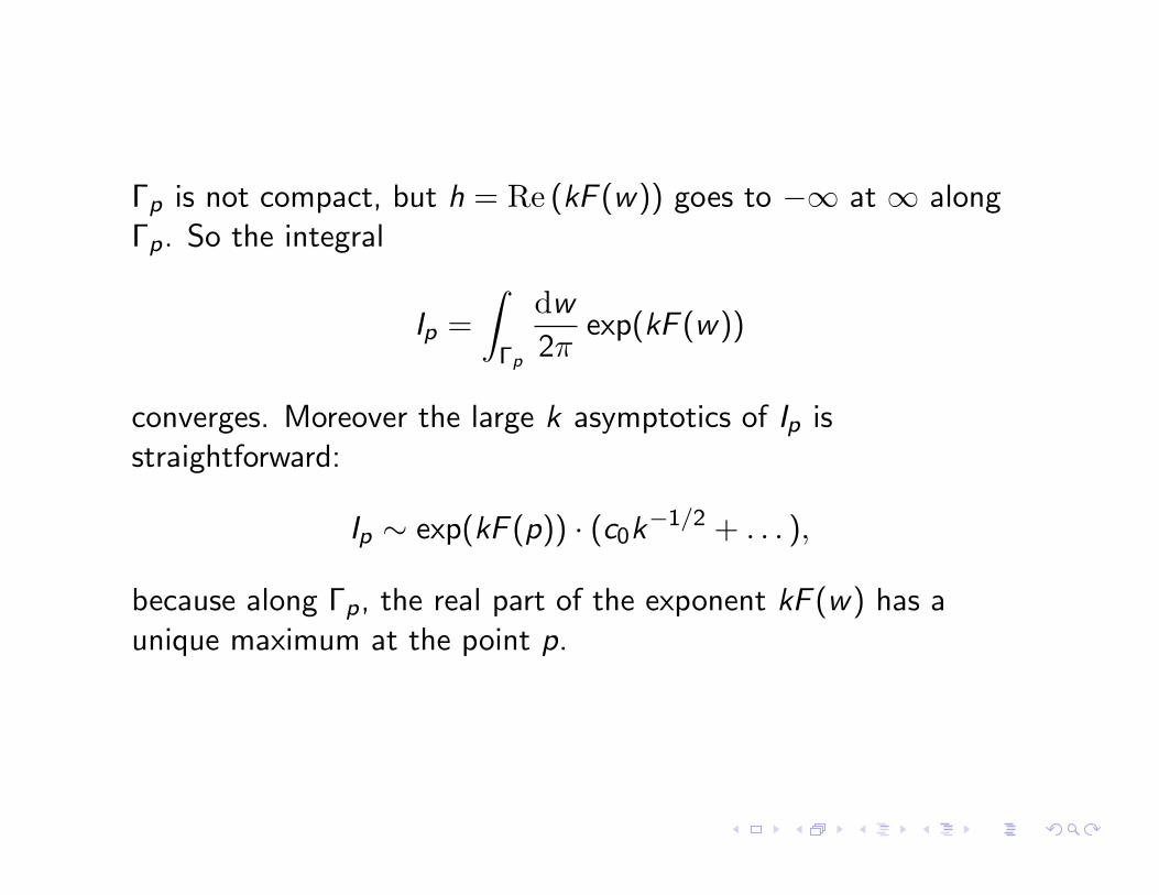
�p is not compact, but h = Re (kF (w)) goes to �1 at 1 along�p.
So the integral
Ip =
Z
�p
dw
2⇡exp(kF (w))
converges. Moreover the large k asymptotics of Ip isstraightforward:
Ip ⇠ exp(kF (p)) · (c0k�1/2 + . . . ),
because along �p, the real part of the exponent kF (w) has aunique maximum at the point p.

�p is not compact, but h = Re (kF (w)) goes to �1 at 1 along�p. So the integral
Ip =
Z
�p
dw
2⇡exp(kF (w))
converges.
Moreover the large k asymptotics of Ip isstraightforward:
Ip ⇠ exp(kF (p)) · (c0k�1/2 + . . . ),
because along �p, the real part of the exponent kF (w) has aunique maximum at the point p.
�p is not compact, but h = Re (kF (w)) goes to �1 at 1 along�p. So the integral
Ip =
Z
�p
dw
2⇡exp(kF (w))
converges. Moreover the large k asymptotics of Ip isstraightforward:
Ip ⇠ exp(kF (p)) · (c0k�1/2 + . . . ),
because along �p, the real part of the exponent kF (w) has aunique maximum at the point p.

Any other cycle � along which the integral converges can beexpanded in terms of the Lefschetz thimbles:
� =X
p
ap�p, ap 2 Z.
After computing the integers ap, it is straightforward to determinethe large k asymptotics of the integral over �, since theasymptotics of the integrals over �p are known. Applying thisprocedure to our integral
Z
�
dw
2⇡ie
kF (w),
we learn what I said before: this integral has a qualitative behaviorsimilar to that of the colored Jones polynomial. The limit n ! 1,k = k0 + n has very di↵erent behavior depending on whether k0 isan integer. (If k0 is not an integer, the large k asymptotics isdominated by two Lefschetz thimbles whose contributions cancel ifk0 is an integer.)

Any other cycle � along which the integral converges can beexpanded in terms of the Lefschetz thimbles:
� =X
p
ap�p, ap 2 Z.
After computing the integers ap, it is straightforward to determinethe large k asymptotics of the integral over �, since theasymptotics of the integrals over �p are known.
Applying thisprocedure to our integral
Z
�
dw
2⇡ie
kF (w),
we learn what I said before: this integral has a qualitative behaviorsimilar to that of the colored Jones polynomial. The limit n ! 1,k = k0 + n has very di↵erent behavior depending on whether k0 isan integer. (If k0 is not an integer, the large k asymptotics isdominated by two Lefschetz thimbles whose contributions cancel ifk0 is an integer.)

Any other cycle � along which the integral converges can beexpanded in terms of the Lefschetz thimbles:
� =X
p
ap�p, ap 2 Z.
After computing the integers ap, it is straightforward to determinethe large k asymptotics of the integral over �, since theasymptotics of the integrals over �p are known. Applying thisprocedure to our integral
Z
�
dw
2⇡ie
kF (w),
we learn what I said before: this integral has a qualitative behaviorsimilar to that of the colored Jones polynomial.
The limit n ! 1,k = k0 + n has very di↵erent behavior depending on whether k0 isan integer. (If k0 is not an integer, the large k asymptotics isdominated by two Lefschetz thimbles whose contributions cancel ifk0 is an integer.)

Any other cycle � along which the integral converges can beexpanded in terms of the Lefschetz thimbles:
� =X
p
ap�p, ap 2 Z.
After computing the integers ap, it is straightforward to determinethe large k asymptotics of the integral over �, since theasymptotics of the integrals over �p are known. Applying thisprocedure to our integral
Z
�
dw
2⇡ie
kF (w),
we learn what I said before: this integral has a qualitative behaviorsimilar to that of the colored Jones polynomial. The limit n ! 1,k = k0 + n has very di↵erent behavior depending on whether k0 isan integer.
(If k0 is not an integer, the large k asymptotics isdominated by two Lefschetz thimbles whose contributions cancel ifk0 is an integer.)

Any other cycle � along which the integral converges can beexpanded in terms of the Lefschetz thimbles:
� =X
p
ap�p, ap 2 Z.
After computing the integers ap, it is straightforward to determinethe large k asymptotics of the integral over �, since theasymptotics of the integrals over �p are known. Applying thisprocedure to our integral
Z
�
dw
2⇡ie
kF (w),
we learn what I said before: this integral has a qualitative behaviorsimilar to that of the colored Jones polynomial. The limit n ! 1,k = k0 + n has very di↵erent behavior depending on whether k0 isan integer. (If k0 is not an integer, the large k asymptotics isdominated by two Lefschetz thimbles whose contributions cancel ifk0 is an integer.)

At this stage, I hope it is fairly clear what we should do tounderstand the analytic continuation to non-integer k of thequantum invariants of knots in R3, and also to understand theasymptotic behavior of the colored Jones polynomial that isstudied in the volume conjecture.
We should define Letschetzthimbles in the space U of complex-valued connections, and in thegauge theory definition of the Jones polynomial, we should replacethe integral over the space U of real connections with a sum ofintegrals over Lefschetz thimbles.
However, it probably is not clear that this will actually lead to auseful new understanding of the Jones polynomial. That wascertainly not clear to me at this stage.

At this stage, I hope it is fairly clear what we should do tounderstand the analytic continuation to non-integer k of thequantum invariants of knots in R3, and also to understand theasymptotic behavior of the colored Jones polynomial that isstudied in the volume conjecture. We should define Letschetzthimbles in the space U of complex-valued connections, and in thegauge theory definition of the Jones polynomial, we should replacethe integral over the space U of real connections with a sum ofintegrals over Lefschetz thimbles.
However, it probably is not clear that this will actually lead to auseful new understanding of the Jones polynomial.
That wascertainly not clear to me at this stage.

At this stage, I hope it is fairly clear what we should do tounderstand the analytic continuation to non-integer k of thequantum invariants of knots in R3, and also to understand theasymptotic behavior of the colored Jones polynomial that isstudied in the volume conjecture. We should define Letschetzthimbles in the space U of complex-valued connections, and in thegauge theory definition of the Jones polynomial, we should replacethe integral over the space U of real connections with a sum ofintegrals over Lefschetz thimbles.
However, it probably is not clear that this will actually lead to auseful new understanding of the Jones polynomial. That wascertainly not clear to me at this stage.

To define the Lefschetz thimbles we want, we need to consider agradient flow equation on the infinite-dimensional space U ofcomplex-valued connections, with Re(ikCS(A)) as a Morsefunction.
Actually, I want to first practice with the case of gradientflow on the infinite-dimensional space U of real connections (on aG -bundle E ! M, M being a three-manifold), with the Morsefunction CS(A). This case is actually familiar to researchers onDonaldson and Floer theories and hence will be familiar to some ofyou. A Riemannian metric on M induces a Riemannian metric onU by
|�A|2 = �Z
MTr �A ^ ?�A
where ? = ?3 is the Hodge star operator on the three-manifold M.We will use this metric on U to define a gradient flow equation.

To define the Lefschetz thimbles we want, we need to consider agradient flow equation on the infinite-dimensional space U ofcomplex-valued connections, with Re(ikCS(A)) as a Morsefunction. Actually, I want to first practice with the case of gradientflow on the infinite-dimensional space U of real connections (on aG -bundle E ! M, M being a three-manifold), with the Morsefunction CS(A).
This case is actually familiar to researchers onDonaldson and Floer theories and hence will be familiar to some ofyou. A Riemannian metric on M induces a Riemannian metric onU by
|�A|2 = �Z
MTr �A ^ ?�A
where ? = ?3 is the Hodge star operator on the three-manifold M.We will use this metric on U to define a gradient flow equation.

To define the Lefschetz thimbles we want, we need to consider agradient flow equation on the infinite-dimensional space U ofcomplex-valued connections, with Re(ikCS(A)) as a Morsefunction. Actually, I want to first practice with the case of gradientflow on the infinite-dimensional space U of real connections (on aG -bundle E ! M, M being a three-manifold), with the Morsefunction CS(A). This case is actually familiar to researchers onDonaldson and Floer theories and hence will be familiar to some ofyou.
A Riemannian metric on M induces a Riemannian metric onU by
|�A|2 = �Z
MTr �A ^ ?�A
where ? = ?3 is the Hodge star operator on the three-manifold M.We will use this metric on U to define a gradient flow equation.

To define the Lefschetz thimbles we want, we need to consider agradient flow equation on the infinite-dimensional space U ofcomplex-valued connections, with Re(ikCS(A)) as a Morsefunction. Actually, I want to first practice with the case of gradientflow on the infinite-dimensional space U of real connections (on aG -bundle E ! M, M being a three-manifold), with the Morsefunction CS(A). This case is actually familiar to researchers onDonaldson and Floer theories and hence will be familiar to some ofyou. A Riemannian metric on M induces a Riemannian metric onU by
|�A|2 = �Z
MTr �A ^ ?�A
where ? = ?3 is the Hodge star operator on the three-manifold M.
We will use this metric on U to define a gradient flow equation.

To define the Lefschetz thimbles we want, we need to consider agradient flow equation on the infinite-dimensional space U ofcomplex-valued connections, with Re(ikCS(A)) as a Morsefunction. Actually, I want to first practice with the case of gradientflow on the infinite-dimensional space U of real connections (on aG -bundle E ! M, M being a three-manifold), with the Morsefunction CS(A). This case is actually familiar to researchers onDonaldson and Floer theories and hence will be familiar to some ofyou. A Riemannian metric on M induces a Riemannian metric onU by
|�A|2 = �Z
MTr �A ^ ?�A
where ? = ?3 is the Hodge star operator on the three-manifold M.We will use this metric on U to define a gradient flow equation.

The flow equation will be a di↵erential equation on thefour-manifold X = M ⇥ R, where R is parametrized by the “time”;one can think of the flow equation as evolving a three-dimensionalconnection in “time.”
Concretely, the flow equation is
@A
@t= ��CS(A)
�A= � ?3 F ,
where F = dA+ A ^ A is the curvature. Now a couple of miracleshappen: This equation a priori has no reason to be elliptic or tohave four-dimensional symmetry. But it turns out that theequation is actually a gauge-fixed version of the instanton equationF
+ = 0, which is elliptic modulo the gauge group and has fullfour-dimensional symmetry (that is, it is naturally defined on anyoriented four-manifold X , not necessarily M ⇥ R for some M).These miracles are very well known to resarchers on Donaldson andFloer theory, where they play an important role.
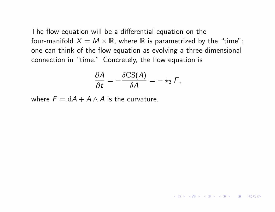
The flow equation will be a di↵erential equation on thefour-manifold X = M ⇥ R, where R is parametrized by the “time”;one can think of the flow equation as evolving a three-dimensionalconnection in “time.” Concretely, the flow equation is
@A
@t= ��CS(A)
�A= � ?3 F ,
where F = dA+ A ^ A is the curvature.
Now a couple of miracleshappen: This equation a priori has no reason to be elliptic or tohave four-dimensional symmetry. But it turns out that theequation is actually a gauge-fixed version of the instanton equationF
+ = 0, which is elliptic modulo the gauge group and has fullfour-dimensional symmetry (that is, it is naturally defined on anyoriented four-manifold X , not necessarily M ⇥ R for some M).These miracles are very well known to resarchers on Donaldson andFloer theory, where they play an important role.

The flow equation will be a di↵erential equation on thefour-manifold X = M ⇥ R, where R is parametrized by the “time”;one can think of the flow equation as evolving a three-dimensionalconnection in “time.” Concretely, the flow equation is
@A
@t= ��CS(A)
�A= � ?3 F ,
where F = dA+ A ^ A is the curvature. Now a couple of miracleshappen: This equation a priori has no reason to be elliptic or tohave four-dimensional symmetry.
But it turns out that theequation is actually a gauge-fixed version of the instanton equationF
+ = 0, which is elliptic modulo the gauge group and has fullfour-dimensional symmetry (that is, it is naturally defined on anyoriented four-manifold X , not necessarily M ⇥ R for some M).These miracles are very well known to resarchers on Donaldson andFloer theory, where they play an important role.

The flow equation will be a di↵erential equation on thefour-manifold X = M ⇥ R, where R is parametrized by the “time”;one can think of the flow equation as evolving a three-dimensionalconnection in “time.” Concretely, the flow equation is
@A
@t= ��CS(A)
�A= � ?3 F ,
where F = dA+ A ^ A is the curvature. Now a couple of miracleshappen: This equation a priori has no reason to be elliptic or tohave four-dimensional symmetry. But it turns out that theequation is actually a gauge-fixed version of the instanton equationF
+ = 0, which is elliptic modulo the gauge group and has fullfour-dimensional symmetry (that is, it is naturally defined on anyoriented four-manifold X , not necessarily M ⇥ R for some M).
These miracles are very well known to resarchers on Donaldson andFloer theory, where they play an important role.
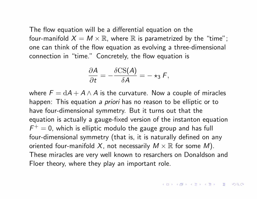
The flow equation will be a di↵erential equation on thefour-manifold X = M ⇥ R, where R is parametrized by the “time”;one can think of the flow equation as evolving a three-dimensionalconnection in “time.” Concretely, the flow equation is
@A
@t= ��CS(A)
�A= � ?3 F ,
where F = dA+ A ^ A is the curvature. Now a couple of miracleshappen: This equation a priori has no reason to be elliptic or tohave four-dimensional symmetry. But it turns out that theequation is actually a gauge-fixed version of the instanton equationF
+ = 0, which is elliptic modulo the gauge group and has fullfour-dimensional symmetry (that is, it is naturally defined on anyoriented four-manifold X , not necessarily M ⇥ R for some M).These miracles are very well known to resarchers on Donaldson andFloer theory, where they play an important role.

It turns out that the same miracles happen when we do gradientflow on U , with the Morse function Re(ikCS(A)) and the obviousKahler metric on U
|�A|2 = �Z
MTr �A ^ ?�A.
The gradient flow equation is a gauge-fixed version of an ellipticdi↵erential equation that has full four-dimensional symmetry. Thisequation can be seen as a four-dimensional cousin of N. Hitchin’scelebrated two-dimension equation. It is an equation for a pairA,�, where A is a connection on a G -bundle E ! X , X being anoriented four-manifold, and � 2 ⌦1(X , ad(E )) is a one-form on X
valued in ad(E ). The equations (for simplicity I take k real) read
F � � ^ �+ ?dA� = 0, dA ? � = 0.
They are flow equations for the three-dimensional connectionA = A+ i�.

It turns out that the same miracles happen when we do gradientflow on U , with the Morse function Re(ikCS(A)) and the obviousKahler metric on U
|�A|2 = �Z
MTr �A ^ ?�A.
The gradient flow equation is a gauge-fixed version of an ellipticdi↵erential equation that has full four-dimensional symmetry.
Thisequation can be seen as a four-dimensional cousin of N. Hitchin’scelebrated two-dimension equation. It is an equation for a pairA,�, where A is a connection on a G -bundle E ! X , X being anoriented four-manifold, and � 2 ⌦1(X , ad(E )) is a one-form on X
valued in ad(E ). The equations (for simplicity I take k real) read
F � � ^ �+ ?dA� = 0, dA ? � = 0.
They are flow equations for the three-dimensional connectionA = A+ i�.

It turns out that the same miracles happen when we do gradientflow on U , with the Morse function Re(ikCS(A)) and the obviousKahler metric on U
|�A|2 = �Z
MTr �A ^ ?�A.
The gradient flow equation is a gauge-fixed version of an ellipticdi↵erential equation that has full four-dimensional symmetry. Thisequation can be seen as a four-dimensional cousin of N. Hitchin’scelebrated two-dimension equation.
It is an equation for a pairA,�, where A is a connection on a G -bundle E ! X , X being anoriented four-manifold, and � 2 ⌦1(X , ad(E )) is a one-form on X
valued in ad(E ). The equations (for simplicity I take k real) read
F � � ^ �+ ?dA� = 0, dA ? � = 0.
They are flow equations for the three-dimensional connectionA = A+ i�.

It turns out that the same miracles happen when we do gradientflow on U , with the Morse function Re(ikCS(A)) and the obviousKahler metric on U
|�A|2 = �Z
MTr �A ^ ?�A.
The gradient flow equation is a gauge-fixed version of an ellipticdi↵erential equation that has full four-dimensional symmetry. Thisequation can be seen as a four-dimensional cousin of N. Hitchin’scelebrated two-dimension equation. It is an equation for a pairA,�, where A is a connection on a G -bundle E ! X , X being anoriented four-manifold, and � 2 ⌦1(X , ad(E )) is a one-form on X
valued in ad(E ).
The equations (for simplicity I take k real) read
F � � ^ �+ ?dA� = 0, dA ? � = 0.
They are flow equations for the three-dimensional connectionA = A+ i�.

It turns out that the same miracles happen when we do gradientflow on U , with the Morse function Re(ikCS(A)) and the obviousKahler metric on U
|�A|2 = �Z
MTr �A ^ ?�A.
The gradient flow equation is a gauge-fixed version of an ellipticdi↵erential equation that has full four-dimensional symmetry. Thisequation can be seen as a four-dimensional cousin of N. Hitchin’scelebrated two-dimension equation. It is an equation for a pairA,�, where A is a connection on a G -bundle E ! X , X being anoriented four-manifold, and � 2 ⌦1(X , ad(E )) is a one-form on X
valued in ad(E ). The equations (for simplicity I take k real) read
F � � ^ �+ ?dA� = 0, dA ? � = 0.
They are flow equations for the three-dimensional connectionA = A+ i�.

It turns out that the same miracles happen when we do gradientflow on U , with the Morse function Re(ikCS(A)) and the obviousKahler metric on U
|�A|2 = �Z
MTr �A ^ ?�A.
The gradient flow equation is a gauge-fixed version of an ellipticdi↵erential equation that has full four-dimensional symmetry. Thisequation can be seen as a four-dimensional cousin of N. Hitchin’scelebrated two-dimension equation. It is an equation for a pairA,�, where A is a connection on a G -bundle E ! X , X being anoriented four-manifold, and � 2 ⌦1(X , ad(E )) is a one-form on X
valued in ad(E ). The equations (for simplicity I take k real) read
F � � ^ �+ ?dA� = 0, dA ? � = 0.
They are flow equations for the three-dimensional connectionA = A+ i�.

Something unexpected happens, though it took a while for theimplications to sink in.
I actually had studied these equationsbefore, in my work with A. Kapustin on gauge theory andgeometric Langlands. In a moment we will discuss why thisconnection is relevant. (These equations – sometimes called theKW equations – have been studied recently in a series of papers byC. Taubes and also by M. Gagliardo and K. Uhlenbeck.)

Something unexpected happens, though it took a while for theimplications to sink in. I actually had studied these equationsbefore, in my work with A. Kapustin on gauge theory andgeometric Langlands. In a moment we will discuss why thisconnection is relevant.
(These equations – sometimes called theKW equations – have been studied recently in a series of papers byC. Taubes and also by M. Gagliardo and K. Uhlenbeck.)

Something unexpected happens, though it took a while for theimplications to sink in. I actually had studied these equationsbefore, in my work with A. Kapustin on gauge theory andgeometric Langlands. In a moment we will discuss why thisconnection is relevant. (These equations – sometimes called theKW equations – have been studied recently in a series of papers byC. Taubes and also by M. Gagliardo and K. Uhlenbeck.)
Now we can define a Lefschetz thimble for any choice of a complexflat connection A⇢ on M, associated to ⇢ : ⇡1(M) ! GC.
We workon the four-manifold X = M ⇥ R+
and define the thimble �⇢ to consist of all complex connectionsA = A+ i� on M ⇥ {0} ⇢ M ⇥ R+ that are boundary values ofsolutions of the KW equations on M ⇥ R+ that approach A⇢ atinfinity.

Now we can define a Lefschetz thimble for any choice of a complexflat connection A⇢ on M, associated to ⇢ : ⇡1(M) ! GC. We workon the four-manifold X = M ⇥ R+
and define the thimble �⇢ to consist of all complex connectionsA = A+ i� on M ⇥ {0} ⇢ M ⇥ R+ that are boundary values ofsolutions of the KW equations on M ⇥ R+ that approach A⇢ atinfinity.

For a general M, there are various choices of ⇢. To understand theusual quantum knot invariants in this way, we would need toexpress the integration cycle U ⇢ U as a linear combination of thethimbles �⇢. This is technically tricky and also the sort of answer itleads to is not so simple as there will be “Stokes phenomena.” (Ithink it is likely that some things studied in the literature can beunderstood in this way and I did some very special cases in mypaper on “Analytic Continuation Of Chern-Simons Theory.”)
However, now we can see what is special about knots in R3 (or S3,but in a moment R3 will be better). Since the fundamental groupof R3 is trivial, any flat connection on R3 is gauge-equivalent tothe trivial one A = 0. There is only one Lefschetz thimble �0, andhence instead of integration over U to define the Jones polynomial,we can define the Jones polynomial by integration over �0.

For a general M, there are various choices of ⇢. To understand theusual quantum knot invariants in this way, we would need toexpress the integration cycle U ⇢ U as a linear combination of thethimbles �⇢. This is technically tricky and also the sort of answer itleads to is not so simple as there will be “Stokes phenomena.” (Ithink it is likely that some things studied in the literature can beunderstood in this way and I did some very special cases in mypaper on “Analytic Continuation Of Chern-Simons Theory.”)
However, now we can see what is special about knots in R3 (or S3,but in a moment R3 will be better). Since the fundamental groupof R3 is trivial, any flat connection on R3 is gauge-equivalent tothe trivial one A = 0.
There is only one Lefschetz thimble �0, andhence instead of integration over U to define the Jones polynomial,we can define the Jones polynomial by integration over �0.

For a general M, there are various choices of ⇢. To understand theusual quantum knot invariants in this way, we would need toexpress the integration cycle U ⇢ U as a linear combination of thethimbles �⇢. This is technically tricky and also the sort of answer itleads to is not so simple as there will be “Stokes phenomena.” (Ithink it is likely that some things studied in the literature can beunderstood in this way and I did some very special cases in mypaper on “Analytic Continuation Of Chern-Simons Theory.”)
However, now we can see what is special about knots in R3 (or S3,but in a moment R3 will be better). Since the fundamental groupof R3 is trivial, any flat connection on R3 is gauge-equivalent tothe trivial one A = 0. There is only one Lefschetz thimble �0, andhence instead of integration over U to define the Jones polynomial,we can define the Jones polynomial by integration over �0.

So the Jones polynomial isZ
�0
DA exp(ikCS(A)) · TrR Hol(A,K )
where �0 is the space of solutions of the KW equations onR3 ⇥ R+ that vanish on M ⇥ {1} and A is the restriction ofA+ i� to M ⇥ {0}:

My work with Kapustin involved a twisted version of N = 4 superYang-Mills theory in four dimensions.
The twisted theory“localizes” on the space of solutions of the KW equations. Thisspace (if we require our connections to vanish on R3 ⇥ {1}) is theLefschetz thimble that we have to integrate over to get the Jonespolynomial. The upshot is that the Jones polynomial for a knot inR3 can be computed from a path integral of N = 4 superYang-Mills theory on X = R3 ⇥ R+, with a slightly unusualboundary condition on R3 ⇥ {0}.

My work with Kapustin involved a twisted version of N = 4 superYang-Mills theory in four dimensions. The twisted theory“localizes” on the space of solutions of the KW equations.
Thisspace (if we require our connections to vanish on R3 ⇥ {1}) is theLefschetz thimble that we have to integrate over to get the Jonespolynomial. The upshot is that the Jones polynomial for a knot inR3 can be computed from a path integral of N = 4 superYang-Mills theory on X = R3 ⇥ R+, with a slightly unusualboundary condition on R3 ⇥ {0}.

My work with Kapustin involved a twisted version of N = 4 superYang-Mills theory in four dimensions. The twisted theory“localizes” on the space of solutions of the KW equations. Thisspace (if we require our connections to vanish on R3 ⇥ {1}) is theLefschetz thimble that we have to integrate over to get the Jonespolynomial.
The upshot is that the Jones polynomial for a knot inR3 can be computed from a path integral of N = 4 superYang-Mills theory on X = R3 ⇥ R+, with a slightly unusualboundary condition on R3 ⇥ {0}.

My work with Kapustin involved a twisted version of N = 4 superYang-Mills theory in four dimensions. The twisted theory“localizes” on the space of solutions of the KW equations. Thisspace (if we require our connections to vanish on R3 ⇥ {1}) is theLefschetz thimble that we have to integrate over to get the Jonespolynomial. The upshot is that the Jones polynomial for a knot inR3 can be computed from a path integral of N = 4 superYang-Mills theory on X = R3 ⇥ R+, with a slightly unusualboundary condition on R3 ⇥ {0}.

Unfortunately, until quantum field theory is more familiar, this isgoing to be a hard answer for mathematicians to understand – justlike the formula for the Jones polynomial by integration over thespace U of real connections – because infinite-dimensionalintegration is unfamiliar.
(But the conclusion we just reachedcould be verified mathematically, in an asymptotic expansion neark = 1 or q = 1. Here one would run into an expansion inFeynman diagrams as in the work of Kontsevich and others onknot invariants related to the gauge theory.)

Unfortunately, until quantum field theory is more familiar, this isgoing to be a hard answer for mathematicians to understand – justlike the formula for the Jones polynomial by integration over thespace U of real connections – because infinite-dimensionalintegration is unfamiliar. (But the conclusion we just reachedcould be verified mathematically, in an asymptotic expansion neark = 1 or q = 1. Here one would run into an expansion inFeynman diagrams as in the work of Kontsevich and others onknot invariants related to the gauge theory.)

However, one more step brings us into a world that is accessiblemathematically, and also gives a new explanation of why the Jonespolynomial is a Laurent polynomial in q.
The step in question wasalso a key step in my work with Kapustin, and, more generally, inmuch of the work of physicists on the supersymmetric gaugetheory in question. This is electric-magnetic duality, thefour-dimensional analog of mirror symmetry in two dimensions.N = 4 super Yang-Mills theory with gauge group G and “couplingparameter” ⌧ is equivalent to the same theory with gauge groupG
_ – the Langlands or GNO dual of G – and coupling parameter⌧_ = �1/ng⌧ (ng is as before the ratio of length squared of longand short roots).
However, one more step brings us into a world that is accessiblemathematically, and also gives a new explanation of why the Jonespolynomial is a Laurent polynomial in q. The step in question wasalso a key step in my work with Kapustin, and, more generally, inmuch of the work of physicists on the supersymmetric gaugetheory in question.
This is electric-magnetic duality, thefour-dimensional analog of mirror symmetry in two dimensions.N = 4 super Yang-Mills theory with gauge group G and “couplingparameter” ⌧ is equivalent to the same theory with gauge groupG
_ – the Langlands or GNO dual of G – and coupling parameter⌧_ = �1/ng⌧ (ng is as before the ratio of length squared of longand short roots).

However, one more step brings us into a world that is accessiblemathematically, and also gives a new explanation of why the Jonespolynomial is a Laurent polynomial in q. The step in question wasalso a key step in my work with Kapustin, and, more generally, inmuch of the work of physicists on the supersymmetric gaugetheory in question. This is electric-magnetic duality, thefour-dimensional analog of mirror symmetry in two dimensions.N = 4 super Yang-Mills theory with gauge group G and “couplingparameter” ⌧ is equivalent to the same theory with gauge groupG
_ – the Langlands or GNO dual of G – and coupling parameter⌧_ = �1/ng⌧ (ng is as before the ratio of length squared of longand short roots).

To learn anything about our problem, we need to know whathappens to the boundary condition at R3 ⇥ {0} underelectric-magnetic duality. (This question is the analog of asking –in mirror symmetry – what is the object in the Fukaya categorythat is mirror to a given coherent sheaf.)
For the boundarycondition that appeared in the derivation we have just given, thedual boundary condition was described by D. Gaiotto and me anumber of years ago. It is a somewhat unusual elliptic boundarycondition that is related to the work of W. Nahm on monopoles; Iwill describe it at the workshop tomorrow.For now, just let me saythat this boundary condition is similar to a standard local ellipticboundary condition and has the e↵ect of reducing tofinite-dimensional spaces of solutions of the KW equations.

To learn anything about our problem, we need to know whathappens to the boundary condition at R3 ⇥ {0} underelectric-magnetic duality. (This question is the analog of asking –in mirror symmetry – what is the object in the Fukaya categorythat is mirror to a given coherent sheaf.) For the boundarycondition that appeared in the derivation we have just given, thedual boundary condition was described by D. Gaiotto and me anumber of years ago.
It is a somewhat unusual elliptic boundarycondition that is related to the work of W. Nahm on monopoles; Iwill describe it at the workshop tomorrow.For now, just let me saythat this boundary condition is similar to a standard local ellipticboundary condition and has the e↵ect of reducing tofinite-dimensional spaces of solutions of the KW equations.

To learn anything about our problem, we need to know whathappens to the boundary condition at R3 ⇥ {0} underelectric-magnetic duality. (This question is the analog of asking –in mirror symmetry – what is the object in the Fukaya categorythat is mirror to a given coherent sheaf.) For the boundarycondition that appeared in the derivation we have just given, thedual boundary condition was described by D. Gaiotto and me anumber of years ago. It is a somewhat unusual elliptic boundarycondition that is related to the work of W. Nahm on monopoles; Iwill describe it at the workshop tomorrow.
For now, just let me saythat this boundary condition is similar to a standard local ellipticboundary condition and has the e↵ect of reducing tofinite-dimensional spaces of solutions of the KW equations.

To learn anything about our problem, we need to know whathappens to the boundary condition at R3 ⇥ {0} underelectric-magnetic duality. (This question is the analog of asking –in mirror symmetry – what is the object in the Fukaya categorythat is mirror to a given coherent sheaf.) For the boundarycondition that appeared in the derivation we have just given, thedual boundary condition was described by D. Gaiotto and me anumber of years ago. It is a somewhat unusual elliptic boundarycondition that is related to the work of W. Nahm on monopoles; Iwill describe it at the workshop tomorrow.For now, just let me saythat this boundary condition is similar to a standard local ellipticboundary condition and has the e↵ect of reducing tofinite-dimensional spaces of solutions of the KW equations.

In this situation
after making the duality transformation,
the moduli space ofsolutions has expected dimension 0 and we just have to “count”(with signs, as in Donaldson theory) the number bn of solutions fora given value n of the second Chern class. The boundary conditionsdepend on the knot K and the choice of the representation R bywhich it is labeled (some details at the workshop tomorrow).

In this situation
after making the duality transformation, the moduli space ofsolutions has expected dimension 0 and we just have to “count”(with signs, as in Donaldson theory) the number bn of solutions fora given value n of the second Chern class.
The boundary conditionsdepend on the knot K and the choice of the representation R bywhich it is labeled (some details at the workshop tomorrow).

In this situation
after making the duality transformation, the moduli space ofsolutions has expected dimension 0 and we just have to “count”(with signs, as in Donaldson theory) the number bn of solutions fora given value n of the second Chern class. The boundary conditionsdepend on the knot K and the choice of the representation R bywhich it is labeled (some details at the workshop tomorrow).

The path integral gives
Zq(K ;R) =X
n
bnqn
where q = exp(2⇡i/ngk) and bn is the “number” of solutions forgiven second Chern class n. This exhibits the Jones polynomialand the related quantum invariants of knots in three dimensions as“Laurent polynomials” in q with integer coe�cients.
I put“Laurent polynomials” in quotes because the powers of q areshifted from integers in a way that depends only on therepresentations, so for instance the Jones polynomial of a knotwith this normalization is q1/2 times a Laurent series in q.

The path integral gives
Zq(K ;R) =X
n
bnqn
where q = exp(2⇡i/ngk) and bn is the “number” of solutions forgiven second Chern class n. This exhibits the Jones polynomialand the related quantum invariants of knots in three dimensions as“Laurent polynomials” in q with integer coe�cients. I put“Laurent polynomials” in quotes because the powers of q areshifted from integers in a way that depends only on therepresentations, so for instance the Jones polynomial of a knotwith this normalization is q1/2 times a Laurent series in q.