BLUP for phenotypic selection in plant breedingand variety testing

H. P. Piepho Æ J. Mohring Æ A. E. Melchinger ÆA. Buchse

Received: 12 October 2006 / Accepted: 25 April 2007 / Published online: 19 July 2007

� Springer Science+Business Media B.V. 2007

Abstract Best linear unbiased prediction (BLUP) is

a standard method for estimating random effects of a

mixed model. This method was originally developed in

animal breeding for estimation of breeding values and

is now widely used in many areas of research. It does

not, however, seem to have gained the same popularity

in plant breeding and variety testing as it has in animal

breeding. In plants, application of mixed models with

random genetic effects has up until recently been

mainly restricted to the estimation of genetic and non-

genetic components of variance, whereas estimation of

genotypic values is mostly based on a model with fixed

effects. This paper reviews recent developments in the

application of BLUP in plant breeding and variety

testing. These include the use of pedigree information

to model and exploit genetic correlation among

relatives and the use of flexible variance–covariance

structures for genotype-by-environment interaction.

We demonstrate that BLUP has good predictive

accuracy compared to other procedures. While pedi-

gree information is often included via the so-called

numerator relationship matrix ðAÞ, we stress that it is

frequently straightforward to exploit the same infor-

mation by a simple mixed model without explicit

reference to the A-matrix.

Keywords Mixed model � Breeding value �Pedigree � Genetic effect � Genotypic value

Introduction

Both the development of new cultivars as well as

the recommendation of newly released varieties

require a selection to be made among a larger set of

candidate genotypes, so estimation of genotypic

values is at the heart of any breeding effort.

Analysis of metric data from plant breeding and

variety trials can usually be based on a mixed linear

model of the form

y ¼ XbþZuþ e; ð1Þ

where y is the vector of observations, b and u are

vectors of fixed and random effects, respectively, X

and Z are the associated design matrices, and e is a

random residual vector. The random effects are

assumed to be distributed as u � MVN 0;Gð Þ and

e � MVN 0;Rð Þ, where MVN l;Vð Þ denotes the

multivariate normal distribution with mean vector l

and variance–covariance matrix V. The fixed effects

can be estimated by Best Linear Unbiased Estimation

This paper is dedicated to Prof. Dr. Wolfgang Kohler

(University of Giessen, Germany) on the occasion of his 65th

birthday.

H. P. Piepho (&) � J. Mohring � A. E. Melchinger �A. Buchse

Bioinformatics Unit, University of Hohenheim,

Fruwirthstrasse 23, 70599 Stuttgart, Germany

e-mail: piepho@uni-hohenheim.de

123

Euphytica (2008) 161:209–228

DOI 10.1007/s10681-007-9449-8

(BLUE), while random effects are estimated by Best

Linear Unbiased Prediction (BLUP). In practice,

BLUE and BLUP need to be replaced by ‘‘empirical’’

BLUE and BLUP, respectively, meaning that vari-

ance components in G and R need to be replaced by

their estimates, obtained preferably by Restricted

Maximum Likelihood (REML) (Patterson and

Thompson 1971). Both BLUE and BLUP may be

computed by solving the Mixed Model Equations

(MME), given by (Henderson 1986; Searle et al.

1992)

X0R�1X X0R�1ZZ0R�1X Z0R�1Zþ G�1

� �b

u

� �¼ X0R�1y

Z0R�1y

� �:

ð2Þ

Often in variety testing and the development of new

varieties, genotype effects are considered as fixed and

thus become part of b in the mixed model. When

genotypes can be regarded as random, however,

genotypic effects become part of u and thus are

estimated by BLUP. The present paper is concerned

with applications where u contains the genotypic or

genetic effects of interest.

By genetic effects, we refer to a decomposition of

the genotypic value into component effects with a

genetic interpretation. One such decomposition is

into additive and non-additive effects (dominance,

epistasis). Alternatively, in a diallel or factorial, the

genotypic value of a hybrid may be partitioned into

genetic effects for general and specific combining

ability. The ultimate objective in breeding applica-

tions usually is prediction of the genotypic value of a

candidate genotype. Thus, our discussion here is

mainly in terms of genotypic values.

One major property of BLUP is shrinkage towards

the mean, which anticipates regression of progeny to

the mean observed by every breeder (Hill and

Rosenberger 1985). Shrinkage is often a desirable

statistical property of an estimator, as it increases

accuracy, when the bias incurred from shrinkage is

more than offset by the reduction in variance, thus

leading to a smaller mean squared error (MSE). This

is true not only for BLUP, but also for other

shrinkage estimators in common usage (Copas

1983; Robinson 1991; Miller 2002). Finally, under

certain fairly general assumptions, BLUP maximizes

the correlation of true genotypic values and predicted

genotypic values (Searle et al. 1992), which is the

primary aim of breeders.

There is often considerable debate as to whether

it is reasonable to assume that genotypes are a

random factor. An argument sometimes put forward

against this assumption is that genotypes are not

usually a random sample from a defined population

as one would obtain, e.g., in survey sampling,

because genotypes under test are the result of

considerable selection effort. While this is certainly

true in most cases, it is often reasonable to regard

the genotypes under test as a random sample from

some hypothetical population of genotypes that

could have arisen as a result of the selection process

leading to the genotypes currently available (Piepho

and Mohring, 2006). Furthermore, the theory of

James and Stein (1961) justifies the use of BLUP

even if we think of the parameters as fixed, provided

the number of parameters is large (Lee et al. 2006,

pp. 151–152). James and Stein (1961) showed that

BLUE can be beaten by shrinkage estimation, when

the effect in question has more than two levels.

Note, also, that in a Bayesian framework, the

distinction between fixed and random effects van-

ishes. To a Bayesian, all effects are random, because

all parameters of a model have a prior density,

reflecting the uncertainty about parameter values

(Gianola and Fernando 1986). It is also useful to

realize that BLUE can be regarded as a limiting case

of BLUP, when G�1 in the mixed model equations

tends to zero, so that the MME reduce to ordinary

least squares equations. To a Bayesian this simply

means that prior knowledge about u is ignored

(Gianola and Fernando 1986; Sorensen and Gianola

2002). The most critical practical issue is whether

good estimates of G can be obtained (Smith et al.

2005). Whether or not this is the case, depends

foremost on sample size and on the availability of

complete data back to a base population, to which

genetic variance components refer (Thompson 1973,

1979; Van der Werf and de Boer 1990; Piepho and

Mohring 2006). Only when the data does not permit

accurate estimation of genetic variance components

or when the main emphasis of analysis is on the

comparison of genotypes by a statistical test, does it

seem reasonable to take genotypes as fixed.

BLUP does not appear to have gained the same

popularity as in animal breeding, where it is the

standard procedure. There are some applications in

210 Euphytica (2008) 161:209–228

123

forestry and perennial crops (White and Hodge 1989;

Durel et al. 1998; Dutkowski et al. 2002; Xiang and

Li 2003), but publications using BLUP with annual

crops are less abundant. One reason may be that plant

breeding programmes usually yield a relatively large

amount of phenotypic data per genotype from series

of experiments, so BLUE and BLUP often do not

provide grossly different results. This may lead to the

false impression that the choice of estimator is not

important. Also, in animal breeding, BLUP or similar

procedures are usually a necessity due to lack of

direct observations, such as in the case of breeding

values of sires for milk yield in dairy, while this type

of problem occurs less frequently in plant breeding

(one example in kind is general combining ability,

which cannot be directly observed). In addition,

animal breeding programmes typically comprise a

very large number of genotypes, so genetic variance

component estimates are very accurate. By contrast,

genetic variance estimates in plant breeding applica-

tions are often relatively inaccurate due to more

limited numbers of genotypes and more complex

genetic covariance structures.

A desirable feature of BLUP is its ability to

borrow strength from relatives by exploiting genetic

correlation arising from the pedigree. The closer the

genetic correlation with relatives, the more informa-

tion can be extracted from phenotypic information on

relatives. The most common approach to exploiting

pedigree information involves use of the so-called

numerator relationship matrix (Mrode 1996), com-

puted from the coefficient of coancestry. As is

emphasised in this paper, one may also consider

mixed models, which incorporate pedigree informa-

tion in simple pedigrees without explicitly using the

numerator relationship matrix.

The purpose of this paper is to review applications

of BLUP in plant breeding and variety testing and to

underline the potential advantages of BLUP, which

have been demonstrated in a considerable number of

publications. The paper is organized as follows. The

next section deals with applications of BLUP that do

not exploit pedigree information. Sections 3 and 4

consider the use of pedigree information. Section 3

reviews applications that exploit the coefficient of

coancestry, while section 4 deals with pedigree-based

BLUP when the coefficient of coancestry is not

utilized. Some examples are given in Section 5. Much

of the theoretical work on pedigree-based BLUP

using the coefficient of coancestry was done in an

animal breeding context, where this methodology

originated. We give a cursory account of some of the

theoretical underpinnings and statistical assumptions

as relevant in a plant breeding context. The main

focus is on BLUP of genotypic values for selection in

annual crops.

BLUP without pedigree information

The simplest case of BLUP occurs when a single

genotypic effect in a linear model is taken as

independent random variable without any correlation

imposed by the pedigree. Thus, genotypes are con-

sidered as independent, and pedigree information is

not exploited. Gain in accuracy compared to BLUE

therefore stems mainly from the shrinkage property,

while genetic covariance between related genotypes

plays no role. In multi-environment trials, genetic

correlation among performances of the same genotype

in different environments may be exploited.

Single trials

Cullis et al. (1989) and Stroup and Mulitze (1991)

showed that BLUP of genotypic values in single trials

can be enhanced by a spatial model for local field

trends. Cullis et al. (1989) focused on trials, where a

large number of new entries are tested without

replication. A particular class of designs for such

settings are the augmented designs, where some

replicated design for checks is augmented by unre-

plicated entries. Federer (1998) proposed to analyse

such designs (and other incomplete block designs)

assuming random genotypic values. Santos et al.

(2002) showed by simulation that BLUP in aug-

mented designs may be hampered by poor estimates

of genetic variance components. With known vari-

ance components, BLUP was always superior to

BLUE. Cullis et al. (2006) suggested a strategy to

find optimal designs for early-generation variety

testing, when analysis is to be based on a spatial

model and genotype effects are to be estimated by

BLUP. The objective criterion is based on an

approximation to the expected genetic gain from

selection.

Euphytica (2008) 161:209–228 211

123

Multi-environment trials

Hill and Rosenberger (1985) considered BLUP of

genotype main effects in genotype-by-environment

data and found BLUP to outperform BLUE. Yan

et al. (2002) compared on-farm strip trials versus

replicated performance trials with wheat (Triticum

aestivum) based on BLUP of genotype effects. Yan

and Rajcan (2003) used BLUP in soybean (Glycine

max) based on a three-way model (genotype-by-

location-by-year).

Gauch (1988) popularized the Additive Main

Effect Multiplicative Interaction (AMMI) model for

genotype-environment data and pointed out that

retention of a small number of multiplicative terms

leads to shrinkage of estimated interaction effects

compared to ordinary least squares estimates based

on the usual two-way ANOVA model. The AMMI

model suggested by Gauch (1988) is a fixed effects

model. He showed by cross validation that the

resulting estimates of genotype-by-environment

means were more accurate than ordinary least squares

estimates. Essentially, the AMMI model improves

accuracy of genotypic mean estimates for an envi-

ronment by borrowing strength from other environ-

ments via multiplicative interaction terms. The

shrinkage property of AMMI led Piepho (1994) to

conduct a comparison with BLUP based on a two-

way ANOVA model. This study provided evidence

that BLUP was more accurate than the fixed effects

AMMI model. Further improvement is possible by a

mixed-model version of the AMMI model, also

known as the factor-analytic model (Piepho 1997),

as demonstrated in a cross-validation study by Piepho

(1998). The factor-analytic model gleans information

from correlated environments via (factor-analytic)

correlation of genotype-by-environment effects. A

parallel literature has developed various alternative

shrinkage factors for the AMMI model (Cornelius

et al. 1996; Cornelius and Crossa 1999; Moreno-

Gonzalez et al. 2003, 2004), including a Bayesian

approach (Viele and Srinivasan 2000), but these do

not strictly fall in the mixed model framework.

Combination of single trial information based on

spatial models with flexible variance–covariance

structures for genotype-by-environment effects, e.g.

heteroscedastic and factor-analytic, has been sug-

gested, e.g., by Frensham et al. (1997), Cullis et al.

(1998) and Smith et al. (2001b). BLUP of variety

effects based on such models is now routinely used in

the analysis of crop variety evaluation data in

Australia (Smith et al. 2001a, 2005).

Curnow (1988) demonstrated that use of correlated

information on treatment effects is beneficial when

selecting the best treatment. This idea was taken up

by Atlin (2000), who investigated the response to

selection in a subdivided target region. Piepho and

Mohring (2005) put this approach in a BLUP

framework and showed that fitting a genetic correla-

tion structure across sub-regions can improve predic-

tions for target regions by exploiting information

from adjacent sub-regions.

Plant breeding data from multiple environments

are notoriously unbalanced, as poor performers are

discarded every year, while new entries are added to

the system. Piepho and Mohring (2006) have shown

based on the theory of Rubin (1976) and Little and

Rubin (1987, 2002) as well as by simulation that

selection is ignorable so long as all data that have

been used in selection decisions are included in the

analysis. This is in agreement with accounts dealing

with pedigree-based BLUP in animal breeding

(Thompson 1973; Henderson 1975) (see sect. 3),

though most of the publications in that area do not

mention Rubin (1976) or Little and Rubin (1987).

One notable exception is Im et al. (1989).

Pedigree-based BLUP using the coefficient of

coancestry

Exploitation of pedigree information in animal

breeding is mostly based on the numerator relation-

ship matrix, usually denoted as A, which is computed

from the coefficient of coancestry (kinship, consan-

guinity) hxy (Falconer and Mackay 1996, p.153)

between genotypes x and y as A ¼ 2hxy

� �, assuming

relatives are not inbred. Breeding values are consid-

ered as random effects with variance–covariance

matrix Ar2A, where r2

A is the additive genetic variance

component. Non-additive genetic effects, such as

dominance and epistasis, can be modelled in a similar

way. For example, under the same assumption as for

A, dominance relationships may be modelled by a

matrix D, computed from the probability that both

alleles at a locus are identical by descent, which is

also a function of the coefficient of coancestry

(Henderson 1985; Falconer and Mackay 1996): The

212 Euphytica (2008) 161:209–228

123

dominance relationship between a genotype with

parents a and b and another genotype with parents c

and d is D ¼ hachbd þ hadhbcf g , where hac is the

coefficient of coancestry between parents a and c

(Falconer and Mackay 1996, p. 153). BLUP of

genetic effects exploits genetic correlation among

relatives. The higher the genetic correlation of a

genotype of interest with related genotypes, the more

information can be gained from records of relatives.

It should be stressed that BLUP based on the

coefficient of coancestry aims primarily to estimate

genetic effects (breeding values etc.) rather than

genotypic values. When only a single genetic effect

prevails such as the breeding value, estimating

genetic effects rather the genotypic value may yield

better estimates of genotypic performance. When

several genetic effect estimates are involved, these

may be combined to yield improved estimates of

genotypic values. Whether genotypic values versus

genetic effects should be predicted also depends on

the purpose of the analysis. If the candidates being

evaluated will be used as varieties themselves (e.g.,

clones or single crosses between inbreds), then their

genotypic values should be predicted. But if the

candidates will be used as parents for developing new

inbreds, then their breeding values (equivalent to

additive genetic effects) should be predicted.

Estimating genetic effects via the coefficient of

coancestry requires embedding genetic correlation

structures derived from quantitative genetic theory.

There is a large body of quantitative-genetic literature

studying the resemblence of genotypes in popula-

tions, which can potentially be used to derive genetic

variance–covariance structures in a number of set-

tings (Cockerham 1954; Schnell 1965; Stuber and

Cockerham 1966; Falconer and Mackay 1996),

including diallels and other crossing schemes. It is

important to realize, however, that the underlying

quantitative-genetic theory often makes a number of

strong assumptions, which usually are not, and cannot

be, fully met in practice (Nyquist 1991, p. 264 and p.

270; also see Holland et al. 2003). The most

important assumptions in many cases are that (i)

genotypes under consideration can be traced back to

the same idealized base population, (ii) in the base

population all genotypes are unrelated, and (iii) the

base population is in gametic-phase equilibrium or

even in Hardy–Weinberg equilibrium. In particular,

this requires that genotypes in the base population are

unselected. By contrast, breeding populations of

plants and animals typically have undergone strong

selection, so these assumptions will not usually hold

in current populations. There has been a considerable

amount of research, mostly in animal breeding,

studying the effect of selection on the validity of

mixed model procedures exploiting pedigree infor-

mation. Both theory and simulation results suggest

that REML analysis may proceed as if no selection

had occurred, provided that all data that were the

basis for selection decisions, starting from an ideal

base population, are included in the analysis (Hen-

derson 1975; Im et al. 1989). If complete records

back to the base populations are not included, biases

will result for variance component estimates and

BLUP (Sorensen and Kennedy 1984; Van der Werf

and de Boer 1990; Schenkel et al. 2002). Also,

selection and the associated gametic-phase disequi-

librium induce a correlation among dominance and

additive effects (Chevalet and Gillois 1977; Cocker-

ham and Weir 1984; De Boer and Hoeschele 1993).

Even if dominance and epistasis are assumed absent,

tying all records back to the base population remains

essential. As Henderson (1986) points out, ‘‘REML

does have the important property of estimating the

base population parameters even though only data

arising from selection are available. [...] these are the

parameters that should be used in mixed model

equations with data from selected animals. [...] A�1

can be used effectively to control bias in breeding

value predictions that can be caused by selection. If

evaluation of non-additive effects is desired, the

computing strategy for estimating variances and for

solving mixed model equations of Henderson (1985)

can be used to remarkably reduce computational

labor. These methods apply only to non-inbred

progeny and use the results of Cockerham (1954)’’.

In the same volume, Goddard (1986) remarked that

‘‘for BLUP prediction of breeding values, the usual

mixed model equations must include the whole

selection history of the population (via the A matrix)

back to an unselected base population, and estimates

of G and R on the base population are required.

Unbiased estimates of G and R can be obtained by

REML, again provided that the data used includes the

base population and the A matrix. However, com-

mercial populations are constantly undergoing selec-

tion and so records on an unselected base population

may not be available. Fortunately, in dairy cattle,

Euphytica (2008) 161:209–228 213

123

little effective selection was practiced in the early

years of artificial insemination so these populations

may include a suitable base’’. It is doubtful whether

such favourable conditions hold for current breeding

populations in plants (Durel et al. 1998), and, in fact,

for most other animal populations. Thus, using

pedigree-based BLUP based on the A matrix must

often be seen as a method that operates under

somewhat unrealistic assumptions.

Why, then, is it that despite these imperfections,

use of the A matrix has proven so successful in the

past, mostly in animal breeding? Lynch and Walsh

(1998, p. 793) argue that ‘‘even though imperfect,

likelihood methods always at least partially account

for biases introduced by selection, in part because the

additive genetic relationship matrix A corrects for the

patterns of flow of genetic information from gener-

ation to generation.‘‘ In plant breeding, perhaps the

most ideal case for BLUP occurs, when a pedigree

derived from a single cross of two genotypes of a

self-fertilized crop is considered, as the F2-population

can be regarded as a random mating population in

equilibrium, when linkage is ignored (Wricke and

Weber 1986). Similar reasoning applies to single

crosses in cross-fertilized crops. Providing complete

data is recorded back to the F2 base population,

BLUP should have nearly optimal properties.

In what follows, we will review a few recent

publications that applied pedigree-based BLUP in

plant breeding. BLUP for multivariate data is a

generalization of the selection index, in that the latter

assumes known fixed effects and balanced data

(White and Hodge 1989), while the former includes

fixed estimates in the estimation procedure and

allows for unbalanced data. Literature on the appli-

cation of selection index theory in plant breeding is

ample and will not be dwelt on here (see, e.g., Wricke

and Weber 1986; Falconer and Mackay 1996, Chap-

ter 13). Instead, our account will be restricted to

publications that explicitly consider BLUP. The

review distinguishes self-fertilized and cross-fertil-

ized crops.

Self-fertilized crops

Panter and Allan (1995a, b) determined the A matrix

for soybean (Glycine max) parental genotypes based

on historical records and predicted cross performance

based on the simple average of BLUPs of two

parents. These predictions were found to be more

closely correlated with actual cross performance than

the mid-parent value. Pattee et al. (2001, 2002) used a

similar approach in peanuts (Arachis hypogaea), and

Souza et al. (2000) in peaches (Prunus persica). It

should be stressed that setting up the A matrix based

on historical records implies reference to some base

population, starting from which selection has been

exercised. Data available for estimating the additive

genetic variance are not complete because not all

records used in selection decisions, starting from the

base population, were available. Thus, some bias is

expected. Nevertheless, BLUP performed better here

than the commonly used alternatives such as BLUE.

Bauer (2006) and Bauer et al. (2006) used similar

methods in barley (Hordeum vulgare) and found

BLUP to outperform genotype means in simulations.

These authors accounted for inbreeding in the base

population. They also considered estimation of A for

parental genotypes by genetic markers and in simu-

lations observed good performance relative to BLUE.

Eagles and Moody (2004) reported that a REML

analysis for gene effects in breeding populations of

barley based on data from multiple stages of selection

minimized bias due to selection. They compared

BLUP with and without the A matrix and found no

substantial benefit from the use of pedigree informa-

tion. Xu and Virmani (2000) used the approach of

Bernardo (1994; see Sect. 3.2) to predict hybrid

performance in rice (Oryza sativa) and indicated that

BLUP was superior to other approaches. Oakey at al.

(2006) considered single wheat yield trials. They

fitted mixed models without the inclusion of pedigree

information and pedigree-based BLUP using the

coefficient of coancestry. It was shown how A can

be efficiently computed accounting for repeated

selfing of parental lines. In addition to the A matrix,

the authors included a residual independent genetic

effect, so that pedigree-based and pedigree-free

models were nested. Likelihood-ratio tests indicated

that inclusion of pedigree information was worth-

while.

Cross-fertilized crops

There is a series of publications (Bernardo 1993–

1995, 1996a–c, 1999; Parisseaux and Bernardo 2004;

also see Charcosset et al. 1998) on the prediction of

hybrid performance in crosses of inbred lines from

214 Euphytica (2008) 161:209–228

123

two different heterotic pools in maize (Zea mays)

using the coefficient of coancestry to model general

combining ability (GCA) and specific combining

ability (SCA) effects. Cross-validation studies

showed that BLUP provides good predictions. Esti-

mation of the coefficient of coancestry may be

enhanced by using marker data. In fact, markers are

potentially superior to pedigree data in estimating the

actual genomic contribution of a parent because they

reflect the sampling process through selection and

genetic drift. Also, epistasis may be included (Ber-

nardo 1995), but this does not necessarily lead to

better predictions. The approach is based on the

assumptions of gametic phase equilibrium in both

populations (heterotic pools), absence of linkage, as

well as no selection and drift (Schnell 1965; Stuber

and Cockerham 1966; Melchinger 1988). Descent

measures such as the coefficient of coancestry are

defined with respect to a base population in each

heterotic pool. The theory of Melchinger (1988)

assumes that in each heterotic pool a set of inbred

lines are inter-crossed at random to develop the base

population for selection of improved inbred lines to

be used as parents in hybrid development. Coancestry

is defined in terms of this base population. Analysis

proposed by Bernardo is purely based on cross

performance data, so in practice it is impossible to

account for selection by including all data back to the

base population. Also, the assumptions about the base

population are idealized. For example, inbred lines

are seldom if ever inter-crossed fully at random.

Despite these theoretical imperfections, the ap-

proach suggested by Bernardo (1993) has been

demonstrated by simulation and cross-validation to

be very successful in practice. Recently, the proposed

methods have been investigated by a number of

authors. Bromley et al. (2000) showed for inbred

lines of maize that ignoring pedigree relationships

resulted in a reduction in estimates of genetic

variance. Reis et al. (2005) demonstrated both by

simulation and by cross-validation with maize data

that BLUP of hybrid performance had better accuracy

than BLUE. Purba et al. (2001) applied Bernardo’s

approach to predict performance of oilpalm (Elaeis

guineensis) hybrids. Davik and Honne (2005) mod-

eled GCA effects in a diallel experiment with

strawberry (Fragaria spp.) using the A matrix ‘‘under

the usual assumptions of a large random mating

parental population‘‘, while SCA effects were

assumed to be uncorrelated. Field plot heterogeneity

was modelled using spatial covariance structures.

Resende et al. (2004) used a model with both additive

and dominance effects to predict breeding values in

families of tetraploid progenies of Panicum

maximum.

Further issues

A matrix

The A matrix, as computed from pedigree data or

estimated from marker data, may turn out to be non-

positive definite. Some mixed model packages that

handle pedigree data, such as PROC MIXED of the

SAS System, require A to be positive-definite, or at

least non-negative definite. If a given A matrix does

not meet that requirement, one may set the negative

eigenvalues of a spectral decomposition equal to

zero, thus yielding a non-negative definite matrix that

approximates A (Colvin and Dykstra 1991; Calinski

et al. 2005). Provided the negative eigenvalues of the

original A matrix are small in absolute value, this

should constitute a reasonable approximation. The

proposed approach is feasible provided the A matrix

is not very large (<104 rows, say). Other packages,

such as ASReml, require provision of the inverse of

A. This can be computed directly from the pedigree

using the method of Henderson (1976) and Meuwis-

sen and Luo (1992), provided A is positive-definite.

Alternatively, if an A matrix is given, but is not

positive-definite, non-positive eigenvalues of the

spectral decomposition can be replaced by tiny, but

positive values (10�8, say), and an inverse computed

using standard procedures. A further option is to use a

modification of the mixed model equation for singu-

lar A that employs the Cholesky decomposition of A,

as proposed by Henderson (1984).

Multivariate BLUP

Selection is usually exercised on several traits. Thus,

in order to avoid bias due to selection, it is common

in animal breeding to perform a multivariate mixed

model analysis (Henderson and Quaas 1976; Mrode

1996, pp. 77–78). Multi-trait BLUP is most advan-

tageous when traits are highly correlated, but a

disadvantage is that it can make the Mixed Model

Equations very large. A multivariate approach has

Euphytica (2008) 161:209–228 215

123

been employed in forestry breeding (Silva et al. 2000;

Aleta et al. 2004; Persson and Andersson 2004) and

with perennial crops (Durel et al. 1998; Purba et al.

2001; Da Costa et al. 2002), but as yet its use appears

to be rare in annual crops. Simeao et al. (2002) use

multivariate BLUP considering environments as

different traits in Paraguay Tea (Ilex paraguariensis).

Experimental design

Optimal experimental design for pedigree-based

BLUP of random effects is an area where little work

has been done so far. Bueno and Gilmour (2003)

investigated the merits of some simple incomplete

block designs, when the A matrix was used for

prediction. In general, the same types of search

algorithms as used for designs having a fixed effects

analysis in mind can be used (John and Williams

1995; Cullis et al. 2006). A difficulty in practice is

that, as opposed to fixed effects models, variance

components must be known in advance. Further

research along the lines of Bueno and Gilmour (2003)

is certainly warranted.

Modelling genotype-by-environment interaction

The A matrix and similar matrices for other terms

may be used to model genotype-by-environment

effects (Smith et al. 2001a). For example, one may

use a model of the form var uð Þ ¼ A� R, where R is

some variance–covariance structure corresponding to

environments-specific effects, e.g., factor-analytic or

heteroscedastic, and � denotes the Kronecker or

direct product. Analogous structures may be built

using the D matrix and matrices for higher-order

terms (Henderson 1985). Also, R could be further

partitioned, e.g., into year and location effects.

Flachenecker et al. (2005) used the A and D matrices

with a compound symmetry structure for R to predict

genotypic and genotype-by-environment effects in a

recurrent selection programme with maize. Crossa

et al. (2006) considered factor-analytic structures for

R in order to predict breeding values of wheat

genotypes. Burgueno et al. (2007) extended this

approach to cover epistasis. With multivariate data,

the general structure could be extended as

var uð Þ ¼ A� R� X, where X is a matrix pertaining

to a multivariate observation vector per genotype-

environment combination.

Genotype-by-environment data are often quite

large, so that incorporation of the A matrix in a

single-stage analysis can pose major computational

obstacles. Many authors, therefore, have chosen a

two-stage approach, by which genotype means across

enviroments are computed in the first stage, while the

A matrix is fitted to genetic main effects in the second

stage (Bernardo 1994). A shortcoming of this

approach is that genetic main effects and interactions

cannot be fully dissected. A more satisfactory

approach that allows modelling not only the genetic

main effects, but also the genotype-by-environment

interaction via the A matrix, is to compute genotype-

by-environment means in the first stage and then to fit

a mixed model to the genotype-by-environment data.

QTL mapping

This review mainly focusses on BLUP of genotypic

values based on mixed models with random genetic

effects. Such models are also useful for mapping

QTL by linkage methods and association mapping

methods, where it is necessary to account for genetic

correlations induced by the pedigree (Jannink et al.

2001; Piepho and Pillen 2004; Yu et al. 2006; Jannink

2007). The effects of QTL are commonly modelled as

fixed. Much can be gained from modeling QTL

effects as random and estimating QTL effects by

BLUP. This is a common approach in animal

breeding, and it is beginning to gain popularity in

plant breeding (Wang et al. 1999; Zhang et al. 2005).

A detailed discussion of this use of BLUP is beyond

the scope of this paper.

Pedigree-based BLUP not using the coefficient of

coancestry

Use of the coefficient of coancestry is based on a

number of strong assumptions related to the

underlying quantitative-genetic theory. The neces-

sary assumptions can be relaxed somewhat, when

the pedigree structure is simple back to a common

set of parents, such that simple mixed models can

be formulated with nested and crossed effects and

the coefficient of coancestry is not involved in the

derivation. Apart from the weaker assumptions,

this approach has the virtue of simplicity. A

disadvantage is the limitation to simple pedigrees

216 Euphytica (2008) 161:209–228

123

and that it is not possible to dissect additive and

non-additive genetic effects (Gallais 1980). Also,

it must still be assumed that full data are available

back to some common base such as the initial

cross or set of crosses. Gallais (1980) discusses the

idea of modelling covariance directly in terms of

genotypic values rather than in terms of genetic

effects. His approach still requires probabilities of

different identity by descent states, and it assumes

absence of epistasis. By contrast, the approaches

considered in this section do not make such

assumptions. Instead, a suitable mixed model is

derived from first principles by nesting and

crossing of random effects to represent simple

pedigree structures.

Simple crossed models: diallels and factorials

Henderson (1952, 1977) proposed a mixed model for

analysis of a diallel experiment with reciprocal

crosses and showed how to obtain BLUP of genetic

effects. The model does not make use of coefficients

of coancestry through the A matrix. Zhu and Weir

(1994a, b, 1996a, 1996b) extended this type of model

for seed traits to include cytoplasmatic effects. They

used Minimum Variance Quadratic Unbiased Esti-

mation (MIVQUE) instead of REML to estimate

variance components. Curnow (1980) suggested that

use of a selection index, which is essentially BLUP,

based on a diallel model is unlikely to be advanta-

geous compared to alternative selection methods for

identifying promising crosses, largely due to uncer-

tainties in the estimation of variance components in

small samples. Xiang and Li (2001) showed how to

fit a mixed model for diallels that includes random

effects for GCA and SCA that are unrelated by

pedigree. Tancred et al. (1995) used BLUP to

estimate GCA and SCA effects for date of ripening

in apples (Malus domestica). Factorial experiments,

where crosses are made among genotypes from two

different heterotic pools, can be analysed similarly as

diallels, without taking recourse to the coefficient of

conancestry. Essentially this amounts to replacing the

A and D matrices in the approach of Bernardo (1993)

by identity matrices. As opposed to Bernardo (1993),

this approach allows computation of BLUPs of SCA

effects only for crosses in the trials, but not for

untested crosses.

Simple nested models

Cervantes-Martinez et al. (2001, 2002) used BLUP

based on a hierarchical mixed model to predict

genotypic values in sets of lines of oats (Avena sativa).

Piepho and Williams (2006) considered a hierarchical

mixed model for simple pedigrees with genotypes

nested within families and showed by simulation that

BLUP gave better estimates than BLUE. They also

found that in terms of accuracy of BLUPs, a-designs

perform well compared to split-plot designs, in which

families are randomised as a main-plot factor.

Examples

In this section, we give three examples of the use of

BLUP in plant breeding. Two of the examples stress

the option to derive a mixed model that reflects

simple pedigree structures without using the coeffi-

cient of coancestry.

Prediction of hybrid performance in maize

This example concerns a set of eleven mostly

complete factorial crosses among inbred lines from

the flint and dent heterotic pools in maize (data kindly

provided by Tobias Schrag, University of Hohen-

heim, Germany). A total of 61 trials were performed

in 6 years. The trials were laid out in resolvable

incomplete blocks with three replicates. There were

417 crosses among 38 dent lines and 55 flint lines. In

addition to crosses, parents were tested to assess per

se performance. The trials for crosses comprised a

number of check genotypes. The genotypic effects of

parents and crosses were modelled as random, while

check effects were fixed. Separation of fixed geno-

typic effects and random genetic effects was done as

described in Piepho and Williams (2006). The

variance–covariance structure of crosses was mod-

elled by GCA and SCA effects, as proposed by

Bernardo (1993), using A matrices corresponding to

the GCA effects pertaining to the two pools and a D

matrix associated with the SCA effects. The mini-

mum, median and maximum of the off-diagonal

entries of the A matrix were (0, 0.12, 1.98) for the

dent pool and (0, 0.23, 1.75) for the flint pool. For the

D matrix the corresponding values were (0, 0.0047,

0.98). Per se effects of parents were assumed to be

Euphytica (2008) 161:209–228 217

123

correlated with GCA effects, thus exploiting per se

data for predicting GCA effects. The models were

fitted by ASReml, which requires inverses of A and D

to be supplied. We computed these in SAS/IML

(Most statistical packages have facilities to compute

inverses). Examples of how to fit models with known

A and D matrixes in ASReml can be found in the

manual (Gilmour et al. 2005). Details of the analysis

will be presented elsewhere. Here, we only report the

fits of the model just described and a simplified

model, in which A and D matrices were replaced by

identity matrices, implying independence among

GCA effects and among SCA effects (Henderson

1977) (Table 3). The log-likelihood for the indepen-

dent model was considerably higher than for the

correlated model. This may be a result of the fact that

the quantitative theory underlying the model of

Bernardo (1993) makes a number of strong assump-

tions, which may not be fully met here. Also, higher

order epistatic terms have been assumed to be absent,

which is likely to be an unrealistic assumption. The

example illustrates that it is important to critically

check model assumptions and to compare fits of

alternative models by suitable, preferably likelihood-

based procedures (Oakey et al. 2006).

DH development in a heterotic pool

In hybrid breeding, the development of hybrid parents

frequently yields treatment structures that have a two-

stage nested form with additional structure at the group

level. For example, inbred lines from a heterotic pool

may be intercrossed according to a diallel. Each cross is

used to generate doubled haploid (DH) lines, of which a

sample of about five to ten DH lines is propagated. The

DHs are then crossed to a single tester from the opposing

heterotic pool in order to assess GCA effects. The test

crosses clearly have a nested treatment structure with the

originating diallel crosses corresponding to groups and

test crosses corresponding to entries within groups. Thus,

the simple nested treatment model cross/DH could be

contemplated for analysis, where cross codes the

particular cross and the DH nested within a cross is

coded by DH. Nesting is symbolized by the slash,

following a notation common in statistical packages such

as GenStat (McCullagh and Nelder 1989). This notation

provides a convenient tool for developing complex

mixed models, and we will use it in the subsequent

development. For a review of the notation and its syntax

rules see Piepho et al. (2003). In the case at hand, the

nested structure cross/DH resolves as cross + cross�DH,

where the dot indicates a crossed effect.

The model cross/DH can be further refined, as the

group effect has a two-way structure imposed by the

diallel. Specifically, the group effect may be decomposed

into GCA and SCA effects, implying a genetic correla-

tion among group effects. The model then has the form

ðparent1� parent2Þ=DH¼parent1þ parent2

þ parent1 � parent2þ parent1 � parent2 � DH

where parent1 and parent2 denote the two parents of

a cross, and the associated main effects model GCA.

Similarly, the SCA effect is modelled by par-

ent1 � parent2, while the nested effect of DHs

within a cross is represented by parent1 � par-

ent2 � DH. In the above notation, the symbol ‘‘ · ’’

indicates a full factorial model involving the factors

before and after the cross, while the dot indicates a

crossed effect (Piepho et al. 2003). When imple-

menting this model using a mixed model package,

some care must be exercised because the same

genotype may appear as parent1 in some crosses and

as parent2 in the other crosses, thus inducing a

perfect correlation among a level of parent1 and the

same level of parent2. In SAS PROC MIXED, this

can be implemented using a Toeplitz covariance

structure (Xiang and Li 2001). It is also possible to

account for maternal effects.

Deriving a mixed model for BLUP in a simple

pedigree without using coancestry

This example concerns a simple pedigree derived

from a single cross. It is shown how a suitable model

not relying on the coefficient of coancestry can be

developed from first principles. The present subsec-

tion will be somewhat more detailed than the rest of

the paper, because it uses a notation that may not be

well known to all readers and because to our

knowledge the proposed model is somewhat complex

and has not been discussed in this form elsewhere in

the literature.

Assume that a single cross between two inbred

lines is performed. The F2 plants are selfed in

subsequent generations and propagated by single-

seed descent. This gives rise to a hierarchical

pedigree, which can be depicted as in Fig. 1. It is

218 Euphytica (2008) 161:209–228

123

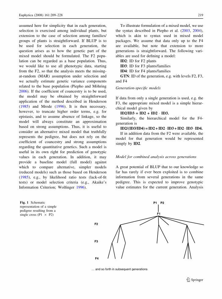
assumed here for simplicity that in each generation,

selection is exercised among individual plants, but

extension to the case of selection among families/

groups of plants is straightforward. If BLUP is to

be used for selection in each generation, the

question arises as to how the genetic part of the

mixed model should be formulated. The F2 popu-

lation can be regarded as a base population. Thus,

we would like to use all phenotypic data, starting

from the F2, so that the analysis meets the missing-

at-random (MAR) assumption under selection and

we actually estimate genetic variance components

related to the base population (Piepho and Mohring

2006). If the coefficient of coancestry is to be used,

the model may be obtained by straightforward

application of the method described in Henderson

(1985) and Mrode (1996). It is then necessary,

however, to truncate higher order terms, e.g. for

epistasis, and to assume absence of linkage, so the

model will always constitute an approximation

based on strong assumptions. Thus, it is useful to

consider an alternative mixed model that truthfully

represents the pedigree, but does not rely on the

coefficient of coancestry and strong assumptions

regarding the quantitative genetics. Such a model is

useful in its own right for prediction of genotypic

values in each generation. In addition, it may

provide a baseline model (full model) against

which to compare alternative, simpler models

(reduced models) such as those based on Henderson

(1985), e.g., by likelihood ratio tests (lack-of-fit

tests) or model selection criteria (e.g., Akaike’s

Information Criterion; Wolfinger 1996).

To illustrate formulation of a mixed model, we use

the syntax described in Piepho et al. (2003, 2004),

which is akin to syntax used in mixed model

packages. We assume that data only up to the F4

are available, but note that extension to more

generations is straightforward. The following vari-

ables are used for defining a model:

ID2: ID for F2 plants

ID3: ID for F3 plants/families

ID4: ID for F4 plants/families

GTN: ID of the generation, e.g. with levels F2, F3,

and F4

Generation-specific models

If data from only a single generation is used, e.g. the

F3, the appropriate mixed model is a simple hierar-

chical model given by

ID2/ID3 = ID2 + ID2 � ID3.

Similarly, the hierarchical model for the F4-

generation is

ID2/(ID3/ID4) = ID2 + ID2 � ID3 + ID2 � ID3 � ID4.

If in addition data from the F2 were available, the

model for that generation would be represented

simply by ID2.

Model for combined analysis across generations

A great potential of BLUP that to our knowledge so

far has rarely if ever been exploited is to combine

information from several generations in the same

pedigree. This is expected to improve genotypic

value estimates for the current generation. Analysis

P1 ×× P2

F1

… and so forth in subsequent generations

F4

F3

F2

Fig. 1 Schematic

representation of a simple

pedigree resulting from a

single cross (P1 · P2)

Euphytica (2008) 161:209–228 219

123

of data from multiple generations requires a joint

model that includes the generation (GNT) as a factor.

In all three generation-specific models, there is a

term ID2. Also, generation-specific models for F3 and

F4 have the term ID2 � ID3 in common. Despite this

notational identity, the effects in question cannot be

exactly the same over generations, as genotypes in

different generations are distinct due to meiotic events.

In order to formulate a single model over generations, it

is therefore necessary to introduce the factor GTN

coding different generations. Thus, the model could be

written GTN � ID2þGTN � ID2 � ID3þGTN � ID2�ID3 � ID4 There are two details that need to be

incorporated yet. Firstly, the effects GTN � ID2 � ID3

and GTN � ID2 � ID3 � ID4 do not appear in all

generations. Secondly, the effects are correlated across

generations. For example, GTN � ID2 represents the

effect of an F2-plant as operating in the F2 as well as in

the subsequent generations F3 and F4. The effects in

different generations corresponding to the same F2-

plant, while not identical, will be positively correlated.

This can be accommodated by regarding GTN as a

repeated factor and ID2 as the subject effect in repeated

measures terminology. In the notation of Piepho et al.

(2004) this is highlighted by writing the model as

GTN�ID2þGTN�ID2�ID3þGTN�ID2�ID3�ID4;

ð3Þ

where italizised terms are subject effects and non-

italizised effects are repeated effects (the model is

still not quite complete yet, as detailed below). Thus,

if u2, u3 and u4 represent the effect of an F2-plant as

operating in generations F2, F3 and F4, respectively,

modelled by GTN � ID2, we fit the model

varu2

u3

u4

0@

1A ¼ RF2: ð4Þ

Similarly, if v3 and v4 represent the effect of an F3-

plant or family in generations F3 and F4, respec-

tively, modelled by GTN � ID2 � ID3, we fit

varv3

v4

� �¼ RF3: ð5Þ

Finally, for consistency, the variance of an effect

w4 for the F4-families/individuals in the F4

generation, modelled by GTN � ID2 � ID3 � ID4,

is denoted as

var w4ð Þ ¼ RF4: ð6Þ

Model (3) does not yet correctly represent this

structure, because the factor GTN, appearing in all

three effects, has three levels, implying a 3-dimen-

sional covariance structure for each effect. This is in

contrast to structures (5) and (6), which have only

two and one dimension, respectively. Thus, GTN

needs to be replaced by terms specific to the different

effects. Depending on the mixed model package

being used, there are different ways of doing this. For

example, with SAS PROC MIXED it is convenient to

define the factors given in Table 1.

In Table 1, levels of a factor given in brackets

correspond to unobserved levels. They need to be set

equal to one of the observed levels (which one is

arbitrary!) so that the model can be fitted. Unob-

served levels will then be blocked out using dummy

variables as suggested in Piepho et al. (2006). The

dummies are defined in Table 2. With the definitions

in Tables 1 and 2, model (3) is modified as follows:

Z2�GTN2�ID2þ Z3�GTN3�ID2�ID3þZ4�GTN4�ID2�ID3�ID4: ð7Þ

Note that the dummy Z2 would not be strictly

needed, as its level is the same for all generations. It

Table 1 Definition of generation factors for repeated mixed

models representing a simple pedigree with phenotypic data

from several generations (Eq. 1)

Factor Levels Description

F2 F3 F4

GNT 2 3 4 Generation factor for F2 effects

GNT (3) 3 4 Generation factor for F3 effects

GNT (4) (4) 4 Generation factor for F4 effects

Table 2 Definition of dummy variables for repeated mixed

models representing a simple pedigree with phenotypic data

from several generations (model 1)

Dummy variable Levels Description

F2 F3 F4

Z2 1 1 1 Selector for F2 effects

Z3 0 1 1 Selector for F3 effects

Z4 0 0 1 Selector for F4 effects

220 Euphytica (2008) 161:209–228

123

is introduced simply for consistency with the other

effects, thus clarifying the model structure.

To complete the model, we also need to include a

fixed main effect for generations (GNT). As gener-

ation and year effects are confounded, this effect will

capture both year effects as well as true generation

effects due to inbreeding depression etc. For example,

with the definition of factors used here, assuming a

completely randomized design and homogeneity of

error variance for simplicity, specification of the

model in PROC MIXED of the SAS System is as

shown in Fig. 2. The corresponding code for ASReml

is given in Fig. 3. To illustrate the effect of shrinkage,

a small pedigree was simulated with 100 F2 plants, 5

F3 plants per F2 plant, and 4 F4 plants per F3 plant.

The simulation programme is available from the first

author upon request. Figure 4 shows a plot of

simulated BLUP, simulated BLUE and true geno-

typic values versus true values. The shrinkage of

BLUP compared to BLUE is clearly visible. The plot

also shows that BLUP is slightly biased downwards

for high true values, while it is biased upwards for

low true values. This bias, which is typical of BLUP,

is more than compensated for by the reduction in

variance. Consequently, the rank correlation of

simulated BLUP with true values (0.75) is higher

than that of simulated BLUE with true values (0.59).

It is perhaps useful here to point out that the meaning

of unbiasedness is different for BLUE and BLUP

(Searle et al. 1992). Unbiasedness for BLUE means

that E b� �

¼ b , while for BLUP unbiasedness relates

Table 3 Fits of two mixed models for factorial crosses of

maize (flint x dent) (Data kindly provided by T. Schrag, Uni-

versity of Hohenheim, Germany)

REML estimates

Covariance

parameter

With A &

DWithout A& D

Dent Var(per se) 17.36 33.12

Var(GCA) 18.18 22.03

Cov(GCA, per

se)

8.48 9.14

Flint Var(per se) 62.29 39.16

Var(GCA) 30.92 18.12

Cov(GCA, per

se)

7.67 2.76

Dent · Flint Var(SCA) 1.39 5.24

Log-likelihood

(REML):

�21721.4 �21656.6

-11-10

-9-8-7-6-5-4-3-2-10123456789

-6 -5 -4 -3 -2 -1 0 1 2 3 4 5

True value

BLUP/BLUE/True value

Fig. 4 Plot of simulated BLUP (black circles), BLUE (grey

dots), and true genetic values (solid line) versus true values

Fig. 2 SAS code for model (3)

Fig. 3 ASREML code for model (3).

Euphytica (2008) 161:209–228 221

123

to the fact that u and its BLUP have the same

expected values over the population, i.e.,

E uð Þ ¼ E uð Þ ¼ 0 . Note in particular that for BLUP

E uð Þ 6¼ u , which is commensurate with the type of

bias seen in Fig. 4.

It should be stressed that generation-specific and

genotype-by-environment effects are confounded.

There seems little one can do to dissect these effects,

unless several generations are planted in the same

trials, which is often impossible. If year main effects

are to be dissected from genotypic generation effects,

one needs to include standards, which would be

modelled as fixed effects. This can be done as

described in Piepho et al. (2006).

It may happen occasionally that the G matrix fitted

by REML is not positive-definite, particularly in

smaller datasets. In these cases, the mixed model

equations may be modified as suggested by Hender-

son (1984), and this option is implemented in PROC

MIXED. Also, the unstructured models for RF2 and

RF3 may be replaced by more parsimonious models

such as the factor-analytic model (Piepho 1997,

1998) or autoregressive models.

Discussion

This paper has reviewed the application of BLUP in

plant breeding both with and without pedigree

information. The use of pedigree information

requires defining a base population. There is no

absolute truth, however, concerning where we place

that base, though some choices are usually more

reasonable than others depending on the assump-

tions involved regarding the base population (link-

age phase equilibrium, Hardy–Weinberg

equilibrium, etc.) and the availability of complete

pedigree information. Assuming that current geno-

types are entirely uncorrelated might be taken as the

extreme choice, where we equate the base popula-

tion to the current set of genotypes. Alternatively,

when pedigree information is exploited, the base is

placed backwards in time to a point up to which all

ancestral relationships are known. To give an

example, consider a maize hybrid testing program

involving two heterotic pools. If we fit a model with

independent GCA and SCA effects, the base refers

to the current set of parental inbred lines, which are

then assumed unrelated. Alternatively, pedigree

information may be available back to the controlled

crosses between the most promising elite inbreds

used to develop the current parental inbred lines. In

this case, correlated GCA and SCA effects may be

modelled using the approach of Bernardo (1994).

The base would then correspond to the population of

initial founder inbreds, from which current parental

inbreds were derived. The fact that variance com-

ponent estimates differ whether or not pedigree

information is exploited does not necessarily imply

a bias. Differences must be expected because

variance components have different meaning, as

they refer to different base populations. Also, it

should perhaps be stressed that the assumption of

uncorrelated effects does not imply that we deny the

fact that the genotypes will always be related by

pedigree relative to some base population further

back in time.

In this paper we have contrasted BLUP based on

pedigree information derived from the coefficient of

coancestry and BLUP not using the coefficient of

coancestry. When the coefficient of coancestry is

used, it is possible to dissect different genetic effects

(additive, dominance, epistasis). This may be useful,

when only some of the genetic effects are easily

exploitable, as is the case in pedigree breeding with

self-pollinators, where mainly the additive genetic

effects are involved in response to selection. By

contrast, pedigree-based BLUP not using the coeffi-

cient of coancestry cannot discern additive and non-

additive genetic effect. It can, however, dissect

effects such as specific and general combining ability

(assuming these are not correlated by pedigree) as

well as within and between-family effects. Often the

main focus is merely on the estimation of the whole

genotypic value rather than on component genetic

effects comprising the genotype, so BLUP not using

the coefficient of coancestry is perfectly reasonable.

It is our belief that most of the time it is difficult to

give a strong justification for use of the coefficient of

coancestry based on quantitative-genetic theory,

because the full set of underlying statistical assump-

tions is difficult to fully meet or verify. In large

animal breeding programmes, where pedigree struc-

tures are extensive and complex, estimation of

genetic effects based on the coefficient of coancestry

making some strong simplifying assumptions often is

the only practical option. By contrast, many plant

breeding experiments give rise to fairly simple

222 Euphytica (2008) 161:209–228

123

hierarchical or crossed pedigree structures, for which

suitable mixed models can be derived from first

principles without taking recourse to a set of strong

assumptions based on quantitative-genetic theory

such as gametic-phase equilibrium, absence of epis-

tasis or selection, etc. The main assumption required,

when the coefficient of coancestry is not used, is that

genotypes in a reference generation, e.g. inbred

parents of a diallel or factorial experiment, can be

regarded as a random sample from some hypothetical

parent population. By ignoring the coefficient of

coancestry, we simply assume that all genotypes in

the reference generation are stochastically indepen-

dent. By contrast, when exploiting the coefficient of

coancestry, we go further back in time, tracing all

genotypes to a more distant base population were all

genotypes were unrelated. Thus, genotypes in the

current reference population become correlated by

pedigree. As a result, pedigree information is

exploited via genetic correlation. If we ignore the

pedigree, that information remains unutilized. Not

using the pedigree information relative to a hypo-

thetical, distant base population may be quite a

reasonable thing to do, however, when use of that

information would require unrealistic assumptions,

which one is not prepared to make.

That being said, we should also stress that, imper-

fections notwithstanding, use of the coefficient of

coancestry often does provide valuable information,

even when the usual quantitative-genetic assumptions

do not fully hold (Lynch and Walsh 1998, p. 793). We

believe that often the use of the coefficient of

coancestry can be motivated and justified heuristically

without taking recourse to strong assumptions about

the population genetic structure. For example, the

coefficient of coancestry may be regarded as a measure

of similarity, from which distances can be derived.

Thus, there is some analogy between BLUP based on

the A matrix, which makes predictions of genetic

effects based on genetic correlation with relatives, and

geostatistical methods such as Kriging, where local

predictions are made exploiting information from

neighboring observations based on spatial correlation

(Schabenberger and Gotway 2005). In fact, use of the

A and D matrix in case idealized assumptions of

quantitative-genetic theory do not hold may be justi-

fied to some degree by this analogy. Spatial methods

mainly require that spatial observations can be

regarded as a realization of a multivariate random

variable with covariance depending on spatial

distance. By analogy, one could assume that observed

genotypes constitute a realization of a multivariate

random variable with covariance depending on genetic

distance. This assumption does not require reference to

a specific base population with idealized properties.

All that is assumed is that genetic covariance depends

on genetic distance, while the specific form of this

dependence needs to be identified during the model-

building phase. For example, using principal coordi-

nate analysis (Digby and Kempton 1987), one might

consider finding a representation of genotypes in

Euclidean space, such that the implied distances are as

close as possible to those implied by the A matrix.

Then, a spatial model might be fitted to the principal

coordinates associated with the largest eigenvalues.

Use of the A matrix corresponds to the assumption that

genetic covariance shows a linear decay with genetic

distance. Alternatively, there are a large number of

non-linear models that might be explored, including

the exponential, power, and spherical models. For

these models there is no need of justification by

quantitative genetic theory, such as reference to an

idealized base population, except, perhaps, that use of

the coefficient of coancestry to define distance must be

justified. In addition, genetic distances may be

assessed based on marker data and distances can be

used in conjunction with geostatistical models in the

same way as the A matrix. Non-linear genetic covari-

ance structures may be further justified by the fact that

higher-order variance–covariance components (dom-

inance, additive · dominance, etc.) need to be ignored

and the coefficient of coancestry enters these compo-

nents in a non-linear way.

When marker data are used to infer genetic

relationships, such information may not be available

for all genotypes to be included in an analysis, while

complete pedigree data is available. In order to make

full use of the marker data, one might consider using

a compromise between the A matrix, as inferred from

the pedigree, and genetic similarity information as

assessed, e.g., by a similarity matrix S. Assume that A

is partitioned as

A ¼ A11 A12

A21 A22

� �; ð8Þ

such that A11 is the numerator relationship matrix for

the genotypes with marker information, while A22 is

Euphytica (2008) 161:209–228 223

123

the partition of A corresponding to genotypes without

marker information. The genetic variance–covariance

structure may then be modelled as

V¼ 0 A12

A21 A22

� �r2

A1þA11 0

0 0

� �r2

A2þS 0

0 0

� �r2

S:

ð9Þ

This structure allows finding the optimal compromise

among relationships from pedigree information (A11)

and marker information (S) for those genotypes with

information from both sources. The same idea can be

used when pedigree data is lacking for some geno-

types. When marker data is available for all geno-

types in addition to pedigree, one may consider

combining both sources in a similar fashion accord-

ing to V ¼ Ar2A þ Sr2

S . In all of these cases,

likelihood ratio tests (Oakay et al. 2006) or other

model selection criteria (Wolfinger 1996) may be

used to check which of the components of the genetic

variance–covariance structure is needed.

There is little literature on the robustness of BLUP

as used in plant breeding applications against depar-

ture from assumptions. Bernardo (1996c) found in a

simulation study that BLUP is robust when inbred

relationships are erroneously specified. Results from

the animal breeding literature indicate, however, that

biases may be substantial when information back to

the base population is not complete (Sorensen and

Kennedy 1984; Van der Werf & de Boer 1990; Dietl

et al. 1998; Schenkel et al. 2002; Jamrozik et al.

2007), and this was also found by Piepho and

Mohring (2006) in a plant breeding context. A

thorough investigation of robustness to mis-specified

pedigrees in diverse plant breeding settings is as yet

lacking. A further issue is robustness to non-normal-

ity. Departure from normality in the random effects is

rather difficult to detect (Verbeke and Lesaffre 1996;

Houseman et al. 2006). The fact that REML is

equivalent to iterated Minimum Norm Quadratic

Unbiased Estimation (I-MINQUE), which does not

require normality (Searle et al. 1992, p. 399), would

suggests that REML is robust to departures from

normality. Theoretical results show, however, that

inferences can be quite sensitive to departures from

normality, in particular in the presence of outliers

(Copt and Victoria-Feser 2006). Again, comprehen-

sive simulations with a focus on the plant breeding

context are as yet lacking.

The performance of BLUP depends crucially on

the availability of good variance estimates. In animal

breeding programmes there is often a very large

database for estimation of genetic variance compo-

nents. By contrast, plant breeding designs typically

yield a more limited number of genotypes. Also,

there may be heterogeneity of variance among

crosses, requiring cross-specific variance estimates

based on a small number of genotypes (White and

Hodge 1989, p. 295). In such cases, BLUP may

perform poorly when the genetic variance compo-

nents are not accurately estimated. An advantage of

the use of the coefficient of coancestry is that only a

single variance component needs to be estimated,

while all correlation is modelled via the A matrix. By

contrast, when the coefficient of coancestry is not

used, it is usually necessary to estimate several

variance components.

Heterogeneity of genetic variance components

among crosses could be tackled by a Bayesian

approach, by which estimation of the genetic variance

for a particular cross combines data from that cross

and from other crosses. In a plant breeding context,

this idea has been employed for estimating heteroge-

neous genotype-by-environment variance compo-

nents for assessing stability (Edwards and Jannink

2006). Generally, Bayesian methods are very com-

monly used in animal breeding (Gianola and Fer-

nando 1986), while applications in plant breeding so

far are relatively rare (see, e.g., Theobald et al. 2002).

When phenotypic data at the plot level are

available, it is preferable to perform a single-stage

analysis that accounts for all sources of variation. For

computational reasons, however, it may be necessary

to perform a two-stage analysis, where in the first

step, individual trials are analysed to compute

treatment means, which are then subjected to a mixed

model analysis over trials in the second stage. A

critical question in two-stage analyses is how to

optimally weight treatment means in the second

stage, based on the variance–covariance matrix of

trial-specific treatment means from stage one. That

matrix may be set equal to the residual variance–

covariance matrix R in the mixed model equations

(Eq. 1), when a model is formulated for means. Smith

et al. (2001a) propose to compute weights from the

diagonal elements of the inverse of R, arguing that

this inverse needs to be approximated in the mixed

model equations. Alternative weighting schemes are

224 Euphytica (2008) 161:209–228

123

possible, and a comparison of different options is

currently under way (Piepho and Mohring 2007).

Acknowledgements We thank J. Leon and A.M. Bauer for

critically reading an earler draft of this paper. Thanks are due

to Tobias Schrag for providing the maize data. We are grateful

to T. Calinski for helpful discussions on the spectral

decomposition of variance-covariance matrices. J. Mohring

was supported within the Breeding and Informatics (BRAIN)

project of the Genome Analysis of the Plant Biological System

(GABI) initiative (www.gabi.de). We thank all breeders of

GABI-BRAIN who have provided data and information on

their breeding programmes. Two anonymous referees are

thanked for very helpful comments.

References

Aleta N, Ninot A, Voltas J (2004) Retrospective evaluation of

parental selection in nursery tests of Juglans regia L. using

a mixed model analysis. Silvae Genet 53:26–33

Atlin GN, Baker RJ, McRae KB, Lu X (2000) Selection re-

sponse in subdivided target regions. Crop Sci 40:7–13

Bauer AM (2006) BLUP-Zuchtwertschatzung bei selbstbef-

ruchtenden Getreidearten unter Berucksichtigung aller

Verwandtschaftsinformationen und der In-

zuchtverhaltnisse. Diss, Bonn

Bauer AM, Reetz TC, Leon J (2006) Estimation of breeding

values of inbred lines using best linear unbiased predic-

tion (BLUP) and genetic similarities. Crop Sci 46:2685–

2691

Bernardo R (1993) Estimation of coefficient of coancestry

using molecular markers in maize. Theor Appl Genet

85:1055–1062

Bernardo R (1994) Prediction of maize single-cross perfor-

mance using RFLPs and information from related hybrids.

Crop Sci 34:20–25

Bernardo R (1995) Genetic models for predicting maize single-

cross performance in unbalanced yield trial data. Crop Sci

35:141–147

Bernardo R (1996a) Marker-based estimates of identity by

descent and alikeness in state among maize inbreds. Theor

Appl Genet 93:262–267

Bernardo R (1996b) Best linear unbiased prediction of maize

single-cross performance. Crop Sci 36:50–56

Bernardo R (1996c) Best linear unbiased prediction of the

performance of crosses between untested maize inbreds.

Crop Sci 36:872–876

Bernardo R (1999) Marker-assisted best linear unbiased pre-

diction of single-cross performance. Crop Sci 39:1277–

1282

Bromley CM, van Vleck LD, Johnson BE, Smith OS (2000)

Estimation of genetic variance from F1-performance with

and without pedigree relationships among inbred lines.

Crop Sci 40:651–655

Bueno JSD, Gilmour SG (2003) Planning incomplete block

experiments when treatments are genetically related.

Biometrics 59:375–381

Burgueno J, Crossa J, Cornelius PL, Trethowan R, McLaren G,

Krishnamachari A (2007) Modeling additive · environ-

ment and additive · additive · environment using ge-

netic covariance of relatives of wheat genotypes. Crop Sci

47:311–320

Calinski T, Czajka S, Kaczmarek Z, Krajewski P, Pilarczyk W

(2005) Analyzing multi-environment variety trials using

randomization-derived mixed models. Biometrics 61:448–

455

Cervantes-Matrinez CT, Frey KJ, White PJ, Wesenberg DM,

Holland JB (2001) Selection for greater b-glucan content

in oat grain. Crop Sci 41:1085–1091

Cervantes-Matrinez CT, Frey KJ, White PJ, Wesenberg DM,

Holland JB (2002) Correlated responses to selection for

greater b-glucan content in two oat populations. Crop Sci

42:730–738

Charcosset A, Bonnisseau B, Touchebeuf O, Burstin J, Dub-

reuil P, Barriere Y, Gallais A, Denis JB (1998) Prediction

of maize hybrid silage performance using marker data:

comparison of several models for specific combining

ability. Crop Sci 38:38–44

Chevalet C, Gillois M (1977) Estimation of genotypic variance

components with dominance in small consanguineous

populations. In: Pollak E, Kempthorne O, Bailey TB Jr

(eds), Proceedings of the International Conference on

Quantitative Genetics, August 16–21, 1976, Iowa State

University Press, Ames, pp 271–296

Cockerham CC (1954) An extension of the concept of partitioning

hereditary variance for analysis of covariances among rela-

tives when epistasis is present. Genetics 39:859–882

Cockerham CC, Weir BS (1984) Covariances of relatives

stemming from a population undergoing mixed self and

random mating. Biometrics 40:157–164

Colvin JA, Dykstra RL (1991) Maximum likelihood estimation

of a set of covariance matrices under Lowner order

restrictions with applications to balanced multivariate

variance components models. Ann Stat 19:850–869

Copas JB (1983) Regression, prediction and shrinkage. J Roy

Stat Soc B 45:311–354

Copt S, Victoria-Feser MP (2006) High-breakdown inference

for mixed linear models. J Am Stat Assoc 101:292–300

Cornelius PL, Crossa J, Seyedsadr MS (1996) Statistical tests

and estimators of multiplicative models for genotype-by-

environment data. In: Kang MS, Gauch HG Jr (eds)

Genotype-by-environment interaction. CRC Press, Boca

Raton, pp 199–234

Cornelius PL, Crossa J (1999) Prediction assessment of

shrinkage estimators of multiplicative models for multi-

environment cultivar trials. Crop Sci 39:998–1009

Crossa J, Burgueno J, Cornelius PL, McLaren G, Trethowan R,

Anitha K (2006) Modeling genotype x environmentinteraction using additive genetic covariances of relatives

for predicting breeding values of wheat genotypes. Crop

Sci 46:1722–1733

Cullis BR, Gogel BJ, Verbyla AP, Thompson R (1998) Spatial

analysis of multi-environment early generation trials.

Biometrics 54:1–18

Cullis BR, Lill WJ, Fisher JA, Read BJ (1989) A new proce-

dure for the analysis of early generation variety trials.

Appl Stat 2:361–375

Cullis BR, Smith A, Coombes N (2006) On the design of early

generation variety trials with correlated data. J Agr Biol

Environ Stat 11:381–393

Euphytica (2008) 161:209–228 225

123

Curnow RN (1980) Selecting crosses using information from a

diallel cross. Biometrics 36:1–8

Curnow RN (1988) The use of correlated information on

treatment effects when selecting the best treatment. Bio-

metrika 75:287–293

Da Costa RB, de Resende MDV, Goncalves PS, Silva MA

(2002) Individual multivariate REML/BLUP in the pres-

ence of genotype · environment interaction in rubber tree

(Hevea) breeding. Crop Breed Appl Biotechnol 2:131–

139

Davik J, Honne BI (2005) Genetic variance and breeding

values for resistance to a wind-borne disease [Sphaerot-heca macularis (Wallr. ex Fr.)] in strawberry (Fragaria ·ananassa Duch.) estimated by exploring mixed and spa-

tial models and pedigree information. Theor Appl Genet

111:256–264

De Boer IJM, Hoeschele I (1993) Genetic evaluation methods

for populations with dominance and inbreeding. Theor

Appl Genet 86:245–258

Dietl G, Wessely J, Rader I, Langhammer M (1998) Estimation

of genetic parameters for pigs based on crossbred off-

spring tested on farms. Achiv Anim Breed 41:291–298

Digby PGN, Kempton RA (1987) Multivariate analysis of

ecological communities. Chapman and Hall, London

Durel CE, Laurens F, Fouillet A, Lespinasse Y (1998) Utili-

zation of pedigree information to estimate genetic

parameters from large unbalanced data sets in apple.

Theor Appl Genet 96:1077–1085

Dutkowski GW, Costa e Silva J, Gilmour AR, Lopez GA

(2002) Spatial analysis methods for forest genetic trials.

Can J Forest Res 32:2201–2214

Eagles HA, Moody DB (2004) Using unbalanced data from a

barley breeding program to estimate gene effects: Ha2,

Ha4, and sdw1 genes. Aust J Agr Res 55:379–387

Edwards JW, Jannink JL (2006) Bayesian modeling of heter-

ogeneous error and genotype · environment interaction

variances. Crop Sci 46:820–833

Falconer DS, Mackay TFC (1996) An introduction to quanti-

tative genetics, 4th edn. Prentice Hall, London

Federer WT (1998) Recovery of interblock, intergradient, and

intervarietal information in incomplete block and lattice

rectangle designed experiments. Biometrics 54:471–481

Flachenecker C, Frisch M, Falke KC, Melchinger AE (2005)

Trends in population parameters and best linear unbiased

prediction of progeny performance in a European F2

maize population under modified recurrent full-sib selec-

tion. Theor Appl Genet 112:483–491

Frensham AB, Cullis BR, Verbyla AP (1997) Genotype by

environment variance heterogeneity in a two-stage anal-

ysis. Biometrics 53:1373–1383

Gallais A (1980) Is Fisher’s model necessary for the theory of

population improvement? Theor Appl Genet 58:177–180

Gauch HG (1988) Model selection and validation for yield

trials with interaction. Biometrics 44:705–715

Gianola D, Fernando RL (1986) Bayesian methods in animal

breeding theory. J Anim Sci 63:217–244

Gilmour AR, Cullis BR, Gogel B, Welham SJ, Thompson R

(2005) ASReml, user guide Release 2.0. VSN Interna-

tional Ltd, Hemel Hempstead

Goddard M (1986) Discussion summary Part VI: Selection and

non-random mating. In: Gianola D, Hammond K (eds)

Advances in statistical methods for genetic improvement

of lifestock. Springer, Berlin, pp 474–475

Henderson CR (1952) Specific and general combining ability.

In: Gowen JW (ed) Heterosis. Iowa State College Press,

Ames, pp 352–370

Henderson CR (1975) Best linear unbiased prediction under a

selection model. Biometrics 31:423–447

Henderson CR (1976) A simple method for computing the

inverse of a numerator relationship matrix used in the

prediction of breeding values. Biometrics 32:69–82

Henderson CR (1977) Prediction of the merits of single

crosses. Theor Appl Genet 49:273–282

Henderson CR (1984) Applications of linear models in animal

breeding. University of Guelph.

Henderson CR (1985) Best linear unbiased prediction of non-

additive genetic merits in non-inbred populations. J Anim

Sci 60:111–117

Henderson CR (1986) Statistical methods in animal improve-

ment: Historical Overview. In: Gianola D, Hammond K

(eds) Advances in statistical methods for genetic

improvement of lifestock. Springer, Berlin, pp 2–14

Henderson CR, Quaas RL (1976) Multiple trait evaluation

using relatives’ records. J Anim Sci 43:1188–1197

Hill RR Jr, Rosenberger JL (1985) Methods for combining

data from germplasm evaluation trials. Crop Sci 25:467–

470

Holland JB, Nyquist WE, Cervantes-Martinez CT (2003)

Estimating and interpreting heritability for plant breeding:

an update. Plant Breed Rev 22:9–112

Houseman EA, Coull BA, Ryan LM (2006) A functional-based

distribution diagnostic for a linear model with correlated

outcomes. Biometrika 93:911–926

Im S, Fernando RL, Gianola D (1989) Likelihood inferences in

animal breeding under selection: A missing-data theory

view point. Genet Sel Evol 21:399–414

James W, Stein C (1961) Estimation with quadratic loss. In:

Proc Fourth Berkeley Symp Math Statist Probab 1. Uni-

versity of California Press, Berkeley, pp 361–379

Jamrozik J, Fatehi J, Schaeffer LR (2007) Application of robust

procedures for estimation of breeding values in multiple-

trait random regression test-day model. J Anim Breed

Genet 124:3–11

Jannink JL, Bink MCAM, Jansen RC (2001) Using complex

plant pedigrees to map valuable genes. Trend Plant Sci

6:337–342

Jannink JL (2007) QTL by genetic background interaction.

Application to predicting progeny value. Euphytica (this

issue)

John JA, Williams ER (1995) Cyclic and computer generated

designs. Chapman and Hall, London

Lee Y, Nelder JA, Pawitan Y (2006) Generalized linear models

with random effects. Unified analysis via H-likelihood.

Chapman and Hall, London

Little RJA, Rubin DB (1987) Statistical analysis with incom-

plete data. Wiley, New York

Little RJA, Rubin DB (2002) Statistical analysis with incom-

plete data, Second edition. Wiley, New York

Lynch M, Walsh B (1998) Genetics and analysis of quantita-

tive traits. Sinauer, Sunderland

McCullagh P, Nelder JA (1989) Generalized linear models,

2nd edn. Chapman and Hall, London

226 Euphytica (2008) 161:209–228

123

Melchinger AE (1988) Means, variances, and covariances be-

tween relatives in hybrid populations with disequilibrium

in the parent populations. In: Weir BS, Eisen EJ, et al

(eds) Proc 2nd Int Conf Quantit Genet Raleigh, NC 31

May-5 June 1987, Sinauer Assoc, Sunderland MA, pp

400–415

Meuwissen THE, Luo Z (1992) Computing inbreeding coeffi-

cients in large populations. Genet Sel Evol 24:305–313

Miller A (2002) Subset selection in regression, 2nd edn.

Chapman and Hall, London

Moreno-Gonzalez J, Crossa J, Cornelius PL (2003) Additive

main effects and multiplicative interaction model: II.

Theory on shrinkage factors for predicting cell means.

Crop Sci 43:1976–1982

Moreno-Gonzalez J, Crossa J, Cornelius PL (2004) Genotype

· environment interaction in multi-environment trials

using shrinkage factors for ammi models. Euphytica

137:119–127

Mrode RA (1996) Linear models for the prediction of animal

breeding values. CAB International, Wallingford

Nyquist WE (1991) Estimation of heritability and prediction of

selection response in plant populations. Crit Rev Plant Sci

10:235–322

Oakey H, Verbyla A, Pitchford W, Cullis B, Kuchel H (2006)

Joint modelling of additive and non-additive genetic line

effects in single field trials. Theor Appl Genet 113:809–

819

Panter DM, Allen FL (1995a) Using best linear unbiased pre-

dictions to enhance breeding for yield in soybean. 1.

Choosing parents. Crop Sci 35:397–405

Panter DM, Allen FL (1995b) Using best linear unbiased

predictions to enhance breeding for yield in soybean. 2.

Selection of superior crosses from a limited number of

yield trials. Crop Sci 35:405–410

Pattee HE, Isleib TG, Gorbet DG, Giesbrecht FG, Cui Z (2001)

Parent selection in breeding for roasted peanut flavor

quality. Peanut Sci 28:51–58

Pattee HE, Isleib TG, Giesbrecht FG, Cui Z (2002) Prediction

of parental genetic compatibility to enhance flavor attri-

butes of peanuts. ACS Sym Ser 829:217–230

Patterson HD, Thompson R (1971) Recovery of inter-block

information when block sizes are unequal. Biometrika

58:545–554

Parisseaux B, Bernardo R (2004) In silico mapping of quan-

titative trait loci in maize. Theor Appl Genet 109:508–514

Persson T, Andersson B (2004) Accuracy of single- and mul-

tiple-trait REML evaluation of data including non-random

missing records. Silvae Genet 53:135–139

Piepho HP (1994) Best linear unbiased prediction (BLUP) for

regional yield trials: A comparison to additive main ef-

fects multiplicative interaction (AMMI) analysis. Theor

Appl Genet 89:647–654

Piepho HP (1997) Analyzing genotype-environment data by

mixed models with multiplicative effects. Biometrics

53:761–766

Piepho HP (1998) Empirical best linear unbiased prediction in

cultivar trials using factor analytic variance-covariance

structures. Theor Appl Genet 97:195–201

Piepho HP, Buchse A, Emrich K (2003) A hitchhiker’s guide to

the mixed model analysis of randomized experiments. J

Agron Crop Sci 189:310–322

Piepho HP, Buchse A, Richter C (2004) A mixed modelling

approach to randomized experiments with repeated mea-

sures. J Agron Crop Sci 190:230–247

Piepho HP, Mohring J (2005) Best linear unbiased prediction

for subdivided target regions. Crop Sci 45:1151–1159

Piepho HP, Mohring J (2006) Selection in cultivar trials—is it

ignorable? Crop Sci 146:193–202

Piepho HP, Mohring J (2007) On weighting in two-stage

analyses of series of experiments. Biuletyn Oceny Od-

mian (in press).

Piepho HP, Pillen K (2004) Mixed modelling for QTL ·environment interaction analysis. Euphytica 137:147–153

Piepho HP, Williams ER, Fleck M (2006) A note on the

analysis of designed experiments with complex treatment

structure. HortScience 41:446–452

Piepho HP, Williams ER (2006) A comparison of experimental

designs for selection in breeding trials with nested treat-

ment structure. Theor Appl Genet 113:1505–1513

Purba AR, Flori A, Baudouin L, Hamon S (2001) Prediction of

oil palm (Elaeis guineesis, Jacq.) agronomic performances

using best linear unbiased prediction (BLUP). Theor Appl

Genet 102:787–792

Reis AJS, Chaves LJ, Duarte JB, Brasil EM (2005) Prediction

of hybrid means from partial circulant diallel table using

the ordinary least square and the mixed model methods.

Genet Mol Biol 28:314–320

Resende RMS, Jank L, do Valle CB, Bonato ALV (2004)

Biometrical analysis and selection of tetraploid progenies

of Panicum maximum using mixed model methods. Pesqui

Agropecu Bras 39: 335–341

Robinson GK (1991) That BLUP is a good thing—the esti-

mation of random effects. Stat Sci 6:15–51

Rubin DB (1976) Inference and missing data. Biometrika

63:581–592

Santos AH, Bearoti E, Ferreira DF, da Silva Filho JL, (2002)

Simulation of mixed models in augmented block design.

Sci Agr 59:483–489

Schabenberger O, Gotway CA (2005) Statistical methods forspatial data analysis. CRC Press, Boca Raton

Schenkel FS, Schaeffer LR, Boettcher PJ (2002) Comparison

between estimation of breeding values and fixed effects

using Bayesian and empirical BLUP estimation under

selection on parents and missing pedigree information.

Genet Sel Evol 34:41–59

Schnell FW (1965) Die Covarianz zwischen Verwandten in

einer gen-orthogonalen Population. I. Allgemeine Theo-

rie. Biometr Z 7:1–49

Searle SR, Casella G, McCulloch CE (1992) Variance com-

ponents. Wiley, New York

Silva JCE, Wellendorf H, Borralho NMG (2000) Prediction of

breeding values and expected genetic gains in diameter

growth, wood density and spiral grain from parental selection

in Picea abies (L.) KARST. Silvae Genet 49:102–109

Simeao RM, Sturion JA, de Resende MDV, Fernandes JSC,

Neiverth DD, Ulbrich AL (2002) Avaliacao genetica em

erva-mate pelo procedimento BLUP individual multi-

variado sob interacao genotipo x ambiente. Pesqui Agro-

pecu Bras 37:1589–1596

Smith AB, Cullis BR, Gilmour AR (2001a) The analysis of

crop variety evaluation data in Australia. Aus N Z J Stat

43:129–145

Euphytica (2008) 161:209–228 227

123

Smith AB, Cullis BR, Thompson R (2001b) Analyzing variety

by environment trials using multiplicative mixed models

and adjustments for spatial field trend. Biometrics

57:1138–1147

Smith AB, Cullis BR, Thompson R (2005) The analysis of crop

cultivar breeding and evaluation trials: an overview of

current mixed model approaches. J Agr Sci 143:449–462

Sorensen D, Gianola D (2002) Likelihood, Bayesian, and

MCMC methods in quantitative genetics. Springer, Berlin

Sorensen DA, Kennedy BW (1984) Estimation of genetic

variances from unselected and selected populations. J

Anim Sci 59:1213–1223

Souza VAB, Byrne DH, Taylor JF (2000) Predicted breeding

values for nine plant and fruit characteristics of 28 peach

genotypes. J Am Soc Horticult Sci 125:460–465

Stroup WW, Mulitze DK (1991) Nearest neighbor adjusted

best linear unbiased prediction. Am Stat 45:194–200

Stuber CW, Cockerham CC (1966) Gene effects and variances

in hybrid populations. Genetics 54:1279–1286

Tancred SJ, Zeppa AG, Cooper M, Stringer JK (1995) Heri-

tability and patterns of inheritance of the ripening date of

apples. HortScience 30:325–328

Theobald CM, Talbot M, Nabugoomu F (2002) A Bayesian

approach to regional and local-area prediction from crop

variety trials. J Agr Biol Environ Stat 7:403–419

Thompson R (1973) The estimation of variance and covariance

components with an application when records are subject

to culling. Biometrics 29:527–550

Thompson R (1979) Sire evaluation. Biometrics 35:339–353

Van der Werf JHJ, de Boer IJM (1990) Estimation of additive

genetic variance when base populations are selected. J

Anim Sci 68:3124–2132

Verbeke G, Lesaffre E (1996) A linear mixed-effects model

with heterogeneity in the random-effects population. J Am

Stat Assoc 91:217–221

Viele K, Srinivasan C (2000) Parsimonious estimation of

multiplicative interaction in analysis of variance using

Kullback-Leibler Information. J Stat Plan Infer 84:201–

219

Wang DL, Zhu J, Li ZK, Paterson AH (1999) Mapping QTLs

with epistatic effects and QTL x environment interactions

by mixed linear model approaches. Theor Appl Genet

99:1255–1264

White TL, Hodge GR (1989) Predicting breeding values with

applications in forest tree improvement. Kluwer, Dordr-

echt

Wolfinger RD (1996) Heterogeneous variance-covariance

structures for repeated measures. J Agr Biol Environ Stat

1:205–230

Wricke G, Weber WE (1986) Quantitative genetics and

selection in plant breeding. De Gruyter, Berlin

Xiang B, Li BL (2001) A new mixed analytical method for

genetic analysis of diallel data. Can J Forest Res 31:2252–

2259

Xiang B, Li BL (2003) Best linear unbiased prediction of

clonal breeding values and genetic values from full-sib

mating designs. Can J Forest Res 33:2036–2043

Xu W, Virmani SS (2000) Prediction of hybrid performance in

rice: comparisons among best linear unbiased prediction

(BLUP) procedure, midparent value, and molecular mar-

ker distance. Int Rice Res Notes 25:12–13

Yan WK, Hunt LA, Johnson P, Stewart G, Lu X (2002) On-

farm strip trials vs. replicated performance trials for cul-

tivar evaluation. Crop Sci 42:385–392

Yan WK, Rajcan I (2003) Prediction of cultivar performance

based on single- versus multiple-year tests in soybean.

Crop Sci 43:549–555

Yu JM, Pressoir G, Briggs WH, Bi IV, Yamasaki M, Doebley

JF, McMullen MD, Gaut BS, Nielsen DM, Holland JB,

Kresovich S, Buckler ES (2006) A unified mixed-model

method for association mapping that accounts for multiple

levels of relatedness. Nat Genet 38:203–208

Zhang YM, Mao YC, Xie CQ, Smith H, Luo L, Xu SZ (2005)

Mapping quantitative trait loci using naturally occurring

genetic variance among commercial inbred lines of maize

(Zea mays L). Genetics 169:2267–2275

Zhu J, Weir BS (1994a) Analysis of cytoplasmatic and

maternal effects. I. A genetic model for diploid plant

seeds and animals. Theor Appl Genet 89:153–159

Zhu J, Weir BS (1994b) Analysis of cytoplasmatic and

maternal effects. II. Genetic models for triploid endo-

sperms. Theor Appl Genet 89:160–166

Zhu J, Weir BS (1996a) Diallel analysis for sex-linked and

maternal effects. Theor Appl Genet 92:1–9

Zhu J, Weir BS (1996b) Mixed model approaches for diallel

analysis based on a bio-model. Genet Res 68:233–240

228 Euphytica (2008) 161:209–228

123