arX

iv:n

ucl-

ex/0

6090

32 v

1 2

1 Se

p 20

06ANU/P 1678

Some notes on the program GKINT: Transient-field g-factor

kinematics at intermediate energies

Andrew E. Stuchbery

Department of Nuclear Physics, Australian National

University, Canberra, ACT 0200, Australia∗

(Dated: September 22, 2006)

Abstract

This report describes the computer program GKINT, which was developed to plan, analyze

and interpret the first High Velocity Transient Field (HVTF) g-factor measurements on radioac-

tive beams produced as fast fragments. The computer program and these notes were written in

September 2004. Minor corrections and updates have been added to these notes since then. The

experiment, NSCL experiment number 02020, Excited-state configurations in 38S and 40S through

transient-field g-factor measurements on fast fragments, was performed in October 2004; results

have been published in Physical Review Letters 96, 112503 (2006).

∗Tel. + 61 2 6125 2097, fax + 61 2 6125 0748, email:andrew.stuchbery@anu.edu.au

1

brought to you by COREView metadata, citation and similar papers at core.ac.uk

provided by CERN Document Server

xxxxxxxx

phoswich detectorAu/Fe target

magnetic field (out of page)Segmented Ge

γ-ray detector

40 MeV/Afragment beam

FIG. 1: Schematic view of the experimental arrangement viewed from above. Only the four SeGA

detectors perpendicular to the magnetic field axis are shown. There are ten other SeGA detectors

which are not shown for clarity.

I. INTRODUCTION

This report contains notes on the code GKINT. Much of the code was based on previous

programs for evaluating angular correlations and kinematics in transient-field g factor mea-

surements. These notes therefore tend to put an emphasis on the new features that have

been introduced into GKINT. Figure 1 shows the experimental arrangement that the code

is written to model.

II. OUTLINE OF THE PROGRAM GKINT

The code GKINT (G factor Kinematics at INTermediate energies) is based on previ-

ous codes written at ANU to evaluate the quantities of interest in transient-field g factor

measurements. The new features include (i) the use of relativistic kinematics (ii) Coulomb

excitation calculations of cross sections and angular correlation parameters appropriate for

intermediate energies.

2

The target can have up to 10 layers of compound composition. One layer has to be

specified as the ferromagnetic host. In the present version of the code, the ferromagnetic

layer is assumed to be Fe. Apart from the excitation of the 2+1 state of Fe, which is hard-

wired into the code, calculations can also be performed for any other ferromagnetic host. (If

the ferromagnet does not have Z = 26 this part of the calculation is skipped. At present the

intermediate energy code used is not a coupled-channels code. It cannot evaluate multiple

excitation, which might be needed for a valid calculation of the excitation of the rotational

Gd isotopes, even in glancing collisions.)

The main tasks performed by the code, in order, are:

1. Read in all input data.

2. Trace energy loss of beam through all target layers.

3. Calculate projectile Coulex and angular correlation parameters as a function of energy-

loss through the target at the average scattering angle.

4. Do detailed calculations of projectile Coulex cross sections, count rates, Doppler-

shift parameters, angular correlation parameters, transit times, ion energies/velocities

through each layer, transient-field precessions, etc., taking into account both the finite

solid angle of the particle counter and the energy loss of the beam in the target.

5. Evaluate angular correlations and perturbed angular correlations, including RIV ef-

fects, at the angles of the Segmented germanium array (SeGA).

6. Evaluate cross sections and angular correlations for excitation of the Fe target layer.

III. ENERGY LOSS

A. Energy loss algorithm

Energy loss of the beam in the target layers is evaluated using the stopping power for-

mulation of Ziegler et al. (1985). These stopping powers appear to be quite accurate for S

beams in Au and Fe targets. A provision is made to scale to stopping powers for each layer

by an input parameter.

3

Because the stopping powers are a function of energy, the energy loss calculations have

to be done by dividing the target layer into narrow strips of width ∆x. To work efficiently

with the thick foils that are used here, the energy loss algorithms were improved by using

the Runge-Kutta method.

To avoid confusing notation, we put dE/dx = S(E) to denote the energy dependence of

the stopping power. If the energy of the ion as it enters the strip n is En, then the energy

at the next strip En+1 is

En+1 = En − ∆E. (1)

We have to evaluate ∆E. The Runge-Kutta equations give

∆E = (∆E1 + 2∆E2 + 2∆E3 + ∆E4)/6 (2)

where

∆E1 = S(En)∆x (3)

∆E2 = S(En − ∆E1/2)∆x (4)

∆E3 = S(En − ∆E2/2)∆x (5)

∆E4 = S(En − ∆E3)∆x (6)

The Runge-Kutta method gives an exact solution (but for rounding errors) when S(E)

can be represented by a polynomial of degree not greater than four. Convergence is tested

by repeating the calculation with double the number of steps. The energy loss converges

within a few keV for targets several hundred mg/cm2 thick when a few hundred steps are

used. There can be a reduction in the accuracy if the ion almost stops, but such cases must

be avoided in an experiment anyway.

B. Energy loss calculations in GKINT

The first part of the calculation is to evaluate the energy loss of the beam through the

target layers. The beam energy at the front of each target layer is determined and the transit

time through the layer is evaluated. The energy with which the ion leaves the target is also

printed.

For the subsequent integrations, each target layer is then subdivided into a number of

strips of equal depth, and the energy of the beam at each strip is evaluated and stored. A

4

survey of the Coulomb excitation cross sections and angular correlation parameters (a2 and

a4) as a function of depth is made, assuming that the beam scatters at the average detection

angle, θ = (θmax + θmin)/2.

In the case of intermediate-energy fragments scattering at small angles, the difference

between the incident and scattered beam energies is very small. However it is evaluated pre-

cisely, and the subsequent energy loss of the scattered beam ion along its trajectory toward

the particle counter is evaluated as a function of depth through the target, as required.

IV. TRANSIENT-FIELD PRECESSIONS

Transient-field precessions are evaluated for ions that traverse the ferromagnetic layer of

the target using the routine ROTN. The primary purpose of this routine is to evaluate

φ(τ) = ∆θ/g = −µN

h

∫ Te

Ti

Btr(t)e−t/τ dt, (7)

where g and τ are the g factor and lifetime of the excited state. Btr is the transient-field

strength, which varies with time as the ion slows within the ferromagnet.

The integral over time is rewritten as an integral over energy using the non-relativistic

relations

dt = dx/v = dx/√

2E/M = dE√

M/2E/(dE/dx) (8)

where E is the energy and M is the mass of the ion. The use of the non relativistic formula

for energy is not expected to be too unrealistic because the TF strength is small until the

ion velocity falls to around 0.15c.

In the routine ROTN the integral over the energy range is performed using Simpson’s

rule. Along with the precession angle, ROTN evaluates a number of other quantities that

are often considered useful in relation to the Transient Field.

The effective time for which the ion experienced the TF during its flight through the

ferromagnetic foil layer must be evaluated first. From this, one may derive the average ion

velocity and the average TF strength.

If ti and te are the times at which the probe ion entered into and exited from the fer-

romagnetic foil, and τ is the mean life of the probe state, the effective interaction time

is

teff = τ [exp(−ti/τ) − exp(−te/τ)]. (9)

5

When τ ≫ ti, te,

teff = ti − te = tfe, (10)

where tfe is the time the probe ion takes to traverse the ferromagnetic layer. The average

velocity of the ion whilst in transit through the ferromagnet is

〈v/v0〉 = [∫ te

ti(v/v0) exp(−t/τ)dt]/teff , (11)

where v0 = c/137 is the Bohr velocity. Again, when the mean life is much longer than the

transit time,

〈v/v0〉 = L/[v0tfe], (12)

where L is the thickness of the ferromagnetic foil. If φ is expressed in milliradians and the

interaction time in ps, the average TF strength in kTesla is

〈BTF 〉 = 0.0209φ/teff . (13)

V. COULEX CALCULATIONS AND PARTICLE KINEMATICS

A. Modifications to COULINT

Coulex cross sections are evaluated using routines from COULINT, written by C.A.

Bertulani, see Phys. Rev. C 68, 044609 (2003). A few modifications were needed for the

present application.

Firstly, the COULINT routines were modified to return the CM differential cross section

for a specified energy and scattering angle. Both the Rutherford and Coulomb excitation

cross sections are returned. The code was also modified to return the statistical tensor

for the angular correlation in the projectile frame, at the specified energy and particle

scattering angle. Since there is some difference in the terminology, and in the definitions of

the statistical tensors, the code works with ak coefficients, which are the coefficients that

occur in the familiar Legendre polynomial expansion of the angular correlation:

W (θγ) = 1 + a2P2(cos θγ) + a4P4(cos θγ) (14)

The centre-of-mass to Lab transformations were evaluated with relativistic formulae:

tan θLab =1

γ2· sin θCM

(cos θCM + Mpγ1/Mtγ2)(15)

6

and

cos θCM =1

(1 + γ22 tan2 θLab)

−Mp

Mt

γ1γ2 tan2 θLab ±(

1 − M2p − M2

t

M2t

tan2 θLab

)1/2

(16)

where the positive sign is the only one relevant in the present work. The notation used here

drops the prime that in many references is attached to the factors γi. To define these gamma

factors it is convenient to introduce ρ = Mp/Mt. As usual we have

γ = (1 − v2/c2)−1/2 = 1 + T/m0c2 (17)

where T is the beam energy in MeV per nucleon and m0c2 = 931.494 MeV. In terms of ρ

and γ we have

γ1 =γ + ρ

(1 + 2ργ + ρ2)1/2(18)

and

γ2 =1 + γρ

(1 + 2ργ + ρ2)1/2(19)

The lab cross sections were evaluated as

dσLab

dΩLab

=dσCM

dΩCM

· dΩCM

dΩLab

(20)

The solid angle ratio, evaluated non-relativistically in terms of the particle scattering

angles, is

(dσ/dΩ)CM

(dσ/dΩ)Lab

=dΩLab

dΩCM

=

(

sin θLab

sin θCM

)2

| cos(θCM − θLab)| (21)

The relativistic formula is

dΩLab

dΩCM=

γ2[1 + (Mpγ1/Mtγ2) cos θCM]

[sin2 θCM + γ22(cos θCM + Mpγ1/Mtγ2)2]3/2

(22)

The code uses the proper relativistic evaluation, although the relativistic formulation

differs from the non-relativistic one by a negligible factor in many cases.

B. GKINT description: cross sections

Figures 2 and 3 show the variations in the projectile Coulomb excitation and Rutherford

cross sections as a function of scattering angle for 38S at 20 and 40 MeV/A, respectively,

incident on 197Au. The figures also show the excitation probability, Pi→f , which is

Pi→f =(dσ/dΩ)i→f

(dσ/dΩ)Rutherford(23)

7

cross sections at 20 MeV/A

38Scross section [fm /sr]

angle (degrees)0.0 1.0 2.0 3.0 4.0 5.0

-510

-410

-310

-210

-110

010

110

210

310

410

510

610

710

810

910

1010

Rutherford

Coulex

Excitation probablility

2

FIG. 2: Cross sections as a function of scattering angle for 20 MeV/A 38S on 197Au.

Note that the Rutherford cross section goes to infinity as the scattering angle approaches

zero. The Coulex cross section remains well behaved, however, because Pi→f approaches

zero faster than the Rutherford cross section diverges.

GKINT performs integrals over the solid angle of the particle detector and over the depth

of the target:

〈σ · ttgt〉 = 2π∫ ttgt

0

∫ θmaxp

θminp

dσ

dΩ(θp, E[z]) sin θpdθpdz, (24)

where the scattering angles and the cross section are in the lab frame, and z denotes the

depth through the target. With the cross sections in fm2 and target thickness in mg/cm2,

the count rate R in Hz is

R = Nbeam〈σ · ttgt〉NA

A(25)

8

cross sections at 40 MeV/A

38Scross section [fm /sr]

angle (degrees)0.0 1.0 2.0 3.0 4.0 5.0

-510

-410

-310

-210

-110

010

110

210

310

410

510

610

710

810

910

1010

Rutherford

Coulex

Excitation probablility

2

FIG. 3: Cross sections as a function of scattering angle for 40 MeV/A 38S on 197Au.

= (6.023 × 10−6)Nbeam〈σ · ttgt〉

A, (26)

where Nbeam is the number of beam ions/sec, NA is Avagadro’s number, and A is the

atomic mass number. The count rates for Coulomb excitation and Rutherford scattering

as registered by the particle counter are printed for Nbeam = 1000. If the Rutherford cross

section is in the region where it diverges and thus implies R > Nbeam, which is clearly

unphysical, the code puts R = Nbeam and prints a warning.

9

Scattering at 3 degrees lab angle

38S

a_2

beam energy [MeV]500 1000 1500

-0.5

0.0

0.5

FIG. 4: a2 angular correlation coefficient as a function of beam energy at a lab scattering angle of

3 for 38S on 197Au.

C. GKINT description: angular correlation coefficients

The spin alignment in intermediate energy Coulomb excitation depends on both the beam

energy and the scattering angle. As can be seen in Fig. 4, the alignment decreases as the

beam energy decreases, eventually changing sign. Similar behavior is evident when a2 is

plotted as a function of the scattering angle, Fig. 5. Again the alignment decreases with

scattering angle, eventually changing sign.

For each layer of the target, the average ak coefficients are evaluated as

〈ak〉 =2π

〈σ · ttgt〉∫ ttgt

0

∫ θmaxp

θminp

ak(θp, E[z])dσ

dΩ(θp, E[z]) sin θpdθpdz. (27)

The integrals are performed numerically using Simpson’s rule.

Similar integrals are performed to evaluate the average energy of excitation, the average

transient-field precessions, etc. In each case the quantity to be averaged replaces ak in an

expression of the same form as Eq. (27).

10

38S

a_2

lab scattering angle (degrees)0 1 2 3 4 5

-0.5

0.0

0.5

20 MeV/A

40.5 MeV/A

FIG. 5: a2 angular correlation coefficient as a function of lab scattering angle for 38S on 197Au.

VI. ANGULAR CORRELATION FORMALISM

The theoretical expression for the unperturbed angular correlation after Coulomb exci-

tation in general can be written as

W (θγ, φγ) =∑

k,q

√

(2k + 1)ρkq(θp, φp)FkGkQkDk∗q0 (φγ, θγ, 0), (28)

where ρkq(θp, φp) is the statistical tensor which defines the spin alignment of the initial

state, and depends on the particle scattering angles (θp, φp), Fk represents the usual F -

coefficients for the γ-ray transition, Gk is the vacuum deorientation attenuation factor,

Qk is the attenuation factor for the finite size of the γ-ray detector and Dkq0(φγ, θγ , 0) is

the rotation matrix, which depends on the γ-ray detection angles (θγ , φγ). The Coulex

calculation uses a right-handed co-ordinate frame in which the beam is along the positive

z-axis. In the applications of interest k = 0, 2, 4.

Since we are interested in the case where the particle detector has azimuthal symmetry,

the statistical tensors ρkq depend only on θp and are non-zero only when q = 0:

ρkq(θp, φp) = δq,0ρk0(θp) (29)

The program GKINT integrates the Coulex cross sections over the opening angle of the

11

particle detector and evaluates the ak coefficients defined as

ak =√

(2k + 1)ρk0Fk (30)

In the experiments a magnetic field will be applied in the vertical direction, along the

x-axis or φ = 0 direction. We define FIELD UP as being when the external field points UP

along the positive x-axis. The transient-field precession is given by

∆θ = gφ = −gµN

h

∫ Te

Ti

Btr(t)e−t/τ dt, (31)

where g is the nuclear g factor, τ is the meanlife of the level, and Ti and Te are the times at

which the ion enters into and exits from the ferromagnetic foil. (This expression corresponds

to the precession information in the whole gamma-ray lineshape, including decays which

occur while the nucleus is still in motion through the ferromagnet. The code also evaluates

the precession for those nuclei that decay in vacuum after leaving the ferromagnetic layer of

the target.) The important point to note here is that the precession angle, ∆θ, is negative

for a positive field (i.e. field UP) and a positive g factor.

Now consider that the nucleus undergoes a transient-field precession of ±∆θ as the ex-

ternal field is alternatively flipped up and down. We set aside the question of whether the

positive precession corresponds to field-up or field-down, since we don’t know the sign of the

g factor a priori. The statistical tensor is then modified by the precession about the field

axis, according to

ρkq(±∆θ) =∑

Q

ρkQδQ,0DkqQ(π/2,±∆θ,−π/2) (32)

= ρk0Dkq0(π/2,±∆θ, 0) (33)

= ρk0Dkq0(±π/2, |∆θ|, 0) (34)

= ρk0

√

4π

(2k + 1)Y k

q (|∆θ|,±π/2) (35)

In GKINT it is convenient to work with spherical harmonics rather than the rotation

matrices. To get the final form of the perturbed angular correlation we need to use

Dkq0(α, β, γ) =

√

4π

(2k + 1)Y k

q (β, α) (36)

and

Y k∗q (β, α) = (−1)qY k

−q(β, α) (37)

12

Note that, depending on the implementation in the computer routine, putting a negative β

value in the D matrix, and/or the spherical harmonic, may not be properly interpreted. We

will therefore avoid doing it in the code.

We then get the final expression for the perturbed angular correlation which GKINT

uses:

W (θγ, φγ,±∆θ) = 4π∑

k,q

akQkGk

(2k + 1)(−1)qY k

q (|∆θ|,±π/2)Y k−q(θγ , φγ) (38)

The evaluation of the vacuum deorientation parameters, Gk, is discussed below. At

present the gamma detector solid angle factors Qk are all set to unity. We will need to

formulate a procedure to evaluate these in future (perhaps using GEANT). However the

detectors are sufficiently far from the target that Qk = 1 is a reasonable first approximation.

VII. LORENTZ CORRECTION FOR γ RAYS

Because we have azimuthal symmetry, the Lorentz correction in this case is quite straight-

forward. The basic formulae, which have been written in many publications, are reviewed in

the first subsection. In the second subsection the method of treating the perturbed angular

correlation is discussed. I’m not aware of any place in the literature where this situation is

discussed in any detail.

A. Formulae for angular correlations

The angle between the beam axis and the direction of emission of the photon is affected

if the nucleus is in motion rather than at rest. The relativistic velocity addition formulae

can be used to show that the angles of emission in the laboratory, (θlab, φlab), are related to

those in the rest frame of the nucleus, (θnuc, φnuc), by the expressions

cos θlab =cos θnuc + β

1 + β cos θnuc

, (39)

and

φlab = φnuc, (40)

where β = v/c is the velocity of the nucleus along θlab = θnuc = 0. It follows that an element

of solid angle in the rest frame is related to an element of solid angle in the laboratory frame

13

by

dΩlab =1 − β2

(1 + β cos θnuc)2dΩnuc. (41)

To obtain the correlation in the laboratory frame, Wlab(θlab), from that in the rest frame of

the nucleus, Wnuc(θnuc), requires both transformation of the laboratory angle to the equiv-

alent angle in the rest frame of the nucleus using Eq. (39), and multiplication by the ap-

propriate solid-angle ratio so that the γ-ray flux emitted into 4π of solid angle is conserved,

i.e.∫

4πWlab(θlab)dΩlab =

∫

4πWnuc(θnuc)dΩnuc. (42)

This condition is satisfied if

Wlab(θlab) = Wnuc(θnuc)dΩnuc

dΩlab. (43)

B. Formulae for perturbed angular correlations

The precession of the nucleus takes place in the frame of the nucleus (obviously!). However

we measure the perturbed angular correlation in the Lab frame.

The standard technique for measuring small transient-field precessions in a way that

minimizes possible systematic errors is to form a double ratio of γ-ray intensities for each

complementary pair of γ-ray detectors placed at angles ±θγ with respect to the beam direc-

tion:

ρ =

√

√

√

√

N(+θγ↑)N(+θγ↓)

N(−θγ↓)N(−θγ↑)

, (44)

where N(±θγ ↑, ↓) denote the numbers of counts in the photopeak of the transition of interest

as registered in the detectors at ±θγ for the alternative field directions (↑ and ↓).The effect of the transient field is to rotate the angular correlation by a relatively small

angle around the direction of the applied magnetic field. Thus

W (θγ ↑) = W (θγ − ∆θ) ≃ W (θγ) − ∆θdW

dθ

∣

∣

∣

∣

∣

θγ

. (45)

In the case where there are no (or negligible) Lorentz effects, the precession angle ∆θ is

determined from

∆θ =ε

S, (46)

14

where

ε =1 − ρ

1 + ρ, (47)

and S, the logarithmic derivative of the angular correlation at the angle θγ , is

S =1

W

dW

dθ

∣

∣

∣

∣

∣

θγ

. (48)

To see how these expressions must be modified to account for Lorentz effects, it is con-

venient to note that ε is formally equivalent to

ε =W (+θγ↓) − W (+θγ↑)W (+θγ↓) + W (+θγ↑)

. (49)

The perturbed angular correlation in the lab frame is given by

Wlab(θlab ↑) = Wnuc(θnuc ↑)dΩnuc

dΩlab

= Wnuc(θnuc − ∆θ)dΩnuc

dΩlab

. (50)

Hence

εlab =W (θnuc↓) − W (θnuc↑)W (θnuc↓) + W (θnuc↑)

= εnuc. (51)

In the case of the Lorentz boost, the expression for ∆θ is

∆θ =εlab

Snuc

. (52)

Thus the only change in the analysis procedure is that S must be evaluated at the appropriate

angle in the rest frame of the nucleus, which corresponds to the laboratory detection angle.

Finally, it is worth noting that if W (θ) has the form of Eq. (14), then

S(θ) = −(a2P21(cos θ) + a4P41(cos θ))/W (θ) (53)

where P21 and P41 are associated Legendre polynomials.

VIII. RECOIL IN VACUUM ATTENUATION FACTORS

The Gk coefficients are evaluated as follows, based on experimental data and experience

at ANU.

For the experiments of interest, with ions emerging into vacuum with velocities near

the K-shell electron velocity, the vacuum deorientation is dominated by the fields at the

nucleus from the ground-state of the H-like electron configuration, i.e. 1s fields. At the

15

lower velocities of interest 2s fields also contribute. In this description, we will begin by

assuming that the 1s fields are dominant and then introduce the 2s contribution at the end.

The code uses both.

Neglecting the relativistic correction (which is small for Z = 16), the field at the nucleus

from the 1s electron of an H-like ion is

B1s = 16.7Z3 Tesla. (54)

This free-ion field causes the nuclear spin I to precess with a Larmor frequency of

ω = gµN

h(2I + 1)B1s (55)

The vacuum deorientation coefficients for a pure 1s configuration are

G1sk = 1 − bk

(ωτ)2

1 + (ωτ)2, (56)

where τ is the nuclear lifetime, and

bk = k(k + 1)/(2I + 1)2 (57)

Thus for I = 2 we have b2 = 0.24 and b4 = 0.80. In the worst case for I = 2, G1s2 (hardcore) =

0.76, and although G1s4 (hardcore) = 0.20, the k = 4 term (a4) in the angular correlation is

already small. In fact, for virtually any reasonable level lifetime (approaching a picosecond

or more) and a g-factor value that differs even a little from zero, the hyperfine field is so big

that G1sk ≈ G1s

k (hardcore).

We have measured the charge-state fractions for Si and S ions with energies between

about 90 MeV and 240 MeV emerging from Fe and Gd. (AES, Anna Wilson and Paul

Davidson, Nuclear Instruments and Methods B 243, 265 (2006).) The results for S after Fe

are shown in Fig. 6. Near v = Zv0 the 15+ charge state is dominant. The other prolific

charge states in their atomic ground states produce either smaller fields (13+) or no field at

all (14+ and 16+). Under these conditions it is reasonable to evaluate the average vacuum

deorientation coefficients for the experimental conditions in terms of the fraction of ions that

carry a single electron, QH . Thus

Gk = (1 − QH) + QHG1sk (58)

After some simple algebra we get

Gk = 1 − QHbk(ωτ)2

1 + (ωτ)2. (59)

16

32S after Fe

v/Z1v0

0.6 0.8 1.0 1.2

char

ge-s

tate

frac

tion

(%)

100

0.1

10

1

11+

14+ 15+

16+

13+

12+

FIG. 6: Charge-state fractions for S ions emerging from Fe as a function of the ion velocity. The

highest-velocity point was obtained with beams boosted by the ANU Linac. The curves are based

on fits to Eq. (62).

Thus provided that QH < 0.5, G2 > 0.88 and G4 > 0.6.

For S ions with velocities near 0.7Zv0 (100 MeV), the Li-like fields should be included:

Gk = 1 − QHbk(ωτ)2

1 + (ωτ)2− QLibk

(ωτ/8)2

1 + (ωτ/8)2(60)

where QLi is the lithium-like fraction, and it is assumed that

Bns = 16.7Z3/n3 Tesla. (61)

17

TABLE I: Results of fits to Eq. (62) for ions with 3 or fewer electrons.

Beam Target q v/Zv0 range Parameters

min max a0 a1 a2

Si Fe 14 0.83 1.26 -18.6231 26.2176 -9.6632

13 0.83 1.26 -9.6665 15.3430 -6.5868

12 0.83 1.26 -3.1681 7.0924 -4.8990

11 0.83 1.26 -4.1570 9.5851 -8.0001

S Fe: 16 0.67 1.08 -23.6376 36.5961 -14.9403

15 0.67 1.08 -14.9891 26.7520 -12.6089

14 0.67 1.08 -7.6139 15.9538 -9.3268

13 0.67 1.08 -3.1411 8.4963 -7.8757

S Gd 16 0.75 1.08 -17.8000 23.8431 -8.6552

15 0.64 1.08 -12.7697 20.9555 -9.2347

14 0.64 1.08 -6.0770 11.9903 -6.6953

13 0.64 1.08 -2.2632 5.3773 -5.1736

Si Gd 14 0.80 1.25 -17.9075 23.8099 -8.4427

13 0.80 1.25 -8.0397 11.4628 -4.4435

12 0.80 1.25 -5.6947 11.2019 -6.3201

11 0.80 1.12 0.5950 0.1204 -3.0000

The experimental data for the charge fractions in Fig. 6 were fitted to the form

F (q, v/Z1v0) = exp(a0 + a1v/Z1v0 + a2(v/Z1v0)2), (62)

where the parameters a0, a1 and a2 are determined for each charge state. The fit parameters

for the most prolific charge states are listed in Table I.

The code at present uses the fit to the charge-state results for S after Fe to interpolate

the values of QH and QLi and thus obtain as realistic an evaluation of Gk as possible. (It

18

will give a warning if the ion velocity is outside the region where there are experimental

data. The extrapolations must break down because the charge-state distributions are not

truly a gaussian function of ion velocity.)

The code uses the expression in Eq. (60) to evaluate the RIV effect. In the cases considered

to date, ωτ is so large that

(ωτ)2

1 + (ωτ)2≈ (ωτ/8)2

1 + (ωτ/8)2≈ 1, (63)

and hence, to an excellent approximation,

Gk = 1 − (QH + QLi)bk. (64)

Cautionary note: We know the form of G(t) for the vacuum deorientation effect, however

we measure

〈Gk〉 = (1/τ)∫

∞

texit

Gk(t) exp(−t/τ)dt, (65)

where texit is the time at which the ions emerge into vacuum. The code at present assumes

texit = 0 in the evaluation of the 〈Gk〉, as is the case for Eq. (56). This gives an accurate

result if texit ≪ τ . Thus the present calculations for 40S (τ ∼ 20 ps) should be fine, while

those for 38S (τ ∼ 5 ps) might tend to over estimate the vacuum deorientation effect slightly.

A more rigorous evaluation of the 〈Gk〉 value applicable in the experiments is available from

the Monte Carlo Doppler Broadened Line Shape (DBLS) code, GKINT MCDBLS.

IX. SOME PEDAGOGICAL PLOTS OF THE PERTURBED CORRELATIONS

A. TF precessions in the nuclear (projectile) frame

While the effect of the precession is most pronounced for detectors in the horizontal plane,

the other planes are also expected to show useful precession effects. The following figures

7 - 9 illustrate how the projectile (or nuclear frame) precession varies with the phi angle of

the γ-ray detector.

B. RIV perturbation in the lab frame

Fig. 10 shows the angular correlation in the lab frame with and without the RIV contri-

bution. In this case the particle scattering angle is between 2.5 and 5.5. The 38S beam

19

+/-100 mrad phi=90 deg

38S

W(theta)

theta [degrees]0 45 90 135 180

0.0

0.5

1.0

1.5

FIG. 7: Perturbed angular correlations in the CM frame as observed in the horizontal, or φ = 90,

plane.

+/-100 mrad phi=48 deg

38S

W(theta)

theta [degrees]0 45 90 135 180

0.0

0.5

1.0

1.5

FIG. 8: Perturbed angular correlations in the CM frame as observed in the φ = ±48 or φ = ±228

planes.

energy is 1540 MeV. The unattenuated angular correlation coefficients are a2 = −0.4233 and

a4 = −0.0990. For a H-like fraction of QH = 0.1269 and a Li-like fraction of QLi = 0.3108,

G2 = 0.8978 and G4 = 0.6595. The Lorentz effects are evaluated using β = 0.089.

Note that the RIV effect on the angular correlation is modest and that it is very difficult

to measure the RIV attenuation because γ-ray detectors cannot be placed at either 0 or 180

20

+/-100 mrad phi=37 deg

38S

W(theta)

theta [degrees]0 45 90 135 180

0.0

0.5

1.0

1.5

FIG. 9: Perturbed angular correlations in the CM frame as observed in the φ = ±37 or φ = ±217

planes.

to the beam in intermediate-energy Coulomb excitation measurements. The measurements

of the charge-state fractions are therefore very important.

X. FIGURE OF MERIT: OPTIMIZING EXPERIMENTAL CONDITIONS

GKINT provides the quantities designated S2W , S2N and S2φ2N evaluated at the SeGA

detector angles as figures of merit. This section explains the rationale of these choices as

figures of merit.

We begin by obtaining an estimate of the experimental error on the measured precession

for a given number of accumulated counts in a single pair of detectors. Since the precession

angles are relatively small, we can assume that

N(+θγ , ↑) ≈ N(−θγ , ↓) ≈ N(+θγ , ↓) ≈ N(−θγ , ↑) ≈ N. (66)

Thus N is the total number of counts recorded in one detector for one field direction. With

the further approximation that

σN ≈√

N, (67)

it follows that

σ∆θ ≈1

2S√

N.

21

with and without RIV contribution

38S

W(theta)

theta [degrees]0 45 90 135 180

0.0

0.5

1.0

1.5

FIG. 10: Angular correlation in the lab frame with and without the RIV contribution.

It is usually more convenient to work with a figure of merit that scales with the number of

counts, and hence is inversely proportional to the required beam time. Thus we can calculate

quantities proportional to S2N as the figure of merit and note that we must maximize it for

optimum sensitivity.

GKINT calculates both S2W and S2Wσ, denoting the latter as S2N . Generally S2N =

S2Wσ will be the quantity of interest. (S2W is retained in the output to give an indication

of the angular correlation contribution, separate from the cross section.) These figures of

merit are independent of the magnitude of ∆θ. Clearly, in a real experiment the goal is to

minimize σ∆θ/∆θ. As another figure of merit GKINT also evaluates

S2φ2Wσe(−Texit/τ), (68)

which is proportional to (σ∆θ/∆θ)2 for the fraction of excited nuclei that experience the full

transient-field precession and decay in vacuum beyond the target. Here Texit is the average

time at which beam ions exit from the target.

The calculations are given with and without the effect of the RIV attenuation. Since the

RIV effect can not be avoided, the unattenuated angular correlations are given mainly as a

point of reference.

22

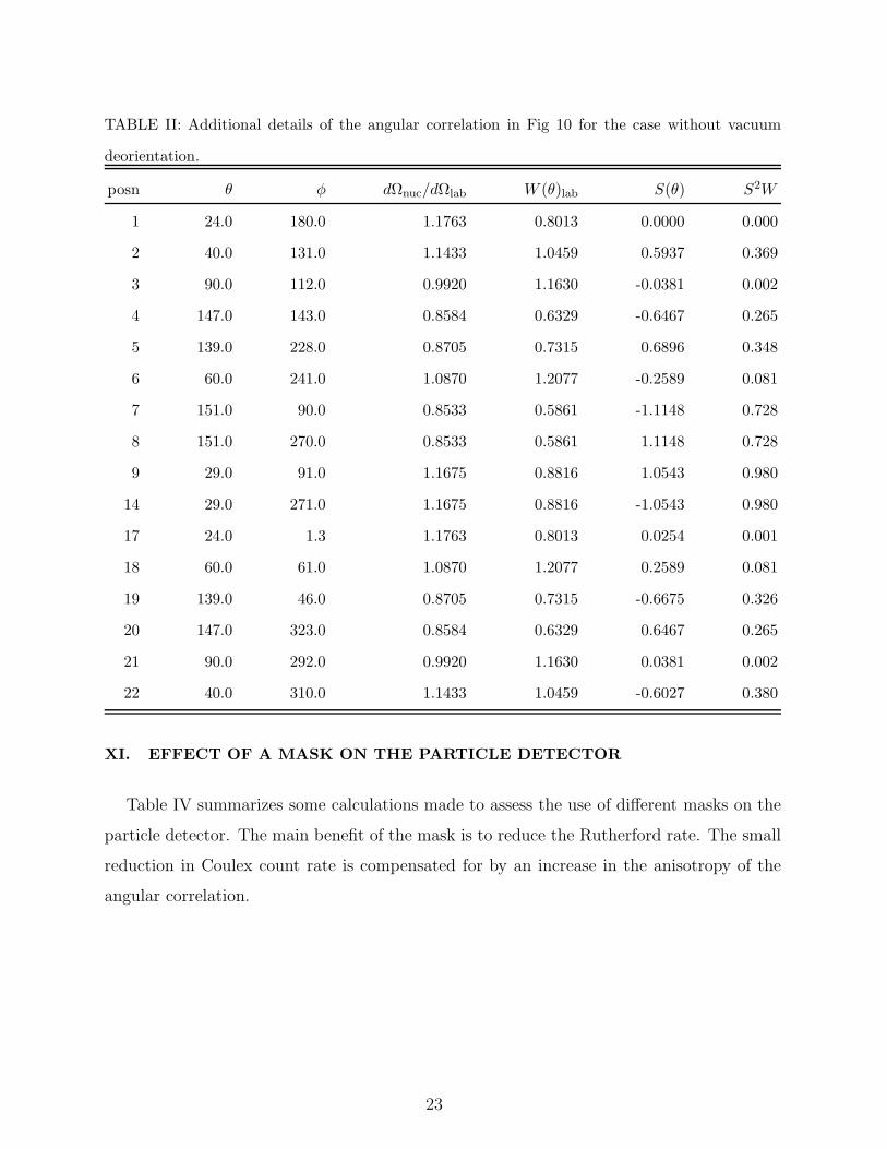
TABLE II: Additional details of the angular correlation in Fig 10 for the case without vacuum

deorientation.

posn θ φ dΩnuc/dΩlab W (θ)lab S(θ) S2W

1 24.0 180.0 1.1763 0.8013 0.0000 0.000

2 40.0 131.0 1.1433 1.0459 0.5937 0.369

3 90.0 112.0 0.9920 1.1630 -0.0381 0.002

4 147.0 143.0 0.8584 0.6329 -0.6467 0.265

5 139.0 228.0 0.8705 0.7315 0.6896 0.348

6 60.0 241.0 1.0870 1.2077 -0.2589 0.081

7 151.0 90.0 0.8533 0.5861 -1.1148 0.728

8 151.0 270.0 0.8533 0.5861 1.1148 0.728

9 29.0 91.0 1.1675 0.8816 1.0543 0.980

14 29.0 271.0 1.1675 0.8816 -1.0543 0.980

17 24.0 1.3 1.1763 0.8013 0.0254 0.001

18 60.0 61.0 1.0870 1.2077 0.2589 0.081

19 139.0 46.0 0.8705 0.7315 -0.6675 0.326

20 147.0 323.0 0.8584 0.6329 0.6467 0.265

21 90.0 292.0 0.9920 1.1630 0.0381 0.002

22 40.0 310.0 1.1433 1.0459 -0.6027 0.380

XI. EFFECT OF A MASK ON THE PARTICLE DETECTOR

Table IV summarizes some calculations made to assess the use of different masks on the

particle detector. The main benefit of the mask is to reduce the Rutherford rate. The small

reduction in Coulex count rate is compensated for by an increase in the anisotropy of the

angular correlation.

23

TABLE III: Additional details of the RIV attenuated angular correlation in Fig 10.

posn θ φ dΩnuc/dΩlab W (θ)lab S(θ) S2W

1 24.0 180.0 1.1763 0.8450 0.0000 0.000

2 40.0 131.0 1.1433 1.0454 0.5165 0.279

3 90.0 112.0 0.9920 1.1536 -0.0468 0.003

4 147.0 143.0 0.8584 0.6562 -0.5152 0.174

5 139.0 228.0 0.8705 0.7404 0.5773 0.247

6 60.0 241.0 1.0870 1.1911 -0.2669 0.085

7 151.0 90.0 0.8533 0.6169 -0.8662 0.463

8 151.0 270.0 0.8533 0.6169 0.8662 0.463

9 29.0 91.0 1.1675 0.9096 0.8472 0.653

14 29.0 271.0 1.1675 0.9096 -0.8472 0.653

17 24.0 1.3 1.1763 0.8450 0.0196 0.000

18 60.0 61.0 1.0870 1.1911 0.2669 0.085

19 139.0 46.0 0.8705 0.7404 -0.5588 0.231

20 147.0 323.0 0.8584 0.6562 0.5152 0.174

21 90.0 292.0 0.9920 1.1536 0.0468 0.003

22 40.0 310.0 1.1433 1.0454 -0.5242 0.287

24

TABLE IV: Effect of a mask on the particle detector. The calculations are for a standard 38S

configuration with Ebeam = 1540 MeV. The target is 355 mg/cm2 Au followed by 100 mg/cm2.

The stopping powers are scaled by a factor of 1.02.

θminp Count rate/1000 beam ions (Hz) S2Wσ

Coulex Rutherford

θmaxp = 5

0 0.0596 1000 762

1 0.0598 290 778

2 0.0523 63 856

2.5 0.0466 36 869

3 0.0395 21 836

θmaxp = 5.5

0 0.0720 1000 1119

1 0.0713 292 1138

2 0.0647 66 1236

2.5 0.0589 38 1260

3 0.0518 24 1237

25