Statistical Inference about Markov ChainsAuthor(s): T. W. Anderson and Leo A. GoodmanReviewed work(s):Source: The Annals of Mathematical Statistics, Vol. 28, No. 1 (Mar., 1957), pp. 89-110Published by: Institute of Mathematical StatisticsStable URL: http://www.jstor.org/stable/2237025 .Accessed: 24/05/2012 00:22

Your use of the JSTOR archive indicates your acceptance of the Terms & Conditions of Use, available at .http://www.jstor.org/page/info/about/policies/terms.jsp

JSTOR is a not-for-profit service that helps scholars, researchers, and students discover, use, and build upon a wide range ofcontent in a trusted digital archive. We use information technology and tools to increase productivity and facilitate new formsof scholarship. For more information about JSTOR, please contact support@jstor.org.

Institute of Mathematical Statistics is collaborating with JSTOR to digitize, preserve and extend access to TheAnnals of Mathematical Statistics.

http://www.jstor.org

STATISTICAL INFERENCE ABOUT MARKOV CHAINS

T. W. ANDERSON AND LEO A. GOODMAN1

Columbia University and University of Chicago Summary. Maximum likelihood estimates and their asymptotic distribution

are obtained for the transition probabilities in a Markov chain of arbitrary order when there are repeated observations of the chain. Likelihood ratio tests and x2-tests of the form used in contingency tables are obtained for testing the following hypotheses: (a) that the transition probabilities of a first order chain are constant, (b) that in case the transition probabilities are constant, they are specified numbers, and (c) that the process is a uth order Markov chain against the altemative it is rth but not uth order. In case u = 0 and r = 1, case (c) results in tests of the null hypothesis that observations at successive time points are statistically independent against the alternate hypothesis that observations are from a first order Markov chain. Tests of several other hypotheses are also considered. The statistical analysis in the case of a single observation of a long chain is also discussed. There is some discussion of the relation between likeli- hood ratio criteria and X2-tests of the form used in contingency tables.

1. Introduction. A Markov chain is sometimes a suitable probability model for certain time series in which the observation at a given time is the category into which an individual falls. The simplest Markov chain is that in which there are a finite number of states or categories and a finite number of equi- distant time points at which observations are made, the chain is of first-order, and the transition probabilities are the same for each time interval. Such a chain is described by the initial state and the set of transition probabilities; namely, the conditional probability of going into each state, given the im- mediately preceding state. We shall consider methods of statistical inference for this model when there are many observations in each of the initial states and the same set of transition probabilities operate. For example, one may wish to estimate the transition probabilities or test hypotheses about them. We de- velop an asymptotic theory for these methods of inference when the number of observations increases. We shall also consider methods of inference for more general models, for example, where the transition probabilities need not be the same for each time interval.

An illustration of the use of some of the statistical methods described herein has been given in detail [2]. The data for this illustration came from a "panel study" on vote intention. Preceding the 1940 presidential election each of a number of potential voters was asked his party or candidate preference each

Received August 29, 1955; revised October 18, 1956. 1 This work was carried out under the sponsorship of the Social Science Research Council,

The RAND Corporation, and the Statistics Branch, Office of Naval Research. 89

90 T. W. ANDERSON AND LEO A. GOODMAN

month from May to October (6 interviews). At each interview each person was classified as Republican, Democrat, or "Don't Know," the latter being a residual category consisting primarily of people who had not decided on a party or candidate. One of the null hypotheses in the study was that the probability of a voter's intention at one interview depended only on his intention at the im- mediately preceding interview (first-order case), that such a probability was constant over time (stationarity), and that the same probabilities hold for all individuals. It was of interest to see how the data conformed to this null hy- pothesis, and also in what specific ways the data differed from this hypothesis.

This present paper develops and extends the theory and the methods given in [1] and [2]. It also presents some newer methods, which were first mentioned in [9], that are somewhat different from those given in [1] and [2], and explains how to use both the old and new methods for dealing with more general hy- potheses. Some corrections of formulas appearing in [1] and [2] are also given in the present paper. An advantage of some of the new methods presented herein is that, for many users of these methods, their motivation and their application seem to be simpler.

The problem of the estimation of the transition probabilities, and of the test- ing of goodness of fit and the order of the chain has been studied by Bartlett [3] and Hoel [10] in the situation where only a single sequence of states is ob- ierved; they consider the asymptotic theory as the number of time points sncreases. We shall discuss this situation in Section 5 of the present paper, where a x2-test of the form used in contingency tables is given for a hypothesis that is a generalization of a hypothesis that was considered from the likelihood ratio point of view by Hoel [10].

In the present paper, we present both likelihood ratio criteria and X2-tests, and it is shown how these methods are related to some ordinary contingency table procedures. A discussion of the relation between likelihood ratio tests and x2-tests appears in the final section.

For further discussion of Markov chains, the reader is referred to [2] or [7].

2. Estimation of the parameters of a first-order Markov c.hain.

2.1. The model. Let the states be i = 1, 2, - - *, m. Though the state i is usually thought of as an integer running from 1 to m, no actual use is made of this ordered arrangement, so that i might be, for example, a political party, a geographical place, a pair of numbers (a, b), etc. Let the times of observation bet= 0,1,., T.Letpi,(t) (i,j= 1,... ,m;t = 1, --,T)betheproba- bility of state j at time t, given state i at time t - 1. We shall deal both with (a) stationary transition probabilities (that is, pij(t) = pij for t = 1, , T) and with (b) nonstationary transition probabilities (that is, where the transition probabilities need not be the same for each time interval), We assume in this section that there are ni(O) individuals in state i at t = 0. In this section, we treat the ni(O) as though they were nonrandom, while in Section 4, we shall discuss the case where they are random variables. An observation on a given

MARKOV CHAINS 91

individual consists of the sequence of states the individual is in at t = 0, 1, **, T, namely i(O), i(1), i(2), , i(T). Given the initial state i(O), there are m possible sequences. These represent mutually exclusive events with probabilities

(2.1) Pi(o)i(l) Pi(I)i(2) * Pi(T-1)i(T)

when the transition probabilities are stationary. (When the transition prob- abilities are not necessarily stationary, symbols of the form pi(t-_)i(t) should be replaced by pi(t-l)i(t) (t) throughout.)

Let nij(t) denote the number of individuals in state i at t- 1 and j at t. We shall show that the set of nij(t) (i, j = 1, , m; t = 1, , T), a set of m2T numbers, form a set of sufficient statistics fol the observed sequences. Let ni(o)i(i).. .i(T) be the number of individuals whose sequence of states is i(O), i(l), **-i(T). Then

(2.2) ngj(t) = ni(j) ... i (T)

where the sum is over all values of the i's with i(t -1) = g and i(t) = j. The probability, in the nmT dimensional space describing all sequences for all n individuals (for each initial state there are nT dimensions), of a given ordered set of sequences for the n individuals is

II [Pi(o)i(l) (1) pi()i(2) (2) - - - Pi(T-1)i(T)(T)]ni(O)i(1).*. i (T)

=J(I [pi(o) i(l)(1j)]ni(o) i t1) -i (T)) * * *([pi(T-1)ji(T) (T) ]ni ( ?) i ( 1).*.*. i ( T))

(2.3) = ( I pi(O),(.) (1)ni(o)i(j)(1)) . .. H II p,(,_,),(T) (T)n i(T- )i(T_ T i((.)3i(() i (T-1),i(T)

T

II TI pg, (t)noi(t) t=1 g,j

where the products in the first two lines are over all values of the T + 1 indices. Thus, the set of numbers nij(t) form a set of sufficient statistics, as announced.

The actual distribution of the nij(t) is (2.3) multiplied by an appropriate function of factorials. Let ni(t - 1) = Z=1 nij(t). Then the conditional distribution of nij(t), j = 1, , m, given ni(t -1) (or given nk(s), k = 1, m; s = O, *, t - 1) is

ni(t - 1)? " (2.4) m HII p ,(t)nii(t).

tI nij(t) ! j-' j=1

This is the same distribution as one would obtain if one had ni(t - 1) observa- tions on a multinomial distribution with probabilities pij(t) and with resulting numbers nij(t). The distribution of the nij(t) (conditional on the ni(O)) is

(2.5) ][ 1 (t)nii(t)___

nij(t)! 'JJ

92' T. W. ANDERSON AND LEO A. GOODMAN

For a Markov chain with stationary transition probabilities, a stronger result concerning sufficiency follows from (2.3); namely, the set nij = Et- nij(t) form a set of sufficient statistics. This follows from the fact that, when the transition probabilities are stationary, the probability (2.3) can be written in the form

T

(2.6) II II p;,vi(t) I p7i t-1 g.J i,

For not necessarily stationary transition probabilities pij(t), the nij(t) are a minimal set of sufficient statistics.

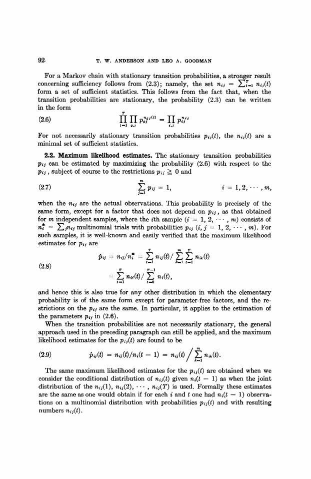
2.2. Maxium likelihood estimates. The stationary transition probabilities pij can be estimated by maximizing the probability (2.6) with respect to the pij, subject of course to the restrictions pj _ 0 and

m (2.7) E = 1, i = 1,2, ,m,

when the nif are the actual observations. This probability is precisely of the same form, except for a factor that does not depend on pij, as that obtained for m independent samples, where the ith sample (i = 1, 2, , m) consists of n* = EZnij multinomial trials with probabilities pij (i, j = 1, 2, m,). For such samples, it is well-known and easily verified that the maximum likelihood estimates for pij are

T m T

pij = En nij(t)/ E E nik(t)

(2.8) T tl kl- t-1

(2.8) ~ ~ ~~~~T T-1

E nii(t)/ E ni(t), tl1 t -o

and hence this is also true for any other distribution in which the elementary probability is of the same form except for parameter-free factors, and the re- strictions on the pij are the same. In particular, it applies to the estimation of the parameters pij in (2.6).

When the transition probabilities are not necessarily stationary, the general approach used in the preceding paragraph can still be applied, and the maximum likelihood estimates for the pij(t) are found to be

m (2.9) pij(t) = nq(t)/ni(t - 1) = nru(t)/ZE nk(t).

k-1

The same maximum likelihood estimates for the pij(t) are obtained when we consider the conditional distribution of n,j(t) given ni(t - 1) as when the joint distribution of the nmu(l), nij(2), * - , niu(T) is used. Formally these estimates are the same as one would obtain if for each i and t one had ni(t - 1) observa- tions on a multinomial distribution with probabilities pij(t) and with resulting numbers n j(t).

MARKOV CIAINS 93

The estimates can be described in the following way: Let the entries nfi(t) for given t be entered in a two-way m X m table. The estimate of pij(t) is the i, jth entry in the table divided by the sum of the entries in the ith row. In order to estimate piq for a stationary chain, add the corresponding entries in the two- way tables for t =1, **, T, obtaining a two-way table with entries nii - nij(t). The estimate of pii is the i, jth entry of the table of nij's divided by

the sum of the entries in the ith row. The covariance structure of the maximum likelihood estimates presented in

this section will be given further on.

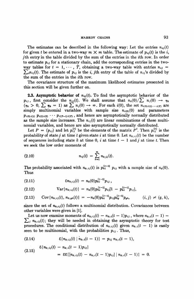
2.3. Asymptotic behavior of ni,(t). To find the asymptotic behavior of the p*, first consider the nij(t). We shall assume that nk(O)/Z nj(O) - lk

(fk > 0, EI Vk = 1) as E n3(O) -m oo. For each i(O), the set ni(o)j(l)... i(T) are simply multinomial variables with sample size nf(O) (0) and parameters Pi(O)i(i) Pi(l)i(2) ... pi(T-1)i(T) , and hence are asymptotically normally distributed as the sample size increases. The nij(t) are linear combinations of these multi- nomial variables, and hence are also asymptotically normally distributed.

Let P = (psi) and let p[t be the elements of the matrix Pt. Then ptt is the probability of state j at time t given state i at time 0. Let nkf; i,(t) be the number of sequences including state k at time 0, i at time t - 1 and j at time t. Then we seek the low order moments of

(2.10) n 2(t)- nk;i, (t)- k-I

The probability associated with nk;i (t) is Pki pij with a sample size of nk(O). Thus

(2.11) 6nk; j(t) = nk(0)pki pij,

(2.12) Var{nk; i(t) I nk(0)p "k1iPij[1 - P"ki-li j

(2.13) Cov{nk;jj(t), nk;,h(t) - -nk(0)p' pijpk9 P, (i, j) = (g, h),

since the set of nk;ij(t) follows a multinomial distribution. Covariances between other variables were given in [1].

Let us now examine moments of nk; i(t)- nk;i(t -l)pij, where nk;i(t - 1) Ej nk;ij(t); they will be needed in obtaining the asymptotic theory for test procedures. The conditional distribution of nk; ii(t) given nk; i(t - 1) is easily seen to be multinomial, with the probabilities pij. Thus,

(2.14) g{nk;ij(t) I nk;i(t - 1)) pt,j nk;i(t - 1),

(5 fnk;ij(t) - nk;i(t - 1)pi;I

- 8t[nk:ij(t) - nk;i(t - l)pij] I nk;i(t - 1) 0-.

99 T. W. ANDERSON AND LEO A. GOODMAN

The variance of this quantity is

8[fnk;ij(t) - nk;i(t - 1) pij]2

(2.16) = JI{[fnk;ji(t) - nk;i(t - 1) pij] I nk;i(t - 1)}

= &nk; ,(t - 1) pij(l - pij)

= nk(O) pk* ' pij(l - pi)

The covariances of pairs of such quantities are

8[nk;ij(t) - nk;i(t - 1) Pij][fk;ih(t) - nk;i(t - 1) Pih]

(2.17) = 881 [77k;ij(t) - nk;i(t - l)pij][nk;ih(t) - nk;i(t - l)PihJ I nk;i(t 1)}

=8[fnk;i(t - 1) Pii Pih] = -nk(O) pki t p*jpih ,j h,

8[fk;ij(t) - nk;i(t - l)Pij][fk;gh(t) - nk;g(t - 1) Pgh]

= 88&{ [k;ij(t) - nk;fi(t - l)Pi3j] [k;gh(t) - nk;g(t - l)PghI

I nk;i(t - 1), nk;g(t - 1)}

= O, ~~~~~~~~~~~i # q.

?[nk;ij(t) - nk;i(t - l)Pij][fk;gh(t + r) - nk;g(t + r - l)pg,]

=29 I[nk;ij(t) - nk;i(t - l)Pij]l[k;gh(t + r) - nk;g(t + 7 - l)Pgh]

( nk;g(t + r -1), nk; i(t -1), nk; ij(t)}

=0, r > 0.

To summarize, the randoin variables nk; ii(t) - nk; i(t - 1)pij for j = 1, m have means 0 and variances and covariances of multinomial variables with probabilities pij and sample size nk(0)pkit V'. The variables nk; j(t) - nk; i(t -1)p

and nk;gh(S) - nk;g(S - l)pgh are uncorrelated if t X s or i 5 g. Since we assume nk(O) fixed, nk;jj(t) and nl;gh(t) are independent if k X 1.

Thus

(2.20) 8[nij(t) - ni(t - 1)pij] = 0, m

(2.21) ? [nij(t) - ni(t - 1)pij]2 = "nk(0) pij(l - pij) ksl

8[n0j(t) - ni(t - 1)ptj][nh(t) -ni(t - 1)pih]

(2.22)--mj Znk(0)) pk Pij Pih, j 5 h, k=1

(2.23) &[nij(t) - n*(t - 1)pij][ngh(s) - ng(s - l)pgh] = 0, t X s or i z g.

MARKOV CHAINS 95

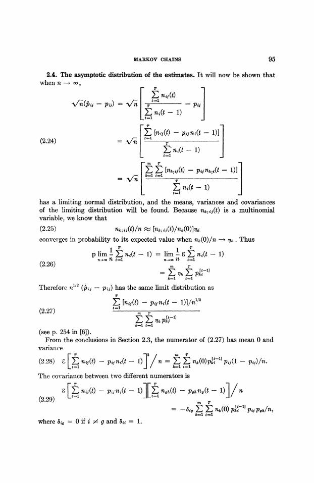
2.4. The asymptotic distribution of the estimates. It will now be shown that wheni n -oo

.r T

- p ij) = V-n T - pi

ni(t - 1)

-~ ~ ~~~ 1)] :?[nij(t) -pijni(t -1)]

(2.24) -=/n t

n(t - 1) _t=l m T

E j: [nk;ij(t) - pij nk.i(t - 1)]

_k-1 t-I - ,n - -

E ni(t -1)

has a limiting normal distribution, and the means, variances and covariances of the limiting distribution will be found. Because nk; ii(t) is a multinomial variable, we know that

(2.25) nk;ij(t)/n t~ [nk;ij(t)lnk(O)]qkr converges in probability to its expected value when nk(O)/n --. rn. Thus

T T

p lim -2E nf(t - 1) = lim - E nZ(t - 1) (2.26)

n >,o 71 t=1 noo nt t=l (2.26) n-~o r& fl~OOm T

= flk E pk$ k31 t=l

Therefore n'12 ( jj-pij) has the same limit distribution as T

, [nii(t) -pijni(t - 1)/nl/2 (2.27) t=i m

i E 7pt-1]

k=l1 t=1

(see p. 254 in [6]). From the conclusions in Section 2.3, the numerator of (2.27) has mean 0 and

variance T 2 m T

(2.28) E nii(t) - pini(t-1) /n = Z E nk(0)pkR-' pij(l - pj)/n. _ t31 _ ~~~~~~k=l t=l

The cov ariance between two different numerators is

f [i nii(t) - pin(t -1)][Z ngh(t) - phn(t-1) n (2.29) mtT

-bigE E n fk(0) pk I jpgh/n, k=i t=i

where Sg = 0 if i $ g and bii = 1.

96 T. W. ANDERSON AND LEO A. GOODMA N

Let m T

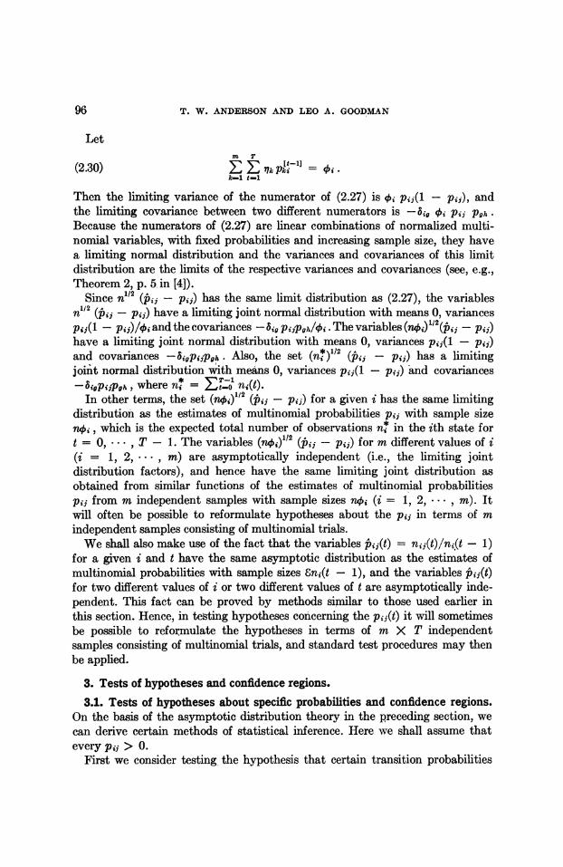
(2.30) E E7A vp[t-1] =

k-1 t -1

Then the limiting variance of the numerator of (2.27) is 4i pij(1 - pij), and the limiting covariance between two different numerators is -big qt pij pgh. Because the numerators of (2.27) are linear combinations of normalized multi- nomial variables, with fixed probabilities and increasing sample size, they have a limiting normal distribution and the variances and covariances of this limit distribution are the limits of the respective variances and covariances (see, e.g., Theorem 2, p. 5 in [4]).

Since n112 (Aij - jp) has the same limit distribution as (2.27), the variables n1/2 (ij - pij) have a limiting joint normal distribution with means 0, variances pi,(l1- pij)/4i and the covariances - igpit?pgh/Ai . The variables (n4i)"2(pij - pij)

have a limiting joint normal distribution with means 0, variances pij(l - pij) and covariances -bigpij-pgh. Also, the set (ni*)112 (i - pij) has a limiting joinit normal distribution with means 0, variances pij(l- pij) and covariances -5igpijPgh, where n* = ET-:0 ni(t).

In other terms, the set (n4i) 12 (Aij-ps) for a given i has the same limiting distribution as the estimates of multinomial probabilities pij with sample size n4i, which is the expected total number of observations n* in the ith state for t = 0, *. **, T -1. The variables (n4oi)112 (pij-pij) for m different values of i (i = 1, 2,*--, m) are asymptotically independent (i.e., the limiting joint distribution factors), and hence have the same limiting joint distribution as obtained from similar functions of the estimates of multinomial probabilities pij from m independent samples with sample sizes n4i (i = 1, 2, m). It will often be possible to reformulate hypotheses about the pij in terms of m independent samples consisting of multinomial trials.

We shall also make use of the fact that the variables pij(t) = nij(t)/ni(t -1) for a given i and t have the same asymptotic distribution as the estimates of multinomial probabilities with sample sizes 8ni(t - 1), and the variables jij(t) for two different values of i or two different values of t are asymptotically inde- pendent. This fact can be proved by methods similar to those used earlier in this section. Hence, in testing hypotheses concerning the pij(t) it will sometimes be possible to reformulate the hypotheses in terms of m X T independent samples consisting of multinomial trials, and standard test procedures may then be applied.

3. Tests of hypotheses and confidence regions. 3.1. Tests of hypotheses about specific probabilities and confidence regions.

On the basis of the asymptotic distribution theory in the preceding section, we can derive certain methods of statistical inference. Here we shall assume that every ps, > 0.

First we consider testing_ the hypothesis that certain transition probabilities

MARKOV CHAINS 97

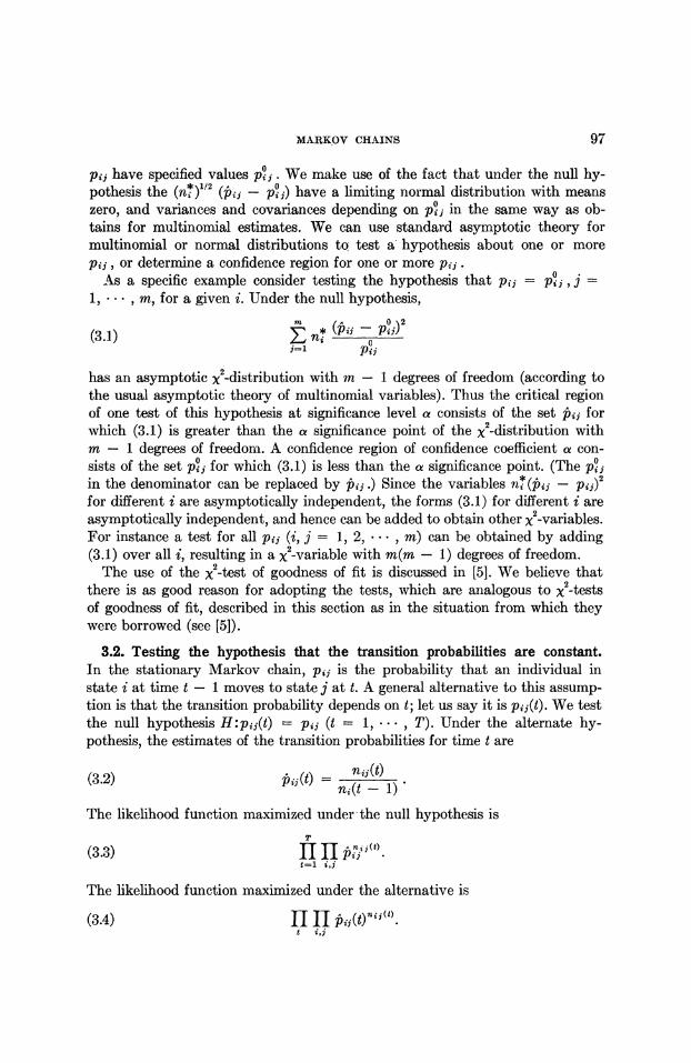
pij have specified values pi%. We make use of the fact that under the null hy- pothesis the (n*)112 (pijP- pIj) have a limiting normal distribution with means zero, and variances and covariances depending on pt in the same way as ob- tains for multinomial estimates. We can use standard asymptotic theory for multinomial or normal distributions to test a hypothesis about one or more pij, or determine a confidence region for one or more p,j.

As a specific example consider testing the hypothesis that pij - pSi,i 1,** , m, for a given i. Under the null hypothesis,

(3.1) n n* - J=i psi

has an asymptotic x2-distribution with m - 1 degrees of freedom (according to the usual asymptotic theory of multinomial variables). Thus the critical region of one test of this hypothesis at significance level a consists of the set pij for which (3.1) is greater than the a significance point of the x2-distribution with m - 1 degrees of freedom. A confidence region of confidence coefficient a con- sists of the set p?j for which (3.1) is less than the a significance point. (The po in the denominator can be replaced by pij.) Since the variables n4(jij 2

for different i are asymptotically independent, the forms (3.1) for different i are asymptotically independent, and hence can be added to obtain other X2-variables. For instance a test for all pij (i, j = 1, 2, ***, m) can be obtained by adding (3.1) over all i, resulting in a x2-variable with m(m - 1) degrees of freedom.

The use of the X2-test of goodness of fit is discussed in [5]. We believe that there is as good reason for adopting the tests, which are analogous to x2-tests of goodness of fit, described in this section as in the situation from which they were borrowed (see [5]).

3.2. Testing the hypothesis that the transition probabilities are constant. In the stationary Markov chain, pij is the probability that an individual in state i at time t - 1 moves to state j at t. A general alternative to this assump- tion is that the transition probability depends on t; let us say it is puj(t). We test the null hypothesis H:pij(t) = pij (t = 1, .- , T). Under the alternate hy- pothesis, the estimates of the transition probabilities for time t are

(3.2) nji(t) = (t) P ni (t -1)

The likelihood funietion maximized under' the null hypothesis is T

(3.3) TI nj ( t=l i,j

The likelihood function maximized under the alternative is

(3.4) TI I pij(t) t i,j

98 T. W. ANDERSON AND LEO A. GOODMAN

The ratio is the likelihood ratio criterion

(3.5) X II 11I [ I(

A slight extension of a theorem of Cram6r [61 or of Neyman [11] shows that -2 log X is distributed as x2 with (T - 1) [m(m - 1)1 degrees of freedom when the null hypothesis is true.

The likelihood ratio (3.5) resembles likelihood ratios obtained for standard tests of homogeneity in contingency tables (see [6], p. 445). We shall now de- velop further this similarity to usual procedures for contingency tables. A proof that the results obtained by this contingency table approach are asymptotically equivalent to those presented earlier in this section will be given in Section 6.

For a given i, the set Pij(t) has the same asymptotic distribution as the esti- mates of multinomial probabilities pij(t) for T independent samples. An m X T table, which has the same formal appearance as a contingency table, can be used to represent the joint estimates Pij(t) for a given - and for j = 1, 2, * *, m and t l 1 2,*- T.

t m2 m

1 p i (l) pi2(1) ... Pim(J)

2 pil (2) Pi2(2) ... jim(2)

T pil(T) pi2(T) ... pim(T)

The hypothesis of interest is that the random variables represented by the T rows have the same distribution, so that the data are homogeneous in this respect. This is equivalenit to the hypothesis that there are m constailts pil,

Pi2, * * with EZ pij = 1, such that the probability associated with the jth column is equal to pij in all T rows; that is, pij(t) = pij for t = 1, 2, * * , T. The %2-test of homogeneity seems appropriate here ([6], p. 445); that is, in order to test this hypothesis, we calculate

(3.6) xi = E ni(t - 1)[pij(t) P- ] / Pij t,j

if the null hypothesis is true, x% has the usual limiting distribution with (m - 1) (T - 1) degrees of freedom.

Another test of the hypothesis of homogeneity for T independent samples from multinomial trials can be obtained by use of the likelihood ratio criterion; that is, in order to test this hypothesis for the data given in the m X T table, calculate

Ai H [pij / Ai,(t)]nii j(t (3.7) = I[ p tJ

which is formally similar to the likelihood ratio criterion. The asymptotic distribution of -2 log Xi is x2 with (m - 1)(T - 1) degrees of freedom.

MARKOV CHAINS 99

The preceding remarks relating to the contingency table approach dealt with a given value of i. Hence, the hypothesis can be tested separately for each value of i.

Let us now consider the joint hypothesis that pij(t) = pij for all i 1, 2, **, m, j = 1, 2, ... , m, t = 1, - - *, T. A test of this joint null hypothesis follows directly from the fact that the random variables pij(t) and jij for two different values of i are asymptotically independent. Hence, under the null hypothesis, the set of x2 calculated for each i = 1, 2, * * , m are asymptotically independent, and the sum

(3.8) x Z x ni(t -1)[pij(t) - j / i=1 t t,j

has the usual limiting distribution with m(m - 1)(T - 1) degrees of freedom. Similarly, the test criterion based on (3.5) can be written

m

(3.9) E-2logXi= -2log X. i-1

3.3. Test of the hypothesis that the chain is of a given order. Consider first a second-order Markov chain. Given that an individual is in state i at t - 2 and in j at t - 1, let pijk(t) (i, j, k = 1, m , m; t = 2, 3, , T) be the probability of being in state k at t. When the second-order chain is stationary, pijk(t) -

pijk for t = 2, *--, T A first-order stationary chain is a special second-order chain, one for which pijk(t) does not depend on i. On the other hand, as is well- known, the second-order chain can be represented as a more complicated first- order chain (see, e.g. [2]). To do this, let the pair of successive states i and j define a composite state (i, j). Then the probability of the composite state (j, k) at t given the composite state (i, j) at t - 1 is pijk(t). Of course, the prob- ability of state (h, k), h $ j, given (i, j), is zero. The composite states are easily seen to form a chain with m2 states and with certain transition probabilities 0. This representation is useful because some of the results for first-order Markov chains can be carried over from Section 2.

Now let nijk(t) be the number of individuals in state i at t - 2, in j at t - 1, and in k at t, and let nij(t - 1) = Ek nijk(t). We assume in this section that the n,(O) and nij(l) are nonrandom, extending the idea of the earlier sections where the n.(O) were nonrandom and the nij(1) were random variables. The nijk(t) (i, j, k = 1, *-, m; t = 2, *.-, T) is a set of sufficient statistics for the different sequences of states. The conditional distribution of nijk(t), given nij(t- 1), is

(3.10) n ; (t) k 1)

(When the transition probabilities need not be the same for each time interval, the symbols pijk should, of course, be replaced by the appropriate pijk(t) through-

100 T. W. ANDERSON AND LEO A. GOODMAN

out). The joint distribution of nijk(t) for i, j, k = 1, , m and t = 2, *, T, when the set of nij(1) is given, is the product of (3.10) over i, j and t.

For chains with stationary transition probabilities, a stronger result concern- ing sufficiency can be obtained as it was for first-order chains; namely. the numbers n,jk = Et-2 nijk(t) form a set of sufficient statistics. The maximum likelihood estimate of Pijk for stationary chains is

m T T

(3.11) pijk= ijk= ni niJk(t)/ nir(t - 1). 1-1 t=2 t=2

Now let us consider testing the null hypothesis that the chain is first-order against the alternative that it is second-order. The null hypothesis is that Plik = P2ik Pmjk = pik. say, forj, k = 1,***, m. The likelihood ratio criterion for testing this hypothesis is2

(3.12) = (Pjk / ijk)'ik, i,j,k-l

where m m m T / T-1

(3.13) p= n i/ E E ni, = n njk(t)/ Z nj(t)

is the maximum likelihood estimate of pjk. We see here that pjk differs some- what from (2.8). This difference is due to the fact that in the earlier section the nij(l) were random variables while in this section we assumed that the n,j(l) were nonrandom. Under the null hypothesis, -2 log X has an asymptotic x2- distribution with m2(m - 1) - m(m - 1) = m(m - 1)2 degrees of freedom.

We observe that the likelihood ratio (3.12) resembles likelihood ratios ob- tained for problems relating to contingency tables. We shall now develop further this similarity to standard procedures for contingency tables.

For a given j, the n"12 (j. -Pijk) have the same asymptotic distribution as the estimates of multinomial probabilities for m independent samples (i = 1, 2, ... , m). An m X m table, which has the same formal appearance as a contingency table, can be used to represent the estimates pik for a given j and for i, k = 1, 2, * -, m. The null hypothesis is that pijk = Pik for i = 1, 2, ... , m, and the x2-test of homogeneity seems appropriate. To test this hy- pothesis, calculate

(3.14) Xi= E nIj(pijk - Pik) /Pjk i,k

where *T T T-1

(3.15) nf*j Z Enjk = E niik(t) = nj(t - 1) = E ni3(t). k k t=2 t-2 tlI

If the hypothesis is true, Xj has the usual limiting distribution with (m - 1)2 degrees of freedom.

2 The criterion (3.12) was written incorrectly in (6.35) of [1] and (4.10) of [2].

MARKOV CHAINS 101

In continued analogy with Section 3.2, aniother test of the hypothesis of homogeneity for m independent samples from multinomial trials canl be ob- tained by use of the likelihood ratio criterion. We calculate

(3.16) A 1. (=pik / Pijk)', i,k

which is formally similar to the likelihood ratio criteriotn. The asymptotic distributioni of -2 log X j is x2 with (m - 1)2 degrees of freedom.

The preceding remarks relating to the contingency table approach dealt with a given value of j. Hence, the hypothesis can be tested separately for each value of j.

Let us now consider the joint hypothesis that Pijk = Pik, for all i, j, k = 1, 2, , m. A test of this joint hypothesis can be obtained by computing the sum

n

(3.17) x x, Z ifjk p k - ) / PjkX j=1 j,i,k

which has the usual limiting distribution with m(m- 1)2 degrees of freedom. Similarly the test criterion based on (3.12) cani be written

E -2 log Xj = -2 log X = 2 E nijlog [ijk /jk] (3.18) ijk

= 2 E n ijk [log pijk - log pjk] ijk

The preceding remarks can be directly generalized for a chain of order r. Let Pij ..ki (i, j .** X k, 1 = 1, 2, ... m) denote the transition probability of state 1 at time t, given state k at time t- 1 ... and state j at time t - r + 1 and state i at time t - r (t = r, r + 1, * , T). We shall test the null hypothesis that the process is a chain of order r -1 (that is, pij. .ki = pi. ... k for i = 1, 2, * , m) against the alternate hypothesis that it is not an r -1 but an r-order chain.

Let n,..-.kl(t) denote the observed frequency of the states i, j, ***, k, 1 at the respective times t -r, t -.r + 1 , * s - I t, and let nii ... .k(t-1 El-, nif ... kl(t). We assume here that the niq.. .k(r- 1) are nonrandom. The maximum likelihood estimate of pij.. kl iS

(3.19) Pij... kl = nij - -kI/n, i - k

where ni,.. ki = Et-=r nij .. .kl(t) and TT-

(3.20) fl>...k = El... A- = E nj...k(t - 1) = (t) l t-r t-r-1

For a given set j, k , Ic, the set pij.. ik will have the same asymptotic distribu- tion as estimates of multinomial probabilities for m independent samples (i = 2, ..., m), and may be represented by an m X m table. If the null hypothesis

102 T. W. A NDEUcSON AND LEO A . GOODMAN

(Pj ..kl= pj * ki for i 1, 2, , m) is true, then the x2-test of homogeneity seems appropriate, and (3.21)

Xi-..k = Z. ..k(Pij .. kl - Pi ...k P... ki

i,l1 where

T ,T-1

(3.22) npj J...kl nWk/ Z j - E nnj,k(t)/ L f,... k(t),

i i t=r t=lr-l

has the usual limiting distribution with (m - 1)2 degrees of freedom. We see here that pj .- kl differs somewhat from the maximum likelihood estimate for pj.. -ki for an (r- 1)-order chain (viz., Zt=r- nj ... kl(t)/Zt=-r2 nf.. .k(t)). This difference is due to the fact that the njf.. .kz(r - 1), for an (r - 1)-order chain, are assumed to be multinomial random variables with parameters p. -kl while in this paragraph we have assumed that the nj... kl(r - 1) are fixed.

Since there are mr-1 sets j,**, k (j= 1, 2, *,m; k = 1, 2, , m), the sum Ej,. ..,k Xi E . will have the usual limiting distribution with mr1(rn _ 1)2 degrees of freedom under the joint null hypothesis (p,.j.kl = p-.. -kl for i = 1, 2, , m and all values from 1 to m ofj, , k) is true.

Another test of the null hypothesis can be obtained by use of the likelihood ratio criterion

(3.23) -1*j*k = II (iu..qcz/itj... lij k1 I i.l

where -2 log Xi.. k is distributed asymptotically as x2 with (m - 1)2 degrees of freedom. Also,

(3.24) E {-2 log X... k} = 2 n ij o ... kIg(jA.---kI/jA... kz)

j,- * . *,k i , j - *,k, I

has a limiting x2-distribution with mr1-(m- 1)2 degrees of freedom when the joint null hypothesis is true (see [10]).

In the special case where r 1, the test is of the null hypothesis that ob- servations at successive time points are statistically independent against the alternate hypothesis that observations are from a first-order chain.

The reader will note that the method used to test the null hypothesis that the process is a chain of order r - 1 against the alternate hypothesis that it is of order r can be generalized to test the null hypothesis that the process is of order u against the alternate hypothesis that it is of order r (u < r). By an ap- proach similar to that presented earlier in this section, we can compute the

2 x_-criterion or -2 times the logarithm of the likelihood ratio and observe that these statistic are distributed asymptotically as x2 with in7-mu](rn - 1) de- grees of freedom when the null hypothesis is true.

In this section, we have assumed that the transition probabilities are the same for each time interval, that is, stationary. It is possible to test the null hypothesis that the rth order chain has stationary transition probabilities

MARKOV CHA INS 103

using methods that are straightforward generalizations of the tests presented in the previous section for the special case of a first-order chain.

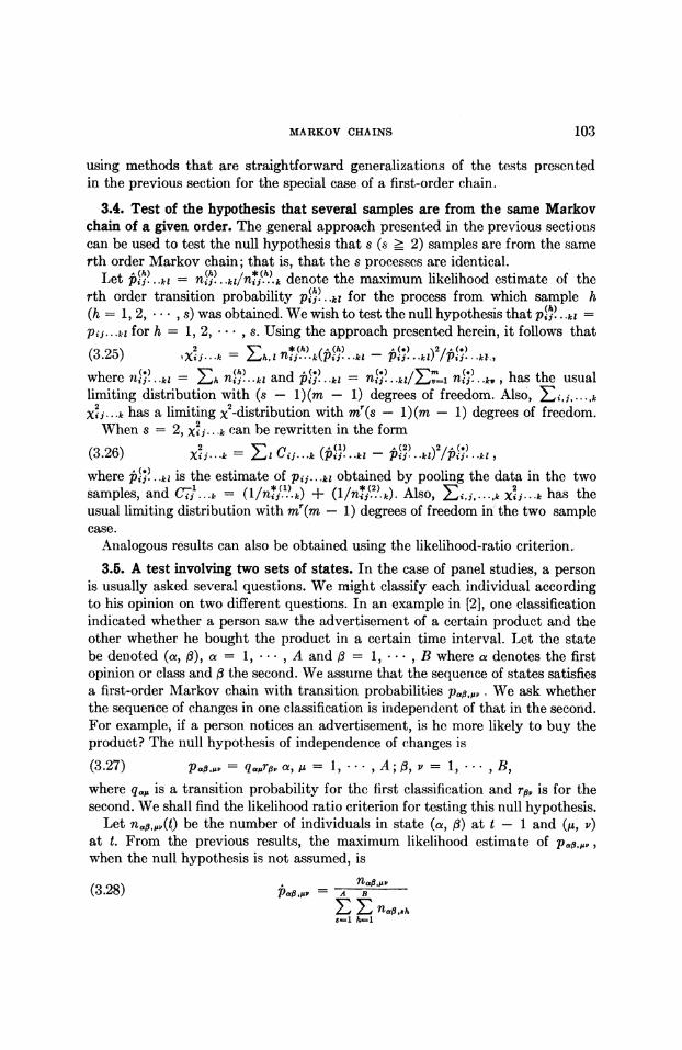
3.4. Test of the hypothesis that several samples are from the same Markov chain of a given order. The general approach presented in the previous sectiorns can be used to test the null hypothesis that s (s ? 2) samples are from the same rth order Markov chain; that is, that the s processes are identical.

Let p ..kl --= nj. ..ki/n, hk denote the maximum likelihood estimate of the rth order transition probability p(. ., for the process from which sample h (h = 1, 2, * * , s) was obtained. We wish to test the null hypothesis that p(h) ..k =

pij-.. k for h = 1, 2, , s. Using the approach presented herein, it follows that (3.25) 'Xti. k - -k iXl fhtl '(p(j) klh - P(; )2/jp()

where fl, ,. . .k = Eh r4, . . . k and px ? ..kl = n,; .,1k/Zv=.. n8? . .k,, has the usual limiting distribution with (s - l)(m - 1) degrees of freedom. Also, Ei,j. ..

Xii..k has a limiting x2-distribution with m7(s - )(m -1) degree.s of freedom. When s = 2, Xii. k can be rewritten in the form

(3.26) Xij,.-k E= I Cj.ic- (pIn ..-kl - P(j) .kl)/pi;. .1

where nj4?..kl is the estimate of pn. .1 obtained by pooling the data in the two samples, and :tib. . ik = (s/n - 1).k) ? (1/n, deg). Also, >Et,d,o. .,k - has the usual limiting distribution with m-(m -m1) degrees of freedom in the two sample case.

Analogous results can also be obtained using the likelihood-ratio criterion. 3.5. A test involving two sets of states. In the case of panel studies, a person

is usually asked se=eral questions. We might classify each individual according to his opinion on two different questions. In an example in [2], one classification indicated whe the es on saw the advertisement of a certain product and the other wahether he bought the product in a certain time interval. LJet the state besdenoteds(a,,),a- 1,*,Aandfl= 1,* , B where a denotes the first opinion or class and d3 the second. We assume that the sequence of states satisfies a first-order Markov chain with transition probabilities pE,,j.. WNe ask whether the sequence of ghanges in one classification is independent of that in the second. For example, if a person notices an advertisement, is he more likely to buy the product? The null hypothesis of independence of chanfges is

(3.27) uulak = quers ao s = 1m igh cl A; ,B, Y c= 1, ind *, B, where qah is a transition probability for the first classification and r is for the second. We shall find the likelihood ratio criterion for testing this null hypothesis.

Let nado ;(a) be the number of individuals in state (a, r) at td-1 and (t , v) at t. From the previous results, the maximum likelihood estimate of satisfi when the null hypothesis is not assumed, is

(3.28) pa,^ ,- = A B- I v . EEna#,.wh

(3.28 Pa.p A

104 T. W. ANDERSON AND LEO A. GOODMAN

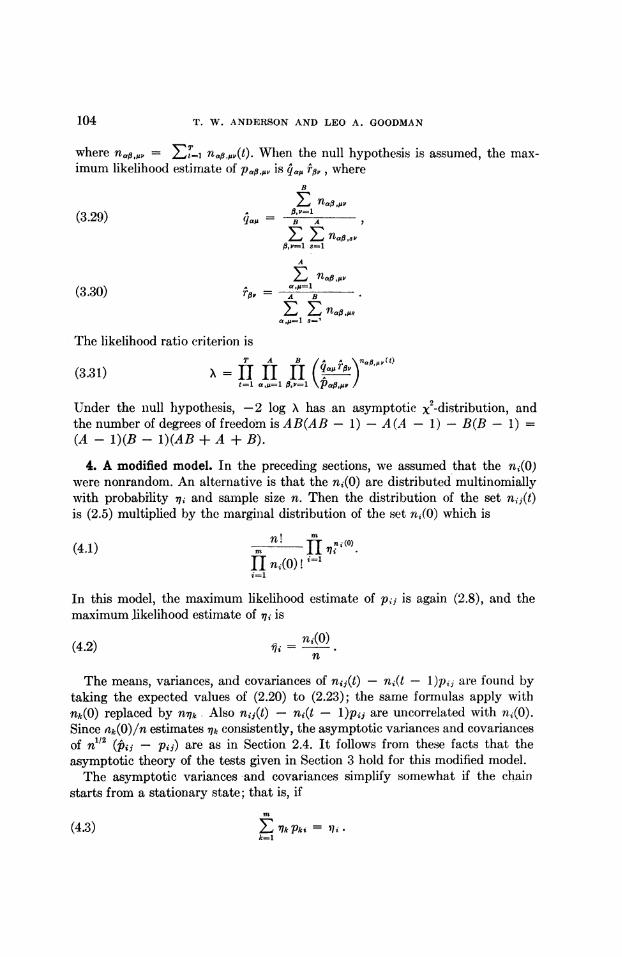
where nO, ,,> = ET=. nac,.4V(t). When the null hypothesis is assumed, the max- imum likelihood estimate of pa,#,,; is 'a r, , where

B

(3.29) A

~,v=1 s=l Eai B A#

A

(3.30) r A B

The likelihood ratio criterion is

(3.31) = A1 A

t = 1 a ,,u= 1 ;,t It1 pa#,A,

Under the null hypothesis, -2 log X has an asymptotic x2-distribution, and the number of degrees- of freedom is AB(AB - 1) -A (A - 1) - B(B - 1) = (A - 1)(B- 1)(AB + A + B).

4. A modified model. In the preceding sections, we assumed that the ni(O) were nonrandom. An alternative is that the ni(O) are distributed multinomially with probability ji and sample size n. Then the distribution of the set nij(t) is (2.5) multiplied by the marginal distribution of the set nJ(O) which is

(4.1) n II ni(0) ! i=l

In this model, the maximum likelihood estimate of pij is again (2.8), and the maximum.likelihood estimate of st is

(4.2) v ni(0) n

The means, variances, and covariances of nij(t) - njt - l)pij are found by taking the expected values of (2.20) to (2.23); the same formulas apply with nfk(O) replaced by nflfk Also nij(t) - ni(t - l)pij are uncorrelated with ni(O). Since nk(O)/n estimates flk consistently, the asymptotic variances and covariances of n112 ( ii- pii) are as in Section 2.4. It follows from these facts that the asymptotic theory of the tests given in Section 3 hold for this modified model.

The asymptotic variances -and covariances simplify somewhat if the chain starts from a stationary state; that is, if

(4.3) E k = Pk i . k=1

MARKOV CHAINS 105

For then E 'mk P "k-l - vi and Xi- T=i. If it is known that the chain starts from a stationary state, equations (4.3) should be of some additional use in the estimation of Pki when knowledge of the qi, or even estimates of the 77i, are available. We have dealt in this paper with the more general case where it is not known whether (4.3) holds, and have used the maximum likelihood esti- mates for this case. The estimates obtained for the more general case are not efficient in the special case of a chain in a stationary state because relevant information is ignored. In the special case, the maximum likelihood estimates for the 77j and pij are obtained by maximizing log L = Enij log puj + Eni(O) log vi subject to the restrictions ,/pij = 1, >2i 1pijP= ?i,j ?j= 1, pij ? 0, vi ? 0. In the case of a chain in a stationary state where the ?li are known, the maximum likelihood estimates for the pij are obtained by maximizing Enij log pij subject to the restrictions ,jpij = 1, Zi Nij = hj, pij > 0. Lagrange multipliers can be used to obtain the equations for the maximum

hood estimates.

5. One observation on a chain of great length. In the previous sections, asymptotic results were presented for ni(O) - oo, and hence Etl ni(O) - n -+ oo, while l' was fixed. The case of one observed sequence of states (n = 1) has been studied by Bartlett [3] and Hoel [10], and they consider the asymptotic theory when the number of times of observation increases (T -* oo). Bartlett has shown that the number nij of times that the observed sequence was in state i at time t - 1 and in state j at time t, for t = 1, I.. , T, is asymptotically normally distributed in the 'positively regular' situation (see [3], p. 91). He also has shown ([3], p. 93) that the maximum likelihood estimates pij = n,dn* (n* = Z>i nij) have asymptotic variances and covariances given by the usual multinomial formulas appropriate to 8 n* independent observations (i = 1, 2, * n, m) from multinomial probabilities pij (j = '1, 2, m , i), and that the asymptotic covariances for two different values of i are 0. An argument like that of Section 2.4 shows that the variables (n*)112 (j - pj) have a limiting normal distribution wvith means 0 and the variances and covariances given ir Section 2.4. This result was proved in a different way by IJ. A. Gardner [8].

Thus we see that the asymptotic theory for T -> oo and n = 1 is essentially the same as for T fixed and ni(O) - oo. Hence, the same test procedures are valid except for such tests as on possibly nonstationary chains. For example, Hoel's likelihood ratio criterion [10] to test the null hypothesis that the order of the chain is r - I against the alternate hypothesis that it is r is para,llel to the likelihood ratio criterion for this test given in Section 3.3. The x2-test for this hypothesis, and the generalizations of the tests to the case where the null hypothesis is that the process is of order u and the alternate hypothesis is that the process is of order r(u < r), which are presented in Section 3.3, are also applicable for large T. Also, the x2-test presented in Section 3.1 can be generalized to provide an alternative to Bartlett's likelihood ratio criterion [31 for testing the null hypothesis that pij...kl = pij... k (specified).

106 T. W. ANDERSON AND LEO A. GOODMAN

6. X2-tests and likelihood ratio criteria. The X2-tests presented in this paper are asymptotically equivalent, in a certain sense, to the corresponding likelihood ratio tests, as will be proved in this section. This fact does not seem to follow from the general theory of X2-tests; the X2-tests presented herein are different from those X2-tests that can be obtained directly by considering the number of individuals in each of the mT possible mutually exclusive sequences (see Section 2.1) as the multinomial variables of interest. The X2-tests based on mT categories need not consider the data as having been obtained from a Markov chain and the alternate hypothesis may be extremely general, while the X2-tests presented herein are based on a Markov chain model.

For small samples, not enough data has been accumulated to decide which tests are to be preferred (see comments in [5]). The relative rate of approach to the asymptotic distributions and the relative power of the tests for small samples is not known. In this section, a method somewhat related to the rela- tive power will be tentatively suggested for deciding which tests are to be pre- ferred when the sample size is moderately large and there is a specific alternate hypothesis. An advantage of the X2-tests, which are of the form used in con- tingency tables, is that, for many users of these methods, their motivation and their application seem to be simpler.

We shall now prove that the likelihood ratio and the X2-tests (tests of ho- mogeneity) presented in Section 3.2 are asymptotically equivalent in a certain sense. First, we shall show that the X2-statistic has an asymptotic X2-distribution under the null hypothesis. The method of proof can be used whenever the relevant p's have the appropriate limiting normal distribution. In particular, this will be true for statistics of the form x% (see (3.6)). In order to prove that statistics of the form Xi (see (3.7)), which are formally similar to the likelihood ratio criterion but are not actually likelihood ratios, have the appropriate asymptotic distribution, we shall then show that -2 log Xi is asymptotically -equivalent to the X%-statistic, and therefore it has an asymptotic X2-distribution under the null hypothesis. Then we shall discuss the question of the equiva- lence of the tests under the alternate hypothesis. The method of proof presented here can be applied to the appropriate statistics given in the other sections herein, and also where T -X as well as where n - oo.

Let us consider the distribution of the x2-statistic (3.8) under the null hy- pothesis. From Section 2.4, we see that n'12 (pij(t) - pij) are asymptotically normally distributed with means 0 and variances pij(1 - pij)/mi(t - 1), etc., where mi(t) = Sni(t)/n. For different t or different i, they are asymptotically independent. Then the [nmi(t- 1)]1I2 [k,j(t) - p,j] have asymptotically vari- ances pij(l - pij), etc. Let tjMM = E m (t- 1) pij(t)/ m;(t- 1). Then by the usual x2-theory, Enmi (t - A)[ ij(t) - p*j]2/ jA has an asymptotic x2-distribution under the null hypothesis. But

(6.1) P lim (j - j) 0

MARKOV CHAINS 107

because

(6.2) p lim (niM) )-miQ)) O.

From the convergence in probability of (pj4 p ij) and (mi(t) - ni(t)/n), and the fact that n'/2 (ij(t) - pij) has a limiting distribution, it follows that

(6.3) p lim nE mi(t -1)(P,(t) p-,) E

ni(t - i)(jp ,(t) O .u)] O Puj )ij

Hence, the X2-statistic has the same asymptotic distribution as ,nm,(t- 1) [Aij(t) _ A4'j]2/j4j; that is, a x2-distribution. This proof also indicates that the Xi-statistics (3.6) also have a limiting X2-distribution. We shall now show that -2 log Xi (see (3.7)) is asymptotically equivalent to x% under the null hypothesis; and hence will also have a limiting x2-distribution.

We first note that for {xl < a

(6.4) (1 + x) log (1 + x) = (1 + x)(x-x2/2 + 3/3 -x4/4+ *-)

= x + x2/2 - (2/6)(1 - x/2 + and

(6.5) (1 + x) log (1 + x) - x - x2/21 = (x/6)(1 - x/2 + )? _ Ix3I (see p. 217 in [6]). We see also that

-2 log Xi = -2 E ni1(t) log [ki/p j(t)] j,t

(6.6) = 2 E ni(t - 1) Apij(t) log [PAij(t)/jAi] j t

= 2 E ni(t - 1) A ij[1 + xij(t)] log [1 + xij(t)],

j,t

.where xij(t) = [ij(t) -_ iI/Aij . The difference A between -2 log X) and the xi-statistic is

A = -2 log Xi-x

= 2 Zj,t ni(t - l)Aij{ [1 + xij(t)] log [1 + xij(t)] - [xij(t)]2/21.

Since Z=1 A ijxij(t) = 0,

(6.8 /A = 2 E ni(t - l)Ai{ij [1 + xij(t)] log [1 + xij(t)] -xij(t) _ [xij(t)]2/21. j,t We shall show that A converges to 0 in probability; i.e. for any e > 0, the

probability of the relation I A I < c, under the null hypothesis, tends to unity as n = i ni(t) -m o. The probability satisfies the relation

Pr{ I A I < e} ? Pr{ I A I < e and I xij(t) I < 2} (6.9) > Pr{ 1 2 Ej,t ni(t- 1)pi[xij(t)]3 I< and I xi(t)I <-}

> Pr{2n Ej,t I xij(t) I" < e and I xij(t) I < I}.

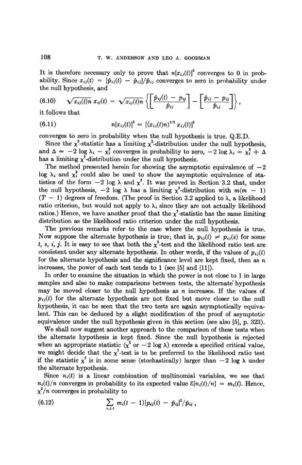
108 T. W. ANDERSON AND LEO A. GOODMAN

It is therefore necessary only to prove that n[xij(t)]3 converges to 0 in prob- ability. Since xij(t) = [ pjp(t)-pij]/j converges to zero in probability under the null hypothesis, and

(6 .10) X x,nx, t) n [ A]t p ]n

it follows that

(6.11) n[xij(t)]3 - [(xj,(t)n)/2 Xij(t)]2

converges to zero in probability when the null hypothesis is true. Q.E.D. Since the x2-statistic has a limiting x2-distribution under the null hypothesis,

and A = -2 log Xi - converges in probability to zero, -2 log Xi = X2 + A has a limiting x2-distribution under the null hypothesis.

The method presented herein for showing the asymptotic equivalence of -2 log Xi and x2 could also be used to show the asymptotic equivalence of sta- tistics of the form -2 log X and x2. It was proved in Section 3.2 that, under the null hypothesis, -2 log X has a limiting x2-distribution with m(m - 1) (T - 1) degrees of freedom. (The proof in Section 3.2 applied to X, a likelihood ratio criterion, but would not apply to Xi since they are not actually likelihood ratios.) Hence, we have another proof that the x2-statistic has the same limiting distribution as the likelihood ratio criterion under the null hypothesis.

The previous remarks refer to the case where the null hypothesis is true. Now suppose the alternate hypothesis is true; that is, p,j(t) pij(S) for some t, s, i, j. It is easy to see 'that both the x2-test and the likelihood ratio test are conslstent under any alternate hypothesis. In other words, if the values of pij(t) for the alternate hypothesis and the significance level are kept fixed, then as n increases, the power of each test tends to 1 (see [5] and [11]).

In order to examine the situation in which the power is not close to 1 in large samples and also to make comparisons between tests, the alternate hypothesis may be moved closer to the null hypothesis as n increases. If the values of pi(t) for the alternate hypothesis are not fixed but move closer to the null hypothesis, it can be seen that the two tests are again asymptotically equiva- lent. This can be deduced by a slight modification of the proof of asymptotic equivalence under the null hypothesis given in this section (see also [5], p. 323).

We shall now suggest another approach to the comparison of these tests when the alternate hypothesis is kept fixed. Since the null hypothesis is rejected when an appropriate statistic (x2 or -2 log; X) exceeds a specified critical value, we might decide that the X2-test is to be preferred to the likelihood ratio test if the statistic x2 is in some sense (stochastically) larger than -2 log X under the alternate hypothesis.

Since ni(t) is a linear combination of multinomial variables, we see that n,(t)/n converges in probability to its expected value 8[nu(t)/n] = mi(t). Hence, x /n converges in probability to

(6.12) : mi(t - 1)[puj(t) -Pt]2/ij i,j,t

MARKOV CHA INS 109

and (-2 log X)/n convrerges in probability to

(6.13) 2 E mi(t - l)pi,(t) log [pj,(t)/p7]P, i,j,t

where

(6.14) pij pij(t) mi(t -)/ E mi(t - 1) = p lim pi. t t noo

The difference between (6.12) and (6.13) is approximately

(6.15) Emi (t - 1)pipj(t)-

Under the alternate hypothesis, these two stochastic limits. differ from 0, and computation of them suggests which test is better. If (pij(t) - pj)/pij is small, then there will be only a small difference between the two limits. When the alternative is some composite hypothesis, as is usually the case when X2- tests are applied, then these stochastic limits can be computed and compared for the simple alternatives that are included in the alternate hypothesis.

This method for comparing tests is somewhat related to Cochran's comment (see p. 323 in [5]) that either (a) the significance probability can be made to decrease as n increases, thus reducing the chance of an error of type I, or (b) the alternate hypothesis can be moved steadily closer to the null hypothesis. Method (b) was discussed in [3]. If method (a) is used, then the critical value of the statistic (X2 or - log X) will increase as n increases. When the critical value has the form on, where c is a constant (there may be some question as to whether this form for the critical value is really suitable), we see from the remarks in the preceding paragraph that the power of a test will tend to 1 if c is less than the stochastic limit and it will tend to 0 if c is greater than the stochastic limit. Hence, by this approach we find that the power of the X2-test can be quite different from the power of the likelihood ratio test, and some approximate computations can suggest which test is to be preferred.

However, a more appealing approach is to vary the significance level so the ratio of significance level tG the probability of some particular Type II error approaches a limit (or at least it seems that desirable sequences of significance points lie between c' and cn). While the usual asymptotic theory does not give enough information to handle this problem, the comparison of stochastic limits may suggest a comparison of powers.

The methods of comparison discussed herein can also be used in the study of the x2 and likelihood ratio methods for ordinary contingency tables. We have seen that, in a certain sense, the x2 and likelihood ratio methods are not equiva- lent when the alternate hypothesis is true and fixed, and we have suggested a method for determining which test is to be preferred.

REFERENCES

[1] T. W. ANDERSON, "Probability models for analyzing time changes in attitudes," RAND Research Memorandum No. 455, 1951.

110 T. W. ANDERSON AND LEO A. GOODMAN

12] T. W. ANDERSON, "Probability models for analyzing time changes in attitudes," Mathematical Thinking in the Social Sciences, edited by Paul F. Lazarsfeld, The Free Press, Glencoe, Illinois, 1954.

[3] M. S. BARTLETT, "The frequency goodness of fit test for probability chains," Proc. Cambridge Philos. Soc., Vol. 47 (1951), pp. 86-95.

[4] H. CHERNOFF, "Large-sample theory: parametric case," Ann. Math. Stat. Vol. 27 (1956), pp. 1-22.

[5] W. G. COCHRAN,."The X2-test of goodness of fit," Ann. Math. Stat., Vol. 23 (1952), pp. 315-345.

[61 H. CRAMbR, Mathematical Methods of Statistics, Princeton University Press, Prince- ton, 1946.

[71 W. FELLER, An Introduction to Probability Theory and Its Applications, Vol. 1, John Wiley and Sons, New York, 1950.

[8] L. A. GARDNER, JR., "Some estimation and distribution problems in information theory," Master's Essay, Columbia University Library, 1954.

[91 L. A. GOODMAN, "On the statistical analysis of Markov chains" (abstract), Ann. Math. Stat., Vol. 26 (1955), p. 771.

[101 P. G. HOEL, "A test for Markoff chains," Biometrika, Vol. 41 (1954), pp. 430-433. [111 J. NEYMAN, "Contribution to the theory of the X2-test," Proceedings of the Berkeley

Symposium on Mathematical Statistics and Probability, University of California Press, Berkeley, 1949, pp. 239-274.