An intriguing failing of convolutional neural networksand the CoordConv solution

Rosanne Liu1 Joel Lehman1 Piero Molino1 Felipe Petroski Such1 Eric Frank1

Alex Sergeev2 Jason Yosinski1

1Uber AI Labs, San Francisco, CA, USA 2Uber Technologies, Seattle, WA, USA

{rosanne,joel.lehman,piero,felipe.such,mysterefrank,asergeev,yosinski}@uber.com

Abstract

Few ideas have enjoyed as large an impact on deep learning as convolution. For anyproblem involving pixels or spatial representations, common intuition holds thatconvolutional neural networks may be appropriate. In this paper we show a strikingcounterexample to this intuition via the seemingly trivial coordinate transformproblem, which simply requires learning a mapping between coordinates in (x, y)Cartesian space and coordinates in one-hot pixel space. Although convolutionalnetworks would seem appropriate for this task, we show that they fail spectacularly.We demonstrate and carefully analyze the failure first on a toy problem, at whichpoint a simple fix becomes obvious. We call this solution CoordConv, whichworks by giving convolution access to its own input coordinates through the use ofextra coordinate channels. Without sacrificing the computational and parametricefficiency of ordinary convolution, CoordConv allows networks to learn eithercomplete translation invariance or varying degrees of translation dependence, asrequired by the end task. CoordConv solves the coordinate transform problem withperfect generalization and 150 times faster with 10–100 times fewer parametersthan convolution. This stark contrast raises the question: to what extent has thisinability of convolution persisted insidiously inside other tasks, subtly hamperingperformance from within? A complete answer to this question will require furtherinvestigation, but we show preliminary evidence that swapping convolution forCoordConv can improve models on a diverse set of tasks. Using CoordConv ina GAN produced less mode collapse as the transform between high-level spatiallatents and pixels becomes easier to learn. A Faster R-CNN detection modeltrained on MNIST detection showed 24% better IOU when using CoordConv, andin the Reinforcement Learning (RL) domain agents playing Atari games benefitsignificantly from the use of CoordConv layers.

1 IntroductionConvolutional neural networks (CNNs) [17] have enjoyed immense success as a key tool for enablingeffective deep learning in a broad array of applications, like modeling natural images [36, 16], imagesof human faces [15], audio [33], and enabling agents to play games in domains with synthetic imagerylike Atari [21]. Although straightforward CNNs excel at many tasks, in many other cases progresshas been accelerated through the development of specialized layers that complement the abilitiesof CNNs. Detection models like Faster R-CNN [27] make use of layers to compute coordinatetransforms and focus attention, spatial transformer networks [13] make use of differentiable camerasto transform data from the output of one CNN into a form more amenable to processing with another,

32nd Conference on Neural Information Processing Systems (NeurIPS 2018), Montréal, Canada.

arX

iv:1

807.

0324

7v2

[cs

.CV

] 3

Dec

201

8

Figure 1: Toy tasks considered in this paper. The *conv block represents a network comprised ofone or more convolution, deconvolution (convolution transpose), or CoordConv layers. Experimentscompare networks with no CoordConv layers to those with one or more.

and some generative models like DRAW [8] iteratively perceive, focus, and refine a canvas ratherthan using a single pass through a CNN to generate an image. These models were all created byneural network designers that intuited some inability or misguided inductive bias of standard CNNsand then devised a workaround.

In this work, we expose and analyze a generic inability of CNNs to transform spatial representationsbetween two different types: from a dense Cartesian representation to a sparse, pixel-based represen-tation or in the opposite direction. Though such transformations would seem simple for networksto learn, it turns out to be more difficult than expected, at least when models are comprised of thecommonly used stacks of convolutional layers. While straightforward stacks of convolutional layersexcel at tasks like image classification, they are not quite the right model for coordinate transform.

The main contributions of this paper are as follows:

1. We define a simple toy dataset, Not-so-Clevr, which consists of squares randomly positionedon a canvas (Section 2).

2. We define the CoordConv operation, which allows convolutional filters to know where theyare in Cartesian space by adding extra, hard-coded input channels that contain coordinatesof the data seen by the convolutional filter. The operation may be implemented via a coupleextra lines of Tensorflow (Section 3).

3. Throughout the rest of the paper, we examine the coordinate transform problem startingwith the simplest scenario and ending with the most complex. Although results on toyproblems should generally be taken with a degree of skepticism, starting small allows us topinpoint the issue, exploring and understanding it in detail. Later sections then show thatthe phenomenon observed in the toy domain indeed appears in more real-world settings.We begin by showing that coordinate transforms are surprisingly difficult even when theproblem is small and supervised. In the Supervised Coordinate Classification task, given apixel’s (x, y) coordinates as input, we train a CNN to highlight it as output. The SupervisedCoordinate Regression task entails the inverse: given an input image containing a singlewhite pixel, output its coordinates. We show that both problems are harder than expectedusing convolutional layers but become trivial by using a CoordConv layer (Section 4).

4. The Supervised Rendering task adds complexity to the above by requiring a network to painta full image from the Not-so-Clevr dataset given the (x, y) coordinates of the center of asquare in the image. The task is still fully supervised, but as before, the task is difficult tolearn for convolution and trivial for CoordConv (Section 4.3).

5. We show that replacing convolutional layers with CoordConv improves performance in avariety of tasks. On two-object Sort-of-Clevr [29] images, Generative Adversarial Networks(GANs) and Variational Autoencoders (VAEs) using CoordConv exhibit less mode collapse,perhaps because ease of learning coordinate transforms translates to ease of using latentsto span a 2D Cartesian space. Larger GANs on bedroom scenes with CoordConv offergeometric translation that was never observed in regular GAN. Adding CoordConv to aFaster R-CNN produces much better object boxes and scores. Finally, agents learning to

2

Figure 2: The Not-so-Clevr dataset. (a) Example one-hot center images Pi from the dataset. (b) Thepixelwise sum of the entire train and test splits for uniform vs. quadrant splits. (c) and (d) Analagousdepictions of the canvas images Ii from the dataset. Best viewed electronically with zoom.

play Atari games obtain significantly higher scores on some but not all games, and theynever do significantly worse (Section 5).

6. To enable other researchers to reproduce experiments in this paper, and benefit from usingCoordConv as a simple drop-in replacement of the convolution layer in their models, werelease our code at https://github.com/uber-research/coordconv.

With reference to the above numbered contributions, the reader may be interested to know that thecourse of this research originally progressed in the 5→ 2 direction as we debugged why progressivelysimpler problems continued to elude straightforward modeling. But for ease of presentation, we giveresults in the 2→ 5 direction. A progression of the toy problems considered is shown in Figure 1.

2 Not-so-Clevr datasetWe define the Not-so-Clevr dataset and make use of it for the first experiments in this paper. Thedataset is a single-object, grayscale version of Sort-of-CLEVR [29], which itself is a simpler versionof the Clevr dataset of rendered 3D shapes [14]. Note that the series of Clevr datasets have beentypically used for studies regarding relations and visual question answering, but we here use themfor supervised learning and generative models. Not-so-Clevr consists of 9× 9 squares placed on a64 × 64 canvas. Square positions are restricted such that the entire square lies within the 64 × 64grid, so that square centers fall within a slightly smaller possible area of 56× 56. Enumerating thesepossible center positions results in a dataset with a total of 3,136 examples. For each example squarei, the dataset contains three fields:

• Ci ∈ R2, its center location in (x, y) Cartesian coordinates,• Pi ∈ R64×64, a one-hot representation of its center pixel, and• Ii ∈ R64×64, the resulting 64× 64 image of the square painted on the canvas.

We define two train/test splits of these 3,136 examples: uniform, where all possible center locationsare randomly split 80/20 into train vs. test sets, and quadrant, where three of four quadrants are in thetrain set and the fourth quadrant in the test set. Examples from the dataset and both splits are depictedin Figure 2. To emphasize the simplicity of the data, we note that this dataset may be generated inonly a line or two of Python using a single convolutional layer with filter size 9 × 9 to paint thesquares from a one-hot representation.1

3 The CoordConv layerThe proposed CoordConv layer is a simple extension to the standard convolutional layer. We assumefor the rest of the paper the case of two spatial dimensions, though operators in other dimensionsfollow trivially. Convolutional layers are used in a myriad of applications because they often workwell, perhaps due to some combination of three factors: they have relatively few learned parameters,they are fast to compute on modern GPUs, and they learn a function that is translation invariant (atranslated input produces a translated output).

1For example, ignoring import lines and train/test splits:onehots = np.pad(np.eye(3136).reshape((3136, 56, 56, 1)), ((0,0), (4,4), (4,4), (0,0)), "constant");images = tf.nn.conv2d(onehots, np.ones((9, 9, 1, 1)), [1]*4, "SAME")

3

Figure 3: Comparison of 2D convolutional and CoordConv layers. (left) A standard convolutionallayer maps from a representation block with shape h × w × c to a new representation of shapeh′ × w′ × c′. (right) A CoordConv layer has the same functional signature, but accomplishes themapping by first concatenating extra channels to the incoming representation. These channels containhard-coded coordinates, the most basic version of which is one channel for the i coordinate and onefor the j coordinate, as shown above. Other derived coordinates may be input as well, like the radiuscoordinate used in ImageNet experiments (Section 5).

The CoordConv layer keeps the first two of these properties—few parameters and efficientcomputation—but allows the network to learn to keep or to discard the third—translation invariance—as is needed for the task being learned. It may appear that doing away with translation invariancewill hamper networks’ abilities to learn generalizable functions. However, as we will see in latersections, allocating a small amount of network capacity to model non-translation invariant aspects ofa problem can enable far more trainable models that also generalize far better.

The CoordConv layer can be implemented as a simple extension of standard convolution in whichextra channels are instantiated and filled with (constant, untrained) coordinate information, afterwhich they are concatenated channel-wise to the input representation and a standard convolutionallayer is applied. Figure 3 depicts the operation where two coordinates, i and j, are added. Concretely,the i coordinate channel is an h×w rank-1 matrix with its first row filled with 0’s, its second row with1’s, its third with 2’s, etc. The j coordinate channel is similar, but with columns filled in with constantvalues instead of rows. In all experiments, we apply a final linear scaling of both i and j coordinatevalues to make them fall in the range [−1, 1]. For convolution over two dimensions, two (i, j)coordinates are sufficient to completely specify an input pixel, but if desired, further channels can beadded as well to bias models toward learning particular solutions. In some of the experiments thatfollow, we have also used a third channel for an r coordinate, where r =

√(i− h/2)2 + (j − w/2)2.

The full implementation of the CoordConv layer is provided in Section S9. Let’s consider next a fewproperties of this operation.

Number of parameters. Ignoring bias parameters (which are not changed), a standard convolu-tional layer with square kernel size k and with c input channels and c′ output channels will containcc′k2 weights, whereas the corresponding CoordConv layer will contain (c+ d)c′k2 weights, whered is the number of coordinate dimensions used (e.g. 2 or 3). The relative increase in parameters issmall to moderate, depending on the original number of input channels. 2

Translation invariance. CoordConv with weights connected to input coordinates set by initializa-tion or learning to zero will be translation invariant and thus mathematically equivalent to ordinaryconvolution. If weights are nonzero, the function will contain some degree of translation dependence,the precise form of which will ideally depend on the task being solved. Similar to locally connectedlayers with unshared weights, CoordConv allows learned translation dependence, but by contrast

2A CoordConv layer implemented via the channel concatenation discussed entails an increase of dc′k2

weights. However, if k > 1, not all k2 connections from coordinates to each output unit are necessary, asspatially neighboring coordinates do not provide new information. Thus, if one cares acutely about minimizingthe number of parameters and operations, a k × k conv may be applied to the input data and a 1× 1 conv to thecoordinates, then the results added. In this paper we have used the simpler, if marginally inefficient, channelconcatenation version that applies a single convolution to both input data and coordinates. However, almost allexperiments use 1× 1 filters with CoordConv.

4

it requires far fewer parameters: (c + d)c′k2 vs. hwcc′k2 for spatial input size h × w. Note thatall CoordConv weights, even those to coordinates, are shared across all positions, so translationdependence comes only from the specification of coordinates; one consequence is that, as withordinary convolution but unlike locally connected layers, the operation can be expanded outside theoriginal spatial domain if the appropriate coordinates are extrapolated.

Relations to other work. CoordConv layers are related to many other bodies of work. Composi-tional Pattern Producing Networks (CPPNs) [31] implement functions from coordinates in arbitrarilymany dimensions to one or more output values. For example, with two input dimensions and Noutput values, this can be thought of as painting N separate grayscale pictures. CoordConv can thenbe thought of as a conditional CPPN where output values depend not only on coordinates but alsoon incoming data. In one CPPN-derived work [11], researchers did train networks that take as inputboth coordinates and incoming data for their use case of synthesizing a drum track that could deriveboth from a time coordinate and from other instruments (input data) and trained using interactiveevolution. With respect to that work, we may see CoordConv as a simpler, single-layer mechanismthat fits well within the paradigm of training large networks with gradient descent on GPUs. In asimilar vein, research on convolutional sequence to sequence learning [7] has used fixed and learnedposition embeddings at the input layer; in that work, positions were represented via an overcompletebasis that is added to the incoming data rather than being compactly represented and input as separatechannels. In some cases using overcomplete sine and cosine bases or learned encodings for locationshas seemed to work well [34, 24]. Connections can also be made to mechanisms of spatial attention[13] and to generative models that separately learn what and where to draw [8, 26]. While such worksmight appear to provide alternative solutions to the problem explored in this paper, in reality, similarcoordinate transforms are often embedded within such models (e.g. a spatial transformer networkcontains a localization network that regresses from an image to a coordinate-based representation[13]) and might also benefit from CoordConv layers.

Moreover, several previous works have found it necessary or useful to inject geometric informationto networks, for example, in prior networks to enhance spatial smoothness [32], in segmentationnetworks [2, 20], and in robotics control through a spatial softmax layer and an expected coordinatelayer that map scenes to object locations [18, 5]. However, in those works it is often seen as aminor detail in a larger architecture which is tuned to a specific task and experimental project, anddiscussions of this necessity are scarce. In contrast, our research (a) examines this necessity in depthas its central thrust, (b) reduces the difficulty to its minimal form (coordinate transform), leadingto a simple single explanation that unifies previously disconnected observations, and (c) presentsone solution used in various forms by others as a unified layer, easily included anywhere in anyconvolutional net. Indeed, the wide range of prior works provide strong evidence of the generality ofthe core coordinate transform problem across domains, suggesting the significant value of a workthat systematically explores its impact and collects together these disparate previous references.

Finally, we note that challenges in learning coordinate transformations are not unknown in machinelearning, as learning a Cartesian-to-polar coordinate transform forms the basis of the classic two-spirals classification problem [4].

4 Supervised Coordinate tasks4.1 Supervised Coordinate ClassificationThe first and simplest task we consider is Supervised Coordinate Classification. Illustrated at the topof Figure 1, given an (x, y) coordinate as input, a network must learn to paint the correct output pixel.This is simply a multi-class classification problem where each pixel is a class. Why should we studysuch a toy problem? If we expect to train generative models that can transform high level latents likehorizontal and vertical position into pixel data, solving this toy task would seem a simple prerequisite.We later verify that performance on this task does in fact predict performance on larger problems.

In Figure 4 we depict training vs. test accuracy on the task for both uniform and quadrant train/testsplits. For convolutional models3(6 layers of deconvolution with stride 2, see Section S1 in theSupplementary Information for architecture details) on uniform splits, we find models that generalizesomewhat, but 100% test accuracy is never achieved, with the best model achieving only 86% test

3For classification, convolutions and CoordConvs are actually deconvolutional on certain layers whenresolutions must be expanded, but we refer to the models as conv or CoordConv for simplicity.

5

Convolution

CoordConvPerfect test accuracy takes 10–20 seconds

Convergence to 80% test accuracy takes 4000 seconds

Figure 4: Performance of convolution and CoordConv on Supervised Coordinate Classification.(left column) Final test vs. train accuracy. On the easier uniform split, convolution never attainsperfect test accuracy, though the largest models memorize the training set. On the quadrant split,generalization is almost zero. CoordConv attains perfect train and test accuracy on both splits. Oneof the main results of this paper is that the translation invariance in ordinary convolution does notlead to coordinate transform generalization even to neighboring pixels! (right column) Test accuracyvs. training time of the best uniform-split models from the left plot (any reaching final test accuracy≥ 0.8). The convolution models never achieve more than about 86% accuracy, and training is slow:the fastest learning models still take over an hour to converge. CoordConv models learn severalhundred times faster, attaining perfect accuracy in seconds.

accuracy. This is surprising: because of the way the uniform train/test splits were created, all testpixels are close to multiple train pixels. Thus, we reach a first striking conclusion: learning a smoothfunction from (x, y) to one-hot pixel is difficult for convolutional networks, even when trained withsupervision, and even when supervision is provided on all sides. Further, training a convolutionalmodel to 86% accuracy takes over an hour and requires about 200k parameters (see Section S2 in theSupplementary Information for details on training). On the quadrant split, convolutional models areunable to generalize at all. Figure 5 shows sums over training set and test set predictions, showingvisually both the memorization of the convolutional model and its lack of generalization.

In striking contrast, CoordConv models attain perfect performance on both data splits and do so withonly 7.5k parameters and in only 10–20 seconds. The parsimony of parameters further confirms theyare simply more appropriate models for the task of coordinate transform [28, 10, 19].

4.2 Supervised Coordinate RegressionBecause of the surprising difficulty of learning to transform coordinates from Cartesian to a pixel-based, we examine whether the inverse transformation from pixel-based to Cartesian is equallydifficult. This is the type of transform that could be employed by a VAE encoder or GAN discriminatorto transform pixel information into higher level latents encoding locations of objects in a scene.

We experimented with various convolutional network structures, and found a 4-layer convolutionalnetwork with fully connected layers (85k parameters, see Section S3 for details) can fit the uniformtraining split and generalize well (less than half a pixel error on average), but that same architecturecompletely fails on the quadrant split. A smaller fully-convolutional architecture (12k parameters, seeSection S3) can be tuned to achieve limited generalization on the quadrant split (around five pixelserror on average) as shown in Figure 5 (right column), but it performs poorly on the uniform split.

A number of factors may have led to the observed variation of performance, including the use ofmax-pooling, batch normalization, and fully-connected layers. We have not fully and separatelymeasured how much each factor contributes to poor performance on these tasks; rather we reportonly that our efforts to find a workable architecture across both splits did not yield any winners. Incontrast, a 900 parameter CoordConv model, where a single CoordConv layer is followed by severallayers of standard convolution, trains quickly and generalizes in both the uniform and quadrant splits.See Section S3 in Supplementary Information for more details. These results suggest that the inversetransformation requires similar considerations to solve as the Cartesian-to-pixel transformation.

6

Convolution prediction

CoordConv prediction

Ground truth

Supervised Coordinate Classification Supervised Coordinate RegressionTrain Test Train Test

Figure 5: Comparison of convolutional and CoordConv models on the Supervised CoordinateClassification and Regression tasks, on a quadrant split. (left column) Results on the seeminglysimple classification task where the network must highlight one pixel given its (x, y) coordinates asinput. Images depict ground truth or predicted probabilities summed across the entire train or test setand then normalized to make use of the entire black to white image range. Thus, e.g., the top-leftimage shows the sum of all train set examples. The conv predictions on the train set cover it well,although the amount of noise in predictions hints at the difficulty with which this model eventuallyattained 99.6% train accuracy by memorization. The conv predictions on the test set are almostentirely incorrect, with two pixel locations capturing the bulk of the probability for all locations inthe test set. By contrast, the CoordConv model attains 100% accuracy on both the train and testsets. Models used: conv–6 layers of deconv with strides 2; CoordConv–5 layers of 1×1 conv, firstlayer is CoordConv. Details in Section S2. (right column) The regression task poses the inverseproblem: predict real-valued (x, y) coordinates from a one-hot pixel input. As before, the convmodel memorizes poorly and largely fails to generalize, while the CoordConv model fits train andtest set perfectly. Thus we observe the coordinate transform problem to be difficult in both directions.Models used: conv–9-layer fully-convolution with global pooling; CoordConv–5 layers of conv withglobal pooling, first layer is CoordConv. Details in Section S3.

4.3 Supervised Rendering

Moving beyond the domain of single pixel coordinate transforms, we compare performance ofconvolutional vs. CoordConv networks on the Supervised Rendering task, which requires a networkto produce a 64× 64 image with a square painted centered at the given (x, y) location. As shown inFigure 6, we observe the same stark contrast between convolution and CoordConv. Architecturesused for both models can be seen in Section S1 in the Supplementary Information, along with furtherplots, details of training, and hyperparameter sweeps given in Section S4.

5 Applicability to Image Classification, Object Detection, GenerativeModeling, and Reinforcement Learning

Given the starkly contrasting results above, it is natural to ask how much the demonstrated inabilityof convolution at coordinate transforms infects other tasks. Does the coordinate transform hurdlepersist insidiously inside other tasks, subtly hampering performance from within? Or do networksskirt the issue by learning around it, perhaps by representing space differently, e.g. via non-Cartesianrepresentations like grid cells [1, 6, 3]? A complete answer to this question is beyond the scope of thispaper, but encouraging preliminary evidence shows that swapping Conv for CoordConv can improvea diverse set of models — including ResNet-50, Faster R-CNN, GANs, VAEs, and RL models.

7

0.0 0.2 0.4 0.6 0.8 1.0Train IOU

0.0

0.2

0.4

0.6

0.8

1.0

Test

IOU

Deconv uniformDeconv quadrantCoordConv uniformCoordConv quadrant

Figure 6: Results on the Supervised Rendering task. As with the Supervised Coordinate Classificationand Regression tasks, we see the same vast separation in training time and generalization betweenconvolution models and CoordConv models. (left) Test intersection over union (IOU) vs TrainIOU. We show all attempted models on the uniform and quadrant splits, including some CoordConvmodels whose hyperparameter selections led to worse than perfect performance. (right) Test IOUvs. training time of the best uniform-split models from the left plot (any reaching final test IOU≥ 0.8). Convolution models never achieve more than about IOU 0.83, and training is slow: the fastestlearning models still take over two hours to converge vs. about a minute for CoordConv models.

ImageNet Classification As might be expected for tasks requiring straightforward translationinvariance, CoordConv does not help significantly when tested with image classification. Adding asingle extra 1×1 CoordConv layer with 8 output channels improves ResNet-50 [9] Top-5 accuracy bya meager 0.04% averaged over five runs for each treatment; however, this difference is not statisticallysignificant. It is at least reassuring that CoordConv doesn’t hurt the performance since it can alwayslearn to ignore coordinates. This result was obtained using distributed training on 100 GPUs withHorovod [30]; see Section S5 in Supplementary Information for more details.

Object Detection In object detection, models look at pixel space and output bounding boxes inCartesian space. This creates a natural coordinate transform problem which makes CoordConvseemingly a natural fit. On a simple problem of detecting MNIST digits scattered on a canvas, wefound the test intersection-over-union (IOU) of a Faster R-CNN network improved by 24% whenusing CoordConv. See Section S6 in Supplementary Information for details.

Generative Modeling Well-trained generative models can generate visually compelling images[23, 15, 36], but careful inspection can reveal mode collapse: images are of an attractive quality, butsample diversity is far less than diversity present in the dataset. Mode collapse can occur in manydimensions, including those having to do with content, style, or position of components of a scene.We hypothesize that mode collapse of position may be due to the difficulty of learning straightforwardtransforms from a high-level latent space containing coordinate information to pixel space and thatusing CoordConv could help. First we investigate a simple task of generating colored shapes with,in particular, all possible geometric locations, using both GANs and VAEs. Then we scale up theproblem to Large-scale Scene Understanding (LSUN) [35] bedroom scenes with DCGAN [25],through distributed training using Horovod [30].

Using GANs to generate simple colored objects, Figure 7a-d show sampled images and modelcollapse analyses. We observe that a convolutional GAN exhibits collapse of a two-dimensionaldistribution to a one-dimensional manifold. The corresponding CoordConv GAN model generatesobjects that better cover the 2D Cartesian space while using 7% of the parameters of the conv GAN.Details of the dataset and training can be seen in Section S7.1 in the Supplementary Information. Asimilar story with VAEs is discussed in Section S7.2.

With LSUN, samples are shown in Figure 7e, and more in Section S7.3 in the SupplementaryInformation. We observe (1) qualitatively comparable samples when drawing randomly from eachmodel, and (2) geometric translating behavior during latent space interpolation.

Latent space interpolation4 demonstrates that in generating colored objects, motions through latentspace generate coordinated object motion. In LSUN, while with convolution we see frozen objectsfading in and out, with CoordConv, we instead see smooth geometric transformations includingtranslation and deformation.

4https://www.youtube.com/watch?v=YefMbLqS7Jg

8

Figure 7: Real images and generated images by GAN and CoordConv GAN. Both models learn thebasic concepts similarly well: two objects per image, one red and one blue, their size is fixed, andtheir positions can be random (a). However, plotting the spread of object centers over 1000 samples,we see that CoordConv GAN samples cover the space significantly better (average entropy: Data red4.0, blue 4.0, diff 3.5; GAN red 3.13, blue 2.69, diff 2.81; CoordConv GAN red 3.30, blue 2.93, diff2.62), while GAN samples exhibit mode collapse on where objects can be (b). In terms of relativelocations between the two objects, both model exhibit a certain level of model collapse, CoordConvis worse (c). The averaged image of CoordConv GAN is smoother and closer to that of data (d). WithLSUN, sampled images are shown (e). All models used in generation are the best out of many runs.

Figure 8: Results using A2C to train on Atari games. Out of 9 games, (a) in 6 CoordConv improvesover convolution, (b) in 2 performs similarly, and (c) on 1 it is slightly worse.

Reinforcement Learning Adding a CoordConv layer to an actor network within A2C [22] pro-duces significant improvements on some games, but not all, as shown in Figure 8. We also triedadding CoordConv to our own implementation of Distributed Prioritized Experience Replay (Ape-X)[12], but we did not notice any immediate difference. Details of training are included in Section S8.

6 Conclusions and Future WorkWe have shown the curious inability of CNNs to model the coordinate transform task, shown a simplefix in the form of the CoordConv layer, and given results that suggest including these layers canboost performance in a wide range of applications. Future work will further evaluate the benefits ofCoordConv in large-scale datasets, exploring its ability against perturbations of translation, its impactin relational reasoning [29], language tasks, video prediction, with spatial transformer networks [13],and with cutting-edge generative models [8].

9

Acknowledgements

The authors gratefully acknowledge Zoubin Ghahramani, Peter Dayan, and Ken Stanley for insightfuldiscussions. We are also grateful to the entire Opus team and Machine Learning Platform team insideUber for providing our computing platform and for technical support.

References[1] Andrea Banino, Caswell Barry, Benigno Uria, Charles Blundell, Timothy Lillicrap, Piotr

Mirowski, Alexander Pritzel, Martin J Chadwick, Thomas Degris, Joseph Modayil, et al.Vector-based navigation using grid-like representations in artificial agents. Nature, page 1,2018.

[2] Clemens-Alexander Brust, Sven Sickert, Marcel Simon, Erik Rodner, and Joachim Denzler.Convolutional patch networks with spatial prior for road detection and urban scene under-standing. In International Conference on Computer Vision Theory and Applications (VISAPP),2015.

[3] C. J. Cueva and X.-X. Wei. Emergence of grid-like representations by training recurrent neuralnetworks to perform spatial localization. ArXiv e-prints, March 2018.

[4] Scott E Fahlman and Christian Lebiere. The cascade-correlation learning architecture. InAdvances in neural information processing systems, pages 524–532, 1990.

[5] Chelsea Finn, Xin Yu Tan, Yan Duan, Trevor Darrell, Sergey Levine, and Pieter Abbeel. Deepspatial autoencoders for visuomotor learning. In 2016 IEEE International Conference onRobotics and Automation (ICRA), pages 512–519. IEEE, 2016.

[6] Mathias Franzius, Henning Sprekeler, and Laurenz Wiskott. Slowness and sparseness lead toplace, head-direction, and spatial-view cells. PLoS computational biology, 3(8):e166, 2007.

[7] Jonas Gehring, Michael Auli, David Grangier, Denis Yarats, and Yann N. Dauphin. Convolu-tional sequence to sequence learning. CoRR, abs/1705.03122, 2017.

[8] Karol Gregor, Ivo Danihelka, Alex Graves, Danilo Jimenez Rezende, and Daan Wierstra. Draw:A recurrent neural network for image generation. arXiv preprint arXiv:1502.04623, 2015.

[9] Kaiming He, Xiangyu Zhang, Shaoqing Ren, and Jian Sun. Deep residual learning for imagerecognition. CoRR, abs/1512.03385, 2015.

[10] Geoffrey E Hinton and Drew Van Camp. Keeping neural networks simple by minimizingthe description length of the weights. In Proceedings of the sixth annual conference onComputational learning theory, pages 5–13. ACM, 1993.

[11] Amy K Hoover and Kenneth O Stanley. Exploiting functional relationships in musical composi-tion. Connection Science, 21(2-3):227–251, 2009.

[12] Dan Horgan, John Quan, David Budden, Gabriel Barth-Maron, Matteo Hessel, HadoVan Hasselt, and David Silver. Distributed prioritized experience replay. arXiv preprintarXiv:1803.00933, 2018.

[13] Max Jaderberg, Karen Simonyan, Andrew Zisserman, et al. Spatial transformer networks. InAdvances in neural information processing systems, pages 2017–2025, 2015.

[14] Justin Johnson, Bharath Hariharan, Laurens van der Maaten, Li Fei-Fei, C Lawrence Zitnick,and Ross Girshick. Clevr: A diagnostic dataset for compositional language and elementaryvisual reasoning. In Computer Vision and Pattern Recognition (CVPR), 2017 IEEE Conferenceon, pages 1988–1997. IEEE, 2017.

[15] Tero Karras, Timo Aila, Samuli Laine, and Jaakko Lehtinen. Progressive growing of gans forimproved quality, stability, and variation. In ICLR, volume abs/1710.10196, 2018.

10

[16] Alex Krizhevsky, Ilya Sutskever, and Geoff Hinton. Imagenet classification with deep convo-lutional neural networks. In Advances in Neural Information Processing Systems 25, pages1106–1114, 2012.

[17] Yann LeCun, Yoshua Bengio, et al. Convolutional networks for images, speech, and time series.The handbook of brain theory and neural networks, 3361(10):1995, 1995.

[18] Sergey Levine, Chelsea Finn, Trevor Darrell, and Pieter Abbeel. End-to-end training of deepvisuomotor policies. The Journal of Machine Learning Research, 17(1):1334–1373, 2016.

[19] Chunyuan Li, Heerad Farkhoor, Rosanne Liu, and Jason Yosinski. Measuring the IntrinsicDimension of Objective Landscapes. In International Conference on Learning Representations,April 2018.

[20] Yecheng Lyu and Xinming Huang. Road segmentation using cnn with gru. arXiv preprintarXiv:1804.05164, 2018.

[21] V. Mnih, K. Kavukcuoglu, D. Silver, A. Graves, I. Antonoglou, D. Wierstra, and M. Riedmiller.Playing Atari with Deep Reinforcement Learning. ArXiv e-prints, December 2013.

[22] Volodymyr Mnih, Adria Puigdomenech Badia, Mehdi Mirza, Alex Graves, Timothy Lillicrap,Tim Harley, David Silver, and Koray Kavukcuoglu. Asynchronous methods for deep rein-forcement learning. In International Conference on Machine Learning, pages 1928–1937,2016.

[23] A. Nguyen, J. Yosinski, Y. Bengio, A. Dosovitskiy, and J. Clune. Plug & Play Generative Net-works: Conditional Iterative Generation of Images in Latent Space. ArXiv e-prints, November2016.

[24] Niki Parmar, Ashish Vaswani, Jakob Uszkoreit, Łukasz Kaiser, Noam Shazeer, and AlexanderKu. Image transformer. arXiv preprint arXiv:1802.05751, 2018.

[25] Alec Radford, Luke Metz, and Soumith Chintala. Unsupervised representation learning withdeep convolutional generative adversarial networks. arXiv preprint arXiv:1511.06434, 2015.

[26] Scott E Reed, Zeynep Akata, Santosh Mohan, Samuel Tenka, Bernt Schiele, and Honglak Lee.Learning what and where to draw. In Advances in Neural Information Processing Systems,pages 217–225, 2016.

[27] Shaoqing Ren, Kaiming He, Ross Girshick, and Jian Sun. Faster r-cnn: Towards real-timeobject detection with region proposal networks. In Advances in neural information processingsystems, pages 91–99, 2015.

[28] Jorma Rissanen. Modeling by shortest data description. Automatica, 14(5):465–471, 1978.

[29] Adam Santoro, David Raposo, David G Barrett, Mateusz Malinowski, Razvan Pascanu, PeterBattaglia, and Tim Lillicrap. A simple neural network module for relational reasoning. InAdvances in neural information processing systems, pages 4974–4983, 2017.

[30] A. Sergeev and M. Del Balso. Horovod: fast and easy distributed deep learning in TensorFlow.ArXiv e-prints, February 2018.

[31] Kenneth O Stanley. Compositional pattern producing networks: A novel abstraction of develop-ment. Genetic programming and evolvable machines, 8(2):131–162, 2007.

[32] Dmitry Ulyanov, Andrea Vedaldi, and Victor Lempitsky. Deep image prior. arXiv preprintarXiv:1711.10925, 2017.

[33] Aaron Van Den Oord, Sander Dieleman, Heiga Zen, Karen Simonyan, Oriol Vinyals, AlexGraves, Nal Kalchbrenner, Andrew Senior, and Koray Kavukcuoglu. Wavenet: A generativemodel for raw audio. arXiv preprint arXiv:1609.03499, 2016.

[34] Ashish Vaswani, Noam Shazeer, Niki Parmar, Jakob Uszkoreit, Llion Jones, Aidan N Gomez,Łukasz Kaiser, and Illia Polosukhin. Attention is all you need. In Advances in Neural Informa-tion Processing Systems, pages 6000–6010, 2017.

11

[35] Fisher Yu, Ari Seff, Yinda Zhang, Shuran Song, Thomas Funkhouser, and Jianxiong Xiao. Lsun:Construction of a large-scale image dataset using deep learning with humans in the loop. arXivpreprint arXiv:1506.03365, 2015.

[36] Han Zhang, Tao Xu, Hongsheng Li, Shaoting Zhang, Xiaolei Huang, Xiaogang Wang, andDimitris Metaxas. Stackgan: Text to photo-realistic image synthesis with stacked generativeadversarial networks. In IEEE Int. Conf. Comput. Vision (ICCV), pages 5907–5915, 2017.

12

Supplementary Information for:An intriguing failing of convolutional neural networks

and the CoordConv solution

S1 Architectures used for supervised painting tasks

Figure S1 depicts architectures used in each of the two supervised tasks going from coordinates toimages: Supervised Coordinate Classification (Section 4.1), and Supervised Rendering (Section 4.3).

In the case of convolution, or, in this case, transposed convolution (deconvolution), the same archi-tecture is used for both tasks, as shown in the top row of Figure S1, but we generally found theSupervised Rendering tasks requires wider layers (more channels). Top performing deconvolutionalmodels in Supervised Coordinate Classification have c = 1 or 2, while in Supervised Rendering weusually need c = 2, 3. In terms of convolutional filter size, filter sizes of 2 and 4 seem to outperform3 in Coordinate Classification, while in Rendering the difference is less distinctive.

Note that the CoordConv model only replaces the first layer with CoordConv (shown in green inFigure S1 ).

Figure S1: Deconvolutional and CoordConv architectures used in each of the two supervised tasks.“fs" stands for filter size, and “c" for channel size. We use a grid search on different ranges of themas displayed underneath each model, while allowing deconvolutional models a wider range in both.Green indicates a CoordConv layer.

13

5×103

1×104

2×104

5×104

105

2×105

5×105

106

2×106

Model size

0.0

0.2

0.4

0.6

0.8

1.0

Test

acc

urac

y

Deconv uniformDeconv quadrantCoordConv uniformCoordConv quadrant

Figure S2: Model size vs. test accuracy for the Supervised Coordinate Classification subtask onthe uniform split and quadrant split. Deconv models (blue) of many sizes achieve 80% or a littlehigher — but never perfect — test accuracy on the uniform split. On the quadrant split, while manymodels perform slightly better than chance (1/4096 = .000244) no model generalizes significantly.CoordConv model achieves perfect accuracy on both splits.

Because of the usage of different filter sizes and channel sizes, we end up training models with arange of sizes. Each is combined with further grid searches on hyperparameters including the learningrate, weight decay, and minibatch sizes. Therefore at the same size we end up with multiple modelswith a spread of performances, as shown in Figure S2 for the Supervised Coordinate Classificationtask. We repeat the same exact setting of experiments on both uniform and quadrant splits, whichresult in the same number of experiments. It is not obviously shown in Figure S2 because quadranttrainings are mostly poorly (at the bottom of the figure).

As can be seen, it seems unlikely that even larger models would perform better. They all basicallystruggle to get to a good test accuracy. This (1) confirms that performance is not simply beinglimited by model size, as well as (2) shows that working CoordConv models are one to two orders ofmagnitude smaller (7553 as opposed to 50k-1.6M parameters) than the best convolutional models.The model size vs. test performance plot on Supervised Rendering is similar (not shown), exceptCoordConv model in that case has a slightly larger number of parameters: 9490. CoordConv achievesperfect test IOU there while deconvolutional models struggle at sizes 183k to 1.6M.

S2 Further Supervised Coordinate Classification details

For deconvolutional models, we use the model structure as depicted in the top row in Figure S1, whilevarying the choice of filter size ({2, 3, 4}) and channel size multipliers ({1,2,3}), and each combinedwith a hyperparameter sweep of learning rate {0.001, 0.002, 0.005, 0.01, 0.02, 0.05}, and weightdecay {0.001, 0.01}. Models are trained using a softmax output with cross entropy loss with Adamoptimizer. We train 1000 epochs with minibatch size of 16 and 32. The learning rate is dropped to10% every 200 epochs for four times.

For CoordConv models, because it converges so fast and easy, we did not have to try a lot of settings— only 3 learning rates {0.01 0.001, 0.005} and they all learned perfectly well. There’s also no needfor learning rate schedules as it quickly converges in 10 seconds.

Figure S3 demonstrates how accurate and smooth the learned probability mass is with CoordConv,and not so much with Deconv. We first show the overall 64 × 64 map of logits, one for a trainingexample and one for a test example just right next to the train. Then we zoom in to a smallerregion to examine the intricacies. We can see that convolution, even though designed to act in atranslation-invariant way, shows artifacts of not being able to accomplish so.

14

Figure S3: Comparison of behaviors between Deconv model and CoordConv model on the SupervisedCoordinate Classification task. We select five horizontally neighboring pixels, containing samples inboth train and test splits, and zoom in on a 5× 9 section of the 64× 64 canvas so the detail of thelogits and predicted probabilities may be seen. The full 64× 64 map of logits of the first two samples(first in train, second in test) are also shown. The deconvolutional model outputs probabilities in adecidedly non-translation-invariant manner.

S3 Further Supervised Coordinate Regression details

Exact architectures applied in the Supervised Coordinate Regression task are described in tableS1. For the uniform split, the best-generalizing convolution architecture consisted of a stack ofalternating convolution and max-pooling layers, followed by a fully-connected layer and an outputlayer. This architecture was fairly robust to changes in hyperparameters. In contrast, for the quandrantsplit, the best-generalizing network consisted of strided convolutions feeding into a global-poolingoutput layer, and good performance was delicate. In particular, training and generalization wassensitive to the number of batch normalization layers (2), weight decay strength (5e-4), and optimizer(Adam, learning rate 5e-4). A single CoordConv architecture generalized perfectly with the samehyperparameters over both splits, and consisted of a single CoordConv layer followed by additionallayers of convolution, feeding into a global pooling output layer.

Table S1: Model Architectures for Supervised Coordinate Regression. FC: Fully-connected, MP:Max Pooling, GP: Global Pooling, BN: Batch normalization, s2: stride 2.

Conv CoordConv

UniformSplit

3×3, 16 - MP 2×2 - 3×3, 16 - MP 2×2 - 3×3,16 - MP 2×2 - 3×3, 16 - FC 64 - FC 2 1×1, 8 - 1×1, 8 - 1×1, 8 - 3×3,

8 - 3×3, 2 - GPQuadrantSplit

5×5 (s2), 16 - 1×1, 16 - BN - 3×3, 16 - 3×3(s2), 16 - 3×3 (s2), 16 - BN - 3×3 (s2), 16 -1×1, 16 - 3×3 (s2), 16 - 3×3, 2 - GP

S4 Further Supervised Rendering details

Both the architectural and experimental settings are similar to Section S2 except the loss used ispixelwise sigmoid output with cross entropy loss. We also tried mean squared error loss but theperformance is even weaker. We performed heavy hyperparameter sweeping and deliberate learningrate annealing for Deconv models (same as said in Section S2), while in CoordConv models it is fairlyeasy to find a good setting. All models trained with learning rates {0.001, 0.005}, weight decay {0,0.001}, filter size {1, 2} turned out to perform well after 1–2 minutes of training. Take the best model

15

obtained, Figure S4 and Figure S5 show the learned logits and pixelwise probability distributions forthree samples each, in the uniform and quadrant cases, respectively. We can see that the CoordConvmodel learns a much smoother and precise distribution. All samples are test samples.

Figure S4: Output comparison between Deconv and CoordConv models on three test samples. Modelsare trained on a uniform split. Logits are model’s direct output; pixelwise probability (pw-prob)is logits after Sigmoid. Conv outputs (middle columns) manage to get roughly right. CoordConvoutputs (right columns) are precisely correct and its logit maps are smooth.

Figure S5: Output comparison between Deconv and CoordConv models on three test samples. Modelsare trained on a quadrant split. Logits are model’s direct output; pixelwise probability (pw-prob)is logits after Sigmoid. Conv outputs (middle columns) failed mostly. Even with such a difficultgeneralization problem, CoordConv outputs (right columns) are precisely correct and its logit mapsare smooth.

S5 Further ImageNet classification details

We evaluate the potential of CoordConv in image classification with ImageNet experiments. We takeResNet-50 and run the baseline on distributed framework using 100 GPUs, with the open-sourceframework Horovod. For CoordConv variants, we add an extra CoordConv layer only in the beginning,which takes a 6-channel tensor containing image RBG, i, j coordinates and pixel distance to center r,and output 8 channels with 1×1 convolution. The increase of parameters is negligible. It then goes inwith the rest of ResNet-50.

Each model is run 5 times on the same setting to account for experimental variances. Table. S2 liststhe test result from each run in the end of 90 epochs. CoordConv model obtains better average resulton two of the three measures, however a one-sided t-test tells that the improvement on Top 5 accuracyis not quite statistically significant with p = .11.

16

Of all vision tasks, we might expect image classification to show the least performance change whenusing CoordConv instead of convolution, as classification is more about what is in the image thanwhere it is. This tiny amount of improvement validates that.

Table S2: ImageNet classification result comparison between a baseline ResNet-50 and CoordConvResNet-50. For each model three experiments are run, listed in three separate rows below.

Test loss Top-1 Accuracy Top-5 Accuracy

BaselineResNet-50

1.43005 0.75722 0.92622

1.42385 0.75844 0.9272

1.42634 0.75782 0.92754

1.42166 0.75692 0.92756

1.42671 0.75724 0.92708

Average 1.425722 0.757528 0.92712

CoordConvResNet-50

1.42335 0.75732 0.92802

1.42492 0.75836 0.92754

1.42478 0.75774 0.92818

1.42882 0.75702 0.92694

1.42438 0.75668 0.92714

Average 1.42525 0.757424 0.927564

S6 Further object detection details

The object detection experiments are on a dataset containing randomly rescaled and placed MNISTdigits on a 64× 64 canvas. To make it more akin to natural images, we generate a much larger canvasand then center crop it to be 64× 64, so that digits can be partially outside of the canvas. We keptimages that contain 5 digit objects whose centers are within the canvas. In the end we use 9000images as the training set and 1000 as test.

A schematic of the model architecture is illustrated in Figure S6. We use number of anchors A = 9,with sizes (15, 15), (20, 20), (25, 25), (15, 20), (20, 25), (20, 15), (25, 20), (15, 25), (25, 15). Inbox sampling (training mode), p_size and n_size are 6. In box non-maximum suppression (NMS)(test mode), the IOU threshold is 0.8 and maximum number of proposal boxes is 10. After the boxesare proposed and shifted, we do not have a downstream classification task, but just calculate the lossfrom the boxes. The training loss include box loss and score loss. As evaluation metric we alsocalculate IOUs between proposed boxes and ground truth boxes. Table. S3 lists those metrics obtainedthe test dataset, by both Conv and CoordConv models. We found that every metric is improved byCoordConv, and the average test IOU improved by about 24 percent.

17

Figure S6: Faster R-CNN architecture used for object detection on scattered MNIST digits. Greenindicates where coordinates are added. Note that the input image is used for demonstration purpose.The real dataset contains 5 digits on a canvas and allows overlapping. (Left) train mode with boxsampler. (Right) test mode with box NMS.

Table S3: MNIST digits detection result comparison between a Faster R-CNN model with regularconvolution vs. with CoordConv. Metrics are all on test set. Train IOU: average IOU betweensampled positive boxes (train mode) and ground truth; Test IOU-average): average IOU between 10selected boxes (test mode) and ground truth; Test IOU-select: average IOU between the best scoredbox and its closest ground truth.

Conv CoordConv % Improvement

Box loss 0.1003 0.0854 17.44

Score loss 0.5270 0.2526 108.63

Total loss (sum of the two above) 0.6271 0.3383 85.37

Train IOU 0.6388 0.6612 3.38

Test IOU-average 0.1508 0.1868 23.87

Test IOU-select 0.4965 0.6359 28.08

S7 Further generative modeling details

S7.1 GANs on colored shapes

Data. The dataset used to train the generative models is 50k red-and-blue-object images of size64× 64. We follow the same mechanism as Sort-of-Clevr, in that objects appear at random positionson a white background without overlapping, only limiting the number of objects to be 2 per image.The objects are always one red and one blue, of a randomly chosen shape out of {circle, square}.Examples of images from this dataset can be seen in the top row, leftmost column in Figure 7, at theintersection of “Real images" and “Random samples".

Architecture and training details. The z dimension to both regular GAN and CoordConv GANis 256. In GAN, the generator uses 4 layers of deconvolution with strides of 2 to project z to a64 × 64 image shape. The parameter size of the generator is 6,413,315. In CoordConv GAN, weadd coordinate channels only at the beginning, making the first layer CoordConv, and then continuewith normal Conv.. The generator in this case uses mostly (1,1) convolutions and has only 444,931parameters. The same discriminator is used for both models. In the case where we also turn the

18

discriminator to be CoordConv like, its first Conv layer is replaced by CoordConv, and the parametersize increases from 4,316,545 to 4,319,745. The details of both architectures can be seen in Table. S4.We trained two CoordConv GAN versions where CoordConv applies: 1) only in generator, and 2)in both generator and discriminator. They end up performing similarly well. The demonstratedexamples in all figures are from one in the latter case.

The change needed to make a generator whose first layer is fully-connected CoordConv is trivial.Instead of taking image tensors which already have Cartesian dimensions, the CoordConv generatorfirst tiles z vector into a full 64× 64 space, and then concatenate it with coordinates in that space.

To train each model we use a fixed learning rate 0.0001 for the discriminator and 0.0005 for thegenerator. In each iteration discriminator is trained once followed by generator trained twice. Therandom noise vector z is drawn from a uniform distribution between [−1, 1]. We train each modelfor 50 epochs and save the model in the end of every epoch. We repeat the training with the samehyperparameters 5 to 10 times for each, and pick the best model for each to show a fair comparisonin all figures.

Table S4: Model Architectures for GAN and CoordConv GAN used in the colored shape generation.In the case of CoordConv GAN, only the first layer is changed from regular Conv to CoordConv. FC:fully connected layer; s2: stride 2.

Generator Discriminator

GAN FC 8192 (reshape 4×4×512) - 5×5, 256 (s2)- 5×5, 128 (s2) - 5×5, 64 (s2) - 5×5, 3 (s2) -Tanh

5×5, 64 (s2) - 5×5, 128 (s2)- 5×5, 256 (s2) - 5×5, 512(s2) - 1CoordConv

GAN1×1, 512 - 1×1, 256 - 1×1, 256 - 1×1, 128 -1×1, 64 - 3×3, 64 - 3×3, 64 - 1×1, 3

Latent interpolation. Latent interpolation is conducted by randomly choosing two noise vectors,each from a uniform distribution, and linearly interpolate in between with an α factor that indicateshow close it is to the first vector. Figure S7 and Figure S8 each show, on regular GAN and CoordConvGAN, respectively, five random samples of pairs to conduct interpolation with. In addition toFigure S8, Figure S9 shows deliberately picked examples that exhibit a special moving effect that hasonly been seen in CoordConv GAN.

Figure S7: Regular GAN samples with a series of interpolation between 5 random pairs of z. Alsoobserved position and shape transitioning but are different.

Measure of entropy. In Figure 7, we reduce generated red and blue objects to their centers and plotthe coverage of space in column (b) and relative locations in (c). To make the comparison quantitative,

19

Figure S8: CoordConv GAN samples with a series of interpolation between 5 random pairs of z. Toprow: at the position in the manifold, the model has learned a smooth circular motion. The rest ofthe rows: the circular relation between two objets is still observed, while some object shapes alsoundergo a smooth transition.

Figure S9: A special effect only observed in CoordConv GAN latent space interpolation: two objectsstay constant in relative positions to each other but move together in space. They even move out ofthe scene which is never present in the real data — learned to extrapolate. These 3 examples arepicked from many random drawings of z pairs, as opposed to Figure S8 and Figure S7, where first 5random drawings are shown.

we can further calculate the entropy in each case, reducing each figure in (b) and (c) to an entropyvalue shown as a bar in Figure S10. Confidence intervals of each bar is also shown by repeating theexperiment 10 times. We can see that CoordConv (red) is closer to data (green) in objects’ coverageof space, but has more of a mode collapse in objects’ relative position.

S7.2 VAEs on colored shapes

We train both convolutional and CoordConv VAEs on the same dataset of 50k 64 x 64 images ofblue and red non-overlapping squares and circles, as described in Section S7.1. Convolutional VAEsexhibit many of the same problems that we observed in GANs, and adding CoordConv confers manyof the same benefits.

A VAE is composed of an encoder that maps data to a latent and a decoder that maps the latent back todata. With minor exceptions our VAE’s encoder architecture is the same as our GAN’s discriminatorand it’s decoder is the same as our GAN’s generator. The important difference is of course that theoutput shape of the encoder is the size of the latent (in this case 8), not two as in a discriminator.

20

Red center Bue center Red-Blue difference0

1

2

3

4

Entro

pyconvcoordconvdata

Figure S10: Entropy values and confidence intervals of the sampled results in Figure 7, column (b)and (c).

Architectures are shown in Table. S5. The decoder architectures of the convolutional control andCoordConv experiments are similar aside from kernel size - the CoordConv decoder uses 1x1 kernelswhile the convolutional decoder uses 5x5 kernels.

Due to the pixel sparsity of images in the dataset we found it important to weight reconstructionloss more heavily than latent loss by a factor of 50. Doing so didn’t interfere with the quality of theencoding. We used Adam with a learning rate of 0.005 and no weight decay.

Table S5: Model Architectures: Convolutional VAE and CoordConv VAE

Decoder Encoder

VAE FC 8192 (reshape 4×4×512) - 5×5, 256 (s2)- 5×5, 128 (s2) - 5×5, 64 (s2) - 5×5, 3 (s2) -Sigmoid

5×5, 64 (s2) - 5×5, 128 (s2)- 5×5, 256 (s2) - 5×5, 512(s2) - Flatten - FC, 10CoordConv

VAE1×1, 512 - 1×1, 256 - 1×1, 256 - 1×1, 128 -1×1, 64 - 1×1, 3 - Sigmoid

21

Figure S11: Latent space interpolations from a VAE without CoordConv. The red and blue shapesare mostly stationary. When they do move they do so by disappearing and appearing elsewhere inpixel space. Smooth changes in the latent don’t translate to smooth geometric changes in pixel space.The latents we interpolated between were sampled randomly from a uniform distribution.

Figure S12: Latent space interpolations from a VAE with CoordConv in the encoder and decoder.The red and blue shapes span pixel space more fully and smooth changes in latent space map tosmooth changes in pixel space. Like the CoordConv GAN, the CoordConv VAE is able to extrapolatebeyond the borders of the frame it was trained on. The latents we interpolated between were sampledrandomly from a uniform distribution.

S7.3 GANs on LSUN

The dataset used to train the generative models is LSUN bedroom, composed of 3,033,042 images ofsize 64× 64.

22

The architectures adopted (see Table. S6) are similar to the ones adopted for generating the coloredshape results in Section S7.1, with a few noticeable differences:

• We use CoordConv layers instead of regular Conv layers not only in the first layer of thediscriminator, but in each layer. z is of dimension 100.

• The GAN generator includes a layer mapping from z to a 4x4x1024 tensor and the otherlayers have double the number of channels.

• CoordConv GAN generator has more channels for each layer.

Table S6: Model Architectures for GAN and CoordConv GAN for LSUN. FC: fully connected layer;s2: stride 2.

Generator Discriminator

GAN FC 16384 (reshape 4×4×1024) - 5×5, 512 (s2)- 5×5, 256 (s2) - 5×5, 128 (s2) - 5×5, 3 (s2) -Tanh

5×5, 64 (s2) - 5×5, 128 (s2)- 5×5, 256 (s2) - 5×5, 512(s2) - 1CoordConv

GAN1×1, 1024 - 1×1, 512 - 1×1, 256 - 1×1, 256 -1×1, 128 - 3×3, 128 - 3×3, 64 - 1×1, 3

Figure S13: Samples from the regular GAN (left) and the CoordConv GAN (right).

Samples from both models are provided in Figure S13. One peculiar property of the CoordConvGAN model with respect to the regular GAN one is the geometric interpolation. As shown inFigure Figure S14 in regular GAN interpolations objects appear and disappear, while in CoordConvGAN interpolations in Figure S15 objects move around, translating, enlarging, squashing and doinggeometric transformations over them.

23

Figure S14: Samples of regular GAN trained on LSUN with a series of interpolation between 5random pairs of z.

Figure S15: Samples of CoordConv GAN trained on LSUN with a series of interpolation between 5random pairs of z.

The regular GAN has been trained for 11000 steps of batch size 128, while the CoordConv GAN hasbeen trained 22000 steps of batch size 64 (because the available memory on the GPUs did not allowfor 128). Both models have been trained using Horovod to distribute the training on 16 GPUs.

24

S8 Further reinforcement learning details

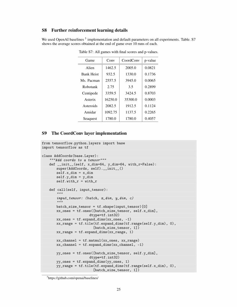
We used OpenAI baselines 5 implementation and default parameters on all experiments. Table. S7shows the average scores obtained at the end of game over 10 runs of each.

Table S7: All games with final scores and p-values.

Game Conv CoordConv p-value

Alien 1462.5 2005.0 0.0821

Bank Heist 932.5 1330.0 0.1736

Ms. Pacman 2557.5 3945.0 0.0065

Robotank 2.75 3.5 0.2899

Centipede 3359.5 3424.5 0.8703

Asterix 16250.0 35300.0 0.0003

Asteroids 2082.5 1912.5 0.1124

Amidar 1092.75 1137.5 0.2265

Seaquest 1780.0 1780.0 0.4057

S9 The CoordConv layer implementation

from tensorflow.python.layers import baseimport tensorflow as tf

class AddCoords(base.Layer):"""Add coords to a tensor"""def __init__(self, x_dim=64, y_dim=64, with_r=False):

super(AddCoords, self).__init__()self.x_dim = x_dimself.y_dim = y_dimself.with_r = with_r

def call(self, input_tensor):"""input_tensor: (batch, x_dim, y_dim, c)"""batch_size_tensor = tf.shape(input_tensor)[0]xx_ones = tf.ones([batch_size_tensor, self.x_dim],

dtype=tf.int32)xx_ones = tf.expand_dims(xx_ones, -1)xx_range = tf.tile(tf.expand_dims(tf.range(self.y_dim), 0),

[batch_size_tensor, 1])xx_range = tf.expand_dims(xx_range, 1)

xx_channel = tf.matmul(xx_ones, xx_range)xx_channel = tf.expand_dims(xx_channel, -1)

yy_ones = tf.ones([batch_size_tensor, self.y_dim],dtype=tf.int32)

yy_ones = tf.expand_dims(yy_ones, 1)yy_range = tf.tile(tf.expand_dims(tf.range(self.x_dim), 0),

[batch_size_tensor, 1])

5https://github.com/openai/baselines/

25

yy_range = tf.expand_dims(yy_range, -1)

yy_channel = tf.matmul(yy_range, yy_ones)yy_channel = tf.expand_dims(yy_channel, -1)

xx_channel = tf.cast(xx_channel, ’float32’) / (self.x_dim - 1)yy_channel = tf.cast(yy_channel, ’float32’) / (self.y_dim - 1)xx_channel = xx_channel*2 - 1yy_channel = yy_channel*2 - 1

ret = tf.concat([input_tensor,xx_channel,yy_channel], axis=-1)

if self.with_r:rr = tf.sqrt( tf.square(xx_channel)

+ tf.square(yy_channel))

ret = tf.concat([ret, rr], axis=-1)

return ret

class CoordConv(base.Layer):"""CoordConv layer as in the paper."""def __init__(self, x_dim, y_dim, with_r, *args, **kwargs):

super(CoordConv, self).__init__()self.addcoords = AddCoords(x_dim=x_dim,

y_dim=y_dim,with_r=with_r)

self.conv = tf.layers.Conv2D(*args, **kwargs)

def call(self, input_tensor):ret = self.addcoords(input_tensor)ret = self.conv(ret)return ret

26