and Physics Uncertainties and assessments of chemistry ...

Atmos. Chem. Phys., 3, 1–27, 2003www.atmos-chem-phys.org/acp/3/1/ Atmospheric

Chemistryand Physics

Uncertainties and assessments of chemistry-climate models of thestratosphere

J. Austin1, D. Shindell2, S. R. Beagley3, C. Bruhl4, M. Dameris5, E. Manzini6, T. Nagashima7, P. Newman8,S. Pawson8, G. Pitari9, E. Rozanov10, C. Schnadt5, and T. G. Shepherd11

1Meteorological Office, London Rd., Bracknell, Berks., RG12 2SZ, UK2NASA-Goddard Institute for Space Studies, 2880 Broadway, New York, NY 10025, USA3York University, Canada4Max Planck Institut fur Chemie, Mainz, Germany5DLR, Oberpfaffenhofen, Weßling, Germany6Max Planck Institut fur Meteorologie, Hamburg, Germany7Center for Climate System Research, University of Tokyo, Japan8Goddard Earth Sciences and Technology Center, NASA/Goddard Space Flight Center Code 916, Greenbelt, MD 20771,USA9Dipartamento di Fisica, Universita de L’Aquila, 67010 Coppito, L’Aquila, Italy10PMOD-WRC/ IAC ETH, Dorfstrasse 33, Davos Dorf CH-7260, Switzerland11Department of Physics, University of Toronto, Toronto, Ontario, Canada

Received: 28 May 2002 – Published in Atmos. Chem. Phys. Discuss.: 12 July 2002Revised: 9 September 2002 – Accepted: 24 September 2002 – Published: 9 January 2003

Abstract. In recent years a number of chemistry-climatemodels have been developed with an emphasis on the strato-sphere. Such models cover a wide range of time scales ofintegration and vary considerably in complexity. The resultsof specific diagnostics are here analysed to examine the dif-ferences amongst individual models and observations, to as-sess the consistency of model predictions, with a particularfocus on polar ozone. For example, many models indicatea significant cold bias in high latitudes, the “cold pole prob-lem”, particularly in the southern hemisphere during winterand spring. This is related to wave propagation from the tro-posphere which can be improved by improving model hori-zontal resolution and with the use of non-orographic gravitywave drag. As a result of the widely differing modelled polartemperatures, different amounts of polar stratospheric cloudsare simulated which in turn result in varying ozone values inthe models.

The results are also compared to determine the possiblefuture behaviour of ozone, with an emphasis on the polarregions and mid-latitudes. All models predict eventual ozonerecovery, but give a range of results concerning its timing andextent. Differences in the simulation of gravity waves andplanetary waves as well as model resolution are likely majorsources of uncertainty for this issue. In the Antarctic, theozone hole has probably reached almost its deepest although

Correspondence to:J. Austin ([email protected])

the vertical and horizontal extent of depletion may increaseslightly further over the next few years. According to themodel results, Antarctic ozone recovery could begin any yearwithin the range 2001 to 2008.

The limited number of models which have been integratedsufficiently far indicate that full recovery of ozone to 1980levels may not occur in the Antarctic until about the year2050. For the Arctic, most models indicate that small ozonelosses may continue for a few more years and that recoverycould begin any year within the range 2004 to 2019. Thestart of ozone recovery in the Arctic is therefore expected toappear later than in the Antarctic.

Further, interannual variability will tend to mask the signalfor longer than in the Antarctic, delaying still further the dateat which ozone recovery may be said to have started. Be-cause of this inherent variability of the system, the decadalevolution of Arctic ozone will not necessarily be a direct re-sponse to external forcing.

1 Introduction

The extent to which stratospheric change can influence cli-mate is only beginning to be understood. Before the dis-covery of the Antarctic ozone hole (Farman et al., 1985)it was thought that increases in the concentration of CO2

c© European Geosciences Union 2003

2 J. Austin et al.: Chemistry-climate models of the stratosphere

would cool the stratosphere and increase ozone (e.g. Grovesand Tuck, 1980). More generally it is now recognisedthat increases in the other well-mixed greenhouse gases(WMGHGs), CH4, N2O and chlorofluorocarbons, also coolthe stratosphere slightly. In polar regions, an increase inWMGHGs may increase Polar Stratospheric Clouds (PSCs)and decrease ozone in the Arctic (Austin et al., 1992) viathe same processes which produce the Antarctic ozone hole(Solomon, 1986). Changes to the thermal structure of thestratosphere also affect the wind fields which determine thetransport of ozone and the long-lived species that chemicallycontrol ozone. Decreases in stratospheric ozone change tro-pospheric chemistry by increasing the amount of UV radia-tion reaching the troposphere, and also cool the troposphereas ozone is itself a greenhouse gas. Consequently, atmo-spheric chemistry and climate are coupled in important ways.However, the degree of coupling is unclear. For example,Austin et al. (1992) showed that a doubling of CO2 concen-trations, expected towards the end of the 21st century, couldlead to severe Arctic ozone loss if large halogen abundancespersisted until that time.

On the other hand, the calculations of Pitari et al. (1992)showed only a slight reduction in Arctic ozone due to a CO2doubling, while again keeping halogen amounts fixed.

Since the early 1990s, the amendments to the MontrealProtocol have resulted in a considerable constraint on theevolution of halogen amounts and more recent calculationshave been able to take this into consideration. For exam-ple, in a coupled chemistry-climate simulation, Shindell etal. (1998a) calculated much increased ozone depletion overthe next decade or so, with severe ozone loss in the Arcticin some years. In contrast, recent results from other mod-els (Austin et al., 2000; Bruhl et al., 2001; Nagashima et al.,2002; Schnadt et al., 2002) indicate a relatively small changein Arctic ozone over the next few decades. The net effect onozone and temperature is that due to both the increased radia-tive cooling from WMGHG increases and due to changes indownwelling (and adiabatic warming) from planetary wavedrag. The latter changes could decrease ozone if planetarywave activity decreases, thus enhancing the radiative signal;or if planetary wave activity increases, the radiative signalcould be damped or even reversed causing an increase inozone. This illustrates one of the problems concerning futurepredictions: the simulation of the north polar stratospherictemperature, and thus ozone, is complicated by the mod-els’ ability to reproduce realistically the dynamical activityof this region. The model results therefore crucially dependon the length of the numerical simulation and model configu-ration, such as spatial resolution, position of the model upperboundary, gravity wave drag (gwd) scheme and the degreeof coupling between the chemically active species and theradiation scheme. The fact that the results are model depen-dent emphasises that the various dynamical-chemical feed-back mechanisms in the atmosphere, as well as the dynam-ical coupling between troposphere and stratosphere, are not

yet fully understood.These mechanisms are here explored by comparing spe-

cific diagnostics from a range of coupled chemistry-climatemodels. The primary interest is polar ozone and factors thatcontrol it, such as PSCs. Via transport, polar ozone alsohas an impact on middle latitudes which are also consid-ered briefly. In Sect. 2, the models are described and inSect. 3, model diagnostics are compared amongst the modelsand with observations. Having established model strengthsand weaknesses, their results are assessed in Sect. 4, to tryto provide a consensus on the likely trend in future ozone.Conclusions are drawn in Sect. 5.

2 Models used in the comparisons

Climate models have in the past been run with fixedWMGHGs for both present and doubled CO2 with the in-vestigation of the subsequent “equilibrium climate”. Severalcoupled chemistry-climate runs have followed this route withmulti-year “time slice” simulations applicable to WMGHGconcentrations for specific years (e.g. Rozanov et al., 2001;Schnadt et al., 2002; Pitari et al., 2002; Steil et al., 2002).Other climate simulations have involved transient changes inthe WMGHGs, and several coupled chemistry-climate sim-ulations have followed this pattern (Shindell et al., 1998a;Austin, 2002; Nagashima et al., 2002). The advantage oftransient experiments is that the detailed evolution of ozonecan be determined in the same way that it is likely to oc-cur (in principle) in the atmosphere, albeit with some sta-tistical error. The impact of interannual variability can beassessed by determining this variability over, e.g. a 10-yearperiod. Comparisons with observations are more direct sincethe concentrations of the halogens and WMGHGs are chang-ing to the same extent in the model as in the atmosphere.Time slice simulations need a sufficient duration (at least 10and preferably 20 years) to allow the interannual variabilityto be determined, but in principle, 20-year evaluations of thesame conditions may have less variability than the same pe-riod in the atmosphere in which halogens may be changingrapidly. Time slice runs also have the advantage that severalrealisations of the same year are available, from which futurepredictions can be assessed. However, in practice it may bebetter to examine the behaviour of different models, since agiven model will tend to have systematic errors. Both tran-sient simulations and time slice simulations are here used, tobring together the best of both sets of simulations.

The models used in the comparisons are indicated in Ta-ble 1, in order of decreasing horizontal resolution. All themodels have a comprehensive range of chemical reactionsexcept that in theGISSmodel the chemistry is parameterised.ULAQ is the only model with a substantial aerosol packagebut has diurnally averaged chemistry. This model has beenrun in time slice mode. Of the other models run in this mode,CMAM and MAECHAM/CHEMhave a high upper bound-

Atmos. Chem. Phys., 3, 1–27, 2003 www.atmos-chem-phys.org/acp/3/1/

J. Austin et al.: Chemistry-climate models of the stratosphere 3

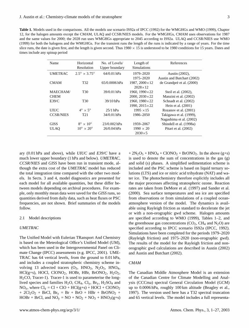
Table 1. Models used in the comparisons. All the models use scenario IS92a of IPCC (1992) for the WMGHGs and WMO (1999), Chapter12, for the halogen amounts except the CMAM, ULAQ and CCSR/NIES models. For the WMGHGs, CMAM uses observations for 1987and the same values for 2000; the 2028 run uses WMGHGs appropriate to 2045 according to IS92a. ULAQ and CCSR/NIES use WMO(1999) for both the halogens and the WMGHGs. For the transient runs the length of the runs is indicated by a range of years. For the timeslice runs, the date is given first, and the length is given second. Thus 1980× 15 is understood to be 1980 conditions for 15 years. Dates andtimes include any spinup period

Name Horizontal No. of Levels/ Length of ReferencesResolution Upper boundary Simulations

UMETRAC 2.5◦× 3.75◦ 64/0.01 hPa 1979–2020 Austin (2002),

1975–2020 Austin and Butchart (2002)CMAM T32 65/0.0006 hPa 1987, 2000×12 de Grandpre et al. (2000)

2028×12MAECHAM/ T30 39/0.01 hPa 1960, 1990×22 Steil et al. (2002),CHEM 2000, 2030×22 Manzini et al. (2002)E39/C T30 39/10 hPa 1960, 1980×22 Schnadt et al. (2002)

1990, 2015×22 Hein et al. (2001)UIUC 4◦

× 5◦ 25/1 hPa 1995×15 Rozanov et al. (2001)CCSR/NIES T21 34/0.01 hPa 1986–2050 Takigawa et al. (1999),

Nagashima et al. (2002)GISS 8◦ × 10◦ 23/0.002 hPa 1959–2067 Shindell et al. (1998a)ULAQ 10◦

× 20◦ 26/0.04 hPa 1990× 20 Pitari et al. (2002)2030×5

ary (0.01 hPa and above), whileUIUC and E39/C have amuch lower upper boundary (1 hPa and below).UMETRAC,CCSR/NIESandGISShave been run in transient mode, al-though the extra cost of theUMETRACmodel has reducedthe total integration time compared with the other two mod-els. In Sects. 3 and 4, model diagnostics are presented foreach model for all available quantities, but these differ be-tween models depending on archival procedures. For exam-ple, only monthly mean data were saved for theGISSruns, soquantities derived from daily data, such as heat fluxes or PSCfrequencies, are not shown. Brief summaries of the modelsfollow.

2.1 Model descriptions

UMETRAC

The Unified Model with Eulerian TRansport And Chemistryis based on the Meteological Office’s Unified Model (UM),which has been used in the Intergovernmental Panel on Cli-mate Change (IPCC) assessments (e.g. IPCC, 2001). UME-TRAC has 64 vertical levels, from the ground to 0.01 hPa,and includes a coupled stratospheric chemistry scheme in-volving 13 advected tracers (O3, HNO3, N2O5, HNO4,HCl(g+s), HOCl, ClONO2, HOBr, HBr, BrONO2, H2O2,H2CO, Tracer-1). Tracer-1 is used to parameterise the long-lived species and families H2O, CH4, Cly, Bry, H2SO4 andNOy, where Cly = Cl + ClO + HCl(g+s) + HOCl + ClONO2+ 2Cl2O2 + BrCl, Bry = Br + BrO + HBr + BrONO2 +HOBr + BrCl, and NOy = NO + NO2 + NO3 + HNO3(g+s)

+ 2N2O5 + HNO4 + ClONO2 + BrONO2. In the above (g+s)is used to denote the sum of concentrations in the gas (g)and solid (s) phases. A simplified sedimentation scheme isincluded and the PSC scheme is based on liquid ternary so-lutions (LTS) and ice or nitric acid trihydrate (NAT) and wa-ter ice. The photochemistry therefore explicitly includes allthe major processes affecting stratospheric ozone. Reactionrates are taken from DeMore et al. (1997) and Sander et al.(2000). Sea surface temperatures and sea ice are specifiedfrom observations or from simulations of a coupled ocean-atmosphere version of the model. The dynamics is avail-able using Rayleigh friction as standard to decelerate the jetor with a non-orographic gwd scheme. Halogen amountsare specified according to WMO (1999), Tables 1–2, andthe greenhouse gas concentrations (CO2, CH4 and N2O) arespecified according to IPCC scenario IS92a (IPCC, 1992).Simulations have been completed for the periods 1979–2020(Rayleigh friction) and 1975–2020 (non-orographic gwd).The results of the model for the Rayleigh friction and non-orographic gwd calculations are described in Austin (2002)and Austin and Butchart (2002).

CMAM

The Canadian Middle Atmosphere Model is an extensionof the Canadian Centre for Climate Modelling and Anal-ysis (CCCma) spectral General Circulation Model (GCM)up to 0.0006 hPa, roughly 100 km altitude (Beagley et al.,1997). The version used here has a T32 spectral truncationand 65 vertical levels. The model includes a full representa-

www.atmos-chem-phys.org/acp/3/1/ Atmos. Chem. Phys., 3, 1–27, 2003


tion of stratospheric chemistry with all the relevant catalyticozone loss cycles (de Grandpre et al., 1997). There are 31non-advected species and 16 advected species and familiesHNO4, HBr, CO, H2, CH3Br, CH4, N2O, H2O, CFC-11,CFC-12, Ox (= O(1D) + O(3P) + O3), NOx (= NO + NO2+ NO3 + 2N2O5), ClOx (= ClO + OClO + HOCl + Cl +ClONO2 + 2Cl2O2 + 2Cl2 + HCl(g+s)), BrOx (= Br + BrO +BrCl + BrONO2 + HOBr), HOx (= OH + HO2 + H + 2H2O2),and HNO3 (g+s). Chemical transport is accomplished usingspectral advection. Heterogeneous reactions are included forsulphate aerosols, LTS, and water ice, without sedimentation.

There is currently no parameterization of NAT PSCs, orof any associated denitrification. PSC threshold temper-atures are not adjusted to compensate for temperature bi-ases. Chemical reaction rates follow DeMore et al. (1997)and Sander et al. (2000). The chemistry is fully interactivewith the radiation code (de Grandpre et al., 2000). For theseruns, gravity wave drag is parameterised with the McFarlaneorographic scheme and the Hines non-orographic scheme(McLandress, 1998; Beagley et al., 2000).

The time-slice experiments are performed for 12 years,with the first two years discarded. Halogens are specifiedfrom WMO (1999), Chapter 12, and are identical in the 1987and 2028 runs. For the 1987 and 2000 runs, WMGHGs(CO2, CH4 and N2O) are specified from observations as of1987, and the sea surface temperatures and sea-ice distribu-tions are taken from Shea et al. (1990). For the 2028 run,WMGHGs are taken from the IPCC IS92a scenario whilesea-surface temperatures and sea-ice distributions are alteredaccording to the anomalies predicted from a transient simu-lation with the CCCma coupled climate model (Boer et al.,2000); however due to an error in the specification of the ex-periments, these forcings are appropriate to 2045 rather than2028.

MAECHAM/CHEM

This is a coupled chemistry-climate model based on the MA-ECHAM4 climate model. The chemistry module (Steil et al.,1998) adopts the “family” technique allowing time steps tobe as large as 45 min and includes reactive chlorine, nitro-gen and hydrogen, and methane oxidation. Photolysis ratesare calculated on-line using the fast and accurate scheme ofLandgraf and Crutzen (1998) to account for varying cloudsand overhead ozone.

Heterogeneous reactions on NAT and ice PSCs, and onsulphate aerosol are included, as well as sedimentation of icePSC particles. Since it is assumed that ice grows on NATparticles, this accounts to some extent for denitrification ifit is cold enough for ice. NAT PSCs are calculated fromthe model temperature, H2O and HNO3 using the formu-lae of Hanson and Mauersberger (1988), without assuminga nucleation barrier arguing that subgrid scale temperaturefluctuations produce the required supercooling. The grav-ity wave parameterization consists of two parts, separately

representing momentum flux deposition due to orographicgravity waves and a broad band spectrum of non-orographicgravity waves (Manzini and McFarlane, 1998). A modifiedversion of the McFarlane (1987) parameterization is used toaccount for the orographic gwd.

Chemical species are advected using the fluxform semi-Lagrangian transport scheme of Rasch and Lawrence (1998).For the time slice experiments the model is integrated about22 years (including spinup) using fixed surface mixing ratiosof source gases (WMO, 1999) and ten years average seasonalsea surface temperture distributions based on Hadley Centredata. For the simulations of future conditions, the averagesea surface temperatures have been taken from the transientclimate simulation of Roeckner et al (1999).

E39/C

A detailed description of this chemistry-climate model, alsoknown asECHAM4.L39(DLR)/CHEM, has been given byHein et al. (2001), who also discussed the main featuresof the model climatology. The model horizontal resolutionis T30 with a corresponding Gaussian transform latitude-longitude grid of mesh size 3.75◦

× 3.75◦ on which modelphysics, chemistry, and tracer transport are calculated. Themodel has 39 layers from the surface to the top layer cen-tred at 10 hPa (Land et al., 1999) and has particularly highresolution near the tropopause. A parameterization for oro-graphic gwd (Miller et al., 1989) is employed, but the ef-fects of non-orographic gravity waves are not considered.The chemistry module CHEM (Steil et al., 1998, updatedHein et al., 2001) uses reaction rate coefficients from De-More et al. (1997) and is based on the family concept, con-taining the most relevant chemical compounds and reactionsnecessary to simulate upper tropospheric and lower strato-spheric ozone chemistry, including heterogeneous chemicalreactions on PSCs and sulphate aerosol, as well as tropo-spheric NOx − HOx − CO− CH4 − O3 chemistry. The ad-vected tracers are CH4, HCl, H2O2, CO, CH3O2H, ClONO2,Ox (= O(1D) + O(3P) + O3), NOx (= N + NO + NO2 + NO3+ 2N2O5 + HNO4), ClOx (= Cl + ClO + HOCl), HNO3+ NAT and H2O + ICE. Physical, chemical, and transportprocesses are calculated simultaneously at each time step,which is fixed to 30 min. The PSCs in the model are basedon NAT and ice amounts depending on the temperature andthe concentration of HNO3 and H2O (Hanson and Mauers-berger, 1988). A nucleation barrier is prescribed to accountfor the observed super-saturation of NAT-particles (Schlageret al., 1990; Peter et al., 1991; Dye et al., 1992). A simpli-fied scheme for the sedimentation of NAT and ice particlesis applied. Stratospheric sulphuric acid aerosol surface ar-eas are based on background conditions (WMO, 1992, Chap-ter 3) with a coarse zonal average. Sea surface temperatureand sea ice distributions are prescribed for the various time



slices according to the greenhouse gas driven transient cli-mate change simulations of Roeckner et al. (1999).

UIUC

The University of Illinois at Urbana-Champaign model isa grid-point GCM with interactive chemistry (Yang et al.,2000; Rozanov et al., 2001). The model horizontal resolu-tion is 4◦ latitude and 5◦ longitude, with 24 layers spanningthe atmosphere from the surface to 1 hPa. The chemical-transport part of the model simulates the time-dependentthree-dimensional distributions of 42 chemical species (O3,O(1D), O(3P), N, NO, NO2, NO3, N2O5, HNO3, HNO4,N2O, H, OH, HO2, H2O2, H2O, H2, Cl, ClO, HCl, HOCl,ClONO2, Cl2, Cl2O2, CF2Cl2, CFCl3, Br, BrO, BrONO2,HOBr, HBr, BrCl, CBrF3, CH3Br, CO, CH4, CH3, CH3O2,CH3OOH, CH3O, CH2O, and CHO), which are determinedby 199 gas-phase and photolysis reactions. The modelalso takes into account 6 heterogeneous reactions on andin sulphate aerosol and polar stratospheric cloud particles.The chemical solver is based on the pure implicit iterativeNewton-Raphson scheme (Rozanov et al., 1999). The re-action coefficients are taken from DeMore et al. (1997) andSander et al. (2000).

Photolysis rates are calculated at every chemical step us-ing a look-up-table (Rozanov et al., 1999). The advectivetransport of species is calculated using the hybrid advec-tion scheme proposed by Zubov et al. (1999). A simpli-fied scheme is applied for the calculation of the PSC parti-cles (NAT and ice) formation and sedimentation. Sea surfacetemperature and sea ice distributions are prescribed from theAMIP-II monthly mean distributions, which are the averagesfrom 1979 through 1996 (Gleckler, 1996). The orographicscheme of Palmer et al. (1986) is used to parameterise grav-ity wave drag.

In this paper the results of a 15-year long control run ofthe model will be considered. The climatology of this runhas been presented by Rozanov et al. (2001).

CCSR/NIES

An overview of the Center for Climate System Re-search/National Institute for Environmental Studies GCMwith an interactive stratospheric chemistry module has beendescribed in Takigawa et al. (1999), and some updates for thepresent integration are given by Nagashima et al. (2002). Thehorizontal resolution is T21 (longitude× latitude' 5.6◦

×

5.6◦) and the vertical domain extends from the surface toabout 0.01 hPa with 34 layers. Orographic gwd is parame-terised following McFarlane (1987), but non-orographic gwdis not included. In the model, 19 species and 5 chemical fam-ilies are explicitly transported: CH4, N2O, H2O2, H2O(g+s),HNO3 + NAT, HNO4, N2O5, ClONO2, HCl, HOCl, Cl2,ClNO2, CCl4, CFC11, CFC12, CFC113, HCFC22, CH3Cl,CH3CCl3, Ox, HOx (= H + OH +HO2), NOx(= N + NO

+NO2 + NO3), ClOx (= Cl + ClO + ClOO + Cl2O2), NOyand Cly. The amount of NAT and ice PSCs are calculated us-ing the relationship of Hanson and Mauersberger (1988) andof Murray (1967), respectively. As in E39/C, a nucleationbarrier is also assumed.

Reaction rate coefficients are taken primarily fromDeMore et al. (1997) and Sander et al. (2000). A 65-yeartransient integration was performed for the period 1986–2050 including the trends of chlorine-containing substances(WMO, 1999, Table 12-2) and those of greenhouse gases(Also WMO, 1999, Table 12-2, very similar to IPCCscenario IS92a, IPCC, 1992). The expected sea surface tem-perature variation, separately calculated by the CCSR/NIEScoupled ocean-atmospheric GCM, is also applied.

GISS

The model used here is a version of the Goddard Institutefor Space Studies stratospheric climate model which has8◦

× 10◦ horizontal resolution, and 23 vertical layers ex-tending up into the mesosphere (top at 0.002 hPa,∼ 85 km)(Rind et al., 1988a, b). This atmospheric model is coupledto a mixed-layer ocean, allowing sea surface temperaturesto respond to external forcings. A gravity wave parameter-ization is employed in the model in which the temperatureand wind fields in each grid box are used to calculate gravitywave effects due to wind shear, convection, and topography.For the runs described here, the mountain drag was set toone quarter the original value which gives a better reproduc-tion of observed temperatures in the polar lower stratosphereof each hemisphere during their respective winter and springperiods. The model includes a simple parameterization ofthe heterogeneous chemistry responsible for polar ozone de-pletion (Shindell et al., 1998a). Chlorine activation takesplace whenever temperatures fall below 195 K. Ozone de-pletion is then calculated at each location with active chlo-rine and sunlight using the reaction rates of DeMore et al.(1997). An additional contribution of 15% from brominechemistry is also included. When heterogeneous process-ing ceases, chlorine deactivation follows two-dimensionalmodel-derived rates (Shindell et al., 1998b). Ozone recov-ery rates are parameterised so that ozone losses are restoredbased on the photochemical lifetime of ozone at each alti-tude. Changes in ozone transport are not included interac-tively, but are calculated after the model runs and included inthe results shown here. The model was run with increasinggreenhouse gas concentrations starting in 1959 and continu-ing until 2067. The trends in greenhouse gas concentrationswere based on observations until 1985, and subsequently fol-lowed the IPCC projections IS92a (IPCC, 1992), althoughthe observed rates of increase since 1985 have been some-what less.



J.Austinet al.: Chemistry-climatemodelsof thestratosphere 23

Fig. 1. Monthly meantotal ozone(DU) over thenorthernhemispherefor themonthof March for thecurrentatmospherefor participatingmodels.Theobservationsaretakenfrom arangeof satellitedata(seetext) for theperiod1993–2000.Themodelclimatologiesareasfollows:UMETRAC: mean1980–2000,CMAM: 2000run,MAECHAM/CHEM: 2000run,E39/C:1990run,CCSR/NIES:mean1990–1999,UIUC:1995run,ULAQ, 1990run.

www.atmos-chem-phys.org/0000/0001/ Atmos.Chem.Phys.,0000,0001–34,2002

Fig. 1. Monthly mean total ozone (DU) over the northern hemisphere for the month of March for the current atmosphere for participatingmodels. The observations are taken from a range of satellite data (see text) for the period 1993–2000. The model climatologies are as follows:UMETRAC: mean 1980–2000, CMAM: 2000 run, MAECHAM/CHEM: 2000 run, E39/C: 1990 run, CCSR/NIES: mean 1990–1999, UIUC:1995 run, ULAQ, 1990 run.

ULAQ

The University of L’Aquila model is a low-resolution cou-pled chemistry-climate model, which has been extensivelyused in the IPCC assessment (IPCC, 2001). The chemical-transport module has a resolution of 10◦

× 20◦ in latitude-longitude. There are 26 log-pressure levels, from the groundto about 0.04 hPa, giving an approximate vertical resolutionof 2.8 km. Dynamical fields (streamfunction, velocity poten-tial and temperature) are taken from the output of a spec-tral GCM (Pitari et al., 2002). Vertical diffusion is used tosimulate those processes not explicitly included in the modelsuch as the effect of breaking gravity waves. See Pitari et al.(1992) and Pitari et al. (2002) for further details of the model.

The Chemical Transport Model (CTM) and GCM are cou-pled via the dynamical fields and via the radiatively activespecies (H2O, CH4, N2O, CFCs, O3, NO2, and aerosols).All chemical species are diurnally averaged. The mediumand short-lived chemical species are grouped into families:Ox, NOx, NOy (= NOx + HNO3), HOx, CHOx, Cly, Bry,SOx and aerosols. The long-lived and surface-flux species inthe model are N2O, CH4, H2O, CO, NMHC, CFCs, HCFCs,halons, OCS, CS2, DMS, H2S, SO2 for a total of 40 trans-ported species (plus 57 aerosol size categories) as well as26 species at photochemical equilibrium. All photochemi-cal data are taken from DeMore et al. (1997), including themost important heterogeneous reactions on sulphate and PSCaerosols. The ULAQ model also includes the most important



tropospheric aerosols. The size distribution of sulphate (bothtropospheric and stratospheric) and PSC aerosols, treated asNAT and water ice, are calculated using a fully interactiveand mass conserving microphysical code for aerosol forma-tion and growth. Denitrification and dehydration due to PSCsedimentation are calculated explicitly from the NAT and iceaerosol predicted size distribution. WMGHG and halogenscenarios are taken from WMO (1999).

Changes in surface fluxes of CO, NOx, non-methanehydrocarbons, SOx and carbonaceous aerosols are takenfrom IPCC (2001). Climatological sea surface temperatures(SSTs) are used for present day conditions, and a simple heatsource model is used to estimate the change in SSTs for fu-ture conditions.

2.2 Model ozone climatologies for the current atmosphere

To put the subsequent model results into context, we firstcompare the ozone climatologies from the different modelsduring spring with the corresponding satellite observationsfor the years 1993–2000 (see Rozanov et al., 2001 for a de-scription of the data included). The geographical distribu-tion of the monthly mean total ozone over the northern hemi-sphere in March and over the southern hemisphere in Octo-ber are presented in Figs. 1 and 2 for the data and partici-pating models. The hemispheric area weighted total ozoneis presented on Table 2. The table also includes the patterncorrelation coefficients between the observed and simulatedtotal ozone fields, defined as the correlation coefficient be-tween observations and model over all the grid points withequal area weighting. TheGISSmodel results are not shownin this section, as the chemistry parameterization is a pertur-bation from the observed climatology.

In the northern hemisphere (Fig. 1), all the models simu-late the position and intensity of the primary total ozone max-imum reasonably well. However,UMETRAC, CCSR/NIES,E39/C and CMAM models slightly overestimate the exten-sion of the ozone maximum area. In these models the areawhere total ozone is higher than 425 DU covers a substantialpart of Siberia and spreads to northern Canada. Total ozonein MAECHAM/CHEMis higher than observed values overthe entire hemisphere. The area of ozone maximum in theUIUC andULAQmodels extends to the Pacific sector, whichimplies an underestimated intensity of the Aleutian highs inthe stratosphere. This dynamical feature also leads to theequatorward shift of the area with elevated total ozone in thePacific sector. TheCCSR/NIESmodel simulates very wellthe magnitude of the primary maximum, although its posi-tion is slightly shifted to the west. This shift, and the shape ofthe 400 DU contour imply that the intensity of the Aleutianmaximum in theCCSR/NIESmodel is overestimated. Thesimulated position and magnitude of the elevated total ozoneover northern Canada are in good agreement with observa-tions. However, in most of the participating models this areais shifted to the north and its magnitude is slightly overesti-

Table 2. Simulated and observed area weighted total ozone andpattern correlation coefficients between total ozone fields.1 is thequantity (model – observations)/observations

March, NH Total Ozone 1 (%) Correlation

Observations 318.0 – –UMETRAC 339.9 +6.9 0.98CMAM 338.0 +6.3 0.97MAECHAM/CHEM 371.8 +16.9 0.95E39/C 351.2 +10.4 0.98UIUC 322.6 +1.4 0.84CCSR/NIES 326.1 +2.5 0.98ULAQ 337.6 +6.2 0.85

October, SH Total Ozone 1 (%) Correlation

Observations 291.1 – –UMETRAC 337.8 +16.0 0.86CMAM 324.3 +11.4 0.97MAECHAM/CHEM 349.0 +19.9 0.98E39/C 301.7 +3.6 0.97UIUC 277.2 −4.8 0.97CCSR/NIES 318.2 +9.3 0.95ULAQ 314.8 +8.1 0.94

mated, while theUIUC andULAQ models tend to shift thisarea to the south. In agreement with the observations the areawith rather low total ozone appears inUIUC, CCSR/NIES,MAECHAM/CHEMand E39/C models just over the NorthPole reflecting the position of the Polar vortex. However, thisfeature is not present in theUMETRAC, ULAQandCMAMtotal ozone maps. Table 2 shows that the overall perfor-mance of all the models in March over the northern hemi-sphere is reasonably good. The pattern correlation with ob-served data is greater than 0.95 forUMETRAC, CCSR/NIES,E39/C, CMAMandMAECHAM/CHEMmodels but a lowercorrelation occurs for theUIUC andULAQ models partiallybecause of the underprediction in the strength of the Aleutianhigh. All the models overestimate the area weighted hemi-spheric total ozone, by on average 7.2%.

Figure 2 shows the total ozone for the observations andmodels for the southern hemisphere in October. The patterncorrelations between simulated and observed total ozone (Ta-ble 2) are similar to that in the northern hemisphere.

UMETRAC, CCSR/NIES, MAECHAM/CHEM, ULAQandCMAM models noticeably overestimate the area weightedtotal ozone. This total ozone surplus comes from slightlyhigher total ozone in the tropics and from substantialoverestimation of the magnitude of the total ozone max-imum over the middle latitudes. For example the totalozone exceeds 475 DU in theUMETRACresults, 450 DUin MAECHAM/CHEMand 425 DU in theCCSR/NIES, andCMAMresults, while in the observations the total ozone peakjust exceeds 375 DU. From these results we can conclude ei-



24 J.Austin etal.: Chemistry-climatemodelsof thestratosphere

Fig. 2. As in Fig. 1, but for Octoberin theSouthernHemisphere.

Atmos.Chem.Phys.,0000,0001–34,2002 www.atmos-chem-phys.org/0000/0001/

Fig. 2. As in Fig. 1, but for October in the Southern Hemisphere.

ther that the meridional transport and wave forcing are over-estimated by these models, or that the vortex barrier is toostrong. For MAECHEM/CHEM, CCSR/NIES and CMAMthe cold-pole bias evident in Fig. 5 suggests that the latter ef-fect is definitely a factor. In contrast theE39/CandUIUCmodels, which are the two models with the lowest upperboundary, match the observed total ozone very closely. Theposition of the total ozone maximum over middle-latitudes isalso shifted from the Australian sector to the Indian Oceansector inUMETRACandCCSR/NIESmodels and to the Pa-cific Ocean sector in theUIUC model. The position andmagnitude of the ozone hole over the South Pole is well re-produced by the models, implying that the amount of PSCsduring the spring season and chemical ozone destruction arereasonably well captured by the chemical routines. This isdiscussed further in Sects. 3.2 and 4.4.

3 Model uncertainties

3.1 Temperature biases

Many climate models without chemistry but with a fully re-solved stratosphere have a cold bias of the order of 5–10 Kin high southern latitudes in the lower stratosphere, suggest-ing that the residual circulation is too weak (Pawson et al.,2000), i.e. there is too little downwelling in polar latitudesand too little upwelling in lower latitudes. This temperaturebias could have a significant impact on model heterogeneouschemistry, and enhance ozone destruction. The “cold poleproblem” extends to higher levels in the stratosphere andby the thermal wind relation gives rise typically to a polarnight jet that is too strong and which has an axis that doesnot slope with height, whereas in the observations the po-lar night jet axis slopes with height towards the equator in



Dec/Jan/Feb 80N�

−30� −20 −10 0� 10Model Temperature bias (K)

1000

300

100

30

10

3

1

Pre

ssur

e hP

a

�

Mar/Apr/May 80N

−30� −20 −10 0� 10Model Temperature bias (K)

1000

300

100

30

10

3

1

Pre

ssur

e hP

a

�

Jun/Jul/Aug 80S�

−30� −20 −10 0� 10Model Temperature bias (K) �

1000

300

100

30

10

3

1

Pre

ssur

e hP

a

�

Sep/Oct/Nov 80S�

−30� −20 −10 0� 10Model Temperature bias (K) �

1000

300

100

30

10

3

1

Pre

ssur

e hP

a�

_ _ _ UMETRAC Rayleigh friction____ UMETRAC Non−orographic GWD____ CMAM 2000 run____ MAECHAM/CHEM____ E39/C

____ CCSR/NIES_ _ _ UIUC____ ULAQ_ _ _ GISS

Fig. 3. Temperature biases at 80◦ N and 80◦ S for the winter and spring seasons, as a function of pressure. To determine the bias, aclimatology determined from 10 years of UKMO data assimilation temperatures was subtracted from the model results averaged for thesame years as indicated in Fig. 1.

the upper stratosphere. The weaker jet and slope of the axisallow waves to propagate into higher latitudes and maintainhigher polar temperatures. A potentially important compo-nent of climate change is whether these waves increase inamplitude with time since this will likely affect the evolu-tion of ozone: see Sect. 3.4. A practical solution for thosemodels with a cold bias is to adjust the temperatures in theheterogeneous chemistry (e.g. Austin et al., 2000) so that theheterogeneous chemistry is calculated using realistic temper-atures. The strong polar night jet is also associated with avortex that breaks down later in the spring, particularly in thesouthern hemisphere. In a chemistry-climate model this canlead to a longer lasting ozone hole. Adjusting model PSCthreshold temperatures to allow for model temperature bias

cannot solve this problem.

Recently the development of non-orographic gwd schemesfor climate models (Medvedev and Klaassen, 1995; Hines,1997; Warner and McIntyre, 1999) has resulted in a signif-icant reduction in the cold pole problem relative to simula-tions that rely on Rayleigh friction to decelerate the polarnight jet (e.g. Manzini and McFarlane, 1998). Two of theseschemes have also been shown to produce a quasi-biennialoscillation (QBO) when run in a climate model (Scaife et al.,2000, McLandress, 2002). The latest versions of several cou-pled chemistry-climate models now employ such schemes:CMAM uses the Medvedev-Klaassen scheme (Medvedev etal., 1998) or the Hines scheme (McLandress, 1998); the lat-est version of UMETRAC uses the Warner and McIntyre



26 J.Austin etal.: Chemistry-climatemodelsof thestratosphere

0¹ 5º 10 15 20 25Heat flux at 100 hPa, Jan and Feb mean»200

205

210

215

220

225

Mea

n T

empe

ratu

re F

eb a

nd M

arch

¼(a)½

(b)½

(c)½


205

210

215

220

225

Mea

n T

empe

ratu

re F

eb a

nd M

arch

¼

(a) Observations

(a)½

(b) UMETRAC Non−orographic gwd (c) CCSR/NIES

(f) ULAQ (g) CMAM 2000 run

(d) MA−ECHAM CHEM 1990 run

(d)½

(e) E39/C

(e)½


205

210

215

220

225

Mea

n T

empe

ratu

re F

eb a

nd M

arch

¼(a)½

(f)½

(g)½

Fig. 4. Scatterdiagramsof heatflux ¾�¿�«�¿ (averaged40� –80� N, at 100hPa for JanuaryandFebuary)againsttemperature(averaged60� –90� N, at 50 hPa for FebruaryandMarch) for participatingmodelsfor the sameyearsas indicatedin Fig. 1. The solid lines are linearregressionlinesbetweenthe two variables.Theobservationsaretaken from NCEPassimilations.Theheatflux is in unitsof Kms§G¨ , thetemperatureis in K.

Atmos.Chem.Phys.,0000,0001–34,2002 www.atmos-chem-phys.org/0000/0001/

Fig. 4. Scatter diagrams of heat fluxv′T ′ (averaged 40◦–80◦ N, at 100 hPa for January and Febuary) against temperature (averaged 60◦–90◦ N, at 50 hPa for February and March) for participating models for the same years as indicated in Fig. 1. The solid lines are linearregression lines between the two variables. The observations are taken from NCEP assimilations. The heat flux is in units of Kms−1, thetemperature is in K.

scheme; and MAECHAM/CHEM uses the Hines scheme(Manzini et al., 1997). The GISS GCM has used a non-orographic gwd scheme for many years (Rind et al., 1988a,b), which is able to reproduce high latitude temperatures rea-sonably well (Shindell et al., 1998b) but does not simulate aQBO in the tropics.

Figure 3 shows model temperature biases as a function ofheight for 80◦ N and 80◦ S for the winter and spring seasons.To determine the biases, a 10-year temperature climatol-ogy determined from data assimilation fields (Swinbank andO’Neill, 1994) was subtracted from the mean model temper-ature profiles applicable to the 1990s. The UKMO tempera-tures are considered to be typically about 2 K too high at lowtemperatures (e.g. Pullen and Jones, 1997). Although typicalmodel biases are somewhat larger than 2 K it is also possiblethat our climatology in the high latitude regions are less reli-able because of large interannual variability. The upper andmiddle stratospheric cold pole problem is particularly no-ticeable in the south in the UMETRAC (with Rayleigh fric-

tion), CCSR/NIES, E39/C and MAECHAM/CHEM results.With a non-orographic gwd scheme the temperature biasesreduce considerably and both CMAM and UMETRAC havevery similar results in the seasons analysed. In the UIUC,GISS and ULAQ models a warm bias is present in the mid-dle stratosphere in winter. For the latter models, which havelower horizontal resolution than the other five, the biases maybe a result of the need to adjust physical parameterizations toobtain improved climatologies and that such adjustments arenot always suitable for all seasons. The ULAQ model, forexample, includes vertical diffusion, in addition to Rayleighfriction. The MAECHAM/CHEM model uses the Hines non-orographic gwd scheme, but in southern winter the resultsare only a slight improvement on the Rayleigh friction re-sults of UMETRAC and CCSR/NIES. For other seasons,the MAECHAM/CHEM temperature bias is much smallerand is similar to the results of E39/C which has equivalentphysics and chemistry, but does not have a non-orographicgwd scheme. Nonetheless, Manzini et al. (1997) indicated



J.Austinet al.: Chemistry-climatemodelsof thestratosphere 27

0¹ 2À 4Á 6Â 8Ã 10 12Heat flux at 100 hPa, Jul and Aug mean»185

190

195

200

205

Mea

n T

empe

ratu

re A

ug a

nd S

ept

Ä (a)½

(b)½

(c)½

0¹ 2À 4Á 6Â 8Ã 10 12Heat flux at 100 hPa, Jul and Aug mean»185

190

195

200

205

Mea

n T

empe

ratu

re A

ug a

nd S

ept

Ä

(a) Observations

(a)½

(b) UMETRAC Non−orographic gwd (c) CCSR/NIES

(f) ULAQ (g) CMAM 2000 run

(d) MA−ECHAM CHEM 1990 run

(d)½

(e) E39/C

(e)½

0¹ 2 4 6Â 8Ã 10 12Heat flux at 100 hPa, Jul and Aug mean»185

190

195

200

205

Mea

n T

empe

ratu

re A

ug a

nd S

ept

Ä (a)½

(f)½

(g)½

Fig. 5. As in Fig. 4, but for the SouthernHemispherefor the monthsJuly and August, and August and September, respectively. Forconvenience,the usualconvention for ¾ hasbeenused(i.e. negative valuesindicate toward the SouthPole) but the valueshave beenmultipliedby ¦�¡ ).

www.atmos-chem-phys.org/0000/0001/ Atmos.Chem.Phys.,0000,0001–34,2002

Fig. 5. As in Fig. 4, but for the Southern Hemisphere for the months July and August, and August and September, respectively. Forconvenience, the usual convention forv has been used (i.e. negative values indicate toward the South Pole) but the values have been multipliedby −1).

that the temperature biases in the core climate model aresmaller when non-orographic gwd is included.

At 80◦ N temperature biases are generally somewhatsmaller than at 80◦ S and for some models are positive atsome levels. The northern lower stratospheric temperaturebiases would generally lead to insufficient heterogeneousozone depletion in early winter but excessive ozone depletionin the more important spring period. In the southern hemi-sphere, spring cold biases could lead to more extensive PSCsthan observed and delayed recovery in Antarctic ozone.

Newman et al. (2001) showed that the lower stratospherictemperature is highly correlated with the lower stratosphericheat fluxv′T ′ slightly earlier in the year. The heat flux pro-vides a measure of the wave forcing from the troposphere,and in Fig. 4, the heat flux at 100 hPa averaged over the do-main 40◦–80◦ N for January and February is plotted againsttemperature averaged over the domain 60◦–90◦ N at 50 hPafor February and March. Similar results for the southernhemisphere are shown in Fig. 5. Newman et al. choosethe period of the temperature average as 1–15 March, which

maximises the correlation coefficient between the two vari-ables at 0.85. However, here we choose a longer period forthe temperature average to smooth over any model and atmo-spheric transients. This reduces the correlation coefficient forNCEP data only slightly, to 0.77 (0.78 in the south). Table 3shows the correlation coefficient (R) between the two vari-ables, computed for data and model results within the period1980-2000.T0 is the temperature intercept at zero flux,β isthe gradient of the lines in Figs. 4 and 5, andσ is the standarddeviation in the computation ofβ. T0 indicates the radiativeequilibrium temperature, including a contribution from smallscale waves not represented in the heat flux (e.g. Newman etal., 2001).

In the north (Fig. 4), the model results are for the mostpart in reasonable agreement with the observations, althoughthe model correlation coefficients vary in the range 0.52 to0.86. Model horizontal resolution may have significantly af-fected the results: in general the model regression lines areless steep (smallerβ in Table 3) as the model resolution de-creases. This could be because while low-resolution models



Table 3. Statistical analysis of the linear regression between the area averaged temperature (K) at 50 hPa polewards of 60◦ N for Februaryand March, and the heat flux (Kms−1) at 100 hPa between 40◦ and 80◦ N for January and February (Northern Hemisphere). The SouthernHemisphere results are for the months August and September and July and August, respectively.R is the correlation coefficient between thevariables,T0 is the intercept of the line at zero heat flux,β is the gradient of the line andσ is the standard error in the computation ofβ

Model/Observations N’ern Hemi. S’ern Hemi.R T0 β σ R T0 β σ

NCEP (Observations) 0.77 195.1 1.49 0.27 0.78 189.4 0.89 0.16UMETRAC Non-orographic gwd 0.77 196.9 1.20 0.22 0.74 187.5 1.14 0.23

Rayleigh Friction 0.63 196.7 1.19 0.33 0.47 186.8 0.82 0.34CMAM 2000 0.52 204.5 0.75 0.43 0.44 191.3 0.68 0.50MAECHAM/CHEM 1990 0.83 190.4 1.47 0.23 0.72 188.8 0.45 0.10E39/C 0.62 198.3 0.93 0.28 0.86 186.3 0.56 0.08CCSR/NIES 0.86 199.2 0.86 0.14 0.66 187.4 0.98 0.29ULAQ 0.58 203.0 0.48 0.16 0.64 192.9 1.01 0.29

can capture the low-amplitude wave, small heat flux case,they may have more difficulty capturing the large heat fluxcase with its possibly significant potential enstrophy cascadeto larger wavenumbers. However, this covers a broad spec-trum of results. For example, CMAM simulates a wide rangeof heat fluxes consistent with observations but the functionalrelationship with temperature is highly sensitive to a singleyear’s data. Removal of the single point corresponding tothe highest heat flux, increases the correlation coefficient to0.67 and increasesβ to 1.06, much closer to that expected onthe basis of the model resolution. This implies that the 10-year CMAM run is too short to give fully meaningful resultsin the northern hemisphere for this diagnostic. The perfor-mance of the models might also depend on the dissipationthat the models have at short spatial scales, although this ismore difficult to compare.

In the southern hemisphere (Fig. 5) the correlation co-efficients cover the range 0.44 to 0.86, wider than in thenorth.T0 is considerably lower, probably due to lower ozoneamounts, and all the models agree well with the observedT0.For the time slice experiments (e.g. MAECHAM/CHEM)T0decreased from the 1960 results (not shown) to the 1990 re-sults due to the WMGHG increase and ozone depletion. Thevalues ofβ are also generally smaller in the southern hemi-sphere, except for the CCSR/NIES and ULAQ models. Un-like in the northern hemisphere, the model results indicatethat resolution is not a factor in the value ofβ. That is, bothlow and high resolution models are in principle capable ofcapturing the observed temperature-heat flux relationship.

3.2 The simulation of polar stratospheric clouds

During the last few years, considerable progress has beenmade regarding the understanding of PSCs and the associ-ated heterogeneous chemical reactions. Some of these de-velopments are discussed in Carslaw et al. (2001) and WMO(2002), Chapter 3. They include the observation of many

different types of PSCs, both liquid and solid forms, and thelaboratory measurement of a wide range of chemical reac-tion rates as summarised in Sander et al. (2000). Coupledchemistry-climate models have a variety of PSC schemeswith and without sedimentation, but as indicated in Sect. 3.1,some models have large climatological biases in the polar re-gions. If the models are to produce accurate simulations ofozone depletion, the temperature field must give realistic dis-tributions near the PSC temperature threshold. So that com-mon ground can be established between models, we here usethe temperature at 50 hPa as an indicator, hence ignoring theimpact of HNO3 and sulphate concentrations on the determi-nation of PSC surface areas.

Following Pawson and Naujokat (1997) and Pawson et al.(1999), Fig. 6 shows for each of the participating models andobservations the time integral throughout the winter of theapproximate PSC area at 50 hPa, as given by the areas withinthe 195 K and 188 K temperature contours. This is the quan-tity Aτ indicated in Fig. 9 of Pawson et al. (1999), but with-out the normalisation factor of 1/150, forτNAT = 195 K andτICE = 188 K. Aτ is here measured in terms of the frac-tion of the hemisphere covered in % times their duration indays. For the ice amount in the Arctic,Aτ varies dramati-cally between zero (ULAQ and CMAM models, not shown)and 215 (CCSR/NIES) in units of % of the hemisphere timesdays and the models have large interannual variability. Arc-tic NAT also covers a large range, both for different modelsand in the interannual variability for each simulation. In ac-cordance with their temperature biases, several models havelarger areas of NAT than are typically derived from observa-tions. The ULAQ PSCs are in good agreement with obser-vations, despite a slight temperature bias, while UMETRACand CMAM have lower PSCs than are derived from obser-vations. In the Antarctic most models have much lower frac-tional interannual variation, but again the results for separatemodels cover an exceedingly large range for the ice amount.ULAQ and UMETRAC are in good agreement with obser-



Arctic NAT�

1960 1980 2000 2020 year�

0

200

400

600

Sea

sona

l PS

C %

day

s�

Arctic ICE�

1960 1980 2000 2020 year�

0

50

100

150

200

250

Sea

sona

l PS

C %

day

s

�

Antarctic NAT�

1960 1980 2000 2020 year�

0

500

1000

1500

2000

Sea

sona

l PS

C %

day

s

�

Antarctic ICE�

1960 1980 2000 2020 year�

0

200

400

600

800

1000

Sea

sona

l PS

C %

day

s�

____Observations

_ _ _ UMETRAC Non−orographic GWD

MAECHAM/CHEM E39/CULAQ

�CMAM.......

CCSR/NIES

Fig. 6. Seasonal integration of the hemispheric area at 50 hPa, corresponding to the temperatures below 195 K (approximate NAT tempera-ture) and below 188 K (approximate ICE temperature) for participating models except E39/C which shows the actual PSC area. The errorbars for the time slice runs indicate 95% confidence intervals. For clarity, ULAQ data are plotted two years early, and for 1990 and 2030MAECHEM CHEM data are plotted two years late.

vations for both the NAT and ice temperature, but the othermodels tend to overpredict the PSC amounts. The implica-tions for ozone on the differences between the models is dis-cussed further in Sect. 4.4.

The sedimentation of PSC particles is now thought to beimportant in polar ozone depletion (e.g. Waibel et al., 1999),but is absent from many coupled chemistry-climate models.Using a 3-D model without transport, Waibel et al. (1999)suggested that cooling associated with greenhouse gas in-creases may lead to higher ozone depletion than if sedimen-tation were ignored. There are many practical difficulties as-sociated with incorporating sedimentation in climate models.The full details, including dividing the particles into differentsized bins (e.g. Timmreck and Graf, 2000), cannot be readilysimulated in most models as this would require the transport

of particles covering a large number of size ranges, whichmay exceed the total number of tracers transported. Whilethe ULAQ model (Pitari et al., 2002) is able to simulate thislevel of complexity, the model resolution is somewhat coarse(see Table 1). Most models therefore adopt some extremelysimplified procedures. For example in the UMETRAC model(Austin, 2002) sedimentation is assumed to occur for NATor ice particles of fixed size. The vertical transport equa-tion is solved locally to give a sedimented field which is notexplicitly advected horizontally but is tied to the field of aconserved horizontal tracer. Other models (e.g. Egorova etal., 2001; Hein et al., 2001; Pitari et al., 2002) transport thesedimented field in more detail, but the accuracy of this trans-port may be limited by model spatial resolution, and whetherit can treat small scale features with high enough precision.



DJF �

−90� −60� −30� 0� 30 60 90 Latitude

−4

−2

0

2

4

6

8

Str

eam

func

tion

at 5

0 hP

a 1.

0 e9

Kg/

s MAM�

−90� −60� −30� 0� 30 60 90 Latitude

−4

−2

0

2

4

6

Str

eam

func

tion

at 5

0 hP

a 1.

0 e9

Kg/

s

JJA�

−90� −60� −30� 0� 30 60 90 Latitude�

−6

−4

−2

0

2

4

Str

eam

func

tion

at 5

0 hP

a 1.

0 e9

Kg/

s

a

b

c

d

e f

SON�

−90� −60� −30� 0� 30 60 90 Latitude�

−4

−2

0

2

4

6

Str

eam

func

tion

at 5

0 hP

a 1.

0 e9

Kg/

s

(a) Observations (b) UMETRAC(c) MAECHAM/CHEM (d) E39/C(e) CCSR/NIES (f) GISS

Fig. 7. Residual streamfunction (109 Kgs−1) at 50 hPa as a function of latitude and season for the participating models.

Recently, the presence of large, nitric acid containing parti-cles exceeding 10µm in diameter has been detected in thelower stratosphere (Fahey et al., 2001). Models have onlyjust started to take the production of these particles into ac-count (Carslaw, personal communication, 2002), althoughthey may have an important impact on ozone depletion.

3.3 The transport of constituents

There is strong evidence from a number of modelling studies(Garcia and Boville, 1994; Shepherd et al., 1996; Lawrence,1997; Austin et al., 1997; Rind et al., 1998; Beagley et al.,2000) that the position of the model upper boundary can play

a significant role in influencing transport and stratosphericdynamics due to the “downward control principle” (Hayneset al., 1991). The sensitivity of the dynamical fields to theposition of the upper boundary may be more when usingnon-orographic gwd schemes than when Rayleigh frictionis used, although if all the non-orographic gwd that is pro-duced above the model boundary is placed instead in thetop model layer, this sensitivity reduces (Lawrence, 1997).Model simulations with an upper boundary as low as 10 hPahave been completed (e.g. Hein et al., 2001; Schnadt et al.,2002; Dameris et al., 1998). Schnadt et al. (2002) showthe meridional circulation of the DLR model and this gives



the expected upward motion from the summer hemisphereand downward motion over the winter hemisphere, althoughmodelled meridional circulations are known to extend intothe mesosphere (e.g. Butchart and Austin, 1998). From theresults of Schnadt et al. (2002) it could be implied that it isless important for total ozone to have a high upper bound-ary, but more important to have high resolution in the vicin-ity of the tropopause. At present the evidence appears am-biguous: for example in the total ozone presented by Heinet al. (2001) insufficient ozone is transported to the NorthPole, but there is excessive subtropical ozone transport. Thiscould be related to the cold pole problem, rather than theposition of the upper boundary. While the transport effecton ozone is direct, other considerations are the transport oflong-lived tracers such as NOy and water vapour which havea photochemical impact on ozone. Consequently, it is gener-ally recognised that the upper boundary should be placed atleast as high as 1 hPa (e.g. Rozanov et al., 2001; Pitari et al.,2002) with many models now placing their boundary at about0.01 hPa (e.g. Shindell et al., 1998a; Austin et al., 2001; Steilet al., 2002; Nagashima et al., 2002). In comparison, CMAM(de Grandpre et al., 2000) has an upper boundary somewhathigher (c. 0.0006 hPa) to allow a more complete representa-tion of gwd to reduce the cold pole problem (Sect. 3.1) andto simulate upper atmosphere phenomena.

The differences in transport can be assessed by investigat-ing the Brewer-Dobson circulation computed for the individ-ual models. An indicator of the circulation is given by theresidual mean meridional circulation

v∗= v −

∂

∂p

(v′θ ′

∂θ/∂p

),

ω∗= ω +

1

a cosφ

∂

∂φ

(cosφ

v′θ ′

∂θ/∂p

)For details of the notation see Edmon et al. (1980). The

residual circulation(v∗, ω∗) is then used to compute theresidual streamfunction9, defined by

∂9

∂φ= −a cosφω∗,

∂9

∂p= cosφv∗

Figure 7 shows the mass streamfunctionFm = 2πa9/g

at 50 hPa as a function of latitude for the participating mod-els, computed by integrating the second equation downwardswith 9 = 0 at p = 0. The observations in the figure arebased on ERA-15 for the period 1979 to 1993 (Gibson et al.,1997). The spatial resolution of the original fields was T106with 31 vertical hybrid levels, equivalent to a grid resolutionof 1.125◦ or about 125 km. The temporal resolution is 6 h.Note that the ERA data were computed using a GCM withan upper boundary at 10 hPa which may be a limiting factorin representing real variability at 30 hPa and above. The ERAmass streamfunction is a climatological mean over the 15analysis years. For the solstice periods, all the models have

the same qualitative shape as the observations with a peakin absolute values occurring in the subtropics of the win-ter hemisphere. In the northern winter, the results of E39/Cagree well with observations between 0◦ and 45◦ N but far-ther north the streamfunction reduces significantly, implyingless downward transport. The MAECHAM/CHEM resultsagree better with observations in high northern latitudes, butthere is no indication that this is a result of the higher bound-ary since the other models are more consistent with the val-ues of the E39/C model in this regard. In the extra-tropicsof the northern summer, the E39/C results are higher thanobservations and the other models, implying too much trans-port.

Most models have the same problem, but to a varying ex-tent in the southern summer. As in the northern winter, thestreamfunctions of most models are smaller then observedin the southern winter, again indicating insufficient trans-port. Thus, the differences in the streamfunction between theMAECHAM/CHEM and E39/C results are not significantlymore than between the other models. These two models haveequivalent physics and chemistry, but the E39/C model has alower upper boundary, with appropriate upper boundary con-dition for constituents and additional dissipation in the toplayers. Thus, the dissipation may be more important than theposition of the upper boundary in the determination of theresidual circulation. During the equinox periods, the modelsare broadly consistent with each other. The E39/C model hasslightly higher values of the streamfunction in mid-latitudesthan other models, but this may be related to an extendedwinter regime in the model rather than direct effects of theupper boundary.

3.4 Future predictions of planetary waves and heat fluxes

In some GCMs, there is a significant trend in planetarywave propagation with time. In the GISS GCM, plane-tary waves are refracted equatorward as greenhouse gasesincrease (Shindell et al., 2001) while in the ULAQ modelthere is a marked reduction in the propagation of planetarywaves 1 and 2 to high northern latitudes in the doubled CO2climate simulated by Pitari et al. (2002). The latest results ofthe ULAQ model are different to the earlier results based ona much simpler model. It is probable that the model resultsare sensitive to the changes in static stability in the middleand lower troposphere with an increase in stability from in-creases in WMGHGs giving rise to an Arctic vortex that isless vulnerable to stratospheric warmings. In the GISS modelthe impact of changed planetary wave drag is largest duringwinter when the polar night jet is enhanced (Shindell et al.,1998a; Rind et al., 1998). Planetary wave refraction is gov-erned by wind shear, among other factors, so that enhancedwave refraction occurs as the waves coming up from the sur-face approach the area of increased wind. They are refractedby the increased vertical shear below the altitude of the max-imum wind increase.



1970 1980 1990 2000 2010 2020Date�

0

5

10

15

20

25

Hea

t flu

x at

100

hP

a, J

an a

nd F

eb m

ean

�

UMETRAC Non−oro. gwd UMETRAC Rayleigh friction Observations

1980 2000 2020 2040 2060Date�

0

5

10

15

20

25

Hea

t flu

x at

100

hP

a, J

an a

nd F

eb m

ean

�

CCSR/NIES NCEP data

CMAM ULAQ

1960 1980 2000 2020Date�

0

5

10

15

20

25

Hea

t flu

x at

100

hP

a, J

an a

nd F

eb m

ean

�

NCEP data MAECHAM/CHEM E39/C

Fig. 8. Scatter diagrams of heat fluxv′T ′ (averaged 40◦–80◦ N, at 100 hPa for January and February) against year for participating models.In all panels, the linear regression line between the NCEP derived heat flux and time is drawn as a solid line. Upper left panel: the dashedline is the linear regression for the non-orographic gwd run of UMETRAC, and the dot-dash line is the linear regression for the Rayleighfriction run of UMETRAC. Upper right panel: the dashed line is the linear regression for the CCSR/NIES results. Two standard deviationsof the annual values are indicated by the error bars for the time slice experiments. For CMAM, the results are plotted for 2045 rather than2028 since the results are dependent largely on the WMGHG concentrations (see Sect. 2.1).

Equatorward refraction of planetary waves at the loweredge of the wind anomaly leads to wave divergence andhence an acceleration of the zonal wind in that region. Overtime, the wind anomaly itself thus propagates downwardwithin the stratosphere (cf. Baldwin and Dunkerton, 2001)and subsequently, from the tropopause to the surface in thismodel.

At high latitudes in the lower stratosphere the direct radia-tive cooling by greenhouse gases and less radiative heatingby ozone due to chemical depletion causes an increase in thestrength of the polar vortex. Planetary wave changes may bea feedback which strengthens this effect. One proposed plan-

etary wave feedback mechanism (Shindell et al., 2001) worksas follows: tropical and subtropical SSTs increase, leadingto a warmer tropical and subtropical upper troposphere viamoist convective processes. This results in an increased lati-tudinal temperature gradient at around 100–200 hPa, leadingto enhanced lower stratospheric westerly winds, which re-fract upward propagating tropospheric planetary waves equa-torward. This results in a strengthened polar vortex.

Other model simulations show qualitatively similar effectson planetary wave propagation (Kodera et al., 1996; Perl-witz et al., 2000). Also, the E39/C results (Schnadt et al.,2002) show a small decrease in planetary wave activity for



the period 1960 to 1990. However, results for future simula-tions differ depending on the model. Without chemical feed-back, the UM (Gillett et al., 2002) predicts a future increasein overall generation of planetary waves.

This leads to a greater wave flux to the Arctic stratosphere,and is even able to overcome the radiatively induced in-crease in the westerly zonal wind so that the overall trendis to weaker westerly flow. This also occurs in E39/C withchemical feedback (Schnadt et al., 2002). A measure ofthe wave activity is the high latitude heat flux which in theUM with chemical feedback (UMETRAC) is downwardsthroughout the period 1975–2020 (Fig. 8), giving a trend(not statistically significant) of−2.2 ± 3.7%/decade(2σ ).The CCSR/NIES model, of lower resolution than UME-TRAC, has systematically lower heat fluxes and also showsa downward trend during the period 1986–2050 of−3.0 ±

3.0%/decade, which is marginally statistically significant.For the shorter period 1986–2001, the trend is much larger(−6.7 ± 13.5%/decade), but the short model record re-duces the statistical significance. In the time slice exper-iments CMAM, MAECHAM/CHEM and ULAQ the highlatitude heat flux decreases throughout the periods 1987–2045, 1960–1990 and 1990–2030 at 1.1 ± 2.3%/decade,1.2 ± 3.4%/decade and 1.2 ± 4.2%/decade (2σ ), respec-tively, but none of these results are statistically significant.The decrease in the heat flux in the E39/C results is 1.7 ±

1.5%/decade for 1960–1990, which is marginally statisti-cally significant. Thus, despite the large errors in the de-termination of the trends, most models agree in showing agradual long-term weakening of the past lower stratosphericheat fluxes. For the future, most models continue to showa slight decrease, but the E39/C model shows a significantupward trend of 5.5 ± 1.9%/decade. Thus E39/C planetarywave activity follows that of the ozone change with decreasesin the past and an increase into the future.

A number of observational studies have shown that dur-ing the last twenty years the Arctic vortex has strengthened(Tanaka et al., 1996; Zurek et al., 1996; Waugh et al., 1999;Hood et al., 1999). Likewise, a trend toward equatorwardwave fluxes has also occurred (Kodera and Koide, 1997;Kuroda and Kodera, 1999; Ohhashi and Yamazaki, 1999;Baldwin and Dunkerton, 1999; Hartmann et al., 2000) andthe total amount of wave activity entering the stratospherehas decreased over the past 20 years (Newman and Nash,2000; Randel et al., 2002).

The observed trend in the heat flux for the period 1979–2001, shown in Fig. 8 is−6.8 ± 6.7%/decade, just statis-tically significant and somewhat larger than all the modelresults presented here, except for the CCSR/NIES resultswhich have a very large uncertainty. The CCSR/NIES resultsare somewhat smaller for the future, as indicated above, andin addition to the large errors these results suggest that ex-trapolation of the current observed trends to the future mustremain uncertain.

(a) Transient runs

1960�

1980� 2000� 2020 2040 2060�

Year�

100

150

200

250

300

350

Min

. Tot

al O

zone

(D

U)

�

TOMSUMETRAC

�CCSR/NIESGISS

(b) Timeslice runs

1960�

1980� 2000� 2020� 2040� 2060�

Year�

200

250

300

350

400

450

Min

. Tot

al O

zone

(D

U)

�

TOMSCMAM

MAECHAM/CHEM�E39/C

Fig. 9. Minimum Arctic (March/April) total ozone for the mainexperiments of this assessment.(a) Transient runs in comparisonwith TOMS data. The solid lines show the results of a guassiansmoother applied to the individual year’s results. The error bars de-note twice the standard deviation of the individual years from thesmoothed curve.(b) Time slice runs in comparison with TOMSdata. The error bars denote the mean and twice the standard devi-ation of the individual years within each model sample (10 yearsfor CMAM, 20 years for MAECHAM/CHEM and E39/C). Dottedlines are drawn between the end points of the error bars to assistin estimating trends by eye. For MAECHAM/CHEM only: (i) thevalues have been plotted two years late for clarity, (ii) a standardtropospheric column of 100 DU has been added to the computedcolumns above 90 hPa. Note that the MAECHAM/CHEM resultsare not symmetric about the mean, but have a long tail towards lowvalues.

4 Model assessments

In the Arctic the processes leading to stratospheric ozone de-pletion may undergo too much natural variability to provide



a definite answer of how ozone will actually evolve. Eachmodel may be considered as supplying a single simulation(or range of simulations in the case of the time slice exper-iments) of a larger ensemble. The mean of the ensemblecan be readily computed, but the atmosphere may in prac-tice evolve in a manner anywhere within, or even outside,the envelope of the model simulations. In the Antarctic, thedominant processes are less dependent on interannual vari-ability and hence the ozone evolution is in principle morepredictable. The emphasis here is on the minimum columnozone amount within a region (polar or midlatitudes) as thisis of most concern from the point of view of episodes of highsurface UV dose. However, minimum ozone can sometimesoccur due to the movement of high pressure systems andhence the minimum ozone statistic is not necessarily directlyrelated to chemical depletion. Therefore we also considerbriefly the spatially averaged ozone amount.

One of the emphases here is on spring ozone recovery.In view of the range of results obtained, it is important todefine this term carefully and it is here used in two senses:(i) the start of ozone recovery, defined as the date of the min-imum spring column ozone in the decadally averaged results,(ii) full ozone recovery, defined as the date of the return ofthe decadally averaged spring column ozone to the value in1980.

4.1 The 1960–2000 time frame: ozone depletion

As is well established from observations (e.g. WMO, 2002,Chapter 3), polar ozone has been decreasing over this timeframe. Figure 9 shows the minimum daily ozone throughoutthe latitudes 60◦–90◦ N for the range of models of Table 1together with TOMS data. For clarity, the models are sepa-rated into two panels according to their mode of simulation(transient or time slice). For the transient models, a gaussianfilter (full width half maximum of 4.7 years) is fitted throughthe results for the individual years and the error bars denotetwo standard deviations from the gaussian mean curve.

For the time slice experiments, the mean and two standarddeviations are plotted and the dotted lines give an indicationof the temporal behavior of the model results. Each modelhas a large interannual variability, similar to that of the ob-servations, and hence detecting a signal is difficult. All themodels indicate a slight high bias relative to observations.The trends in the local minimum (Table 4) are consistent withthe observations, although only MAECHAM/CHEM, E39/Cand the observations have statistically significant trends.

Averaging the six model results obtained gives an Arctictrend which is statistically significant and agrees with obser-vations.

In the Antarctic (Fig. 10), the model runs typically agreereasonably well with observations for the past, showing thesteady development of the ozone hole during the period.While the interannual variability of most of the models issimilar to that observed, both CMAM and UMETRAC have

(a) Transient runs

1960�

1980� 2000� 2020 2040 2060�

Year�

50

100

150

200

250

300

Min

. Tot

al O

zone

(D

U)

�

TOMSUMETRAC

�CCSR/NIESGISS

(b) Timeslice runs

1960�

1980� 2000� 2020� 2040� 2060�

Year�

50

100

150

200

250

300

Min

. Tot

al O

zone

(D

U)

�

TOMSCMAMMAECHAM/CHEM

�E39/C

Fig. 10.As in Fig. 9, but for the minimum Antarctic ozone, Septem-ber to November. For MAECHAM/CHEM only: (i) the values havebeen plotted two years late for clarity, (ii) a standard troposphericcolumn of 40 DU has been added to the computed columns above90 hPa.

larger interannual variability, consistent with the large vari-ability seen in the polar temperatures in Fig. 5.

The CCSR/NIES and CMAM results for the past covera limited range (1986–2000) and this gives rise to a lowertrend, as the ozone hole was already well developed by1986/87. The TOMS results for the same period indicatea trend in the ozone minimum of−47 ± 22, very similarto the CCSR/NIES results. The MAECHAM/CHEM resultsalso have a small trend as the 1979–1999 period could not bematched by the timing of the experiments. The lower vari-ability of most of the models may be an artifact of their coldbiases (see Fig. 5), but there is no doubt that CMAM andUMETRAC have more interannual variability than observed.This enhanced variability may be the indirect product of the



Table 4. Past trends (nominally 1979–1999) in minimum ozone (DU/decade) and in ozone averaged over the polar regions 60–90◦ latitude forparticipating models and TOMS. The error bars are 2σ values. The results for the CCSR/NIES and CMAM models cover the periods 1986–2000 and 1987–2000 respectively; the E39/C and MAECHEM/CHEM results cover the periods 1980–1990 and 1960–1990 respectively

Model/Observations Arctic trend Antarctic trend Arctic trend Antarctic trendLocal minimum Local minimum Area average, March Area average, October

UMETRAC Non-orographic gwd −6 ± 22 −80± 31 −17± 20 −60± 24CMAM −13± 27 −23± 28 −12± 15 −12± 19MAECHAM/CHEM −16± 10 −45± 3 −10± 3 −32± 2E39/C −16± 14 −64± 7 −20± 18 −47± 6CCSR/NIES −33± 38 −41± 21 −23± 55 −26± 30GISS −21± 33 −34± 12 −20± 18 −44± 8Mean (All models) −18± 12 −48± 9 −17± 12 −37± 8TOMS (Observations) −21± 16 −59± 12 −24± 20 −53± 18

non-orographic gwd schemes in these two models.The trends averaged over the latitude range 60–90◦ are

also given in Table 4 and show qualitatively the same featuresas for the local minima. For the Antarctic, the area-averagedtrends for most models are smaller than observed suggest-ing that models may be underestimating ozone depletion, al-though this may be partially due to the different time periodsconsidered in the timeslice experiments.

The maximum size of the Antarctic ozone hole duringeach spring, as given by the area within the 220 DU totalozone contour, is shown in Fig. 11. The results for GISS,E39/C and CCSR/NIES are in good agreement with obser-vations, but may indicate a slight underprediction. A muchsmaller ozone hole is simulated by UMETRAC, CMAM andMAECHAM/CHEM, related in part to the model high biasesin mid-latitudes. Errors in the modelling of the size of theozone hole can have important implications. Firstly, compar-isons between models and observations for ozone amountsnear 60◦ S will give poor agreement if the ozone hole is toosmall, even though the underlying physics of the model maybe correct. Secondly, a model with a small ozone hole mayevolve differently from the atmosphere due to transport andchemistry effects arising from the radiative perturbation.

4.2 The 2000–2020 time frame: the start of ozone recovery

Increases in planetary waves transport more ozone and raisetemperatures adiabatically which decreases heterogeneouschemistry, the “dynamical effect on chemistry”. Increases inthe concentrations of WMGHGs diabatically cool the strato-sphere and affect chemistry via reaction rate changes, the“radiative effect on chemistry”. If planetary waves increase,the “dynamical” effect increases lower stratospheric ozoneand the “radiative” effect decreases ozone, giving a relativelysmall response. If planetary waves decrease, both the “dy-namical” and “radiative” effects are negative, leading to en-hanced ozone depletion.

The first signs of ozone recovery are expected within the

next two decades (Shindell et al., 1998a; Austin et al., 2000;Schnadt et al., 2002; Rosenfield et al., 2002; Nagashima etal., 2002). Two-dimensional model simulations (e.g. Rosen-field et al., 2002) indicate a slight delay in Arctic and Antarc-tic spring ozone recovery following the maximum values inhalogen loading. The GISS model has a larger response thanthe other models in the Arctic with the simulation indicat-ing a minimum in the smoothed results of below 175 DUcompared with at least 100 DU higher in the other transientruns. The date of the minimum in the decadally averagedArctic ozone, varies from 2004 for the CCSR/NIES modelto 2019 for the GISS model. UMETRAC indicates a mini-mum at about the year 2015, but the simulation ends shortlyafterwards and the results do not change substantially in thefinal decade. All three transient runs indicate some delayin the onset of ozone recovery, probably due to increases inWMGHGs, although such a result is subject to considerableuncertainty because of the large interannual variability. Al-though the time slice experiments do not have the temporalresolution to give a precise indication of the timing of fu-ture ozone recovery, the E39/C model results (Schnadt et al.,2002) may contrast with the transient model results by sug-gesting that increases in planetary waves will occur in theArctic, speeding up ozone recovery. To determine from timeslice experiments, whether increases in WMGHGs are de-laying the onset of ozone recovery, more simulations are re-quired for the period 1990 to 2015.

In the Antarctic, the runs are all in fairly good agreement.Of the transient runs, as in the Arctic, the CCSR/NIES modelindicates the earliest start of ozone recovery (2001) followedby UMETRAC (2005) and GISS (2008). The minima in thedecadally averaged results are all comparable (109, 86 and98 DU respectively). On the basis of the decadally averagedmodel results, this would appear to indicate that ozone re-covery will begin earlier in the Antarctic than in the Arctic.Such an earlier start to recovery would also be detectable ear-lier in observations in Antarctica, because of the smaller in-terannual variability. Observations of the size of the ozone



Maximum Modelled Antarctic Ozone Hole Area

1960 1980 2000 2020 2040 2060Year

0

5

10

15

20

25

30

35

Are

a in

side

220

DU

(10

6 km

2 )

TOMS

CMAM

UMETRAC: transient�

MAECHAM/CHEM�

E39/C�

CCSR/NIES

UIUC�

GISS

Fig. 11. The maximum area of the ozone hole during the period September to November, as given by the 220 DU contour, for TOMSobservations and participating models. The TOMS data and transient model results are plotted for each year and with a gaussian filterapplied (solid lines). For the time slice experiments the means and twice the standard deviations of the model samples are included.TheGISS results prior to 1974 indicated no ozone values below 220 DU and are not included in the figure.

hole (Fig. 11) do not indicate any clear recovery by October2001. For the GISS model the maximum size of the ozonehole is in 2015, while for UMETRAC the maximum occursin 2007, although any systematic variation is obscured by thelarge interannual variability noted previously. In contrast theCCSR/NIES results peak as early as the year 2002.

4.3 The 2020–2060 time frame: complete ozone recovery

The return of column ozone to “1980-like conditions”, whenanthropogenic halogen concentrations were negligible, ishere referred to as “complete ozone recovery”. As noted inWMO (1999), Chapter 12, this recovery would be to a dif-ferent vertical distribution of ozone, with higher middle andupper stratospheric ozone. Using a 2-D model, Rosenfield etal. (2002) determined the date for the recovery of total ozoneto 1980 levels as a function of day of year and latitude. Inthe Arctic, this recovery was latest at the end of spring (after2050) and earliest in autumn (before 2035). Further, the im-pact of CO2 increases was shown to accelerate the recoverydue to increased downwelling, particularly in the Arctic. Onthe other hand, if CH4 amounts do not increase at the cur-

rent rate, ozone recovery could be slowed down in the futureby the increased importance of NOx chemistry (Randeniya etal., 2002).

The models presented here that have run beyond the year2020 indicate some recovery in ozone (Figs. 9 and 10). Inthe Arctic spring, the low values of the GISS model forthe decade 2010 to 2020 are no longer present after 2030while the other models do not show substantial ozone changethroughout the period 2020 to 2050. In the Antarctic, the re-covery of spring ozone, already underway by 2020, contin-ues in the simulations completed (Fig. 10). The CCSR/NIESand GISS transient model results suggest a near monotonicrecovery of ozone.

However, in short duration simulations of UMETRACspread over several decades the model ozone decreased no-ticeably over the period 2025 to 2045 (Austin et al., 2001).This was identified as due to increases in ice PSCs as thelower stratospheric climate cools, but would need to beconfirmed by model simulations with more detailed PSCschemes. Recovery to 1980-like conditions occurs in theCCSR/NIES and GISS models by about 2045, and perhapsa decade later in the UMETRAC snapshot results (Austin et



Table 5. As Table 4, but for trends in the minima and means for mid-latitudes, 30–60◦

Model/Observations 30-60◦N trend 30-60◦S trend 30-60◦N trend 30-60◦S trendLocal minimum Local minimum Area average, March Area average, October

UMETRAC Non-orographic gwd −7 ± 8 −69± 24 −10± 5 −11± 4CMAM 0 ± 8 −24± 13 −7 ± 3 −3 ± 5MAECHAM/CHEM −3 ± 2 −14± 3 −6 ± 1 −7 ± 1E39/C −7 ± 4 −34± 8 −11± 6 −14± 4CCSR/NIES −4 ± 7 −58± 35 +2 ± 13 0 ± 4GISS −5 ± 5 −31± 13 −5 ± 2 −8 ± 4Mean (All models) −4 ± 3 −38± 9 −6 ± 3 −7 ± 2TOMS (Observations) −10± 10 −45± 14 −14± 10 −10± 7

al., 2001).Of the time slice experiments, the MAECHAM/CHEM

model indicates a significant long-term Antarctic recovery,consistent with the transient experiments. The CMAMmodel results for 2028, early in the period, is consistent withMAECHAM/CHEM and with the transient models.

4.4 Attribution of model polar ozone trends

In a coupled chemistry-climate model the attribution ofozone trends to dynamical and chemical processes may beambiguous since the dynamical changes themselves mayhave been caused by chemical changes to the ozone amounts.Figure 6, illustrating the approximate amounts of PSCs in themodel simulations, should in principle reflect the amount ofchemical ozone depletion, providing the temporal distribu-tions are not skewed too far towards winter when there maybe insufficient sunlight to drive the photochemistry.

This would suggest for example that UMETRAC andCMAM have less Arctic ozone depletion than observed andthis is suggested in the Arctic ozone trend (Fig. 9, Table 4)which is smaller than observed, although the difference isnot statistically significant. The MAECHAM/CHEM, E39/Cand CCSR/NIES results for PSCs in Fig. 6 suggest that theirchemical ozone depletion is larger than observed in the Arc-tic, although the net ozone trend is similar to observations. Inthe latter two models this is resolved by the use of a “nucle-ation barrier” which results in fewer PSCs more consistentwith the large scale observed temperature fields.

When coupled with the halogen loading, the areas indi-cated in Fig. 6 should be a first order indication of PSCimpact on chemistry with the above caveat on the use of anucleation barrier in some models. The fact that a modelsuch as UMETRAC with non-orographic gwd can reproduceto first order the observed areas near PSC threshold tem-peratures as well as the observed ozone trend indicates thata nucleation barrier is not necessary. Hence, although theuse of a nucleation barrier may be justified on the basis ofthe physics (see Sect. 2.1/E39/C) a stronger argument maybe that small scale processes unrepresented by the modellarge scale fields provides the necessary nucleation barrier

(see Sect. 2.1/ECHAM/CHEM). Clearly, the first priority ofa model is to produce physically realistic results which areonly achievable given small temperature biases. The CMAMmodel result for 2028, early in this period, is consistent withMAECHAM/CHEM and with the transient models.

4.5 Ozone changes in mid-latitudes

The minimum spring ozone columns in mid-latitudes areshown in Fig. 12 and the trends computed are given in Ta-ble 5. The results for minimum ozone are similar to theresults in polar latitudes, discussed in Sects. 4.1–4.3. Innorthern mid-latitudes most of the models are almost con-stant throughout the integration but in the timeslice exper-iments there is a just perceptible minimum near the year2000. In UMETRAC, the decadally smoothed results de-crease steadily until the end of the integration (2020). Mostof the model results indicate a statistically significant pastdecrease in area-averaged ozone and although the resultsare consistent with observations, the trends are rather smallwith large error bars. The UMETRAC model results havea high bias relative to observations, primarily due to exces-sive ozone in the lower stratosphere caused by insufficientlocal NOx amounts. MAECHAM/CHEM total ozone in mid-latitudes is high because stratosphere-troposphere exchangeis overestimated, a numerical problem largest in midlatitudespring. The absolute changes with time are, however, consis-tent with the other models.

In southern mid-latitudes, the area averaged ozoneamounts, both in the models and in the TOMS data, are verysimilar to the area averaged results for northern midlatitudes.A different picture occurs, however, when investigating localminima (Fig. 12, lower panel), which reflects the develop-ment and decay of the Antarctic ozone hole. In the decadallyaveraged results, the lowest values occur in 1999 (UME-TRAC) and 2002 (CCSR/NIES) but the decadal averages donot change appreciably from about the year 1995 onwardsand hence the date of the start of ozone recovery is very de-pendent on the method used to diagnose that recovery.



Minimum ozone 30−60N March − April

1960 1970�

1980 1990 2000 2010 2020� 2030� 2040� 2050 2060Year�

200

250

300

350

Min

. Tot

al O

zone

(D

U)

�

Minimum ozone 30−60S Sept − Nov.�

1960 1970 1980 1990 2000 2010 2020 2030� 2040 2050 2060Year�

100

150

200

250

300

350

Min

. Tot

al O

zone

(D

U)

�

Fig. 12. Minimum total column ozone in the latitude range 30◦ to 60◦ in the Northern (upper) and Southern (lower) Hemispheres forparticipating models. See Fig. 11 for line styles and symbols.

5 Conclusions

In this paper the results from a number of 3-D chemistry-climate models have been compared amongst themselves andwith observations, covering a range of diagnostics for pro-cesses influencing ozone, with a particular emphasis on thepolar regions. The work brings together models, mostly withdetailed stratospheric chemistry schemes, with a range ofspatial resolution. In addition, the models have been run intwo different modes: time slice and transient. In the former,the greenhouse gas concentrations and halogen amounts arefixed at concentrations specific to a given year; in the latter,the concentrations evolve in accordance with observationsand future anticipated values. By comparing the model re-sults an estimate of the future evolution of ozone is obtained,

together with an indication of the likely uncertainties.

The main uncertainties of 3-D coupled chemistry-climatemodels stem from the performance of the underlying dy-namical model. Cold biases have been found to exist in thestratosphere of many of the models, consistent with that pre-viously found for models without chemistry (Pawson et al.,2000). The temperature is correlated with the lower strato-spheric heat flux, which is a measure of wave propagationfrom the troposphere. Consequently, temperature bias comesfrom insufficient wave propagation or a failure to representthe heat flux-temperature relationship, or both (Newman etal., 2001). The results here suggest that the incorporation ofnon-orographic gravity wave drag can reduce the tempera-ture bias, particularly in the southern hemisphere, consistent



with Manzini and McFarlane (1998), while increased hori-zontal resolution can improve the heat flux-temperature re-lationship in the northern hemisphere. In the lower strato-sphere, most models have a cold bias in the Antarctic spring,but a warm bias in the Arctic in late winter. The impact of thecold biases would be to simulate larger amounts of PSCs thanare observed. Some models introduce a nucleation barrier,which helps to reduce the impact of the temperature bias onozone, while other models do not, assuming that small scaleprocesses achieve the desired low temperatures sufficient totrigger nucleation. In consequence, at the current stage ofmodel development, uncertainties in the details of PSC for-mation and sedimentation are probably less important thanthe model temperature biases in simulating accurate ozoneamounts. However, the timing of the temperature biases canchange the seasonal evolution of ozone depletion relative tothat observed, and affect the conclusions regarding the tim-ing of ozone recovery.

Model chemical transport influences the performance ofcoupled chemistry climate models. At least for the currentatmosphere, modelled chemical transport in the lower strato-sphere is not sensitive to the position of the upper boundary,providing sufficient vertical resolution is present up to themiddle stratosphere. However, low top models need higherdissipation immediately below their top than the equivalenthigher top models, and this additional dissipation may lead toa reduced response to climate change. Further, low top mod-els are unable to accommodate non-orographic gwd schemesand partly artificial constructs, such as a nucleation barrierfor PSC formation, may need to be included to compensatefor the cold bias. There is a tendency for the models de-scribed here to underestimate transport in winter, becauseof the strong vortex, and overestimate transport in summer.This issue can again be addressed with a non-orographic gwdscheme. Secondly, a major issue for future Arctic ozoneamounts is whether wave propagation will increase or de-crease in the future. If wave propagation decreases, lessozone is transported into the polar regions and by the notedrelationship betweeen heat flux and temperature, the lowerstratosphere cools and ozone depletion increases. The oppo-site occurs for an increase in wave propagation. Models arequalitatively consistent with observations in showing a de-creasing trend in wave propagation for the past. However,the observed trend is only just statistically significant andthe model results presented here have trends which are lowerthan observed by at least a factor of two and are typically notstatistically significant. Future predictions are much moreuncertain, with most models showing a continuing down-ward trend into the future, but at least one other model in-dicating an increase.

The behaviour of the long-lived species could be equallyimportant in controlling ozone. Water vapour concentrationshave been increasing in the statosphere for several decades(Oltmans et al., 2000; Rosenlof et al., 2001). This wouldhave had a significant cooling effect (Forster and Shine,

1999; Oinas et al., 2001) resulting in enhanced PSC forma-tion and increased ozone loss (Kirk-Davidoff et al., 1999).However, in climate models, the water vapour trend tends tobe driven by the cold trap mechanism and methane oxidation,which together contribute less than half the observed trend inthe stratosphere (e.g. Austin, 2002; Schnadt et al., 2002). In-creased water vapour also affects homogeneous ozone chem-istry via the OH radical, reducing ozone in the upper andlower stratosphere and delaying mid-latitude ozone recoveryby 10 to 20 years (e.g. Dvortsov and Solomon, 2001; Shin-dell, 2001). Another uncertainty is the presence of aerosoldue to future unpredictable volcanic eruptions. For a largeeruption such as that of Mt. Pinatubo, in addition to the ra-diative perturbation (e.g. Stenchikov et al., 1998) sufficientaerosol would be present to provide additional sites for het-erogeneous chemistry and possibly severe ozone loss for aperiod of a few years (e.g. Solomon et al., 1996).

The results of the 3-D coupled chemistry-climate modelsimulations presented here now provide a better indicationof likely future changes than was previously possible. Forthe transient model simulations the start of ozone recovery,defined as the date when the decadally averaged minimumozone first starts to increase, occurs in the Antarctic in therange 2001 to 2008, depending on the model, and in the Arc-tic occurs in the range 2004 to 2019. In the Antarctic, how-ever, the vertical and horizontal extent of the ozone hole mayincrease slightly further over the next few years. Thus, theresults here suggest that the start of ozone recovery will oc-cur slightly later in the Arctic than in the Antarctic and thatthe start of ozone recovery in the Arctic may be delayed by afew years by greenhouse gas increases. While the statisticalbasis of this result is not high, a plausible explanation wouldbe that in the Antarctic, the depth of the ozone hole (but notits area) depend strongly on halogen loading, with climatechange a minor contributor. In the Arctic, it is the cold win-ters, which are affected by climate change, that determinemore the ozone depletion rather than the amount of halogenloading. Trends in Arctic minimum ozone are highly depen-dent on the period over which the trend is computed becauseof large interannual variability and the gradual reduction ofozone depletion rates in recent years. Although in some casesthe trend in the area-averaged ozone has higher statistical sig-nificance and is more robust to changes in averaging period,the work here has focussed on ozone minima because of itsrelationship with extreme UV episodes. Both statistics givequalitatively similar results in terms of the timing of ozonerecovery. The results for local minima in mid-latitudes in-dicate a similar timing for ozone recovery, probably due tothe high importance of transport from high latitudes. Thepast trends in the area-averaged results for mid-latitudes aresimilar in the northern and southern hemispheres, both in themodels and in the observations. Interannual variability on thesub-decadal time scale may still lead to ozone extremes. Inthe worst case scenario, therefore, it may take until at leastthe end of the 2020’s before we can be certain that ozone re-



covery has started in the Arctic or in northern mid-latitudes.To put this into perspective, most models predict relativelymodest changes in future spring Arctic column ozone (under10%). These long time scales are consistent with previousestimates (Weatherhead et al., 2000) of the time required todetect small ozone trends.

Towards the middle of the 21st century, model predictionsappear to be more uncertain. Hence, although recovery ofozone to 1980-like conditions is to be expected by about2050 (e.g. Rosenfield et al., 2001), models will need to havea better representation of the water vapour increase than hashitherto been possible for full confidence in their predictions.In this work, the few models which have been integrated tothis time also indicate a full ozone recovery in the Antarcticby about 2050. Definitive information for the Arctic is evenless certain, but because of the relatively modest change inozone indicated, it is possible that “full recovery” may occursomewhat earlier there.

Acknowledgements.JA was supported by the European Commu-nity, under the EuroSPICE project and by the UK Government Me-teorological Research Programme. Climate modeling at GISS issupported by NASA’s Atmospheric Chemistry Modeling and Anal-ysis Program. CMAM research is supported by the Natural Sci-ences and Engineering Research Council, the Meteorological Ser-vice of Canada, and the Canadian Foundation for Climate and At-mospheric Sciences. The MAECHAM/CHEM simulations werecarried out within the KODYACS and MEDEC projects (AFO 2000programme), funded by the German government. The ERA stream-function analyses were kindly supplied by Christine Land (MPIHamburg). Development and application of UIUC model were sup-ported by the U.S. National Science Foundation (NSF) and the Car-bon Dioxide Research Program, Environmental Sciences Divisionof the U.S. Department of Energy under grant ATM 95-22681, andby the NSF under grant ATM 00-0084270. Bjorn Knudsen and twoanonymous referees are thanked for their helpful comments on thetext.

References

Austin, J.: A three-dimensional coupled chemistry-climate modelsimulation of past stratospheric trends, J. Atmos. Sci., 59, 218–232, 2002.

Austin, J. and Butchart, N.: Coupled chemistry-climate model sim-ulations for the period 1980 to 2020: ozone depletion and thestart of ozone recovery, Q. J. R. Meteorol. Soc., submitted, 2002.

Austin, J., Butchart, N., and Shine, K. P.: Possibility of an Arc-tic ozone hole in a doubled-CO2 climate, Nature, 360, 221–225,1992.

Austin, J., Butchart, N., and Swinbank, R. S.: Sensitivity of ozoneand temperature to vertical resolution in a GCM with coupledstratospheric chemistry, Q. J. R. Meteorol. Soc., 123, 1405–1431,1997.

Austin, J., Knight, J., and Butchart, N.: Three-dimensional chem-ical model simulations of the ozone layer: 1979-2015, Q. J. R.Meteorol. Soc., 126, 1533–1556, 2000.

Austin, J., Butchart, N., and Knight, J.: Three-dimensional chem-ical model simulations of the ozone layer: 2015–2055, Q. J. R.Meteorol. Soc., 127, 959–974, 2001.

Baldwin, M. P. and Dunkerton, T. J.: Propagation of the Arctic Os-cillation from the stratosphere to the troposphere, J. Geophys.Res., 104, 30 937–30 946, 1999.

Baldwin, M. P. and Dunkerton, T. J.: Stratospheric harbingers ofanomalous weather regimes, Science, 294, 581–584, 2001.

Beagley, S. R., de Grandpre, J., Koshyk, J. N., McFarlane, N. A.,and Shepherd, T. G.: Radiative-dynamical climatology of thefirst-generation Canadian Middle Atmosphere Model, Atmos.-Ocean, 35, 293–331, 1997.

Beagley, S. R., McLandress, C., Fomichev, V. I., and Ward, W. E.:The extended Canadian middle atmosphere model, Geophys.Res. Lett., 27, 2529–2532, 2000.

Boer, G. J., Flato, G., and Ramsden, D.: A transient climate changesimulation with greenhouse gas and aerosol forcing: projectedclimate to the twenty-first century, Clim. Dyn., 16, 427–450,2000.

Bruhl, C., Steil, B., and Manzini, E.: Feedback processes betweenchemistry and meteorology with focus on lower stratosphericpolar vortices, simulations with a coupled GCM, ProceedingsSPARC, November 2000, Mar del Plata, Argentina, Availableat the SPARC website or CD-ROM), 2001.

Butchart, N. and Austin, J.: Middle atmosphere climatologies fromthe troposphere-stratosphere configuration of the UKMO’s Uni-fied Model, J. Atmos. Sci., 55, 2782–2809, 1998.

Carslaw, K., Oelhaf, H., Crowley, J., Goutail, F., Knudsen, B.,Larsen, N., Redaelli, G., Rex, M., Roscoe, H., Ruhnke R.,and Volk, M.: Polar Ozone, European Research in the Strato-sphere 1996–2000, Advances in our understanding of the ozonelayer during THESEO, Directorate-General for Research, En-vironment and sustainable development programme, Office forOfficial Publications of the European Communities EUR 19867,Chapter 3, 69–132, 2001.

Dameris, M., Grewe, V., Hein, R., and Schnadt, C.: Assessment offuture development of the ozone layer, Geophys. Res. Lett., 25,3579–3582, 1998.

de Grandpre, J., Beagley, S. R., Fomichev, V. I., Griffioen, E., Mc-Connell, J. C., Medvedev, A. S., and Shepherd, T. G.: Ozoneclimatology using interactive chemistry: results from the Cana-dian Middle Atmosphere Model, J. Geophys. Res., 105, 26 475–26 491, 2000.

de Grandpre, J., Sandilands, J. W., McConnell, J. C., Beagley, S. R.,Croteau, P. C., and Danilin, M. Y.: Canadian Middle AtmosphereModel: Preliminary results from the chemical transport module,Atmos.-Ocean, 35, 385–431, 1997.

DeMore, W. B., Sander, S. P., Golden, D. M., Hampson, R. F.,Kurylo, M. J., Howard, C. J., Ravishankara, A. R., Kolb, C. E.,and Molina, M. J.: Chemical kinetics and photochemical data foruse in stratospheric modeling, Evaluation number 12, JPL Publi-cation 97-4, Pasadena, Ca, 1997.

Dvortsov, V. L. and Solomon, S.: Response of the stratospheric tem-peratures and ozone to past and future increases in stratospherichumidity, J. Geophys. Res., 106, 7505–7514, 2001.

Dye, J., Baumgardner, D., Gandrud, B. W., Kawa, S. R., Kelly,K. K., Loewenstein, M., Ferry, G. V., Chan, K. R., and Gary,B. L.: Particle size distributions in Arctic polar stratosphericclouds, growth and freezing of sulfuric acid droplets and impli-



cations for cloud formation, J. Geophys. Res., 97, 8015–8034,1992.

Edmon, H. J., Hoskins, B. J., and McIntyre, M. E.: Eliassen-Palmcross-sections for the troposphere, J. Atmos. Sci., 37, 2600–2616, 1980. Also corrigendum, J. Atmos. Sci., 38, 1115, 1980.

Egorova, T. A., Rozanov, E. V., Schlesinger, M. E., Andronova,N. G., Malyshev, S. L., Karol, I. L., and Zubov, V. A.: As-sessment of the effects of the Montreal protocol on atmosphericozone, Geophys. Res. Lett., 28, 2389–2392, 2001.

Fahey, D. W., Gao, R. S., Carslaw, K. S., et al.: The detection oflarge HNO3-containing particles in the winter arctic stratosphere,Science, 291, 1026–1031, 2001.

Farman, J. C., Gardner, B. G., and Shanklin, J. D.: Large losses oftotal ozone in Antarctica reveal seasonal ClOx/NOx interaction,Nature, 315, 207–210, 1985.

Forster, P. M. de F. and Shine, K. P.: Stratospheric water vaporchanges as a possible contributor to observed stratospheric cool-ing, Geophys. Res. Lett., 26, 3309–3312, 1999.

Garcia, R. R. and Boville, B. A.: “Downward control” of the meanmeridional circulation and temperature distribution of the polarwinter stratosphere, J. Atmos. Sci., 51, 2238–2245, 1994.

Gibson, J. L., Kallberg, P., Uppala, S., Hernandez, A., Nomura, A.,and Serrano, E.: ERA description. ECMWF Reanalysis Report,1, pp. 72, 1997.

Gillett, N. P., Allen, M. R. and Williams, K. D.: The roleof stratospheric resolution in simulating the Arctic Oscilla-tion response to greenhouse gases, Geophys. Res. Lett., 29,10.1029/2001GL014444, 2002.

Gleckler, P. E.: AMIP Newsletter: AMIP-II guidelines, LawrenceLivermore National Laboratory, Livermore, CA, 1996.

Groves, K. S. and Tuck, A. F.: Stratospheric O3 – CO2 coupling ina photochemical model. I: Without chlorine chemistry, II: Withchlorine chemistry, Q. J. R. Meteorol. Soc., 106, 125–157, 1980.

Hanson, D. and Mauersberger, K.: Laboratory studies of the ni-tric acid trihydrate: Implications for the south polar stratosphere,Geophys. Res. Lett., 15, 855–858, 1988.

Hartmann, D. L., Holton, J. R., and Fu, Q.: The heat balance of thetropical tropopause, cirrus, and stratospheric dehydration, Geo-phys. Res. Lett., 28, 1969–1972, 2001.

Haynes, P. H., Marks, C. J., McIntyre, M. E., Shepherd, T. G., andShine, K. P.: On the “downward control” of extratropical diabaticcirculations by eddy-induced mean zonal forces, J. Atmos. Sci.,48, 651–678, 1991.

Hein, R., Dameris, M., Schnadt, C., Land, C., Grewe, V., Kohler,I., Ponater, M., Sausen, R., Steil, B., Landgraf, J., and Bruhl,C.: Results of an interactively coupled atmospheric chemistry –general circulation model: comparison with observations, Ann.Geophysicae, 19, 435–457, 2001.

Hines, C. O.: Doppler spread parameterization of gravity wave mo-mentum deposition in the middle atmosphere, Part 1: Basic for-mulation, Part 2: Broad and quasi-monochromatic spectra andimplementation, J. Atmos. Solar Terr. Phys., 59, 371–400, 1997.

Hood, L., Rossi, S., and Beulen, M.: Trends in lower stratosphericzonal winds, Rossby wave breaking behavior, and column ozoneat northern midlatitudes, J. Geophys. Res., 104, 24 321–24 339,1999.

IPCC: Intergovernmental Panel on Climate Change, Climatechange: the supplementary report to the IPCC scientific assess-ment, (Eds.) Houghton, J. T., Callander, B. A., and Varney, S. K.,

Cambridge University Press, Cambridge, UK, 1992.IPCC: Climate Change 2001, The Scientific Basis, Contribution

of Working Group I to the Third Assessment Report of the In-governmental Panel on Climate Change, (Eds.) Houghton, J. T.,Ding, Y., Griggs, D. J., Noguer, M., van der Linden, P. J., Dai, X.,Maskell, K., and Johnson, C. A., Cambridge University Press,2001.

Kirk-Davidoff, D. B., Hintsa, E. J., Anderson, J. G., and Keith,D. W.: The effect of climate change on ozone depletion throughchanges in stratospheric water vapour, Nature, 402, 399–401,1999.

Kodera, K. and Koide, H.: Spatial and seasonal characteristics ofrecent decadal trends in the Northern Hemisphere troposphereand stratosphere, J. Geophys. Res., 102, 19 433–19 447, 1997.

Kodera, K., Chiba, M., Koide, H., Kitoh, A., and Nikaidou, Y.:Interannual variability of the winter stratosphere and tropospherein the Northern Hemisphere, J. Meteorol. Soc. Japan., 74, 365–382, 1996.

Kuroda, Y. and Kodera, K.: Role of planetary waves in thestratosphere-troposphere coupled variability in the NorthernHemisphere winter, Geophys. Res. Lett., 26, 2375–2378, 1999.

Land, C., Ponater, M., Sausen, R., and Roeckner, E.: TheECHAM4.L39(DLR) atmosphere GCM – Technical descriptionand model climatology, Report No. 1991-31, DLR Oberpfaffen-hofen, Weßling, Germany, ISSN 1434-8454, 1999.

Landgraf, J. and Crutzen, P. J.: An efficient method for online cal-culations of photolysis and heating rates, J. Atmos. Sci., 55, 863–878, 1998.

Lawrence, B. N.: Some aspects of the sensitivity of stratosphericclimate simulation to model lid height, J. Geophys. Res., 102,23 805–23 811, 1997.

McFarlane, N. A.: The effect of orographically excited gravity wavedrag on the general circulation of the lower stratosphere and tro-posphere, J. Atmos. Sci., 44, 1775–1800, 1987.

McLandress, C.: On the importance of gravity waves in the mid-dle atmosphere and their parameterization in general circulationmodels, J. Atmos. Sol.-Terr. Phys., 60, 1357–1383, 1998.

McLandress, C.: Interannual variations of the diurnal tide in themesosphere induced by a zonal-mean wind oscillation in thetropics, Geophys. Res. Lett., 29, 10.1029/2001GL014551, 2002.

Manzini, E. and McFarlane, N. A.: The effect of varying the sourcespectrum of a gravity wave parameterization in a middle atmo-sphere general circulation model, J. Geophys. Res., 103, 31 523–31 539, 1998.

Manzini, E., McFarlane, N. A., and McLandress, C.: Impact of theDoppler Spread Parameterization on the simulation of the middleatmosphere circulation using the MA/ECHAM4 general circula-tion model, J. Geophys. Res., 102, 25 751–25 762, 1997.

Manzini, E., Steil, B., Bruhl, C., Giorgetta, M., and Kruger, K.: Anew interactive chemistry climate model. 2: Sensitivity of themiddle atmosphere to ozone depletion and increase in green-house gases: implications for recent stratospheric cooling, J.Geophys. Res., submitted, 2002.

Medvedev, A. S., Klaassen, G. P., and Beagley, S. R.: On the roleof anisotropic gravity wave spectrum in maintaining the circula-tion of the middle atmosphere, Geophys. Res. Lett., 25, 509–512,1998.

Medvedev, A. S. and Klaassen, G. P.: Vertical evolution of gravitywave spectra and the parameterization of associated wave drag,



J. Geophys. Res., 100, 25 841–25 853, 1995.Miller, M. J., Palmer, T. N., and Swinbank, R.: Parameterization

and influence of sub-grid scale orography in general circula-tion and numerical weather prediction models, Meteorol. Atmos.Phys., 40, 84–109, 1989.

Murray, F. W.: On the computation of saturation vapor pressure, J.Appl. Meteorol., 6, 203–204, 1967.

Nagashima, T., Takahashi, M., Takigawa, M., and Akiyoshi, H.:Future development of the ozone layer calculated by a generalcirculation model with fully interactive chemistry, Geophys. Res.Lett., 10.1029/2001GL014026, 2002.

Newman, P. A. and Nash, E. R.: Quantifying the wave driving ofthe stratosphere, J. Geophys. Res., 105, 12 485–12 497, 2000.

Newman, P. A., Nash, E. R., and Rosenfield, J. E.: What controlstemperature of the Arctic stratosphere during spring?, J. Geo-phys. Res., 106, 19 999–20 010, 2001.

Ohhashi, Y. and Yamazaki, K.: Variability of the Eurasian patternand its interpretation by wave activity flux, J. Meteorol. Soc.Japan, 77, 495–511, 1999.

Oinas, V., Lacis, A. A., Rind, D., Shindell, D. T., and Hansen, J. E.:Radiative cooling by stratospheric water vapor: big differencesin GCM results, Geophys. Res. Lett., 28, 2791–2794, 2001.

Oltmans, S. J., Vomel, H., Hofmann, D. J., Rosenlof, K. H., andKley, D.: The increase in stratospheric water vapor from balloon-borne, frostpoint hygrometer measurements at Washington, D.C., and Boulder, Colorado, Geophys. Res. Lett., 27, 3453–3456,2000.

Palmer, T. N., Shutts, G. J., and Swinbank, R.: Alleviation of asystematically westerly bias in general circulation and numericalweather prediction models through an orographic gravity wavedrag parametrization, Q. J. R. Meteorol. Soc., 112, 1001–1039,1986.

Pawson, S., Kruger, K., Swinbank, R., Bailey, M., and O’Neill,A.: Intercomparison of two stratospheric analyses: temperaturesrelevant to polar stratospheric cloud formation, J. Geophys. Res.,104, 2041–2050, 1999.

Pawson, S. and Naujokat, B.: Trends in daily wintertime tempera-tures in the northern stratosphere, Geophys. Res. Lett., 24, 575–578, 1997.

Pawson, S., Kodera, K., Hamilton, K., et al.: The GCM-reality in-tercomparison project for SPARC (GRIPS): Scientific issues andinitial results, Bull. Amer. Met. Soc., 81, 781–796, 2000.

Perlwitz, J., Graf, H.-F., and Voss, R.: The leading variability modeof the coupled troposphere-stratosphere winter circulation in dif-ferent climate regimes, J. Geophys. Res., 105, 6915–6926, 2000.

Peter, T., Bruhl, C., and Crutzen, P. J.: Increase of the PSC-formation probability caused by high-flying aircraft, Geophys.Res. Lett., 18, 1465–1468, 1991.

Pitari, G., Palermi, S., Visconti, G., and Prinn, R. G.: Ozone re-sponse to a CO2 doubling: Results from a stratospheric circula-tion model with heterogeneous chemistry, J. Geophys. Res., 97,5953–5962, 1992.

Pitari, G., Mancini, E., Rizi, V., and Shindell, D.: Impact of fu-ture climate and emission changes on stratospheric aerosols andozone, J. Atmos. Sci., 59, 414-440, 2002.

Pullen, S. and Jones, R. L.: Accuracy of temperatures from UKMOanalyses of 1994/95 in the Arctic winter stratosphere, Geophys.Res. Lett., 24, 845–848, 1997.

Randel, W. J., Wu, F., and Stolarski, R.: Changes in column ozone

correlated with the stratospheric EP flux, J. Meteor. Soc. Japan,80, 849-862, 2002.

Randeniya, L. K., Vohralik, P. F., and Plumb, I. C.: Strato-spheric ozone depletion at northern midlatitudes in the 21stcentury: the importance of future concentrations of green-house gases nitrous oxide and methane, Geophys. Res. Lett, 29,10.1029/2001GL014295, 2002.

Rasch, P. J. and Lawrence, M.: Recent development in transportmethods at NCAR, MPI-Report No. 265, Max-Planck-Institut furMeteorologie, FRG, pp. 65–75, 1998.

Rind, D., Suozzo, R., Balachandran, N. K., Lacis, A., and Russell,G.: The GISS global climate/middle atmosphere model, I, Modelstructure and climatology, J. Atmos. Sci., 45, 329–370, 1988a.

Rind, D., Suozzo, R., and Balachandran, N. K.: The GISS globalclimate/middle atmosphere model, II, Model variability due tointeractions between planetary waves, the mean circulation andgravity wave drag, J. Atmos. Sci., 45, 371–386, 1988b.

Rind, D., Shindell, D., Lonergan, P., and Balachandran, N. K.: Cli-mate change and the middle atmosphere: Part III: The doubledCO2 climate revisited, J. Climate, 11, 876–894, 1998.

Roeckner, E., Bengtsson, L., Feichter, J., Lelieveld, J., andRodhe, H.: Transient climate change simulations with a coupledatmosphere-ocean GCM including the tropospheric sulfur cycle,J. Climate, 12, 3003–3032, 1999.

Rosenfield, J. E., Douglass, A. R., and Considine, D. B.: The im-pact of increasing carbon dioxide on ozone recovery, J. Geophys.Res., 10.1029/2001JD000824, 2002.

Rosenlof, K. H., Oltmanns, S. J., Kley, D., et al.: Stratosphericwater vapor increases over the past half-century, Geophys. Res.Lett., 28, 1195–1198, 2001.

Rozanov, E. V., Zubov, V. A., Schlesinger, M. E., Yang, F., and An-dronova, N. G.: The UIUC 3-D Stratospheric Chemical Trans-port Model: Description and Evaluation of the Simulated SourceGases and Ozone, J. Geophys. Res., 104, 11 755–11 781, 1999.

Rozanov, E. V., Schlesinger, M. E., and Zubov, V. A.: TheUniversity of Illinois at Urbana-Champaign three-dimensionalstratosphere-troposphere general circulation model with interac-tive ozone photochemistry: Fifteen-year control run climatology,J. Geophys. Res., 106, 27 233–27 254, 2001.

Sander, S. P., Ravishankara, A. R., Friedl, R. R., Demore, W. B.,Golden, D. M., Kolb, C. E., Kurylo, M. J., Molina, M. J., Hamp-son, R. F., Huie, R. E., and Moortgat, G. K.: Chemical kineticsand photochemical data for use in stratospheric modeling, Evalu-ation number 12: Update of key reactions, JPL Publication 00-3,Pasadena, Ca., 2000.

Scaife, A. A., Butchart, N., Warner, C. D., Stainforth, D., Norton,W., and Austin, J.: Realistic quasi-biennial oscillations in a simu-lation of the global climate, Geophys. Res. Lett., 27, 3481–3484,2000.

Schlager, H., Arnold, F., Hofmann, D. J., and Deshler, T.: Balloonobservations of nitric acid aerosol formation in the arctic strato-sphere: I Gaseous nitric acid, Geophys. Res. Lett., 17, 1275–1278, 1990.

Schnadt, C., Dameris, M., Ponater, M., Hein, R., Grewe, V., andSteil, B.: Interaction of atmospheric chemistry and climate andits impact on stratospheric ozone, Clim. Dyn., 18, 501–517,2002.

Shea, D. J., Trenberth, K. E., and Reynolds, R. W.: A globalmonthly sea surface temperature climatology, NCAR Technical



Note NCAR/TN345+STR, pp. 167, 1990.Shepherd, T. G., Semeniuk, K., and Koshyk, J.: Sponge-layer

feedbacks in middle atmosphere models, J. Geophys. Res., 101,23 447–23 464, 1996.

Shindell, D. T.: Climate and ozone response to increased strato-spheric water vapor, Geophys. Res. Lett., 28, 1551–1554, 2001.

Shindell, D. T., Rind, D., and Lonergan, P.: Increased polar strato-spheric ozone losses and delayed eventual recovery owing to in-creasing greenhouse-gas concentrations, Nature, 392, 589–592,1998a.

Shindell, D. T., Rind, D., and Lonergan, P.: Climate change and themiddle atmosphere, IV, Ozone photochemical response to dou-bled CO2, J. Clim., 11, 895–918, 1998b.

Shindell, D. T., Schmidt, G. A., Miller, R. L., and Rind, D.: North-ern Hemisphere winter climate response to greenhouse gas, vol-canic, ozone and solar forcing, J. Geophys. Res., 106, 7193–7210, 2001.

Solomon, S., Portmann, R. W., Garcia, R. R., Thomason, L. W.,Poole, L. R., and McCormick, M. P.: The role of aerosol varia-tions in anthropogenic ozone depletion at northern midlatitudes,J. Geophys. Res., 101, 6713-6727, 1996.

Solomon, S.: On the depletion of Antarctic ozone, Nature, 321,755–758, 1986.

Steil, B., Bruhl, C., Manzini, E., Crutzen, P. J., Lelieveld, J., Rasch,P. J., Roeckner, E., and Kruger, K.: A new interactive chemistryclimate model. 1: Present day climatology and interannual vari-ability of the middle atmosphere using the model and 9 years ofHALOE/UARS data, J. Geophys. Res., Submitted, 2002.

Steil, B., Dameris, M., Bruhl, C., Crutzen, P. J., Grewe, V., Ponater,M., and Sausen, R.: Development of a chemistry module forGCMs: first results of a multi-year integration, Ann. Geophys-icae, 16, 205–228, 1998.

Stenchikov, G. L., Kirchner, I., Robock, A., Graf, H.-F., Antuna,J. C., Grainger, R. G., Lambert, A., and Thomason, L.: Radia-tive forcing from the 1991 Mount Pinatubo volcanic eruption, J.Geophys. Res., 103, 13 837–13 857, 1998.

Swinbank, R. and O’Neill, A.: A stratosphere-troposphere data as-similation system, Mon. Weather Rev., 122, 686–702, 1994.

Takigawa, M., Takahashi, M., and Akiyoshi, H.: Simulation ofozone and other chemical species using a Center for ClimateSystems Research/National Institute for Environmental Studiesatmospheric GCM with coupled stratospheric chemistry, J. Geo-

phys. Res., 104, 14 003–14 018, 1999.Tanaka, H. L., Kanohgi, R., and Yasunari, T.: Recent abrupt inten-

sification of the northern polar vortex since 1988, J. Meteorol.Soc. Japan, 74, 947–954, 1996.

Timmreck, C. and Graf, H.-F.: A microphysical model for sim-ulation of stratospheric aerosol in a climate model, Meteorol.Zeitschrift, 9, 263–282, 2000.

Waibel, A. E., Peter, T., Carslaw, K. S., Oelhaf, H., Wetzel, G.,Crutzen, P. J., Poschl, U., Tsias, A., Reimer, E., and Fischer,H.: Arctic ozone loss due to denitrification, Science, 283, 2064–2069, 1999.

Warner, C. D. and McIntyre, M. E.: Toward an ultra-simple spec-tral gravity wave parameterization for general circulation mod-els, Earth Planets Space, 51, 475–484, 1999.

Waugh, D. W., Randel, W. J., Pawson, S., Newman, P. A., and Nash,E. R.: Persistence of the lower stratospheric polar vortices, J.Geophys. Res., 104, 27 191–27 201, 1999.

Weatherhead, E. C., Reinsel, G. C., Tiao, G. C., Jackman, C. H.,Bishop, L., Hollandsworth Frith, S. M., DeLuisi, J., Keller, T.,Oltmans, S. J., Fleming, E. L., Wuebbles, D. J., Kerr, J. B.,Miller, A. J., Herman, J., McPeters, R., Nagatani, R. M. andFrederick, J. E.: Detecting the recovery of total column ozone. J.Geophys. Res., 105, 22 201–22 210, 2000.

WMO: (World Meteorological Organization), Scientific assessmentof ozone depletion: 1991, WMO Gobal Ozone Research andMonitoring Project, Report No. 25, Geneva, Switzerland, 1992.

WMO: Scientific Assessment of Ozone depletion: 1998, WMOGobal Ozone Research and Monitoring Project, Report No. 44,Geneva, Switzerland, 1999.

WMO: Scientific Assessment of Ozone depletion: 2002, WMOGobal Ozone Research and Monitoring Project, Geneva,Switzerland, in press, 2002.

Yang, F., Schlesinger, M. E., and Rozanov, E.: Description and per-formance of the UIUC 24-layer stratosphere/troposphere generalcirculation model, J. Geophys. Res., 105, 17 925–17 954, 2000.

Zubov, V. A., Rozanov, E. V., and Schlesinger, M. E.: Hybridscheme for three-dimensional advective transport, Mon. Wea.Rev., 127, 1335–1346, 1999.

Zurek, R. W., Manney, G. L., Miller, A. J., Gelman, M. E., andNagatani, R. M.: Interannual variability of the north polar vortexin the lower stratosphere during the UARS mission, Geophys.Res. Lett., 23, 289–292, 1996.


and Physics Uncertainties and assessments of chemistry ...

Documents

Transcript of and Physics Uncertainties and assessments of chemistry ...