and Introduction: Professor Bart De Moor - Home pages of ESAT

Introduction History Linear Algebra Multivariate Polynomials Polynomial Optimization Problems Conclusions

Back to the Roots: Solving Polynomial Systemswith Numerical Linear Algebra Tools

Philippe Dreesen Kim Batselier Bart De Moor

KU Leuven ESAT-STADIUSDepartment of Electrical Engineering

Stadius Center for Dynamical Systems, Signal Processing and Data Analytics

1 / 54


Johannes Stadius

Johannes Stadius(1527-1579)

Johannes Stadius (1527-1579) was a Flemishastronomer, astrologer, and mathematician.Born Jan Van Ostaeyen, Stadius studiedmathematics, geography, and history at theUniversity of Leuven, where he studied underGemma Frisius. After his studies in Leuven, hebecame a professor of mathematics at theuniversity of Leuven, but in 1554 he went toTurin, where he enjoyed the patronage of thepowerful Duke of Savoy. Stadius also worked inParis, Cologne, and Brussels. In Paris, hedebated with the trigonometrist MauriceBressieu of Grenoble, and made astrologicalpredictions for the French court. In hisTabulae Bergenses (1560), Stadius isidentified as both royal mathematician of PhilipII of Spain and mathematician to the Duke ofSavoy. He died in Paris in 1579.

2 / 54


Outline

1 Introduction

2 History

3 Linear Algebra

4 Multivariate Polynomials

5 Polynomial Optimization Problems

6 Conclusions

3 / 54


Why Linear Algebra?

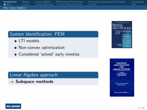
System Identification: PEM

LTI models

Non-convex optimization

Considered ’solved’ early nineties

Linear Algebra approach

⇒ Subspace methods

4 / 54


Why Linear Algebra?

Nonlinear regression, modelling and clustering

Most regression, modelling and clusteringproblems are nonlinear when formulated in theinput data space

This requires nonlinear nonconvex optimizationalgorithms

Linear Algebra approach

⇒ Least Squares Support Vector Machines

‘Kernel trick’ = projection of input data to ahigh-dimensional feature space

Regression, modelling, clustering problembecomes a large scale linear algebra problem (setof linear equations, eigenvalue problem)

5 / 54


Why Linear Algebra?

Nonlinear Polynomial Optimization

Polynomial object function + polynomial constraints

Non-convex

Computer Algebra, Homotopy methods, NumericalOptimization

Considered ’solved’ by mathematics community

Linear Algebra Approach

⇒ Linear Polynomial Algebra

6 / 54


Research on Three Levels

Conceptual/Geometric Level

Polynomial system solving is an eigenvalue problem in a large dimensionalspace!Row and Column Spaces: Ideal/Variety ↔ Row space/Kernel of M ,ranks and dimensions, nullspaces and orthogonalityGeometrical: intersection of subspaces, angles between subspaces,Grassmann’s theorem,. . .

Numerical Linear Algebra Level

Eigenvalue decompositions, SVDs,. . .Solving systems of equations (consistency, nb sols)QR decomposition and Gram-Schmidt algorithm

Numerical Algorithms Level

Modified Gram-Schmidt (numerical stability), GS ‘from back to front’Exploiting sparsity and Toeplitz structure (computational complexityO(n2) vs O(n3)), FFT-like computations and convolutions,. . .Power method to find smallest eigenvalue (= minimizer of polynomialoptimization problem)

7 / 54


Four instances of polynomial rooting problems

p(λ) = det(A− λI) = 0(x− 1)(x− 3)(x− 2) = 0

−(x− 2)(x− 3) = 0

x2 + 3y2 − 15 = 0

y − 3x3 − 2x2 + 13x− 2 = 0

minx,y

x2 + y2

s. t. y − x2 + 2x− 1 = 0

8 / 54


Outline

1 Introduction

2 History

3 Linear Algebra



6 Conclusions

9 / 54


Solving Polynomial Systems: a long and rich history. . .

Diophantus(c200-c284)Arithmetica

Al-Khwarizmi(c780-c850)

Zhu Shijie (c1260-c1320) JadeMirror of the Four Unknowns

Pierre de Fermat(c1601-1665)

Rene Descartes(1596-1650)

Isaac Newton(1643-1727)

GottfriedWilhelm Leibniz

(1646-1716)

10 / 54


. . . leading to “Algebraic Geometry”

Etienne Bezout(1730-1783)

Jean-VictorPoncelet

(1788-1867)

August FerdinandMobius (1790-1868)

Evariste Galois(1811-1832)

Arthur Cayley(1821-1895)

Leopold Kronecker(1823-1891)

Edmond Laguerre(1834-1886)

James JosephSylvester

(1814-1897)

Francis SowerbyMacaulay

(1862-1937)

David Hilbert(1862-1943)

11 / 54


So Far: Emphasis on Symbolic Methods

Computational Algebraic Geometry

Emphasis on symbolic manipulations

Computer algebra

Huge body of literature in Algebraic Geometry

Computational tools: Grobner Bases (next slide)

Wolfgang Grobner(1899-1980)

Bruno Buchberger

12 / 54


So Far: Emphasis on Symbolic Methods

Example: Grobner basis

Input system:

x2y + 4xy − 5y + 3 = 0

x2 + 4xy + 8y − 4x− 10 = 0

roots: (−1.7, 0.3), (0.5, 1.2), (6.0,−0.1), (−4.8, 2.9)

Generates simpler but equivalent system (same roots)

Symbolic eliminations and reductions

Depends on monomial ordering

Exponential complexity

Numerical issues! Coefficients become very large

Grobner Basis:

−9− 126y + 647y2 − 624y3 + 144y4 = 0

−1005 + 6109y − 6432y2 + 1584y3 + 228x = 0

13 / 54


Outline

1 Introduction

2 History

3 Linear Algebra



6 Conclusions

14 / 54


Homogeneous Linear Equations

Ap×q

Xq×(q−r)

= 0p×(q−r)

C(AT ) ⊥ C(X)

rank(A) = r

dimN(A) = q − r = rank(X)

A =[U1 U2

] [ S1 00 0

] [V T

1

V T2

]⇓

X = V2

James Joseph Sylvester

15 / 54


Homogeneous Linear Equations

Ap×q

Xq×(q−r)

= 0p×(q−r)

Reorder columns of A and partition

p×q

A =[p×(q−r) p×r

A1 A2

]rank(A2) = r (A2 full column rank)

Reorder rows of X and partition accordingly

[A1 A2

] [ q−rX1

X2

]q−r

r

= 0

rank(A2) = r

mrank(X1) = q − r

16 / 54


Dependent and Independent Variables

[A1 A2

] [ q−rX1

X2

]q−r

r

= 0

X1: independent variables

X2: dependent variables

X2 = −A2† A1 X1

A1 = −A2 X2 X1−1

Number of different ways of choosing r linearly independentcolumns out of q columns (upper bound):(

q

q − r

)=

q!

(q − r)! r!

17 / 54


Grassmann’s Dimension Theorem

Ap×q

Xq×(q−rA)

= 0p×(q−rA)

andBp×t

Yt×(t−rB)

= 0p×(t−rB)

What is the nullspace of [A B ]?

[A B ]

[q−rA t−rB ?

X 0 ?0 Y ?

]= 0

Let rank([A B ]) = rAB

(q − rA) + (t− rB)+? = (q + t)− rAB ⇒ ? = rA + rB − rAB

18 / 54


Grassmann’s Dimension Theorem

[A B ]

[ q−rA t−rB rA+rB−rAB

X 0 Z1

0 Y Z2

]= 0

Intersection between column space of A and B:

AZ1 = −BZ2

BA

rAB

rA

rA + rB − rAB

rB

#A #B#(A ∪B)

Hermann Grassmann

#(A∪B)=#A+ #B−#(A∩B)

19 / 54


Univariate Polynomials and Linear Algebra

Characteristic PolynomialThe eigenvalues of A are the roots of

p(λ) = det(A− λI) = 0

Companion MatrixSolving

q(x) = 7x3 − 2x2 − 5x+ 1 = 0

leads to 0 1 00 0 1

−1/7 5/7 2/7

1xx2

= x

1xx2

20 / 54



Consider the univariate equation

x3 + a1x2 + a2x+ a3 = 0,

having three distinct roots x1, x2 and x3

Write using Sylvester matrix as thesystem S ·K = 0:

a3 a2 a1 1 0 00 a3 a2 a1 1 00 0 a3 a2 a1 1

1 1 1x1 x2 x3

x21 x2

2 x23

x31 x3

2 x33

x41 x4

2 x43

x51 x5

2 x53

= 0

Homogeneouslinear system

RectangularVandermonde

corank = 3

Observabilitymatrix-like

Realizationtheory!

21 / 54



Shift property:1 1 1x1 x2 x3x21 x22 x23x31 x32 x33x41 x42 x43

[x1

x2x3

]=

x1 x2 x3x21 x22 x23x31 x32 x33x41 x42 x43x51 x52 x53

simplified:

K · I3 ·D = K · I3

This is a rectangular EVP with identity eigenvectors and roots aseigenvalues. For other basis Z with K = Z · T , we find

Z · T ·D = Z · T

So

calculate basis Z for null space

roots = eigenvalues D, T = eigenvectors22 / 54


Two Univariate Polynomials

Consider

x3 + a1x2 + a2x+ a3 = 0

x2 + b1x+ b2 = 0

Build the Sylvester Matrix:

1 a1 a2 a3 00 1 a1 a2 a31 b1 b2 0 00 1 b1 b2 00 0 1 b1 b2

1x

x2

x3

x4

= 0

Row Space Null SpaceIdeal=union of ideals=multiply rows with pow-ers of x

Variety=intersection of nullspaces

Corank of Sylvester matrix = number of common zeros

null space = intersection of null spaces of two Sylvestermatrices

common roots follow from realization theory in null space

notice ‘double’ Toeplitz-structure of Sylvester matrix

23 / 54



Sylvester ResultantConsider two polynomials f(x) and g(x):

f(x) = x3 − 6x2 + 11x− 6 = (x− 1)(x− 2)(x− 3)

g(x) = −x2 + 5x− 6 = −(x− 2)(x− 3)

Common roots iff S(f, g) = 0

S(f, g) = det

−6 11 −6 1 00 −6 11 −6 1

−6 5 −1 0 00 −6 5 −1 00 0 −6 5 −1

James Joseph Sylvester

24 / 54



The corank of the Sylvester matrix is 2!

Sylvester’s construction can be understood from

1 x x2 x3 x4

f(x) = 0 −6 11 −6 1 0x · f(x) = 0 −6 11 −6 1g(x) = 0 −6 5 −1x · g(x) = 0 −6 5 −1x2 · g(x) = 0 −6 5 −1

1 1x1 x2

x21 x2

2

x31 x3

2

x41 x4

2

= 0

where x1 = 2 and x2 = 3 are the common roots of f and g

25 / 54


Outline

1 Introduction

2 History

3 Linear Algebra



6 Conclusions

26 / 54


Null space based Root-finding

Consider{p(x, y) = x2 + 3y2 − 15 = 0q(x, y) = y − 3x3 − 2x2 + 13x− 2 = 0

Fix a monomial order, e.g. the degree negative lexordering: 1 < x < y < x2 < xy < y2 < x3 < x2y <. . .

Construct M : write the system in matrix-vectornotation:

1 x y x2 xy y2 x3 x2y xy2 y3

p(x, y) −15 1 3q(x, y) −2 13 1 −2 −3x · p(x, y) −15 1 3y · p(x, y) −15 1 3

27 / 54



{p(x, y) = x2 + 3y2 − 15 = 0q(x, y) = y − 3x3 − 2x2 + 13x− 2 = 0

Continue to enlarge the Macaulay matrix M :

it # form 1 x y x2 xy y2 x3 x2y xy2 y3 x4x3yx2y2xy3y4 x5x4yx3y2x2y3xy4y5→d = 3

p − 15 1 3xp − 15 1 3yp − 15 1 3q − 2 13 1 − 2 − 3

d = 4

x2p − 15 1 3xyp − 15 1 3

y2p − 15 1 3xq − 2 13 1 − 2 − 3yq − 2 13 1 − 2 − 3

d = 5

x3p − 15 1 3

x2yp − 15 1 3

xy2p − 15 1 3

y3p − 15 1 3

x2q − 2 13 1 − 2 − 3xyq − 2 13 1 − 2 − 3

y2q − 2 13 1 − 2 − 3

↓ ...

...

...

...

...

...

...

...

...

...

...

...

...

...

...

...

# rows grows faster than # cols ⇒ overdetermined system

rank deficient by construction!

28 / 54



Coefficient matrix M :

M =

[× × × × 0 0 00 × × × × 0 00 0 × × × × 00 0 0 × × × ×

]

Solutions generate vectors in kernel of M :

MK = 0

Number of solutions s follows fromcorank, provided M large enough (degreeof regularity, Hilbert function)

Multivariate Vandermondebasis for the null space:

1 1 . . . 1

x1 x2 . . . xs

y1 y2 . . . ys

x21 x2

2 . . . x2s

x1y1 x2y2 . . . xsys

y21 y2

2 . . . y2s

x31 x3

2 . . . x3s

x21y1 x2

2y2 . . . x2sys

x1y21 x2y2

2 . . . xsy2s

y31 y3

2 . . . y3s

x41 x4

2 . . . x44

x31y1 x3

2y2 . . . x3sys

x21y

21 x2

2y22 . . . x2

sy2s

x1y31 x2y3

2 . . . xsy3s

y41 y4

2 . . . y4s

......

......

29 / 54



Choose s linear independent rows in K

S1 K

This corresponds to finding lineardependent columns in M , going fromright to left over the columns

1 1 . . . 1

x1 x2 . . . xs

y1 y2 . . . ys

x21 x2

2 . . . x2s

x1y1 x2y2 . . . xsys

y21 y2

2 . . . y2s

x31 x3

2 . . . x3s

x21y1 x2

2y2 . . . x2sys

x1y21 x2y2

2 . . . xsy2s

y31 y3

2 . . . y3s

x41 x4

2 . . . x44

x31y1 x3

2y2 . . . x3sys

x21y

21 x2

2y22 . . . x2

sy2s

x1y31 x2y3

2 . . . xsy3s

y41 y4

2 . . . y4s

......

......

30 / 54



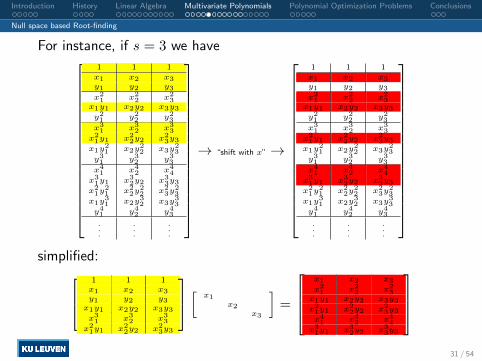
For instance, if s = 3 we have

1 1 1x1 x2 x3y1 y2 y3x21 x22 x23x1y1 x2y2 x3y3y21 y22 y23x31 x32 x33x21y1 x22y2 x23y3x1y

21 x2y

22 x3y

23

y31 y32 y33x41 x42 x44x31y1 x32y2 x33y3x21y

21 x22y

22 x23y

23

x1y31 x2y

32 x3y

33

y41 y42 y43...

.

.

.

.

.

.

→ “shift with x”→

1 1 1x1 x2 x3y1 y2 y3x21 x22 x23x1y1 x2y2 x3y3y21 y22 y23x31 x32 x33x21y1 x22y2 x23y3x1y

21 x2y

22 x3y

23

y31 y32 y33x41 x42 x44x31y1 x32y2 x33y3x21y

21 x22y

22 x23y

23

x1y31 x2y

32 x3y

33

y41 y42 y43...

.

.

.

.

.

.

simplified: 1 1 1

x1 x2 x3y1 y2 y3x1y1 x2y2 x3y3x31 x32 x33x21y1 x22y2 x23y3

[ x1x2

x3

]=

x1 x2 x3x21 x22 x23x1y1 x2y2 x3y3x21y1 x22y2 x23y3x41 x42 x44x31y1 x32y2 x33y3

31 / 54



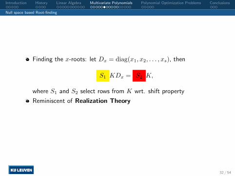
Finding the x-roots: let Dx = diag(x1, x2, . . . , xs), then

S1 KDx = S2 K,

where S1 and S2 select rows from K wrt. shift property

Reminiscent of Realization Theory

32 / 54



Nullspace of M

Find a basis for the nullspace of M using an SVD:

M =

× × × × 0 0 00 × × × × 0 00 0 × × × × 00 0 0 × × × ×

= [ X Y ][

Σ1 00 0

] [WT

ZT

]Hence,

MZ = 0

We haveS1KDx = S2K

However, K is not known, instead a basis Z is computed that satisfies

ZV = K

Which leads to(S2Z)V = (S1Z)V Dx

33 / 54



Possible to shift with y as well!

We then haveS1KDy = S3K

with Dy diagonal matrix of y-components of roots. This leads to

(S3Z)V = (S1Z)V Dy

Same eigenvectors V !

(S3Z)−1(S1Z) and (S2Z)

−1(S1Z) commute

34 / 54



Algorithm

1 Fix a monomial ordering scheme

2 Construct coefficient matrix M to sufficiently large dimensions

3 Compute basis for nullspace of M : corank s and Z

4 Find s linear independent rows in Z

5 Choose shift function, e.g., x

6 Solve the GEVP(S2Z)V = (S1Z)V Dx

S1 selects linear independent rows in Z; S2 the rows that are ‘hit’ bythe shift

(S1Z and S2Z can be rectangular as long as S1Z contains s linearindependent rows)

35 / 54



Modeling the null space: nD Realization Theory!

Illustrated for n = 2

Attasi model

v(k + 1, l) = Axv(k, l)v(k, l + 1) = Ayv(k, l)

Null space of Macaulay matrix: nD state sequence | | | | | | | | | |v00 v10 v01 v20 v11 v02 v30 v21 v12 v03

| | | | | | | | | |

T

=

| | | | | | |v00 Axv00 Ayv00 · · · A3

xv00 A2xAyv00 AxA

2yv00 A3

yv00

| | | | | | |

T

36 / 54



shift-invariance property, e.g., for y:−v00−−v10−−v01−−v20−−v11−−v02−

ATy =

−v01−−v11−−v02−−v21−−v12−−v03−

,

corresponding nD system realization


v(0, 0) = v00

choice of basis null space leads to different system realizations

eigenvalues of Ax and Ay invariant: x and y components of roots

37 / 54


Complications: Roots at Infinity

In general, there are 3 kinds of roots:

1 Roots in zero

2 Finite nonzero roots

3 Roots at infinity

Applying Grassmann’s Dimension theorem on the kernel allows towrite the following partitioning

[M1 M2]

[X1 0 X2

0 Y1 Y2

]= 0

X1 corresponds with the roots in zero (multiplicities included!)

Y1 corresponds with the roots at infinity (multiplicities included!)

[X2;Y2] corresponds with the finite nonzero roots (multiplicitiesincluded!)

38 / 54



Roots at infinity: univariate case

0x2 + x− 2 = 0

transform x→ 1X

⇒ X(1− 2X) = 0

1 affine root x = 2 (X = 12)

1 root at infinity x =∞ (X = 0)

Roots at infinity: multivariate case{(x− 2)y = 0

y − 3 = 0

transform x→ XT

, y → YT

⇒{

XY − 2Y T = 0Y − 3T = 0

1 affine root (x, y, T ) = (2, 3, 1) (T = 1)

1 root at infinity (x, y, T ) = (1, 0, 0) (T = 0)

39 / 54



Roots at Infinity: Mind the Gap!Dynamics in the null space of M for increasing degrees

nilpotency of action matrices of roots at infinity

corank stabilizes for 0-dim varieties

corank increases polynomially for positive-dim varieties (Hilbertpolynomial)

40 / 54



Weierstrass Canonical Formdecoupling affine and infinityroots (univariate)[

v(k + 1)w(k − 1)

]=[A 00 E

] [v(k)w(k)

]Singular nD Attasi model


w(k − 1, l) = Exw(k, l)w(k, l− 1) = Eyw(k, l)

with Ex and Ey nilpotentmatrices

Modeling the null space, e.g.,for n = 2, d = 4

v00 0v00Ax 0v00Ay 0v00A2

x w40E2x

v00AxAy w22ExEyv00A2

y w04E2y

v00A3x w40Ex

v00A2xAy w31Ex

v00AxA2y w13Ey

v00A3y w04Ey

v00A4x w40

v00A3xAy w31

v00A2xA

2y w22

v00A1xA

3y w13

v00A4y w04

41 / 54



Conclusion

Rooting multivariate polynomials

realization theory in the null space of the Macaulay matrixwith singular nD autonomous Attasi models

Number of affine roots and roots at infinity following fromdynamics of the mind-the-gap phenomenon. Two rankdecisions needed:

# roots (corank)# affine roots (column reduction)

Not treated here: multiplicity of roots

42 / 54


Outline

1 Introduction

2 History

3 Linear Algebra



6 Conclusions

43 / 54


Example Polynomial Optimization Problem

min x2 + y2

s. t. y − x2 + 2x− 1 = 0

Using Lagrange multipliers to find conditions for optimality:

L(x, y, z) = x2 + y2 + z(y − x2 + 2x− 1)

we have∂L/∂x = 0 → 2x− 2xz + 2z = 0∂L/∂y = 0 → 2y + z = 0∂L/∂z = 0 → y − x2 + 2x− 1 = 0

44 / 54


Everything remains polynomial!

System of polynomial equations

Finding minimizing root/solution: shift with objectivefunction! If AxV = xV and AyV = yV then

(A2x +A2

y)V = (x2 + y2)V

due to commutativity!

Polynomial optimization problems with a polynomial objective functionand polynomial constraints can always be written as eigenvalue problemswhere we search for the minimal eigenvalue!

→ ‘Linear Algebraization’ of polynomial optimization problems

45 / 54


System Identification: Prediction Error Methods

Polynomial Optimization Problems Applications

PEM System identification = EVP !!

Measured data {uk, yk}Nk=1

Model structure

yk = G(q)uk +H(q)ek

Output prediction

yk = H−1(q)G(q)uk + (1−H−1)yk

Model classes: ARX, ARMAX, OE, BJ

A(q)yk = B(q)/F (q)uk+C(q)/D(q)ek

H(q)

G(q)

e

u y

Class Polynomials

ARX A(q), B(q)

ARMAX A(q), B(q),C(q)

OE B(q), F (q)

BJ B(q), C(q),D(q), F (q)

46 / 54


System Identification: Prediction Error Methods

Minimize the prediction errors y − y, where

yk = H−1(q)G(q)uk + (1−H−1)yk,

subject to the model equations

Example

ARMAX identification: G(q) = B(q)/A(q) and H(q) = C(q)/A(q), whereA(q) = 1 + aq−1, B(q) = bq−1, C(q) = 1 + cq−1, N = 5

miny,a,b,c

(y1 − y1)2 + . . .+ (y5 − y5)

2

s. t. y5 − cy4 − bu4 − (c− a)y4 = 0,

y4 − cy3 − bu3 − (c− a)y3 = 0,

y3 − cy2 − bu2 − (c− a)y2 = 0,

y2 − cy1 − bu1 − (c− a)y1 = 0,

47 / 54


Structured Total Least Squares

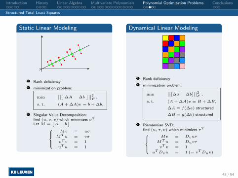
Static Linear Modeling

Rank deficiency

minimization problem:

min∣∣∣∣[ ∆A ∆b

]∣∣∣∣2F,

s. t. (A + ∆A)v = b + ∆b,

Singular Value Decomposition:find (u, σ, v) which minimizes σ2

Let M =[A b

]

Mv = uσ

MT u = vσ

vT v = 1

uT u = 1

Dynamical Linear Modeling

Rank deficiency

minimization problem:

min∣∣∣∣[∆a ∆b

]∣∣∣∣2F,

s. t. (A + ∆A)v = B + ∆B,

∆A = f(∆a) structured

∆B = g(∆b) structured

Riemannian SVD:find (u, τ, v) which minimizes τ2

Mv = Dvuτ

MT u = Duvτ

vT v = 1

uTDvu = 1 (= vTDuv)

48 / 54


Structured Total Least Squares

minv

τ2 = vTMTD−1v Mv

s. t. vT v = 1.

0 0.5 1 1.5 2 2.5 30

0.5

1

1.5

2

2.5

3

theta

phi

STLS Hankel cost function

TLS/SVD soln

STSL/RiSVD/invit steps

STLS/RiSVD/invit soln

STLS/RiSVD/EIG global min

STLS/RiSVD/EIG extrema

method TLS/SVD STLS inv. it. STLS eigv1 .8003 .4922 .8372v2 -.5479 -.7757 .3053v3 .2434 .3948 .4535

τ2 4.8438 3.0518 2.3822global solution? no no yes

49 / 54


And Many More Applications

Polynomial optimization problems

Matrix and tensor approximation problems

Affine, nonlinear and multi-eigenvalue EVP

Statistics

Weighted TLS. . .

Signal processing and System theory

PEMStructured TLSModel reductionIdentifiability of nonlinear model structures. . .

Computational biology

Conformation of moleculesMarkov modelling of DNA sequences. . .

. . .50 / 54


Outline

1 Introduction

2 History

3 Linear Algebra



6 Conclusions

51 / 54


Conclusions

Conclusions

Finding roots: linear algebra and realization theory!

Polynomial optimization: extremal eigenvalue problems

(Numerical) linear algebra/systems theory translation ofalgebraic geometry/symbolic algebra

These relations ‘linearly algebraize’ many problems

Linear algebraization: projecting up to higher dimensionalspace (difficult in low number of dimensions; ‘easy’ in highnumber of dimensions)

52 / 54


Conclusions

Open ProblemsMany challenges remain!

Efficient construction of the eigenvalue problem - exploitingsparseness and structure

Algorithms to find the minimizing solution directly (inversepower method?)

Unraveling structure at infinity (realization theory)

Positive dimensional solution set: parametrization eigenvalueproblem

nD version of Cayley-Hamilton theorem

reverse engineering: given zero set affine and at infinity, withmultiplicities. What is the set of multivariate polynomials ?

Analyzing and quantizing the (ill-)conditioning of the rootfinding problem

. . . 53 / 54


“At the end of the day,

the only thing we really understand,

is linear algebra”.

54 / 54

and Introduction: Professor Bart De Moor - Home pages of ESAT

Documents

Transcript of and Introduction: Professor Bart De Moor - Home pages of ESAT