7/

IA

EDGEWOOD ARSENAL CONTRACTOR REPORT(•) •_'•'c •t-CR,77028 .•

Report No. 10

hf) Final Teehnical Report

"ANALYSIS AND EVALUATION OFSUPPRESSIVE SHIELDS

by

P. A. Co- xP. S. Westine

CD J. J. Kulesz

L.LJ E. D. Espurza

c-.-

January 1978

SOUTHWEST RESEARCH INSTITUTEPost Office Drawer 28510, 6220 Culebra Road D D C

San Antonio, Texas 78284AF b. 19n,-R-ML MAAR 21 1978 I

Contract No. DAAA15-75-C-0083

I: J DEPARTMENT OF THE ARMY

Headquarters, Edgewood ArsenalAberdeen Proving Ground, Maryland 21010

Approved for public release) distribution unlimited.

', . .. . • •.•=• r,,•.,•,• , • .• • ._

*DIS"CLAI EINOTICE

\ ~C'

THIS ,DOCUMENT IS BESTQUALITY AVAILABLE. THE COPYFURNISHED TO DTIC CONTAINEDA SIGNIFWCANT NUMBER OFPAGES WHICH DO NOTREPRODUCE LEGIBLY.

REPRODUCED FROMBEST AVAILABLE COPY

Disclaimer

The findings in this report are not to be construed as an official Department of the Armyposition unless so designated by other authorized documents,

Disposition

Destroy this report when it is no longer needed. Do not return It to the originator.

I .oI. r

I - j I

( / ANALYSW AND.VALUAfIN OF THPISSV~IIED PAG (0976 -jun En977

An:AREPORT DCMETTINPAl BEOE~i~iih COM WN '& FAORMAbree roigGr oud Mayln 21010 ACCESSION NO -1I-i

IS. DITIB O STA w rcCME"HT (o41 Q'IRpo

Sin~~~Fia Techuraa reposePopllnrbrn,

fromLYIS JANuaryXIN FSPRSSV HE~s 1u 1976 thog June 197

S.PRO RMIN47 ~ORAIZTION NAM I NOV6 ADRES 10.T PROGRASSIFELEETD RJCTS2ccumry ~~ CLSP CýA 6O WORK ITh NUMBE RS~ Ot.BnwSoutwestReserch nsti~ute

SItLCU0MY CLA1SSM~CATION OF TH4IS PAGE(W7Ioti Dd~o Mata&d)

I SCCUgqgTY CLASSIFICATION OF YMIS PA09(fton Data Entered)

SUMMARY

This report documents work performed for the Edgewood Arsenal Suppressive Structuresprogram from January 1976 through June 1977. Included in this work was the developmcntof approximate energy solutions for the response of structures to blast loading, the analysisof strain data from the Category I 1/4-scale model tests, and calculation of pressure-timehistories for the burning of M 10 propellants in the Category V shield.

PREFACE

The investigation described in this report was authorized under PA, A4932, Project5751264. The work was performed at Southwest Research Institute under Contract DAAA 15-75-C-0083.

The use of trade names in this report does not constitute an official endorsement orapproval of the use of such commercial hardware or software. This report may not be citedfor purposes of advertisement.

The information in this document has been cleared for release to the general public.

"DDC

I~M2IWI6UhY~L~iLIT co ~' MAR 21 19T8

" ~~ ~~I ............... ... A I1T

DIT1I891l8IAVAIL. ITY COD/ L

[S U

3

TABLE OF CONTENTS

Page

1LIST OF ILLUSTRATIONS .................. ...................... 7

LIST OF TABLES ..................... .......................... 9

I. INTRODUCTION .................... ........................ 11

II. ADDITIONAL SOLUTIONS WITH ENERGY METHODS ..... ......... 11

A. Importance of the Assumed Deformed Shape .... ............ . .... I

1. Influence of Higher Modes ............ ................. 122. Influence of Other Shapes ......... ................. ... 17

B. Energy Solutions for Coupled Rigid-Plastic Systems ... ......... ... 19

1. Development of the Coupling Equation ..... ............ ... 202. Application to the Category I Shield .... ............. .... 213. Application to the Category III Shield ..... ............ ... 254. Importance of Treating Coupled Response .............. .... 30

C. Elastic-Plastic Energy Solutions for Beams ..... ............. ... 30

1. Solution for a Simply-Supported Beam .... ............ ... 312. String Solution ............. ..................... ... 323. Limiting Elastic and Plastic Cases ..... .............. ... 364. Approximate Elastic-Plastic Solutions .... ............. .... 38

D. Graphical Solutions for Beams ....... ................. .... 40

Ill. EQUATIONS FOR RESPONSE OF STRUCTURAL ELEMENTSTO BLAST LOADING ............. ..................... ... 50

IV. CATEGORY I 1/4-SCALE STRAIN DATA ANALYSIS ............. ... 55

A. Review and Summary of Experimental Data .................... 55B. Comparisons with Analytical Predictions ..... ............. ... 61

I . Predictions Using Approximate Energy Methods ............ ... 612. Predictions by Finite Element Methods .... ............ ... 65

C. Conclusions from the Strain Data Analysis . . . .......... 73

IL5 H________ _____ __________

TABLE OF COMTENTS (Cont'd)

Page

V. PRESSURES FROM BURNING PROPELLANT IN VENTED CHAMBEh; . . 73

A. Combustion Equations ........... .................... ... 73B. Gas Flow Equations ............ ..................... .... 74C. Effects of Burning Rates and Radiant Heat Loss .............. .... 76D. Comparison with Experimental Results ........... .............. 83

VI. DISCUSSION ................ .......................... .... 83

REFERENCES ................. ........................... .... 86

6

I.1 __________ ______

LIST OF ILLUSTRATIONS

Figure Page

I Rigid-Plastic Rheological Model . . . . ' . . . . . . . . . . . . 19

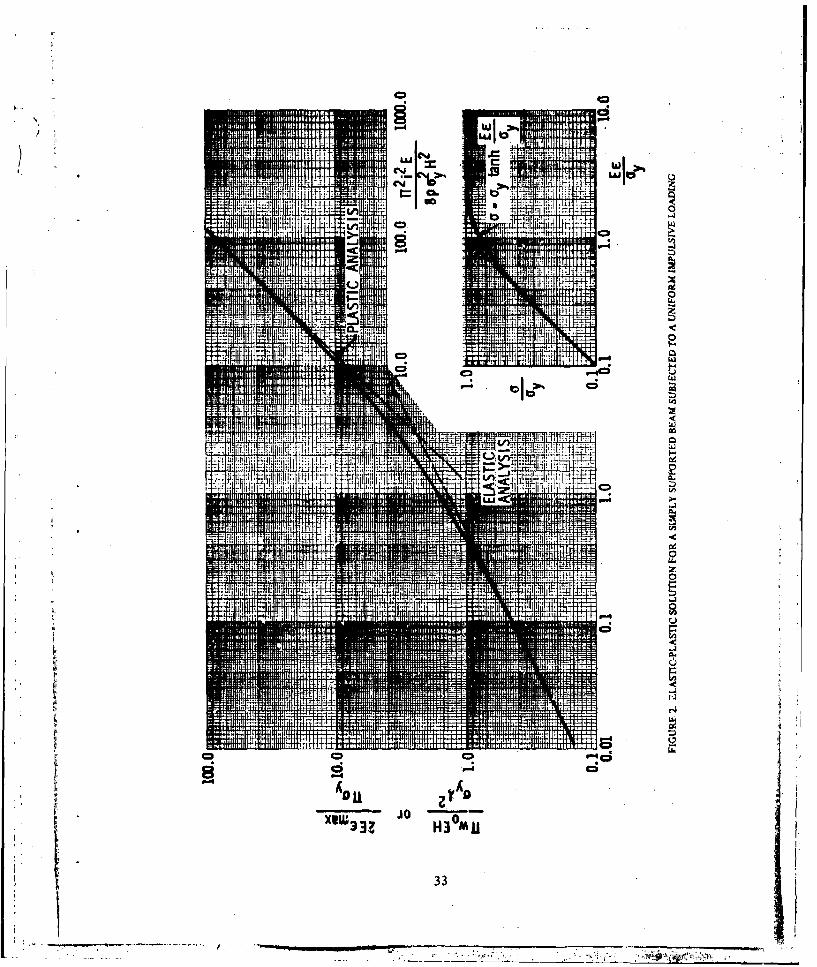
2 Elastic-Plastic Solution for a Simply-Supported Beam Subjected to aUniform Impulsive Loading ...... ....... ................... 33

3 Elastic-Plastic Solution for a String Loaded by a Uniform Impulse .... 35

4 Design Chart for Elastic-Plastic Beams Subjected to Initial Impulse

Plus a Quasi-Static Pressure ..... ............. ............ 46

5 Dimensions and Details of the Category I 1/4-Scale Model ......... ... 56

6 Strain Gage Locations on the Beams and Rings .... ....... .... 57

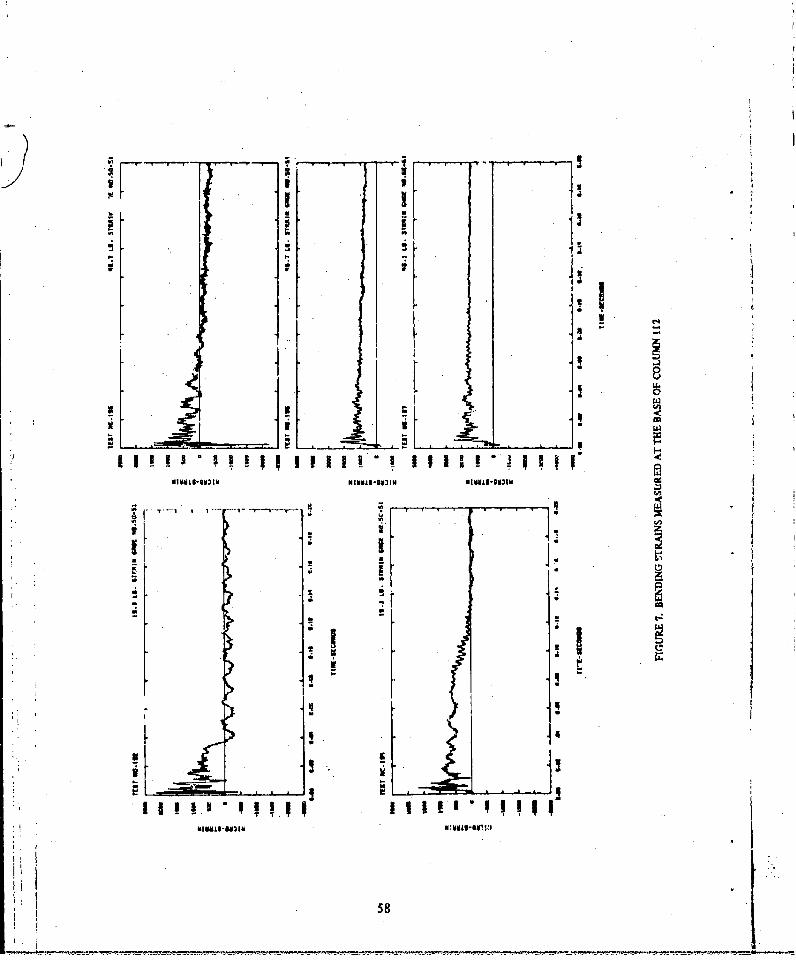
7 Bending Strains Measured at the Base of Column 112 ............ ... 58

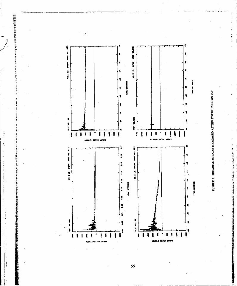
8 Shearing Strains Measured at the Top of Column 259 ............ ... 59

9 Schematic of the Finite Element Model of the Structure .. ....... .. 66

10 Distribution of Maximum Deflection, Strain and Shear Stress Values(9.3-lb charge) ......... ... ....................... .... 68

11 Distribution of Maximum Deflection, Strain and Shear Stress Values(45.7-lb charge) ......... ... ....................... .... 70

12 M 10 Propellant in Vented Chamber with no Radiation Loss .... ...... 79

13 MI0 Propellant in Vented Chamber with Radiation Loss .. ....... .. 82

7

LIST OF TABLESN

Table Page

I Impulsive Betnding Solution for a Simply-Supported Elastic Beam . 18

1I Impulsive Bending Solution for a Simply-Supported Plastic Beam .. 18

III Constants for Equation (141)) ......... .................. 45

IV Summary of Energy Solutions for Estimating the Deformation ofStructural Elements Subjected to Blast Loading ..... ........... 51

V Definition of Symbols Used in Table IV ..... .............. ... 54

VI Maximum Bending Strains Obtained from BRL Records ofCategor,, I 1/4-Scale Model Tests ....... ................ ... 60

VII Maximum Shear Strain Obtained from BRL Records ofCategory 11/4-Scale Model Tests ....... ................ ... 61

VIII Maximum Ring Strains Obtained from BRL Records ofCategory I 1/4-Scale Model Tests ....... ................ ... 61

IX Comparison of Peak Beam Bending Strains: Experiment toUncoupled Energy Solutions ........ .................. ... 63

X Comparison of Beam and Ring Strains: Experiment to

Coupled Energy Solutions ........ ................... ... 65

XI Beam Shear Data ......... ....................... ... 69

XII Measured and Calculated Strains in the Rings ...... ............ 71

XIII Comparison of Peak Values in the Beams ..... ............. ... 72

XIV M10 Propellant in Vented Chamber with No Radiation Loss .... ...... 80

XV M 10 Propellant in Vented Chamber with Radiation Loss .... ....... 81

9

ANALYSIS AND EVALUATION OF SUPPRESSIVE SHIELDS

I. INTRODUCTION

This final technical report documents work performed under Contract DAP.AI 5-75-C-0083for Edgewood Arsenal in support of the suppressive structures program. Principally, it includeswork performed during the time period of January 1976 through June 1977; however, someearlier work has been included in summary form. Also, some work performed during thistime period and documented in separate letter reports has not been included. Work performedprior to January 1976 is documented in References I through 9.

Contents of this report cover three different aspects of the work:

* The use of energy methods to predict deformations in olast-loaded structures,

* Strain data analysis for the Category I 1/4-scale model tests, and

* Calculation of pressure-time histories produced by burning propellant invented enclosures.

Chapter I1 contains recent work on the development of energy solutions for structuralresponse. This recent work includes a study of the influence of .tae deformed shape onthe accuracy of the solution obtained, energy solutions for coupled response, energy solu-tions for combined elastic-plastic behavior of beams and strings and the construction ofgeneral graphical solutions for blast-loaded beams. Chapter III contains a summary ofsolutions which have been developed over the total contract period.

Analysis of strain data from the Category I 1/4-scale model tests is covered in ChapterIV. Comparisons are made between measured strains and strains predicted by the approxi-mate energy methods and by finite-element methods. Chapter V describes the calculationprocedures and gives results for M 10 propellant burning in vented enclosures.

II. ADDITIONAL SOLUTIONS WITH ENERGY METHODS

A. Importance of the Assumed Deformed Shape

In using energy solutions to compute maximum deformations or strains in blast loadedstructural components, we select a deformed shape with appropriate boundary conditions.Usually, this assumed deformed shape is either the first mode from an infinite series of modes,or the static deformed shape carried over to a dynamic analysis. We will demonstrate thateither assumption can give excellent predictions of strains or deflections using either assumeddeformed shape. This generalization pertains for both elastic and plastic response of struc-tural components, and is true for both quasi-static and impulsive transient loads.

APAQX

1. Influence oj Higher Modes

A general deformed shape for a simply-supported elastic beam loaded with aunifurm quasi-static pulse ic given by Eq. (I).

cc N(1xy~)o F AN sin (1)

N= 1,3.5

The even modes are missing because of symmetry, and cosine contributions are missing be-cause of simply-supported boundary conditions. For bending only, the strain in the beam is

hdy r2 w2h , NAN sin - (2)

d ax'- 22 N-1,3,s

In a rectangular beam, t ..,e is given by:

U/2 Q/7Vol.=4b f dh f dx (3)

0 0

The strain energy U is:

U=, j 2 d V, (4a)

or:

U LrLEw.b1H/2 00 Q/2

Q4___ f h2dh N N4Akf sin" (,' Q (4b)0 N=1,3,5 0

The cross-products associated with squaring the strain integrate to zero in the precedingequation because of orthogonality of the mode shapes. Performing the rmquired doubleintegration gives for the strain energy:

00

U = !rEwI E bH3 AN (5)48 23

N= 1,3,5

Next we compute the maximurn possible wort. imparted to the structure with the deformedshape of Eq. (I). This work equals:

12

Q• 1 2 M i22 Nirx

wk = 2pbwv ,X AN f sin dx (6)

N = 1.3,5 0

Or, after integrating:

00

wk= 2pbw_ 2 ANir N()

N= 1,3,5

The Rayleigh-Ritz method can be used to obtain the relative amplitudes of the differentmodes. This is accomplished by subtracting the work from the strain energy,

00 0

(U -- wk) bH3 NA'4 A 2pbwQ , .k . AN (8)U482Q N Ir N

N = 1,3.5 N= t,3,5

and differentiating with respect to AN so the energy difference is minimized. This procedureyields:

a(U- wk) = ir4 EwobH3 N4Av 2pb~voA 1 = 0 (9)

6AN 24£3 7r N

or:

_48__ IAN ( i5-- o3') N- (10)

If one substitutes AN from Eq. (10) back into the preceding equations, a seriessolution for the deformed shape is obtained. The influence of higher modes can be obtainedby dividing AN by the amplitude of the first mode. This step yields

AN I(IA1 N 5

For a three-mode solution, the deformed sfiape will equal:

7r I 3irx I 70ýmwo ir. -+ -sin ---- +---sinn (12)

y w 243 2 3125

The paramctcr in equals 1.0038 if y is to equal wo at mid-span (at x/2 to 0.5). Substitutingfor in, differentiating Eq. (12) twice, and multiplying by --h gives the strain.

S7T 2Wh/I [ rx I 37rx 1 .5_rx_f - (.08 .... + •- sin • + • sin (13)

22 R027 k 12.5 R

13

-

From Eq. (4a),

t0- 120076 f h, dh f in nx: + 2sI 3nrx I irx\ =24) f ISh 2 dh J L sin -12- - sin--/ dx (14)

0 0

Performing the double integration gives for the strain energy:

( 1r4 Ebw,,oHlU= 1.053 ( 4-83 (15)

The factor 1.053 has been separated from the other terms in the precedir: .-quation,as this 5.3 percent increase in the strain energy U is the effect of adding the third and fifthmode contributions to the first mode estimate. A similar procedure will be followed inprest'nting the influence of high modes in subsequent relationships.

The work which must be equated to this strain energy is given by:

wk %2pb{I.OO38w) J sin +- - sin - + -- sin 5 dx (16)L £ 243 £ 3125

0

or, after integrating:

wk = 1.00524 E2DbwO j (17)

The influence of higher modes on the work is less than a 1 percent increase.Equating the work to the strain energy and solving for a nondimensionalized mid-spandeformation, w0 H/122 , yields:

woH1 r96pl21w--H= 0.9546 r96p3 (18)

This equation implies that the actual deformation will be less than that estimated with theone mode approximation, but the difference is less than 5 percent. The maximum strainscan also be estimated. Substituting 11/2 for h, Eq. (18) into Eq. (13), and 2/2 forx givesfor the maximum strain:

CmSX = 0.9304 (I9)

Equation (19) shows that the one mode approximation also overest"mates the strain in thisillustration, but that this error is lees than 7 percent.

14

We present one more illustration to show that these same conclusions can bereached for plastic as well as elastic response, and for extensional as well as bending behavior.As the second illustration, consider a string* with the deformed shape given by Eq. (1). Thestring has a different shape from a beam; however, this difference i5 reflected in the ANcoefficients. In a string,

d= ) 2 (20a)

or

00ff2' WO2

0 2 Nirx22 N 2 A'v cos 2 - (20b)

N= 1,3,5

The plastic strain energy equals the yield force times the strain integrated over the length:

•,v Q12'zr 2 F~~ 2/2 INirx\E N2A 2 f Cos2 - dx (21)N=1,3,5 0

or, after integrating:

U = N2A (22)42

N - 1,3,5

If the loading is a quasi-static pressure of intensity p, then the work is given by thepreviously obtained Eq. (7). We again use tne Rayleigh-Ritz method to obtain amplitudes ofthe different modes. Although our system is not conservative, it is linear because we havechosen to consider rigid-perfectly plastic mateiial behavior over the full range of deformation.Proceeding as before by taking the difference in the strain energy and work, we have

00 00

71`2F__W 2pbw0Q R - A_(U--wk) = , N 2Av w (23) I40 7r N

Nl - ,3,5 N 1,3,5

Differ -ntiating with respect to AN and setting the result equal to zero yields for AN:

,4 pb22 IAN = k7r3 Fy Wo A 3 (24)

*A string is defined here as an element with negligible bending stiffness.

15

A

Hence, the amplitude of various modes relative to the first one is

I A, N3 (25)

If we now proceed with a dynamic solution, the deformed shape for a three modesolution is given by:

y = mw, in 7Q + I7 sin 3r + I sin ] (26)

The parameter m equals 1.0299 because y is equal to w, at mid-span. Substituting intoEq. (20a) gives as an approximation for the strain:

1 7r I c W.'l Wx 1 31rx I 5_rx1 2C2-- 1.0 60 7 [os-+-•cos-- + - cos- (27)

[203 J I 2 9 R 25 2

The plastic strain energy is

W/2

U=2 f Fy c dx (28a)

0

or

jw/ 2 rx I 37rx I rx1U 1.0607 L 2 os-+- cos---I-cos dx (28b)

0

Performing the desired integration yields:

U= 1.2 2 -r-YJwO (29)

The work which must be equated to this strain energy is given by:

wk 2pb(.0299w)- sin - + sin dx (30)Q 27 R 125 Q0

or, after integrating,

wk- 1.0443[2pbw-- ] (31)

16

Equating the work to the strain energy and solving for a nondimensionalized mid-span defor-mation, w,,12, gives:

.08553 8 (32)

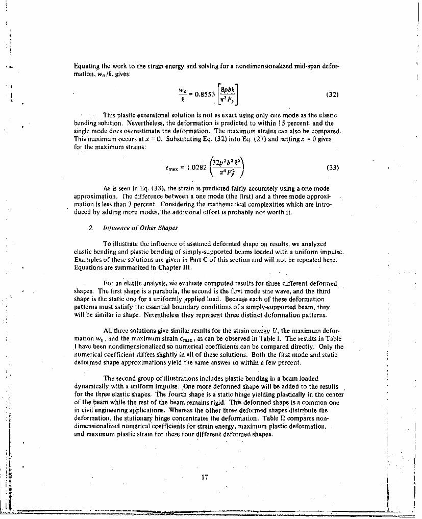
This plastic extensional solution is not as exact using only one mode as the elasticbending solution. Nevertheless, the deformation is predicted to within 1 5 percent, and thesingle mode does overestimate the deformation. The maximum strains can also be compared.This maximum occurs at x 0. Substituting Eq. (32) into Eq' (27) and nettingx 0 givesfor the maximum strains:

(32p•2 221Cmlx =,1.0282 2F7r-- / (33)

As is seen in Eq. (33), the strain is predicted fairly accurately using a one modeapproximation. rhe difference between a one mode (the first) and a three mode approxi-mation is less than 3 percent. Considering the mathematical complexities which are intro-duced by adding more modes, the additional effort is probably not worth it.

2. hifluence of Other Shapes

To illustrate the influence of assumed deformed shape on results, we analyzedelastic bending and plastic bending of simply-supported beams loaded with a uniform impulse.Examples of these solutions are given in Part C of this section and will not be repeated here.Equations are summarized in Chapter III.

For an elastic analysis, We evaluate computed results for three different deformedshapes. The first shape is a parabola, the second is the first mode sine wave, and the thirdshape is the static one for a uniformly applied load. Because each of these deformationpatterns must satisfy the essential boundary conditions of a simply-supported beam, theywill be similar in shape. Nevertheless they represent three distinct deformation patterns.

All three solutions give similar results for the strain energy U, the maximum defor-mation w0, and the maximum strain cmax, as can be observed in Table I. The results in TableI have been nondimensionalized so numerical coefficients can be compared directly. Only thenumerical coefficient differs slightly in'all of these solutions. Both the first mode and staticdeformed shape approximations yield the same answer to within a few percent.

The second group of illustrations includes plastic bending in a beam loadeddynamically w~th a uniform impulse. One more deformed shape will be added to the resultsfor the three elastic shapes. The fourth shape is a static hinge yielding plastically' in the centerof the beam while the rest of the beam remains rigid. This deformed shape is a common onein civil engineering applications, Whereas the other three deformed shapes distribute thedeformation, the stationary hinge concentrates the deformation. Table I1 compares non-dimensionalized numerical coefficients for strain energy, maximum plastic deformation,and maximum plastic strain for these four different deformed shapes.

17

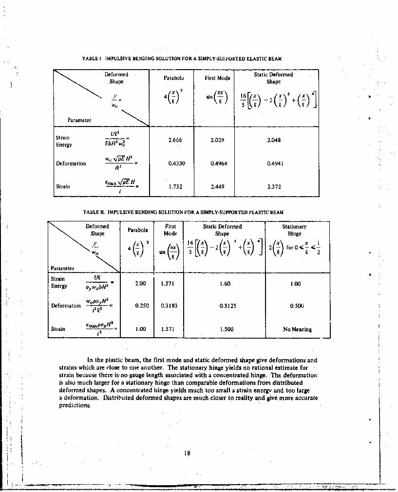
TABLE I IMPULSIVE BENDING SOLUTION FOR A SIMPLY-SUI'IOKTED ELASTIC BEAM

Deformed Parabola First Mode Static DeformedShape Shape

2 )2 sin(- 16

Parameter

SIrain u2Energy EbH3 we- 2.666 2.029 2.048

w,, vpTE H2Deformation - 0.4330 0.4964 0.4941

Strain efla Nx V/H 1.732 2.449 2.372i

TABLE i1. IMPULSIVE BENDING SOLUrION FOR A SIMPLY-SUPPORTED PLASTIC BEAM

Deformed First Static Deformed StationaryShape Mode Shape Hinge

(y4 x 16 -- 2 3+ 4 2 for•0 -S• 4sin Q \• 2

Parameter

Strain _ . _

Energy OywobH- 2.00 1.571 1.60 1.00

Deformation WoPOYtI 3 0.250 0.3183 0.3125 0.50O

Strain emaxPoy-f 1.00 1.571 1.500 No Meaning

In the plastic beam, the first mode and static deformed shape give deformations andstrains which are close to one another. The stationary hinge yields no rational estimate forstrain because there is~no gauge length associated with a concentrated hinge. The deformationis also much larger for a stationary hinge than comparable deformations from distributeddeformed shapes. A concentrated hinge yields much too small a strain energy and too largea deformation. Distributed deformed shapes are much closer to reality and give more accuratepredictions,

18

As these illustrations show, either a first mode approximation or.a static deformedshape is a good approximation. We would recommend a first mode approximation for sym-metric deformations. as in simply-supported and clamped-clamped beams, because the resultingalgebra is slightly easier. For nonsymmetric responses, as in a simply-supported clamped beam,the static del'ormed shape should be used. If the static deformed shape is not used in non-symmetric cases, uncertainty will otherwisc exist.

iolls In all of the illustrations, the assumed deformed shape being applied to a solutionis of less importance to the resulting deformations and strains than the effects of coupling.Supporting a flexible structural component oti a flexible foundation has a much greaterinfluence on structural response than the assumed deformed shape, as the next part of thissection shows

B. Energy Solutions for Coupled Rigid-Plastic Systems

In the suppressive structures program, energy solutions have been difficult to apply be-cause the actual structure is a combination of plates and beams or a combination of I-beamsand hoops, rather than a simple beam, plate. or membrane configuration. Although energysolutions developed to date in the Suppressive Structures Program (.see Refs. 1, 4, 6, and 9)apply for simple structural elements, structural configurations which are combinations ofelements canl also be solved using this approach; however, to complete such a solution, onemore equation is needed to couple deformation in the first structural element with defor-maltion in the second. For a rigid-plastic system, derivation of the required relationship isstraightforward.

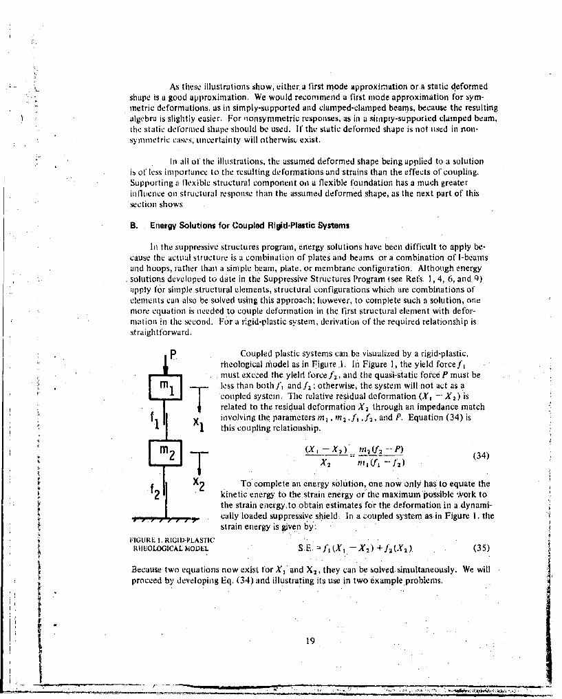
Coupled plastic systems can be visualized by a rigid-plastic,rheological miodel as in Figure .1. In Figure 1, the yield forcef Imust exceed the yield force f 2 , and tile quagi-static force P must beless than bothf', and f 2 : otherwise, the system will not act as acoupled system. The relative residual deformation (XI - X 2 ) isT related to the residual deformation X 2 through an impedance match

involving the parametersm 1m I, Pn2 .f, , f2 , and P. Equation (34) isthis coupling relationship.

m (XI-X 2 ) me2 (f2 -- P) (34)i [ ~X2 rn~l(i' -J`]2 )(4

VX To complete aan energy sohition, one now only has to equate the2 kinetic energy to thestrain energy or the maximum possible work to

the strain energy to obtain estimates for the deformation in a dynami-cally loaded suppressive shield. In a coupled system as in Figure 1, thestrain energy is given by:

FIGURE 1. RIGID-PLASTICR1IEOLOGICAL NODEL . S.E =fl (XI -X 2 ) + f 2 (X) (35)

Because two equations now exist for X, and X2, they can be.solved.simultaneously. We willproceed by developing Eq. (34) and illustrating its use in two exampleproblenms.

19

1. Developrnent of the Coupling Equation

Assume m I is hit simultaneously with an impulse I and a quasi-static force P. Thenthe two equations of motion are:*

m1 - 1 +fj =P (36a)

tn3.2 +f2 4' 1 (36b)

For no initial displacement, no initial velocity for m2 , and an initial velocity of 1/mr for in,we obtain by direct integration:

It f, r2 Pt 2

x =- - +- (37a)mI 2rn1 2m,

(f, -- f2 )t2

x-4 = (37b)2M2

Coupled motion continues until (x - x2) equals zero,

dx2 O r f +(38))t -)( + 2 m 2 mI

or until time t' given by

V = 2 (39)[m + m2 )f 1 -- mnf 2 7-m 2 PJ

At this time, the new initial conditions for m2 are:

,m 2(f, - ()0aXA2

2 [(ml +rma)f, -= m-f -- mP] 2. (40a)

dx-- (f--f 2 ) (40b)di [(mI + m 2 )f, --mlf2 --m 2 P]

The relative motion (x - x2) equals the maximum relative residual motion (XI - X 2 )

(XI - X2 ) "2(41)2n I[(mI + m 2 )f1 -- M f2 -m 2 P]

After element f, "locks up" at time t' motion continues as an uncoupled system.The equation of motion in this'second phase is given by:

*Note that I is total Impulse with dimenslons of FT, rather than poctfle blast impulne I with dimensions of FT/L'.

* 20

______________

(inm + m 2 ):2 +f 2 P (42)

By establishing a new time zero at the instant I* when the motion becomes uncoupled, usingthe initial conditions given by Eqs. (40), and integrating, we obtain as the equation for dis-placement in the second phase:

-(1'2 - P)t2 (V1 - 1' Y)t M_ 2_ Q-1 1 )PX2 = + +1 (43)201n + 'n2) 2 (pitI + i2)f' - in 1'21 2[(in + in 2 )f Y- 1 2 ]2

All motion stops at time It given by:

It (in I + i m2 )(f, - f2)1V(2 -P)mmI +m 2 )fl -mfJ'2 -m 2 P]

Substituting It into Eq. (43) and gathering terms gives the maximum residual deformation,X2, for element m2.

(f, -f 2 )12 (42(f- -P)[(mI + m2 )fl -m f 2 -m 2P] (45)

Finally, dividing Eq. (41) by Eq, (45) gives the relative displacement coupling equationalready presented as Eq. (34).

(XI -X 2 ) m2 (V2 - P) (34)X-2 mI V, - f2 )

This equation is the key coupling relationship which will be used in all calculations. Use ofthe equation is best illustrated by some example problems. Calculation of the mass m for astructural component is no problem; however, the effective force f requires assumptions whencalculated for a beam or plate element. We will calculate the forcef by assuming a deformed

* shape for a structural component, calculating the strain energy stored in that deformed shape,determining the average deformation for a given deformed shape, and finally dividing thestrain energy by the average deformation. Once this procedure is complete, the couplingEq. (34) and energy relationships permit structural deformations and strains to be deter-mined in a procedure similar to that used in any uncoupled structural analysis.

2. Application to the Category I Shield

The Category I shield is used as the approximate illustrative example because it.was the first to draw our attention to the need for a coupled solution. Here we will derivethe equations for coupled response of the beams and iings. In Chapter IV, comparisonswith data from the Category I 1/4-scale model demonstrate the validity of the coupledenergy solution.

Basically, this shield is a barrel as shown in Figure 5 (page 52). External circularhoops provide restraint for longitudinal I-beams. The I-beams represent the mi - f1 structure,and the hoops are the inm - fa structure. We will treat the I-beams as clamped-clampedbeams. An assumed deformation pattern for this structural component is given by:

21

we( WO +o. 27r) (46)where

we = maximum mid-span deformation relative to the supports

2 = total span

x = coordinate system with origin at mid-span

y -- deformation at some value of x

Differentiating Eq. (46) twice gives:

dzy -27r 2 wo 21rx-" 2 Cos (47)

The strain Energy S.E. 0 i6 given by the integral

Q/2 d2 yS.E. = 2 f MY- dx (48)

0

where

My= plastic yield moment

Substituting Eq. (47) into Eq. (48) and completing the desired integration gives:

S.E.( -- (49)

The average deformation YAVG must be calculated next. It is obtained by the integral

IlkYAvG•2 f - I + Cos ,x (50)0

oroWO

YAVG = 2- (51)2

The force fl in one beam equals S.E. 0 divided by the average deformation, or:

f= (52)

22

22I

The mass mi equals:

in, =PbAbR (53)

where

p, = mass density of a beam

A b = cross-sectional area of a beam

NextJ'2 and m2 must be calculated for the hoops. if we assume hoops of equaleffective cross-sectional area, Ah, on each end, the deformation will be a symmetric changein radius AR. The strain energy for both hoops is:

S.=E. (2Oy) R (27rRAh) (54a)

or

S.E.q) = 47wyAhAR (54b)

The average deflection in a hoop is the deflection AR. This means that the force f 2 is givenby:

f2 = S.E.a /AR (55a)

or

fo2 41royA h (55b)

The mass m2 equals twice the mass density times the area times the circumference, or:

m = (2ph)(A, )(2rR) (56a)

or

m 2 41rphAhR (56b)

The quasi-static force P equals the pressure p times the internal circumference times thelength, or:

P = (p)(27rr)(Q) (57a)

p = 21rrkp (57b)

Now the coupling equation can be used to relate the average deformation in thebeams (wo/2) to the deformation in the hoops AR. Substituting form,, m 2 ,f, ,f ,andP then yields:

• 23

IVo

2 = (4wrphAhR)l(41rOhAh )- 21rr] (58)AR (N-) 47r(hA8)

The parameter N stands for the number of beams. The mass of the beams and force equalsN times m I or.f' , respectively, for a single beam in Eq. (58). In addition, the yield stressob times the plastic section modulus z was substituted for the yield moment in the beamforce equation. Eq. (52). Reducing Eq. (58) algebraically gives the ratio for the maximumdeformation in the beams relative to the change in hoop radius.

8rphAhR I prkWo NPbAb2ohAh (59)

AR [2 ( N~bZ

1

\OhAhR)--1

The solution proceeds by writing the strain energy S.E. for the entire system.This energy equals the sum of Eqs. (49) and (54), or:

S.E. = 41rNabZWo + 4rohAh AR (60)

Substituting Eq. (59) for AR in Eq. (60) gives:

4lrNcrbzw 0 NpbAboh•Wo [2 ( Nubz .S.E. - +__ _ L OhAhk) (61)

2 2phR (I prA,2ahAh

Next the energy imparted to the structure must be estimated. This energy comesfrom the kinetic energy imparted through blast waves and the work from the quasi-staticpressure buildup within a suppressive shield. Algebraically, this energy EN equals Eq. (62)with loads imparted to the beams.

NI2

EN,= +Pb2(YAVG + AR) (62)

where

b loaded width of the beams.

Substituting for 1, ml , YAVG, and Eq. (59) for AR yields, after collecting terms:

24

____ [ 2NObZNM2 b 2q+ pbQw 0 NpbAbk \ahAh (63)EN + - 11.O+ ' rQ• (632pbAb 2 47rphAhR R \2Ih J

Finally, equating EN, Eq. (63), to S.E., Eq. (61), and gathering terms yields an equationwhich can be solved for w0, the maximum deflection in the beams.

_2b_+___ pb02 + NpbAb9 \ahA)s - = I) OhPbAbQ' 2ohAh

+ .+ . (• r-_/ 8+ )iprpbAbuhZW 0 N 4vphAhR I pr ObphzR I prk\ 2uhAhlJ 2u,,A h)

(64)Equation (64) yields w0 , the maximum beam deformation relative to the rings,

and subsequent substitution in Fq. (59) yields AR, the change in hoop radius. Strains canalso be estimated. The residual hoop strain equals ARIR as in Eq. (65a), and the maximtmresidual bending strain in the beams equals half the beam depth H12 times the maximum beamcurvature as given by Eq. (47). Equation (65b) is the maximum reseidual strain in the beams.

ehoup R (65a)R

C rmw0s Q2 (65b)

Refer to Chapter IV for calculations based on these equations for the l]4-rcale model of theCategory I shield.

3. Application to the Category III Shield

The second example will be that of a rectangular membrane, supported rigidlyalong two opposite edges and by flexible clamped-clamped beams along the other twoedges. This configuration might be representative of the original Category III containmentstructure" 9) which was replaced by the 1/4-scale Category I shield. We begin by assuminga deformed shape for the membrane, Eq. (66).

w;ý WO Cos 7XCos 7Y(62X 2Y (66)

In a membrane the strains are calculated from the first derivatives of the slope by:

I {aw\ 2 7(2W0EXX = \ -8 sin cos2 (67a)

25

................... .... .-... '....,....

Im = 2 8r2 7Y 2 2 27/

,.y ý:( = W) - (!') sin 2n(sin(67b)

In a structure under a biaxial state of stress, the strain energy per unit volunte is given bythe integral:

S-o =f_ ox dexx + 2 axy de.y + ayy dEyyJ (68)

If we assume a rigid-plastic material with a yield point in the plate ap, then oxx = Uyy = upand u.Y = ap/l/3 according to the distortion energy yield theory. Substitution of constantstresses into Eq. (68), integrating Eq. (68) for strains, substituting the strains from Eqs. (67)into Eq. (68), and expressing the volume of the membrane through the thickness times adouble integral yields:

X Y rS E.0 4 f dx f dy sin' cos 2

0 0

+2-ph-Tw2 sin (-J sin (r)- (69r2w)V/i 16XY•" 8Y2

X cos2 r sin 2 (h;)'Performing the required double integration gives:

S =r2aphwo [Y 1.6 +X (70)S .E'. " 8 Lx +/,•

The average plate deformation must be calculated next by double integration.

x Y( 4 XY)WAVG = 4 f dx f dy w, cos 2X 2Y (71)

o 0

or:

WAVG 4 (72)

I2

26

1 ~~~~~~~~~~. ... . . . ..... .. . v..... . • ." -. - -... -- w., , .

The force f' in a plate equals S.E.() divided by wAVG, Or:

47r' ohw[Y 16 + 1X32 -J (73)

The mass in equals:

min = 4pphXY (74)

Next,f 2 and m2 must be calculated; however, this has already been done in thefirst example. Because there are two beams, the quantity f2 equals twice fin Eq. (52), andthe mass m 2 equals twice in in Eq. (53). These results are summaiized as Eqs. (75).

f/2 =6M Y (75a)2

m., 2PbAQ (75b)

The average deflection of the beams is still wb /2, and the quasi-static force is given by Eq. (76).

P = 4pXY (76)

We are now prepared to substitute into Eq. (34). Substituting for m, m2JI, f 2 , and Pyields the coupling equation for deflections.

8wp_ =327prPM0,A - 8PbPXYAQ (77)

2it2 Wb pj X jiophw, Y + 16 -+X 161rMl 77S4p~hXYL2 J

or:

7rP~u~h2XYwI 164 X 6p

32 pbmA - -X + 72 PbAk)(78)

4M,

The solution proceeds by writing the strain energy S.E. for the entire system. This energy istwo times Eq. (49) for the strain energy in one beam plus E-I. (70).

87= Wb+r2o(,ph wP2Y 16 XS.E. M + +- [(79)

S8

27

S~27

i -

Substituting Eq. (78) for wb and collecting terms yields:

S.E. W2 up hva 1 2p X Yh __Y 16 XSE 8 (1 pY\ X + -_"ý +

L b2 4M (80)

S128pp,MyX'hwp

irPbAQ2 (I pXY4

The kinetic energy from the blast wave which is imparted to the system equals:

t2 (4XY) 2 2W2 XY2(4ppX]h) pph

The work from the quasi-static pressure loading equals:

WK = p(4XY) W( + "wb) (82)

Or after substituting Eq. (78) for wb:

[ 8 I• rp[Y 16

WK= 2p.YwP V2 2 +32PbM A (IP 4y)

L PXY-](83).

16pphXY 1SpXYA7 2 PbAR I( PX-Y. ]

Equating WK + KE to S.E. gives the final solution. In nondimensional format this solutionis:

"± ~ 0.3927i1rp~,,wrr2w 6'484vrprw= 0.6169lr, + 7rp [0.8106,7. + "-066L_ (4 -wrw,,p) (4 -- 7rp)jS~(84a)

SX i +- 8-r I iry4'--81.48( 4 -- r.7rp)J ir,,(4 - 7r.','o)

where

rp -•X YhTP (84b)

28

iI

fOR

PRX Y

SP XY (84b)(Concl)

Y 16 XiTy - + + Zr

7tw W-

h

Equation (84) is a quadratic equation that must be solved for 7r, or wp. After wp is ob-tained, ivb is obtained from Eq. (78), wh.'ch in nondimensional format is:

%vb 0.3927r5 7r, 7y7rw - 6.484wr(4), _•v. ... •(85)WP (4 -- 7r. 7rp

To comolete this illustration, let us apply Eqs. (84) and (85) to the Category Illshield. We will assume parameters as follows:

p 66 psi

1 0. 179 psi-sec

X 26.5 in.

SY 56.5 in.

h 1.033 in. (this is an effective thickness)

lb-sec2

Pp Pb =7.33x 10- in. 4

a = ob =48,000 psi

A = 61.71 in.'

S= 113 in.

My = 1.21 X 10+'7 in.-lb

S. 29

fF

Substitution of these parameters into the fr terms gives:

1T'0 = 0.2218

7r, = 0.4783

ir, = 1.929

=r1 1.197

try -= 3.537

Substituting into Eq. (84) gives a positive root for 7r, of 3.953; hence, wp 4.083 inches.Finally, 3ubstitution into Eq. (85) gives Wb = -1.135 inches. This negative sign associatedwith wb is not a mistake. It means that the plate and beam systems are not coupled as hasbeen assumed; hence, this analysis is not appropriate for the parameters substituted into it.In this particula. sclution. f2 is greater than fl. This means there is no plastic deformationin the second element, and the particular sy-tcmn under investigation is uncoupled. Appro-priate answers can be obtained by using uncoupled techniques which have already beenpreseiuted. The purpose of this second iliustration was to emphasize the meaning of anegative sign when it is encountered in this type of analysis.

4. Importance of Treating Coupled Response

We have shown that eneigy solutions are possible for coupled perfectly plasticsystems. For two members in a codpled system, one additional equation is needed to relatedeflections in the first member to deflections in the second member. Equation (34) ispresented as a relationship for coupling the deflections. With the assistance of this oneextrz equation, energy solutions can be developed as in any rigid-plastic coupled system.

In Chapter IV we will show that the effect of coupling is very important for pre-dicting respoase in the Category I shield. On the other hand, the example above showsthat coupling is unimportant for predicting membrane deformations in the Category IIIshield. While these solutions are more complicated than uncoupled solutions, residualdeflections and strains for coupled systems can be predicted with cloed-form algebraicsolutions, and the usefulness of the approximate energy methods for predicting responseto blast or impact loading is greatly enhanced.

C. Elastic-Plastic Energy Solutions for Beams

In the design of suppressive shields we are usually interested in predicting onset offailure, and hence maximum strain or maximum strets. In most problems, a beam hassegments which remain elastic and segments which go plastic. The assumptions of totalelasticity or total plasticity throughout a!l elements in a structural component, or concen-trated plasticity in a hinge, are approximations. To obtain an idea of how elastic-plasticsolutions could be presented to designers, and to see how combined solutions might beobtained from simple elastic and/or simple plastic solutions, two elastic-plastic solutionshave been developed for a simply-supported beam and a string.

30

• The constitutive relationship used for boih solutions is given by Eq. (86).

Ecoa=y tanh (86)

oy

This is an excellent approximation to an elastic-plastic material. For small strains, Ee/oy <0.5. the stress-strain curve is a linear one with a EEc and, for large strains, Ee/ay. > 2.0,the stress-strain curve is a perfectly plastic one, with a oy.

L. Solution for a Simply-Supported Beam

In any structural element under a uniaxial state of stress, the strain energy perunit volume is given by:

U = fade (87)Vol.

If we substitute Eq. t86) for a and integrate from a strain of zero to the maximum strain e,we obtain:

Vol. f y tanh de (88)0

Or:

UU = n cosh (89)Vol. E LOY/

Equation (89) is then applied to any bending or extensional solution by substituting thestrain and integrating over the volume. If we use the assumed deformed shape for a simply-supported beam given by the first term of Eq. (1), the strain e for a differentivl element inbending is:

S3.

e=w-hd = h sin- (90)x2 22

If the beam is of rectangular cross sectioni, the volume equals:

•H2 Q12

SVol. = 4b dh dx (91)0 0

Substituting the expression for e and the volume integral into Eq. (89) gives the followingdouble integration for the strain energy U... . -

42bH12 2/2 rw h wrb cosh W E On dh dx (92)

311.1

or

w12 " /3 , r/"- H E (93a)•. E f f k. coh ,o sin/ do dot

0 0

where

o =xx/R and 13 h/H. (93b)

Next we assume that the loading is a uniformly applied impulse, giving for the kineticenergy:

P1 2 bPHKE .. (94)

2m 2pH

Equating the kinetic energy to the strain energy and rearranging yields the dimensionlessequation:

(.K " 2. 12 WL2 \ro " n.Y H2y f f ). ooh %•r- in a]dO du (95)

': "0 0

This equation can be written as:

Pr/2 2 DC= f f R cosh Dflsin d doa (96a)

where

C =(i 212E/gpc•hf) and D (,rwoHE/oay 2 ) (96b)

A computer program was required to numerically perform the double integration. Resultsof this program are represented by the solid continuous line in Figure 2. Dashed lines inthe figure are the asymptotes for completely elastic or fully plastic behavior. Note that theelastic-plastic solution correctly approaches the elastic asymptote for small deformationsand the plastic asymptote for large deformations.

2. String Solution

The string solution uses the same strain energy per unit volume equation, Eq. (89),as the beam solution, These solutions differ in the equations relating strain to deformation.In an extensional element the strain Is given by Eq. (20a). Substituting the first term ofEq. (1) for the assumed deform.ed shape in Eq. (20a) gives Eq. (97).

2J 2£-- - - c o 2 O x(9 7 )

32

II

_i ,..~ ~,~--

If-49 FMOIT M0

C~U,

fill J IP. CL

soa

'd V0

INIF

C CD

011 1 L

.I1 . I 3J .O .N3 .... ... : . TM1

...................................!l

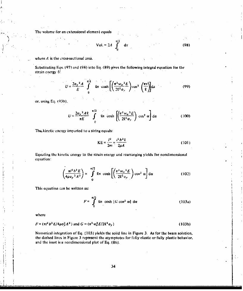
The volume for an extensional element equals

Vol.'2A f dv (98)0

where A is the cross-sectional area.

Substituting Eqs. (97) and (98) into Eq. (89) gives the following integral equation for thestrain energy U.

U = _• z..._ f 9"1 C•O Ol - Wo' ON' 2 ('os d X¢ (99)f f .Los 22 o~/.0 lj. d

or. using Eq. 493b),

U: 2AQ f/ n cosh FCos 2 da (100)u E7 - LK 221ao /

The.kinetic energy imparted to a string equals:

12 i 2b 2 (0

2m 2pA

Equating the kinetic energy to the strain energy and rearranging yields the nondimensionalequation:

2 f (n coSh\ -cos2 da (002)(4pux2 A2J i055 1 [ )2o~0

This equation can be written as:

F= Vf ii cosh IG cos2 a] da (103a)

where

F(i 2 b2 E/4p.A 2 ) and G (r 2 woE/222 Ov) (103b)

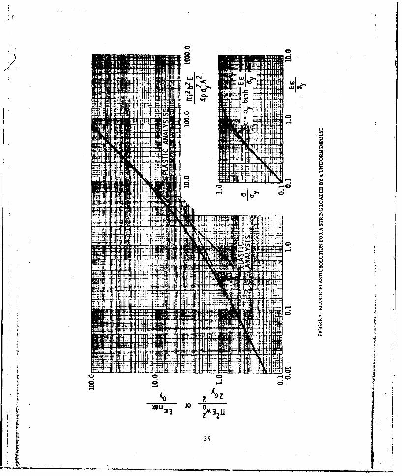
Numerical integration of Eq. (103) yields the solid line in Figure 3. As for the beam solution,the dashed lines in Figure 3 represent the asymptotes for fully elastic or fully plastic behavior,and the inset is a nondimensional plot of Eq. (86).

V3I

CC

HWU _4

A0L I m, C, J w1.1 .

UU

It ~ ~ ~ ~ ~ ~ ' 6,tllill ,5 I

.7-ag IW §P

I_ I i U!I;

Although the elastic-plastic solutions given in Figures 2 and 3 are extremely usefulfor designers. they are somewhat difficult to derive because numerical integration is required.We will now show that the numerical solution can be approximated to within one or two per-cent by properly combining the elastic and plastic asymptotes. The asymptotes are easilyderived.

3. Limiting Elastic and Plastic Cases

Before an approximate elastic-plastic solution can be found, the asymptotes arerequired. Although these limiting cases have been derived many times before (see Refs. I.4, 6. and 9), we will rederive them here for completeness.

In elastic problems, the strain energy per unit volume, Eq. (87) becomes:

U_ E 2 (104)Vol. 2

In plastic problems, the strain energy per unit volume, Eq. (87) becomes:

Vol.= aye (105)

Of course, these equations apply to either the beam or string solution.

For the beam solution, both elastic and plastic strains are given by Eq. (90),and the volume equals the double integial given by Eq. (91). Substituting these two equationsinto Eq. (104) for the elastic case or Eq. (1 05) for the plastic case givel:

elastic:

H1/2 /1227r 4 EWo 2 b /•

Q4 f f h2 sin 2 dhdx

0 0

rigid-plastic:

2 H1 /2 R/2

U f f h sinT d dx (107)0 0

Or, after completing the required double integration-:

elastic:

M =r 4 Ewo bH3- 48 (108)

36

rigid-plastic:

U W2 (109)2k

Now, by equating Eq. (108) to Eq. (94) and Eq. (109) to Eq. (94). the elastic and plasticasymptotes, respectively, of Figure 2 are obtained. These are given by Eqs. (110) and (I I I).

(elastic beam)

1224 if4

pEw02 H4 24 (110)

and

(rigid-plastic beani)

pay woH2

For the string solution, both elastic and plastic strains are given by Eq. (97), andthe volume is given by the integral in Eq. (98). Substituting these two equations into Eq.(104) for the elastic string or Eq. (105) for the plastic string gives:

elastic:

,U= n 4 f cos4 !x-dx (112)

rigid-plastic:

r 2f2 oW0 2 A (•7irxX d

L 2- f cos2 (113)2 2

0

Or, after completing the required integrations:

elastic:

~37r4 EA wo 43 wU (114)

64R3

37

rigid-plastic:

U 73'VY . 2(115)4k

The elastic and plastic asymptotes for the string solution are obtained by equating Eqs. (114)and (115), respectively, to the kinetic energy given by Eq. (101). Equations (116) and (117)obtained in this way are the asymptotes of Figure 3.

(elastic string)

i2b2 j 4 37(4

pEA2wo 4 32 (116)

and

(rigid-plas~tic string)

i2b~2k2 7r (17

puoA 2 wo 2 2 (117)

The approximate elastic-plastic solutions can now be derived.

4 Approximate Elastic-Plastic Solutions

The elastic-plastic solutions in Figures 2 and 3 are very closely approximated byEq. (118) where Y is the ordinate, X is the abscissa, and coefficients A and B are constants.

Y =A tanh2 (BX)' /2 (118)

The elastic asymptote for Eq. (118) is:

(elastic asymptote)

Y-X (AB) (I119a)X

And the plastic asymptote is:

(plastic asymptote)

Y= (A) (I 19b)

These equations have the same form as the asymptotes for the beam and the string. Thus,for the simply supported beam the terms in Eqs. (119) are defined by comparison withEqs. (110) and (I0 ). We tind:

38

-*--.---------ll -------, ------ . ---.- *. I==== .,,( =-_ L.:: %• •.".• lllll~• • • •gllll I~rlll~l •1Illl ~ lo ••-

12 £2

po•wYH" (120a)/ pay w H02

X pEw0 2Hf (120b)

A 7ir (120c)

AB 7 4 (120d)24

Solving for X and B and substituting into Eq. (118) gives an accurate approximation to theelastic-plastic bending solution without encountering the inconvenience of a numericalintegration of a complicated function.

i 2k2 =[3.1416 tanh2 1.1366 ( o )• . 2 (121)

To compare with Figure 2, this solution can be recast in the format:

1r Y 1 F~~,H (rw H 12H--- w1.234 L tanh 0.641 (2 ,a)

8ay 2 H [ R 2

or

SC~ 1.234 D tanh2 (0.641 D' 2 ) (122b)

Either of the preceeding formats is acceptable for the elastic-plastic beam solution.

The advantage to the format given by Eq. (1 22) is that the deformation w0 is isolated on oneside rather than appearing on both sides. Designers would prefer to isolate w, in this mannerbecause this deformation also directly deternines the maximum. strain. Equation (122) is notthe computed line appearing in Figure 2; however, it is very difficult to detect differences inEq. (122) and the computer solution.

Equation (118) and its asymptotes can also be used to obtain an accurate approxi-mation to the string solution. The elastic and plastic string solutiont are given by Eqs. (116)and (117). Comparing Eqs. (119) to these equations, we have:

Y P b2 R2 02a

X PEAZw04 (123a)

Q2Y Pa b2 R

!Y=po•,,A~wo 2 (123b)

(123b)324I AB = 32 (1 23c)

. 39

A (123d)N 2

Solving for B and X and substituting into Eq. (118) yields:

2 2 [tanh 2.356 WyL0, ] (124)payA w0

2 2 (Y 2'1

Or after modifying the format to isolate tet:ms containing w, on one side and using Eq. (I 03b),

r Ari2 Eb 2 1 . 785 Ew, 2 2 ( 2 I/S=0.7854 tanh2 0612.4 7r Ew1025a)L~1pay 2AJ La Ru~2 J 0 [ 'R'

or

F= 0.7854 G tanh2 (0.6124 G" 2 ) (125b)

This solution also approximates the more detailed elastic-plastic solution with thesame degree of accuracy as the bending beam analysis. Philosophically, one should not bedisturbed by the use of the hyperbolic tangent squared as a function for combining elasticand plastic solutions. After all, any solution requires an approximate stress-strain curve.No approximation to a stress-strain curve uniformly matches all materials. Instead ofapproximating the stress-strain curve, one can elect to approximate the strain energy trans-ition from elastic to plastic as we have done.

D. Graphical Solutions for Beams

The procedures developed in the precedirng section can be used to derive general graphica!solutions for blast loaded structural elements. These graphs are attractive because they permitrapid solutions to difficult problems without recourse to complicated mathematical procedures.In fact, as we will demonstrate, the graphical solutions are self-contained and can be easilyapplied.

Our example for these solutions will be beams loaded in the same manner as those inthe case of the Category I shield. These beams are subjected to an initial impulse producedby the shock wave, plus a long duration quasi-static pressure produced principally by the

* heating of air in a confined space. Because the blast wave part of the loading is described* only by an initial impulse (not a pressure and impulse or pressure and time), this solution is

suitable only when the duration of the overpressure in the blast wave is less than one-quarterof the fundamental period ot the beams. The pressure, p, in this solution refers to the quasi-static pressure, not the blast wave overpressure.

In response to these loads, the beams undergo elastic and plastic deformations. Forthis example, coupling between the beams and rings is neglected, but different end conditions,i.e., simply-supported, clarIped or a combination of the two, are included.

40

The solution to this problem is similar to the impulsively-loaded beam solved in SectionC except that an additional term is required to define the energy produced by the action ofthe quasi-static pressure. p. on the beam as it displaces. With the addition of this term calledthe work. WK. the energy balance is written as

KE + WK -- U (126)

KE is the kinetic energy produced by the initial impulse, and U is the strain energy (elasticand plastic) stored or absorbed by the beam.

Kinetic energy is the same for each beam regardless of the support condition and isgiven by Eq. (94), derived previously. The work and kinetic energy depend upon the modeshapes assumed, and this will differ for each support condition. For these calculations, wehave assumed that the deformed shape under dynamic loading is the same as the staticdeformed shape. The calculations are illustrated in detail for a simply-supported beam.

The static deformed shape for a uniformly-loaded, simply-supported beam is giveil byEq. (127)

y =16w (X4 - 29x 3 + R3x) (127)

where w0 is the center deflection (x = 2/2). We can now derive the work from the quasi-static pressure p as

WK= pby dx (128)

where b is the beam loaded width and Q is its length. Substituting Eq. (127) into (128) and* performing the required integration, the work is foand to be

16WK = pb2wo (129)

As shown in Eq. (90), the strain in a beam cross-section at a distance h above or belowthe neutral axis is

d2 ye -h (130)

Again using the deformed shape of Eq. (127), we have

16w,e -h (-i2X - 12U) (131)

41

The strain energy can now be computed from Eq. (89); however, the solution can be made moregeneral if we reformulate the strain energy in terms of gross cross section properties of thebeam. This can be don- by replacing the stress-strain constitutive relationship given in Eq. (86)by an approximalion for the moment-curvature relationship. Such a relationship is given byEq. (132)

E/y"M MP tanh M (132)Mr,

where j " is the second derivative of the beam displacement with respect to x (curvature), andAl, is the fully plastic moment of the beams. Notice that Eq. (132) has exactly the form ofEq. ,82). It was not derived from Eq. (82) and represents a slightly different approximationto the stress-strain behavior. In fact, the stress-strain behavior will differ slightly for beamsof different cross-sections.

The strain energy per unit length for a teain in bending can be written as

U /Ely" 4f2 /Elyf (133)- f MP, tanh - d~v"~ P- n cosh I

Fcr the tctal strain energy, Eq. (133) is integrated over the beam length, R, to obtain:

M VU E f ncosh (v C-) d (134)

Substituting for y" from Eq. (127) gives

Vu-j ' R coh[/iv 19 (X2 - X) d (135)"I f 5

It is convenient to nondimensionalize the integral by letting

t •- dx R d/t (136)

With these substitutions wo have

I -

U=M-- f En cosh E .v0 192 Z2 d' (37)El K q, 5)S0

42

Now substituting Eqs. (94), (129), and (137) into Eq. (126), we obtain Eq. (138). whichrelates the deformation of a simply-supported bean! to its basic properties and the blastloading parameters;

_2 ~ ncoh .) 19IQ• 1":'PO£ +2p 516 pb~w° EM Vnes t-• --- ll- dt (138)

2pA 25 OElf [PR 50

Equation (138) is nondimensionalized by dividing each side by the coefficient of the integral,or:

12 b2El 16pbElw0 f Elwo 1+ c) E( ) dt (139)2M2 A 25M2 J 5f cos

In nondimensional pi terms, the equation is:

/ 192\1rI +r 2 =7 f n cosh 3 Q(2--1) d( (140)

0

A more convenient relationship is obtained if w. is eliminated from all but one group. Thisis accomplished by rewriting ir2 as the product of 7r3 and a new group 7r,,.

ff 2 = (16pb22 7r' f'E-w (141)

AAlso, if one wishes to limit the maximum strain in the beam rather than the mrximnumdeformation, w, can be replaced by fmax in 7r3 uring Eq. (13 1). For a simply-supportedbeam, emax occurs at x = Q/2 and h H/2. Thus,

Miv,

24era 5 (142)

With this sub3tituticn, 7r3 becomes.

* _5EIemax7r3 - (143)

!. ~2041pt H

* INow Eq. (139) becomes:

f !l•m+ S en cosh2 Mp~/r?4)kaPMP) kieMPh) f 1( L4ph)

(144)

"43 "

where the constants in 7r6 and T3 have been replaced by cvp and a, respectively.

Similar equations car, also be derived for clamped-clamped and clamped-simply-supportedbeams. If we again use the static deformed shape under uniforta loading, the followingequations are obtained.

Deformed Shape

c-c: y= Ž W(x4 - 2k2x + Ox")

7.7w, x 3 1cIss:- y = - V'-X - + -232 2

Strain Equation

Oc." C = -h--2-- (6X2 -6Ux + Q2)

7.7wo _c-as." e.= -h--- -- (2x• 9£R)

Maximum Strain

i 6Hwoc-c: eM~y _Q

11 .55HwoC$S." emax = -

J 2

The defo;med s1~apes are substituted into Eq. (128) to compute the work, and the strainexpressions are substituted into Eq. (134) to compute the strain energy. These expressionsare then combined with the kinetic-energy (Eq. (94)] according to Eq. (126) to obtain ex-pressions similar to Eq. (138). Performing the manipulations described for simply-supportedbeams and generalizing the results, an equation can be obtained which applies to all threeboundary conditions. It is given by Eq. (145).

2 + (pbR 2 Efem.,X cosh rE~~\P VrP74 kCrm ctMjxMPH [cz-.MH

* 0 (145)

X (Ct' + C2t+ C3 ) dt

Note thlnt the only difference between Eqs. (145) and (144) is in the descripton of thenondimensional deformed shape. The proper equation for each beam boundary conditionis obtained by substitution of the appropriate constants am defined in Table Ill;

44

__1

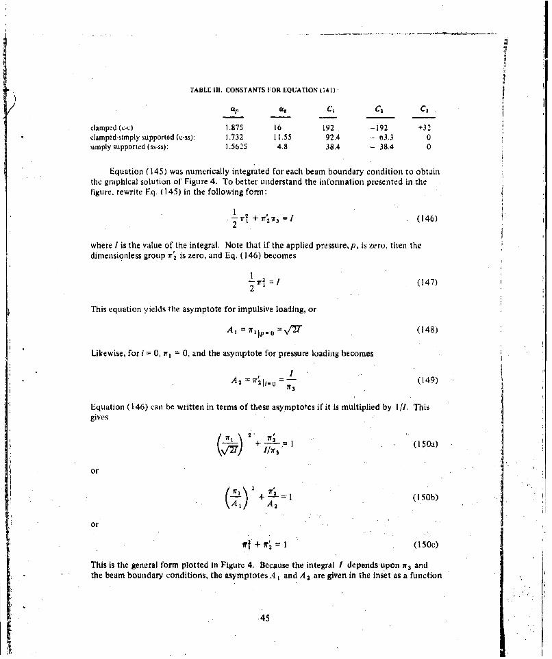
TABLE Ill, CONSTANTS FOR EQUATION (141)

11, C, C3 C3

clamped (c-c) 1.875 16 192 -192 +32clamped5slmply supported (c.ss): 1.732 11,55 92.4 -- 63.3 0simply supported (ss-ss): 1.5625 4.8 38.4 - 38.4 0

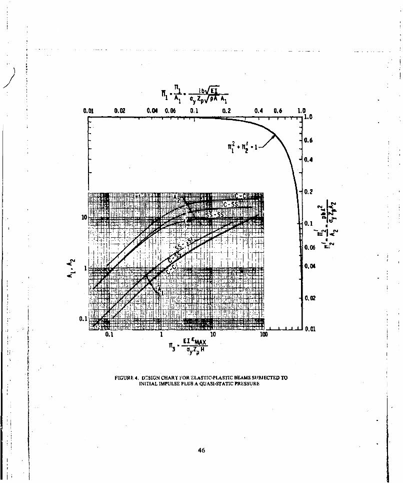
Equation (145) was numerically integrated for each beam boundary condition to obtainthe graphical solution of Figure 4. To better understand the information presented in thefigure, rewrite Eq. (145) in the following form:

2 rt + r 2•7r 3 =I (146)

where I is tile value of the integral. Note that if the applied pressure, p, is zero, then thedimensionless group ?r' 2 is zero, and Eq. (146) becomes

-Wj =I (147)2

This equation yields the asymptote for impulsive loading, or

A p.0 =ir0 V"2"T (148)

Likewise, for 1 = 0, 7r, 0, and the asymptote for pressure loading becomes

IA 2 =' =- (149)

Equation (146) can be written in terms of these asymptotes if it is multiplied by 11l. Thisgives

+ =1 + (150a)

or

-A + r+2 (150b)

or

1r2 + f =I(1S5c0

This is the general form plotted in Figure 4. Because the integral I dependsupon ir3 andthe beam boundary conditions, the asymptotes A I and A 2 are given in the Inset as a function

.45

1 A1I c azp /VrP Al00 0.2 0.04 0.06 01 0.2 0.4 0.6 1.0

0.01 0.021.0

120.

0.4

0.2

10.

0.04

.7-9 0.06

0.01

TI V

3 ayZIIH

FIGURE 4. D:SIGN CHART FOR ELASTIC-PLASTIC BEAMS SUBJECTED TOINITIAL IMPULSE PLUS A QUASI-STATIC PRESSURE

46

of 7r., and the beam boundary conditions. One difference in the graphical solution and theform given by Eq. (145) is the absence of the constants cup and a. Because separate curvesare plotted for the different boundary conditions, these constants could be eliminated. Forexample, to eliminate ip, the 7r2 asymptote, A 2, was simply multiplied by the constantgiven for (k, in Table Ill for the appropriate boundary condition.

Observe that the solution for either impulsive loading only or for pressure loading only isgiven directly. This is clear from Eq. (150b) and from Figure 4. Ifp 0, for example, then7r3 0 and we have

A, 7r, =m (151)

Thus, if the beam properties and the impulse are known, A can be computed and -t3 readdirectly from the appropriate curve in Figure 4. Alternately, if one wished to know whatimpulse would produce a prescribed strain in a beam, 7r 3 could be evaluated, A 1 read fromthe graph, and I computed from Eq. (15 1).

A similar approach holds for pressure loading only; however, for the case of an initialimpulse plus a quasi-static pressure, an iterative approach is required. Consider as an examplethe beams in the cage of the Category I 1/4-scale model. Beam properties and the loadingparameters are listed below. (Refer also to Chapter IV.)

Beam Properties: Loading:

A = 1.67 in.2 1 0.48 psi-secI= 2.52 in.4 p 190psi

z= 1.95 in. 3

b = 143 in. (loaded width)H '3.0 in.£ 30 in.

Soa 45,000 psiE= 30 X 0psip = 0.000733 lb-se 2 /in. 4

With these values, 7r, and 7r2 can be computed.

it 1 =-~~--1.944

7r. 2 2.787'

To find the maximum strain in the beams, first conmputý the values for pressure and impulseseparately.

Impulse only: A1 I r = 1.944

47

From Figure 4 for a clamped (c-c) beam:

3 =Iemax 2

Emx 0.01114

Pressure only: A,2 7ra2 2.787

From Figure 4,

EIemax13- - 0.235

emx = 0.000818

The beam is more sensitive to the impulse than the pressure. Also, the maximum strain forthe combined loading will be larger than the sum of the strains computed separately. There-fore, try

Em1x 1.l(0.01114 + 0.000818) 0.01196

For.this strain, 7r3 is:

r13 3.434

and from Figure 4,

A, = 2.02 A2 17.9

A, and A 2 must satisfy Eq. (1 50b) (or the curve in Figure 4), which for this problem becomes

1.944 2 + 2.787

Substituting Al and A 2 gives

(i1.944)2 (1.71) .8- - .9 1.082

For a closer result, try

1.944A, 0.995 = 2.1

48

C ! 4

From Figure 4, the corresponding values of A 2 and 'r are

A 2 = 18.1

7r3 3.65

Now check Eq. (1 50b) again.

S2.787

2.1 18.1

This result is close enough. Therefore, the maximum strain for the S3 X 5.7 beams in the zCategory I 1/4-scale model for clamped ends and rigid support is predicted to be

= 3.65 ' 0.01271 = 12 ,7 10OgeEl

Also note that, with the asymptotes A/ and A, deteimined, the entire p-i diagram, for a* maximum strain of 12,7 1Ope in the beam, can be established from Eq. (150b) o, from Fig-

ure 4. So, what we have really obtained is a general solution for the, beam at, not just thesolution for one set of loading parameters.

"If one wishes to compute maximum deflection in the beams, the relationship betweenmaximum strain and the deflection can be used. For a simply-supported beam, this relation-ship is given by Eq. (142), and, for the other boundary conditions, by the expressions onpage 44. Generaizing, we can write

W= (152)

where ae is given in Table Ill,

Thus, we have obtained a general graphical solution which includes: A

* beams of different boundary conditions (with rigid support)

* elastic-plastic beam behavior .1

# predictions of maximum strains and deflections

0 beam response predictions for any combination of an initial impulse, 1, afdquasi-static pressure, p.

Such a solution provides a convenient tool for preliminary design of beams subjected to thisparticular type of loading. For final design, a more rigorous approach is usually required,which includes the effects of support flexibility, etc. The need for a more rigorous analysiswill be demonstrated by the comparisons in Chapter IV between measured and predictedstrains for thf- Category I 1/4-scale model.

49

Ill. EQUATIONS FOR RESPONSE OF STRUCTURALELEMENTS TO BLAST LOADING

Numerous equations for estimating the response of structural components to blastloading have been developed during the Suppressive Structures Program. Derivations ofthese equations have been reported by Baker, et al].(') by Westine and Baker,( 6 ) and byWestine and Cox.A4) A partial summary was included in the report by Baker, et al."9 )Here, a final summary is made which collects the equations reported in References 1,4,and 6, plus othei equations that have not previously been reported, Equations presentedare for the response of individual structural elements. Rigid behavior of the componentwhich loads the element or the support for the element is assumed. Equations for coupledresponae have been developed for a few cases, but these are included separately in ChapterII. Chapter I1 also includes graphical solutions for selected components

This summary, given in Table IV, is an expansion of Table B-I in Reference 9. Cor-rections to equations have been made, as required, and both elastic, elastic-plastic and rigid-plastic solutions are included. Structural elements covered include beams, rings, membranes,plates, cylinders, and spheres.

Equations in Table IV relate the peak deformation in the structurai element, usuallydesigroted as w0 , to the element's material and geometric properties and to the applied loading.The applied loading is treated as the simultaneous application of an impulse, ir, and a quasi-static pressure, p. This loading is representative of that on suppressive structures producedby the internal detonation of a high explosive. The blast wave from the detonation is ofshort duration relative to structural frequencies (and so can be treated as an impulse), andheating of the air in the structure produces a pressure buildup of much longer duration.Simultaneous application of the impulse and quasi-static pressure is supported by pressuremeasurement from the 1 / 16.scale venting tests reported by Schumacher and Ewing( I ) a:ndby pressure data from the Category I 1/4-scale model tests reported by Schumacher, et al."I 2)

For purposes of deriving the equations, the quasi-static pressure is assumed to be a step loading(zero rise time) to a constant value. If either ir or p is zero, the equations reduce to the properpressure or impulsive asymptote, respectively.

Each equation is based upon an assumed shape for the final deformed state of the struc-tural elements. The deformation patterns used are given in the table. For some elements,solutions are given for more than one deformed shape. This is true for a beam with clamped

ends which experiences bending deformations only. The first solution used a parabola as thedeformed shape, and the second solution uses a higher order polynomial. Deformations pre-dicted by the first equation compare favorably to experiment(t ); however, bending strainsin the beam associated with a parabolic deformed shape are constant. The second equationhas net been compared to expeiiment, bvt the strain distributions produced by the deformedshapes are more representative of true beam behavior. A third solution is also given whicil is

based upon the siatic deformed shape. Notice that the constants in the equations derived forthe polynomial and for the static deformed shape differ only slightly.

Parameters which enter the equations in Table IV are defined in Table V. Also, thegeometry of the element is sketched in Table IV for additional clarification. because theequations are nondimensional in their present form, any consistent set of units is permissible.

50

iii

i. .•- - '_ _ - -

"i"ilt

-- ! •.cc

IrvCA~ Kn c

Nil7

i~jj jI~i ii

II I51

P q I S. .

VIP

0 JILiOZ to.•;

I i52

52

N

I

o II-i�i : II"

�I h�j �

'I. ii-- - 3.

� I-

it I'I III

U j

V � :j�p�I; � IiI' 4 II

iI�f II p I

I.

53

*LJ

TARLE V. DFFINITION OF SYMBOLS USED IN TABLE IV

Symbol Definition

A beam cross-sectional area

AR ring cross-sectional nrea

b loaded width of beam

CSBR circumferential beam spacing in the I-beam cylinder measured at RR

E material elastic modulus

h thickness of plate, or shell

ir specific reflected impulse from Initial blast wave, plus reflectionsif applicable

L length of beam for which the deformation is being determined;length of cylinder

LI, loaded length of the cylinder supported by a single ring

ma mass per unit area of any additional material (non load bearing)which is attached to the sphere or dome

MT total mass supported by a ring (includes the ring mass)

Mp beam plastic moment

N factor in the beam equation; N = I for simple support, N = 2 forclamped support

p quasi-static pressure

SPy axial yield force of the heam

r radius to arbitrary point on a circular plate

R mean radius of a sphere or cylinder, radius of a circular plate

RL loaded radius in the cylindrical shield

RR mean radius of the ring

AR radial expansion of the ring, dome, or cylinderw lateral deflection of a beam or plate at point x, or r, respectively

WO center deflection of a beam or plate

x distance along the beam or plate, normally measured from the center

X short semi-span of the plate

y distance along plate center line normally measured from the plate center

Y long semi-span of the plate

p material density

oy yield strength of the material

v Poisson's ratio

54

IV. CATEGORY I 1/4-SCALE STRAIN DATA ANALYSISN

Measurements of strain in the beams, rings, foundation, aad roof of the Category IlI4-scale model were made. by Schumacher, et al.."' 2) in tests conducted at the BRL.6 Model dimension. and strain gage locations are shown in Figures 5 and 6. Structuraldetails are given in the Corps of Engineers' drawing No. 6003, "Suppressive Shield, QuarterScale Model, Category I." One of the principal objectives of the tests was to determine thestructural adequacy of the shield and to evaluate the analytical methods used to supportthe shield design.

SwRI was assigned the task of analyzing strain data recorded on the beams and rings.Data were provided by BRL in the form of computer-generated plots. The plots were re-viewed and peak strains were extracted from records which appeared to be consistent fromtest to test and with gages at similar locations. These peak values were then comparedwith analytical predictions. The comparisons allowed us to draw some conclusions aboutthe strains and analysis methods which are covered at the end of this chapter.

A. Review and Summary of Experimental Data

A brief description of each test conducted on the model is given below. All chargeswere spherical Pentolite, centrally located. Closure strips and liners referred to in the testdescriptions are shown in Figure 5.

Test 191: 8.3-lb charge- 1/4-scale model without closure strips or liner

Test 192: Same as Test 191, but with a charge of 19.3 lb

Test 193. 19.3-lb charge-closure strips added to cover the spaces between everysecond pair of inside beams

Test 194: 19.3-lb charge--all spaces between the inside beams covered with closurestrips

Test 195: 45.7-lb charge-same configuration as for Test 194 except that additionalweld bead was added along the sides of the closure strips, and shims wereadded to eliminate free travel by the beam before contact with the ringwas made.

Test 196: 45.7-lb charge-weld repairs were made and a 24-gage corrugated steelliner was added inside the closure strips to seal the shield.

Test 197: 45.1-lb charge-ring repairs were made, and two 22-gage corrugated steelliners were added inside the closure strips to seal the shield.

We limited our comparisons between analysis and experiment to those tests with allclosure strips installed. Thus, comparisons were made with data from Tests 194 through197 and include comparisons for both the 19.3-lb and 45.7-lb charge weights.

Figures 7 and 8 are typical of the strain plots received from BRL. Bending strains atthe base of column II 2 (see Figure 6) are given in Figure 7 for Test 192 and Tests 194

55

Ring

Outer Beam

4-in. Reb--r Studr, on 6-.In. Center

Spacers Located Clocure Stripat the Rings

ILiner

KMENF--rBem -

A -A1* 10oft

I I

Zi ft(typ)

i I AI I

-131 ft

FIGURE 5. DIMENSIONS AND DETAILS OF THE

I •

I I

CAT R I 1 L M

i t '" __ l56

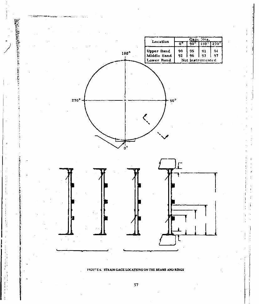
S• ~~~~~Location 0I tO gO

Upper Band 90 95 91 94

Middle Band 9Z 96 93 97

Lower Band Not instrumentyd

Z70 0 go0

%

_ .1

FI .

LJ

gT

S,_ _ _ _ _ _ _

i I_

FIUE6. sTRAIN GAGE LOAIN ON THE BEAMSO AND RINGS i

IIr

-'- - SP

I I I UI.,

- U U UU I .1

* S U* U U

;I I 80

S

IUIEISUII 33 33333.3 3333313Uk3* I-.RU SUDS U 5 33UM!�E�13

NIUNz3-OU3�w u:wu�s*ev�Iai'd2

-I.-'. -

- S 4

I IS zI�. U I.a 1:

Ut U

IU

U - q -

-� L q- U

I

-5ILL��

liii ! I ! I � 111111 I 1: *1M1VNLI-4Ij1�4

58

� -

9 � -, -r-rir q

I II ¶

I III

IV I r I

IiI* I I-

- p

8

I I*1

MIiniUAU�IN N3U0 uIWVU-fl�Iii IiW3I4S

St- j-,------�----mr�� - I

I - I U

I -

k II.

* a U -�

U U U

*

-I

U II

I5 3 I

IuIII!�I!IIuIWhL-Q�IU hW�46 NIVU�SOM�tN U�3

59

through 197. The effect of progressive scaling of the shield is apparent from the reduceddecay rates. The character of Test 195 is noticeably different from the others because it

) decays sooner than expected and has a negative value late in time. Shims were inserted be-tween the beams and the rings before this test, and the change in response character can beattributed to the change in support. Figure 8 gives the history of the principal strain com-puted from rosette No. 85, which is located at the top of column 259. From these records

it appears that slight yielding in shear occurred even in the early tests. Reasons for the pro-nounced increase in shearing strain between Tests 195 and 196 are not clear, Again, it mayhave been caused by firmer beam support after the beams were shimmed against the rings.The principal shearing strain for Test 197 (not shown) may have been caused by firmer beamnsupport after the beams were shimmed against the rings. The principal shearing strain forTest 197 (not shown) was slightly higher than for Test 196. A more detailed interpretatioaof the strain records is given by Schumacher, et al." t 2)

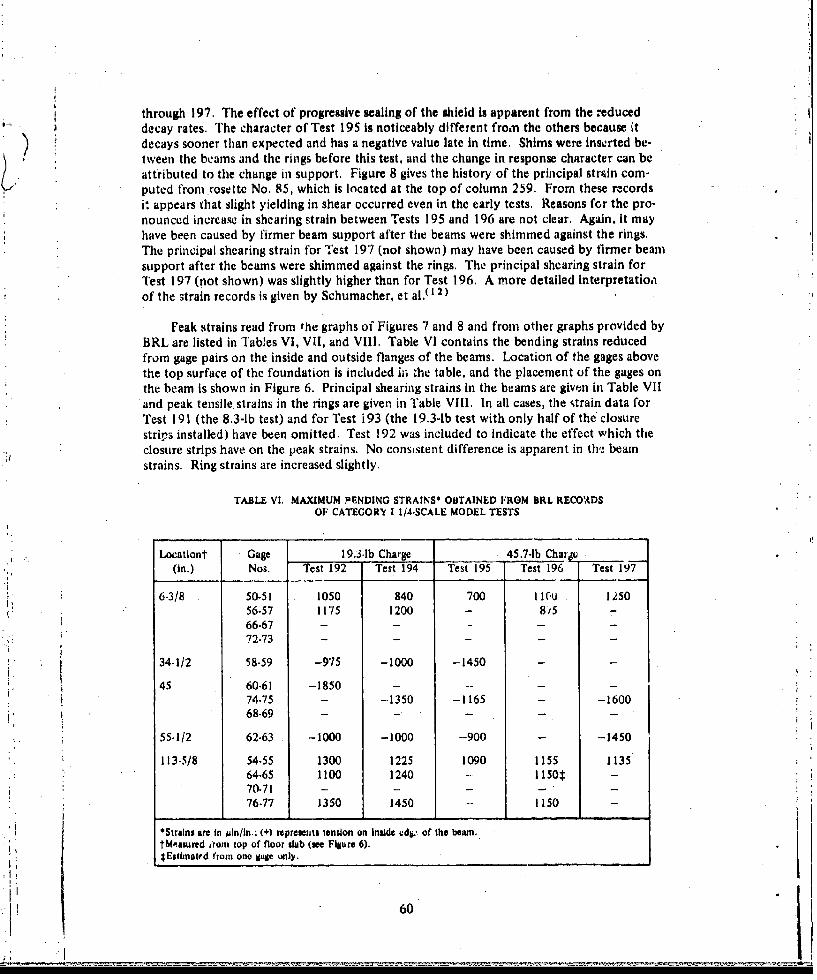
Feak strains read from the graphs of Figures 7 and 8 and from other graphs provided byBRL are listed in Tables VI, VII, and VIII. Table VI contains the bending strains reducedfrom gage pairs on the inside and outside flanges of the beams. Location of the gages abovethe top surface of the foundation is included ii- .he table, and the placement of the gages onthe beam is shown in Figure 6. Principal shearing strains in the beams are given in Table VIIand peak tensile strains in the rings are given in Table VIII. In all cases, the strain data forTest 191 (the 8.3-lb test) and for Test i 93 (the 19.3-lb test with only half of the closurestrips installed) have been omitted. Test 192 was included to indicate the effect which theclosure strips have on the peak strains. No consistent difference is apparent in th'. beamstrains. Ring strains are increased slightly.

TABLE VI, MAXIMUM PENDING STRAINS* OBTAINED FROM URL RECOADSOF CATEGORY I 1/4-SCALE MODEL TESTS

Locationt Gage 19.3-lb Charge 45.7-lb Chr•i V(in.) Nos. Test 192 Test 194 Test 195 Test 196 Test 197

6-3/8 50-51 1050 840 700 1 I(u 125056-57 1175 1200 - 815 -

66-67 - - -

72-73 ....

34.1/2 58-59 -975 -1000 -1450

45 60-61 -1850 - -.74.75 - -. 1350 -1165 - -160068-69 .....

55-1/2 62-63 -1000 -1000 -900 -1450

1t3.5/8 54-55 1300 1225 1090 1155 113564-65 1100 1240 1150t: -

70.71 - -.76-77 1350 1450 -- 1150

*Strains are In Mmn/in.; (+) rcpreueints tension on inside iudg, of the beam."tMmzared irom top of floor slab (we Figure 6).jEstitmatrd from one gage only.

60 H

TABLE VII. MAXIMUM SHEAR STRAIN* OBTAINED FROM BRL RECORDSS~ OF CATEGORY I 1/4-SCALE MODEL TESTS

/'Louationt Rosette 19.3-lb Charge 4.-bCharge-

(ill.) No. Test 192 'Test 194 Test 195 -- 'e-st 1-96 Test 197

34-1/2 78 1700 2650 3250 -

8 1 - --.

113-5/8 80 ....- -.

83 2150 2000 2500 7500 -

84 -- 1550 2400 - -85 2800 2350 7000 14000 14810

*Strains are in lin/in.tMeasured fromr top of flhor slab (see Figure 6).

TABLE VIII. MAXIMUM RING STRAINS OBTAINED FROM BRL RECORDSOF CATEGORY I 1/4-SCALE MODEL TESTS

Gage 19.3-lb Charge 45.7-lb Charge

-Lncationt No. Test 192 Test 194 Test 195 Test 196 Test 197

Top Ring 90 -- 1060 2580 2400 220091 -1430 -- 3100 2400 4200

Middle 92 1450 1600 - 3300 3400Ritng 93 1150 2300 2800 2100 3100

"Strain. are in ti/lhin.

tSe. Figure 6.

B Cornparisons with Analytical Predictions

For comparison with the measured strains of Tables Vi, VII, and V1I1, strains in thebeams and rings were computed usiio, both the approximate energy procedures describedin Section ii and finite-element methods. Application of the eniergy inethods to computestructural response has been reported in References 1, 4, 7, 9, and 10, and in earlier chaptersof this report, so these energy methods will be used here with a minimum of explanation.

:1 Application of the finite element program to compute structural response will be describedmore thoroughly.

I. Predictions Using Approximate Energy Methods

a. Uncoupled Solution

The blast loads associated with a confined explosion as in a suppressive struc-ture are not the same as the blast loads associated with an unconfined explosioll. Initially ina confined explosion, a shocK wave is propagated out away from a source; however, because

61

of the walls in the container, this initial shock is reflected many times until through variousdissipation mechanisms, the air is heated and a static pressure buildup of very long durationresults. In the suppressive structures program, this multiple loading mechanism was mathe-matically modeled by treating the initial shock wave as a delta function (as an impulse) andthe long duration buildup of internal pressure as a constant static pressure.

The generalized solution for the response of a beam in bending to this type ofloading is given in Figure 4 of Chapter Hl. As in all solutions for structural elements: idealboundary conditions are assumed, and coupling between the element and its supportingstructure are neglected. For the Category I model, the assumption of clamped-clampedboundaries for the beams is most appropriate.

Beams in the model are S3 X 5.7. Properties of the beam cross-section areobtained from the Steel Construction Handbook and the remainder of the beam geometryfrom Figure 5. Loads on the beam are produced by the initial reflected blast wave mad bythe subsequent quasi-static pressure. Impulse in the blast wave is obtained from the datapresented by Baker! . 3) The quasi-static pressure is determined using the procedure developedby Baker, et al./ ) Compiling the input data for Figure 4 from the above hources, we have

Geomctry:

A = 1.67 in. 2 (area of the beam)

b = 1.43 in. (loaded width-less than flange width because of overlap)

H = 3.0 in, (beam depth)

z = 1.95 in.3 (beam plastic section modulus)

1= 1.65 in.4 (beam elastic section modulus)

ay = 45,000 psi (material yield strength)

E = 30 X 106 psi (elastic modulus)

p = 7.33 X 10- lb-sec 2 /'n.4 (material density)

Loading Parameters:

19.3-lb Charge 45.7-lb Charge

Reflected impulse, 1, = 0.20 psi-sec 0.48 psi-see

Quasi-static pressure, P., = 73 psi 190 psi

A yield strength greater than the minimum guaranteed for the material was chosen becauselimited measurement on structural steel conducted during the suppressive structures programshowed yield values between 40.000 psi and 50,000 psi.

Maximum ueam strain for the 45.7-lb charge weight was computed in Chapter11, Part D, as an example for the use of Figure 4. The calculated strains given in Table IX wereobtained using the same procedure for the loading produced by the 19.3-lb charge.

62

TABLE IX. COMPARISON OF PEAK BEAM BENDING STRAINS:EXPERIMWNT TO UNCOUPLED ENERGY SOLUTIONS

Charge Weight Calculated Measured(lb) Wde) (e)

19.3 3,730 1450

45.7 32,700 1600

For the 19.3-lb charge, data from Test 194 rather than Tlest 192 were used. The peak strainoccurred at the top of an inside beam. For the 45.7-lb charge, the maximum measured strainwas midway between two supports (two rings) on the same beam. The gages which recordedthe maximum strain for the 19.3-lb charge were no longer operative for the tests with the45.7-lb charge, so bending strains at the top of the beam might have been greater. Even ifthis were so, it is apparent that the predicted strains are much larger than measured values.This is particularly true for the 45.7-lb charge.

The predictions of Table IX were obtained by, in effect, treating 'he rings asrigid and aborbing al! of the energy produced by the blast in the beams only. Obviously,these predictions ate much too constrvative to be of practical use in shield design. Similarly,ring response, computed for the assumption of rigid beams, is much tco great. Thus, theenergy absorbed must be properly divided betweLn the beams and the rings, and this requiresa coupled solution,

b. Coupled Solution

A solution for the coupled response of two structural components, one sup-ported by the other, is described in Chapter I! and Reference l0. It assumes rigid-plasticbehavior with loads applied to the supported structure only. The loading is comprised ofan initial impulse and a quasi-static pressure as for the uncoupled solution described previously.For beanms supported by rings (hoops) as in the Category I shield, the response of the systemis given by Eq. (64) of Chapter 1I. This equation, repeated here for convenience, gives themotion of the center of the beam, w0 , relative to the rings.II

I-.ub -

-,.1 pb2a NpbAb? \ohAhA -a IpbAbQ 1

_ohAh__ 1

pbA/jUbZWt N~b2 41rph AR h 2rb ] + 2N rq42uhh~l [1 ojhZR ,L J

(64)

Once wo is found, Eq. (59), also taker. from Chapter I, gives the total radialmotion, AR, of the ring in terms of w0.

pJAhR p&,rQ___ N b 2oh,, (59)AR Nbz

2 63 -liIi IA aAh Q

63

Based on the maximum deflections, wo ard AR of the beam and ring respectively, the residualstrains aie computed from Eqs. (65a) and (65b).

AR, -(65a)R

7r 2 IV,/Eb = f- (65b)

To compute residual strains in the Category I 1/4-scale model using these

equations, the following parameters are required:

ab = oh = 45,000 psi (material yield strength)

Pb = ph = 7.33 X 10-' lb-sec2 /in. 4 (material density)

Ab = 1.67 in.2 (beam cross-section area)

z = 1.95 in.2 (beam plastic section modulus)

N = 296 (no. of beams supported by the rings)

b = 1.43 in. (beam loaded width-less than fiange width because of overlap)

R = 30 in. (beam length)

H = 3.0 in. (beam depth)

Ah = 5.625 in.2 (one-half of the ring area)

R = 72.25 in. (radius to center of the ring)

r = 67.25 in. (internal radius of:the shield)

Blast loads are the same as listed on page 62.

Results obtained with the coupled solution are compared to the experimentin Table X. Both beam and ring strains are included. Calculated strains are residual, whereasthe measured strains, are peak. It is not appropriate to simply add the elastic strain at yield(ey = y/IE = 1550 m/in./i) to the residual strain, but the peak strain would lie between theresidual strain, e,, and the residual plus elastic strain (6r + ec). With this in mind, the agree-ment between the calculated and measured strains is good. Very little yielding, if any,occurred in the beams, and this is predicted by the analysis. Predicted ring strains are higherthan measured for the 45.7-lb charge. One reason for this may be that the nine individualbands from which the ring was assembled were not in good contact. This means that higherstrains occurred in the inner bands than in the outer bands where the measurements weremade. Also, many rings broke near the welds, which may indicate an embrittlement problem.

64

- - -.-- - - - --- - - - -- -~--.- ---- ---- ---~. . . .

TABLE X. COMPARISON Or BEAM AND RING STRAINS:EXPERIMENT TO COUPLED ENERGY SOLUTIONS

19.3-lb Charge 45.7-lb ChargeStructural Calculated Measured Calculated Measured

Component Residual Wpe) Residual (Oe)_(•e) (te)

Beams 200 1450 390 1600Rings 975 2300 6,880 4200

As can be seen by comparing the results in Tables IX and X, the use of couplingis to greatly reduce the calculated estimates. Although the estimates are still not in perfectagreement, the coupled predictions are much closer to measured values than are the uncoupledpredictions. Even better prediction should be achieved with finite element methods.

2. Predictions by Finite Element Methods

In addition to the energy solutions, a small two-dimensional (2-D) finite elementcomputer program, developed specifically for the dynamic-transient analysis of beams toblast loading, was used to predict structural response of the Catego,'y I 1/4-scale model. Theequations of motion art cast in finite difference form and integrated step-wLe in time usinga predictor-corrector method. The program treats material behavior as bilinear with hystereticrecovery, including the effects of strain rate and strain hardening. Calculations of the responsewere made with and without strain rate to show the significant effect strain rate has on dis-placements and strains. Strain hardening effects were found to be negligible and are not dis-cussed further.

The finite element model used for the calculations is shown in Figurk; 9. It is drawnschematically alongside one of the beams from the cylinder. The structure is idealized byassuming axial symmetry and symmetry about a horizontal plane through the center of theshield. This amounts to neglecting the presence of the door on the response of the beamsaway from its immediate vicinity, and neglecting axial loading and response. Although thereis some connection between the beams through the closure strips, which are tack welded tothe face of the inner beam and to the studs on the outer beam (see Figure 5), the beams are

p assumed to respond individually. Thus, only the lower half of one beam is represented inthe model.

Bilinear springs have been used to model the rings and radial flexibility in thefoundation. The resistance of the rings is divided into two parts to spread the support overthe ring width. Guided end conditions permit lateral displacements, but no rotation, andthe first beam element above the foundation has been sized to represent the combined bendingstiffness of the slab foundation and the bolted connection. Although the closure strips maycontribute to the beam stiffness, they are not welded continuously to the beams, and so thiscontribution is ignored; however, mass of the closure strips and the liners is added to thebeam mass.

65

1) Cnt~w ~ l.I % .- ~Guidad EndCenter ... • Shield CL Canditfun (typ)

Vn

Beam Element

Bl-linear

Spring

LoowdrRing

Lumped Mass

Fouidsiaton

FIGURE 9. SCHEMATIC OF THE FINITE ELEMENTMODEL OF THE STRUCTURE

66

As for the energy solutions, the pressure loading was assumed to be uniformly dis-tributed over the beam. The loading is composed of an initial Impulse and near constant(quasi-static) pressure. Two load cases were analyzed. They are the same as listed on page

19.3-lb charge: ir = 0.20 psi-sec

Pqs = 73 psi

45.7-lb charge: I, = 0.48 psi-see

Pqs = 190 psi

Basic beam and ring parameters used in computing input for the program are:

* S3 X 5.7 beam geometry

* mass per unit length (including closure strips and liners),A = 1.46 X 10-3 lb-sec/in.2

* foundation effective modulus, E, = 4.5 X 106 psi

* beam plastic moment, My = 87.750 in./Ilb

* beam elastic modulus, E = 29 X 106 psi

a beam plastic modulus 1% of elastic modulus

* beam loaded width, b 1.43 in.

Although the details will not be given, stiffness of the reinforcing gussets at the foundationand of the spacers at the rings was added to the beam. Also, estimates were made of thebending stiffness of the beam attachment to the foundation. Strain rate effects are basedon the well known relationshipC141 for mild steel given in Eq. (153)

where Od is the dynamic yield stress, and • is the strain rate.

Results for the 19.3-lb charge are given in Figure 10. Strain rate effects are included.This figure shows the distribution of maximum values of displacement, bending strain, andshear stress along the beam. The shear stress is based on the shear reactions in the beam ratherthan on shearing strains, and is computed as

V(154)

where V is the shear reaction in the beam, d is the beam depth, and t" is the beam web thick-ness. Data points are shown as circles. Three observations can be made from this comparison:

(I) The distribution of peak strains in the beam is irregular and not what onewould expect if only a section of the beam between two rings were analyzed.

67I .

Z Shear Stress, r1 (kni)-40 -30 -20 -10 0 10 20 30 40

I ("I I I ICL

IJ

+t1Sbr

V 0

Strain Gages (typ) "36 ~ '

0 ~

0

28 -0

* +v tension on outersurface of thebe.am

Measured Strain(typical)

-4000 -2000 0 2000 4000

Reinforced Strain, q (Vin. /in.)Concrete

Foundation I •-0.4 -0.2 0 0.2 .0.4

Radial Displacement, 6 r (in.

AND SHEAR STRESS VALUES (19.3 lb charge)

68

(2) Computed results for bending strains underestimate the measured values forthis charge weight (at the measurement location).

(3) If the computed distribution of strain is accurate, the measurement pointmay not have recorded the maximum values.

Figure I I gives similar results for the 45.7-lb charge. The same observations canbe made for this case as were made for the smaller charge excepi that, in thi3 instance, thecomputed strains are higher than measured valves. Also, for this charge weight the shearingstresses exceed the shear yield stress of the material at many points along the beam. Weestimate that the allowable shear stress values for the material are:

y --21,600-27,000 psi

a = 34,800-49,800 psi

These compare to peak calculated values; of 44,000 psi, which indicates that substantialyielding of the beam in shear should 1, ave occurred, and perhaps the beam was near shearfailure.

Although strain comparisons cannot be made because shearing strains were notcomputed by the program, Table XI lists measured .hear strains versus the computed stress.The measured results confirm that substantiz] yielding occurred in shear for the 45.7-lbcharge. Shear strains slightly beyond yield were also recorded for the 19.3-lb test. Theseresults, plus the results in Figure 1 1, indicate that the beam is not properly proportionedfor I :.;hly impulsive short duration loading. Higher shear area relative to bending stiffnessis needed to bring the sheariig and bending strains into better balance. This observation istrue for almost all commercially available beams b.•:cause they have been designed for highef .iency under static loads.

TABLE XI. BLAM SHEAR DATA

19.3-lb 4,,.7.lbMeas. Cale. Calc.

Location Mtas. Stres Measured Strain StresStrain Stress Stress

Test 194 F.E. Prog Test 195 Test J96 Test i97 FE. Prog

Outer beam 34-1/2"from foundation 2,650* 18,00ot 3,250 .... 35,000

"Outer beam 6-1/4"

from roof 1,550 20,000 2,400 .... 44,000

Inner beam 6-I/4"from roof 2,000 20,000 2,500 7,500 .- 44,000

Inner beam 6-1/4"

from roof 2,350 20,000 7,000 14,000 14,800 44,00(C

*Strain in./in. !', - tStrcss psi. _

69

- Shear Stream, w (keil-50 -40 -30 -20 -10 0 10 20 30 40 50

CL 60

0 0/- "-°52 ° /

k ,'tpical

• 'ft /

IFI

-4000 -200 0 V0 200 40I

S• • "P~it envion on outer.

Sllsurtare ot :he,

Measured Strainl

i t p c l -... .-oo .. o ..o ..oStrain, qg Lin./in.)

roindatlon r 1 4 0. 6

-0.4 -0.2 0 0.2 .4 0.6Radial Dim.lacement, 6.. (ix.

FiGURE 11. DISTRIBUTION OF MAXIMUM DEFLECTION1, STRAINAND SHEAR STRESS VALUES (45.7 lb chax•W'

70 ** "

UI

Only results which included strain rate effects were presented in Figures 10 and I .The effects of strain rate on the overall structural response are best demonstrated by the variationin ring strains. Measured ard calculated strains are given in Table XII. Calculated values includethose obtained by energy formulas as well as by the finite element program. For the energysolutions, both coupled and uncoupled results are included. The coupled solution was obtainedfrom Eqs. (59) and (64); the equation for uncoupled response is given in Table IV of Chapter III.

TABLE XII, MEASURED AND CALCULATED STRAINS IN THE RINGS

19.3 lb 45.7 lbTest 194 Test Test 196 Test 197

Top PingMeasured

Gage 90* 11001. 2200 2400 2200Gage 91 -- .,I00 2400 4200

F.E.f SolutionNo S.R.** 5315 13630

With S.R. 1840 5110 1

Energy FormulasNo coupling 3100 18490With coupling 2460 6320

Center RingMeasured

Gage 92 1600 3300 3400Gage 93 2300 2100 3100

F.E. SolutionNo S.R. 10360 21530With S.R. 3000 9740

Energy FormulasNo coupling 3100 18490With couphing 2490 6824

"Rkefer to Flguw - 7 for gage locations.+Stralr.s are in p in./in.:Finite element 2-D proglmf."*Strain rate effects.

The most obvious conclusion to be reached from the results in Table XII is thatthe calculated values overestimate measured ring response in every cese. For the two com-parisons available, it appears that the difference between computed and mneasured valuesincrea•ses as charge weight increases: hence, the analytical results should always be conservative.The effects of strain rate and coupling are pronounced, reducing calculated values by approxi-mately a factor of three for the large charge weight. Still, the calculated values aie far abovemeasured values. It should be noted that the energy solution does not include strain rate orstrain hardening effects and yet gives a result which is the same order of magnitude as the

71

II71

-~ more rigorous finite element method. One reason for thls is that the ene~rgy solution forcesplastic deformation in the beams, whereas the finite element solution does not. It is apparentfrom Figure I I that predicted plastic straining In the beams was minimal so that energy absorp-tion by the beams was small.

Reasons for. the disagreement between predictions and measurements of ringresponse are rnot clea,. -However, two factors may have affected tile rc`Lrlts:

(1) YThe closure strips shown in Figure 5 were tack welded to the inner beams andprovided some circumferential restraint. Thus, the closure strips acted in amanner similar to rings, but were distributed over the full height of the shield.This effect was neglected in the response calculations.

(2) Properties of the rings material were never measured. It proved to be a brittle

material because fractures were noted during the testing. The calculatior~swere performed Lassuming a mild steel, which may not represent true ring

properties.

One final comparison of measured and calculated results is given in Table X1II. Itcompares peak meastired strains in the beam to strains and shearing stresses computed byboth the energy and tinite element methods. From this comparison, it is obvious that boththe finite element solution with strain rate effects and the coupled energy solution give resultswhich are cutisistent with the measured values. Additionally, the finite element method pro-vides useful information on shear in beams by providing shear reactions which predict thepresence of lirge shearing strains. From the finite element solution, it is also apparent thatstiairi rate effects play little part in the beam bending response. By stiffening tnc ring, how-ever, strain rate does cause higher shear stresses. This stiffening of the ring was demonstratedin Table XII by the sharp reduction in the ring strain.

TABLE XIII. COMPARISON OF PEAK VALUES IN THE BEAMS

19.3l1b ch rge 45.7 lb charge_____Bending Shear Shear Bending Shear ShearStrain Strain Stress Strain Strain Stressju in./in pi in./in. psi y in./in. p in./in. psi

Measured 1450 2650 1600 14,800

F.E. MethodNo SR **.3010 36,900With SR 1400 20,000 3000 44,000

Enorgy Solution

Uncoupled 3730 12700Coupled 2 00 390(Residual) ________________________ ____________

72

C. Conclusions from the Strain Data Analysis

The conclusions drawn troam these comparisons of analysis and experiment are:

(1) Strain data, provided by BRL in the form of computer generated plots, appear tobe good. '[he data lire surprisingly consistent from test to test for a structure whichwas being altered continuously. and undergoing.pla-'tic strains. Exceptions occur,and these can usually be explained by major alterations to the structure, such asshimming the beams prior to Test 195.

(2) Measured beam bending strains are lower than expected and did not increase sig-Swficantly with an increase in charge weight.

(3) Shear strains in the beam web were high. Yielding occurred as predictud by highshear forces which were calculated for the beams.

(4) Ring strains were much lower than predicted, particularly for the large chargeweight.

(5) The comparisons show that the energy solution for coupled responsý carn givereasonable answers, which, if in error, tend to overestimate the strains.

(6) The finite element computer solutions show that strain ral.e should not be ignoredin structural componenis which respond primarily in a stretching mode, such as forthe rirgs. If these effects are ignored, the solution is an upper bound, but it is tooconservative to be useful if reasonably accurate predictions are desired.

V. PRESSURES FROM BURNING PROPELLANTW IN VENTED CHAMBERS.

The thrust of this effort was to determine theoretically the peak quasi-static pressure• "produced by burning M 10 propellant in closed and vented chambers. Combustion equations

were written to define the heat generation and products of the burning propellant which actto increase the pressure in the shield. Temperature and pressure increases in the shield pro- '1duced by burning the propellant are offset by radiation to the shield Walls and gas flow fromthe shield through the vented panels, The equations describing these processes were codedinto a computer program called GASSS which performed the calculations for MIO propellantburned in a Category V shield. "

A. Combustion Equations

M 10 propellant is 98, nitrocellulose with 13.15% nitration. Other major constituents

are potassium sulfate and diphtnylamine. Since nitrocellulose is the most active element inthis propellant and since most of the propellant is nitrocellulose, the program assumes thatMI0 is all nitrocellulose. Thus, our calculations for energy produced from burning the pro-pellant will be an upper limit. Based on 13.15% nitration of nitrocellulose and informationin the literature on its products of combustion,"t 5) the reaction equations for burning nitro-cellulose in the absence of air are:

73

C6H7(NO2 i;. 6 3 05 -1.556CO + 4.407 CO + 1.001 H2 + 1.297 N2 +2.6221 H20

+ 265.0 kilocalories (155)

Secondary reactions involving the combustion of CO and H2 in air are:

CO + l/202 -'CO2 + 67.63 kilocalories (156)

and

H2 + 1/202-HaO + 57.80 kilocalories (157)

The program was written so thai during each time step, the products and energy of thereaction are calculated first without the presence of oxygen. Then, a calculation is performedto determine the amount of oxygen available. If there is sufficient oxygen present, the secon-dary reactions take place. When the ow:ygen in the chamber is depleted, only the primaryreaction takes place. In vented and closed chambers, it is assumed that no oxygen entersfrom outside the structure due to positive pressure inside the chamber. The computer pro-gram also records the quantity of different gases present in the chamber at all times.

B. Gas Flow Equations

Determination of the pressure histoy for venting in a supprossive structure was accom-plished by assuming quasi-steady, isentropic flow of a perfect gas. A check on the reliabilityof the perfect gas assumption was made by assuming complete combustion in an unventedchamber with no energy loss, and thermal equilibrium in the gases. Pressure was calculatedusing the ideal gas law and also using Van der Waals equations for non-ideal gases, and theresults were compared. For the pressures and n.olecular quantities involved, the ideal gaslaw was found to be quite accurate.

For the calculated pressure dissipation, the suppressive structure was idealized as twocompartments separated by some vent area. If the ratio of atmospheric pressure to chamberpressure is less than

then supersonic flow equations are used. Otherwise, subsonic flow equations are utilized.The program causes the gas to vent proportionally to the quantity of each gas present.

If the flow is supersonic, the mass flow rate is determined by• 16)

At R1 T1 /g 7+

A CjAP 1,1 [ 2y(587)

741.

where

A = vent area of passage out of chamber

CD = discharge coefficient of area A

P, = compartment pressure

R = universal gas constant

T = gas temperature

g = gravity constant

- = ratio of specific heats

If the flow is subsonic, then

Amt"=CD I "[g F~a,,2/,y [at (,Y+1),

-- C- A 2g- -T•P i'" ) t P2,, (159)

where

P, density of gas in the chamber

P 2 pressure outside the chamber

The rate of temperature change is given by

. Tlt(7 1 )- flt , (160)= 1 M,(,t

"where

m = mass of the gas in the compartment, and the rate of pressure change is given by

RT 1 .rt, r1 P,P1, V - '- - +P -2 T (161)

,V TIj

where

I' = volume of the compartment. IP: Pressure and temperature in the initial compartment at t :t + At will then be

•" Pitr + at I ýPiAt +P1' I

L (162)

ST1j • at ij + A•At + T1,t

Pressure and temperature coutside the chamber were assumed to remain at ambient values.

75

C. Effects of Burning Rates and Radiant Heat Loss

Insufficient data were available to determine accurately the burning rates of piles of M 10propellant. A telephone conversation with Mr. William Seals,(17) of Picatinny Arsenal, pro-duced the following results for M10:

Burning Rate (in./&ec)

Pressure (psi) Single Perforation Multi-perforation

5,000 1.49 1.389,000 2.24 2.07

11,000 2.58 2.18

These burning rates are obviously appropriate for interior gun ballistics, but are not appropriatefor our purposes because the pressures in the suppressive structure for the worst case (no energyloss and instantaneous burning) are much smaller than the pressures in the table above. Measure-ments that Dr. Gary McKown€ 18 ) had taken when burning large quantities (500-1000 lb) ofsmoke mixes indicated burning rates of about 10 lb/sec. Measurements which he had takenwhile burning 10- and 50-lb quantities of magnesium and sodium nitrate illuminant producedburning rates varying from 4 to 100 lb/sec, depending on the quantity burned and the degreeof confinement.

In view of this uncertainty in the burning rate, various rates were used in the calculationsto show their influence on peak pressures in the Category V shield. Initially, burning rate wasdefined in units of lb/sec, and the pressure histories in the shield were computed using variousquantities of propellant, several different burning rates, and various effective vent areas. Theresulting pressures seemed to be unrealistically high, and this approach appeared to be inaccuratesince the burning rate should depend on surface area and ambient pressure, and there should beradiant energy loss depending on the burning surface temperature and area. Thus, the computerprogram was modified to incorporate a linear burning rate and radiant heat loss. Because of therelatively low peak pressures, we neglected pressure dependency of the burning rate.

To convert a linear burning rate to a mass burning rate and burning surface area requiredthat a burning geometry be assumed. Further, it was necessary that the burning surface besmall initially and increase with burning time, which is characteristic of point ignition. Thesimplest geometry which could be assumed was a sphere with point ignition at the center. Topermit radiation the sphere was treated as two hemisplieres. For this geometry the effectiveincrease in surface area with time is equal to that of a radially expanding sphere. The largestburning surface obtained in using this procedure is nearly identical to that of a cube of pro-pellant of equal weight with one face unexposed; that is, on the floor. For example, equatingvolumes of the sphere and cube:

4.R3 =(163)3

where R = radius of sphere (maximum)9 = edge of cube

"76

Solving Eq. (163) for R, one has

R 3 1/3 (164)

The maximum surface area of the sphere Is

Oirr= ~41r (i 9/ 2 ~4.84R2 (165)

which is nearly the area of the five exposed sides of a cube of identical weight.

The above assumptions on bulk propellant burning and increase in burning surface weremade to simplify a very complex burning process and provide for a reprasentative increase inburning surface area and attendant increasing radiation losses after ignition. The u'se of aspherical geometry to describe the burning process offers the advantage of simplicity. !t alsoallows for point ignition and growth in burning surface to a final value which is ntarly thesame in area as the exposed surfaces of a cube of equivalent weight. Thus, the simplifiedspherical geometry very nearly approximates the characteristics of the ictual burning process.

The computer program was changed to incorporate a radial burning rate (utmits of in./sec)for the bulk propellant. By assuming negligib!e pressure dependency (relatively low peakpressures) and spherical geometries, burning rates of 10 lb/sec translates to 3.41 in./sec,*7 lb/sec to 3.03 in./sec, and 4 lb/sec to 2.51 in./sec. The comp-:-ter program was also modifiedto allow for radiant heat loss from the burning propellant and radiation loss from the gas inthe chamber. Summaries of the output from these various techniques are contained in thetables that follow. The basic assumptions, in addition to the combus t ion and gas flow equations,are contained at the top of each table. We feel that the most accurate results are those whichallow for radial burning rates (especially 3.40 in./sec) and at least some radiant energy loss.We estimate that the Category V shield has an effective vent. area of 7.785 sq ft when vented.The effective vent area was determined by combining the vent areas of each component insidethe side and roof panels by the equation

I =i+ I+..+1 (166)Ntff til Or'2 an

where

Nff = effective vent area

(1 , a2 ... an = vent area of each componert

*Time for burning various quantities (assuming spherical geometries) can be calculated from

(3 A 113

IT Gs. 0.0602 lb/in.')r

where M Is the mass of the propellant In pounds, and r is the burning rate in inches/scond. For 3.41 In/nc burning rate,one can calculate that 10 lb burn- In 1.00 socond. 100 lb in 2.15 weconds,-and 1000 lb in 4.64 seconds.

77

The side panel consists of

0 a layer of angle irons with a vent area of 273 in.2 ,V a

0 a layer of angle irons with a vent area of 485 in. 2 ,

0 three perforated plates with each plate having a vent area of 1410 in. 2 ,

* four layers of aluminum mesh with each layer having a vent area of 3089 in.'.

Thus, from Eq. (166), the effective vent area of a side panel is

1i 1 1 1

A V panel 273 485 1410 3089

side panel = 109 in, 2

where A v side panel ie the effective vent area of a side panel.

The roof panel consists of

• a layer of angle irons with a vent area of 154 in. 2 ,

* a layer of angle irons with a vent area of 273 in.2 ,

0 three perforated plates with each plate having a vent area of 795 in. 2 ,

0 four layers of aluminum mesh with each layer having a vent area of 1742 in. 2 .

Thus, from Eq. (166), the effective vent area of a roof panel is

I 1 1 3 4A V roofpanel 154 273 795 1742

Avroof panel 61.6 in .2

where A Vroof panel is the effective vent area of a roof panel.i,

Accounting for eight side panels and four roof panels, the total effective vent area of theCategory V shield is

(8)(109.3) + (4)(61.63) " .785 ft2A V T 144

Figure 12 was taken from the numerical results contained in Table XIV and containsplots of peak pressure versus vent area for a burning rate of 150 lb/sec, no radiation loss, and

78

I

I I I I I I I I I

L Ill

0'0

.0

.0 ZI-.

U�i � 5

0.0 eII II II II II II 00

� � �oQ

00..0

'I I

0

- 0ir� � ,4. sj.� 0

(Ijud) 9Jnu�JJ 'I'�dK.. o

79

TABLE XIV. MIO PROPELLANT IN VENTED CHAMBER WITHNO RADIATION LOSS

SAssumptions: Ambient Pressure = 14.7 psiInitial Ratio of Specific Heats w 1.4Ambient Temperature = 77 0FChamber Volume = 919.6 cu ftNo radiation lossConstant mass/time burning rate

Run Effective Burning Quantity PeakRn. AT(sec) Vent Area Rate Pressure RemarksNo. (sq ft) (lbs/sec) (Ibs) (psi)

1 0.001 -0- 150 10 86 @ 0.067 sec2 0.001 -0- 150 50 372 @ O.100 se3 0.001 .0- 150 100 535 @0.334 sec4 0.001 0.006 50 10 86 @ 0.200 sec5 0.001 0.006 50 30 235 @ 0.600 sec6 0.001 0.006 50 50 >368 max. not reached7 0.001 0.006 50 100 >368 max. not reached8 0.001 0.006 100 30 236 @ 0.300 sec9 0.001 0.006 150 10 86 @0.067 sec

10 0.001 0.006 ISO 30 236 @ 0.200 sec11 0.001 0.006 150 50 371 @ 0.334, sec12 0.001 0.006 150 100 530 @0.667 sec13 0.001 0,006 300 30 237 @0.I00 sec14 0.001 0.18 7 10 48 max. not reached15 0.001 0.18 10 10 67 max. not reached16 0.001 1.2 150 10 77 @ 0.067 sec17 0.001 1.2 150 50 173 @ 0.255 sec18 0.001 1.2 150 100 173 @0.255 sec19 0.001 2.4 150 10 69 @ 0.067 sec20 0.001 2.4 150 50 108 @ 0.203 sec21 0.001 2.4 150 100 108 @0.203 sec22 0.001 4.71 10 10 3 @0.120 sec23 0.001 4.71 10 50 3 @0.120 sec24 0.001 4.71 10 100 3 @0.l 20 sec25 0.001 4.71 50 10 24 @ 0.136 saec26 0.001 4.71 50 30 24 @ 0.I 36 sec27 0.001 4.71 50 50 24 @0.136 sec28 0.001 4.71 50 100 24 @0.136 sec29 0.001 4.71 100 10 44 @ 0.100 sec30 0.001 4.71 100 30 45 @0.121 sec31 0.001 4.71 100 50 45 @0.121 sec32 0.001 4.71 100 100 45 @0.121 sec33 0.0005 4.71 124.4 10 51 @ 0.080 sec34 0.001 4.71 124.4 10 51 @ 0.080 sec35 0.005 4.71 124.4 10 49 @ 0.080 sec36 0.01 4.71 124.4 10 46 @ 0.080 sec37 0.001 4.71 124.4 50 54 @0. 117 sec38 0.001 4.71 124.4 100 54 @0.117 sec

80

TABLE XIV. MIO PROPELLANT IN VENTED CHAMBER WITHNO RADIATION LOSS (Cont'd)

Run Effective BuminP Quant rsur PeakNo, .AT(sec) Vent Area Rate (bs) Pressure Remarks

(sq ft) (Ibs/sec) (psi)

39 0.001 4.71 150 10 55 C' 0.06b sec40 0.001 4.71 150 30 63 @ 0. 113 sec41 0.001 4.71 150 50 63 Ca' 0.I13 sect42 0.001 4.71 ISO 100 63 (d 0.113 sec43 0.001 4.71 300 10 69 @ 0.033 see44 0.001 4.71 300 30 108 @ 0.100 see45 0.001 4.71 300 50 108 @ 0.103 sec46 0.001 4.71 300 100 108 @0.103 sec47 0.001 7.2 150 10 43 @ 0.066 sec48 0.001 7.2 150 50 44 @ 0.079 sec49 0.001 7.2 150 100 44 @0.0 7 9 sec

10-, 50-, and 100-lb quantities. Figure 13 was taken from the numerical results contained in

Table XV and contains a plot of peak pressure versus vent area for a radial burning rate of

3.41 in./sec and radiation loss from the burning surface and surrounding gas. Figure 13 is

for I 0-lb quantities and probably predicts peak overpressure more accurately than Figure 1 2.

Note that in the tables and figures, pressure is in units of psig; that is, pressure above atmos-

pheric pressure,

TABLE XV. MI0 PROPELLANT IN VENTED CHAMBERWITH RADIATION LOSS

Assumptions: Ambient Pressure = 14.7 psiInitial Ratio of Specific Heats = 1-4

SAmbient Temperature = 770FChamber Volume = 919.6 cu ftRadiation from produced gas and surrounding gasConstant Radid Burrdng Rate

Effective Burning Quatity PeakAT (sec) Vent Area Rate Pressure Remarks

No. (sq ft) (ln./sec) (psi)

1 0.005 0.18 3.41 10 60 @ 1.00 see2 0.01 0.18 3.03 10 57 @ 1.13 se3 0.01 0.18 2.51 10 53 @ 1.36 sec4 0.01 0.3 3.41 10 55 @ 1.00 sec5 0.01 0.6 3.41 10 43 .@ 1.00 see

6 0.01 0.6 2.51 10 33 @ 1.36 see7 0.01 1.2 3.41 10 25 @ 1.00 sec8 0.01 1.2 2.51 10 16 @ 1.36 sec

9 0.01 2.0 3.41 10 12 @ 0.90 sec10 0.01 4.0 3.41 10 2 @ 0.73 seeI 1 0.01 4.71 3.41 10 1.4 @ 0.70 sec12 0.01 4.71 3.41 50 1.4 @ 0.70 sec

13 0.01 4.71 3.41 100 1.4 @ 0.70 see

81

00*

t- 0 :F

E& m:j

eq U

CD. cm

(216) O~ss~l 180

8-J

D. Comparison with Experimental Results

Several tests have been conducted at NSTL where M I0 propellant has been ignited insidea Category V suppressive structure. Although a written report has not yet been publishedDr. Gary McKown of NSTL has revealed to us in a telephone conversation 18) that uncon-fined MI0 propellant is a slow burner. During the Category V tests, 100-, 250-, and 600-lbquantities of M 10 were burned inside the structure. The propellant was in cardboard boxesno more than a foot tall and was ignited from the top. The material burned like a "slowcandle," with a burning time of approximately two or three seconds, depending on theweight of the propellant. It also appeared that the burning rate varied linearly with themass of propellant.

During the tests there were large fireballs, no detonations, and very low quasi-staticpressures inside the structure. From the films of the event, it appeared as if either the pro-pellant or partially combusted products of the reaction had gotten outside the suppressivestructure and ignited, thus contributing to the enormous fireball. Also, during the tests,all of the aluminum screening inside the structure and portions of other aluminum componentswere burned out or deteriorated, possibly due to the intense heat of the reaction. For oneexperiment, the top of the structure was covered with a piece of steel to control the verticalflow of the fireball. This steel roof had a hole burned through it by the end of the tests.The maximum pressure recorded during the tests was approximately 0.2 psig. Most of thetime, however, pressure was so small that it was difficult to record.

As noted above, we suggested that Figure 13, with a radial burning rate of 3.41 in./secwhich reduces to 100 lb burned in 2.15 seconds, 250 lb burned in 2.92 seconds, and 600 lbburned in 3.92 seconds, was the best figure to use to determine peak quasi-static pressure.From Table XV and Figure 13, for an effective vent area of 4.71 square feet and either 10,50, or 100 lb of M10 propellant, one can see that the peak pressure is 1.4 psig. The initialCategory V suppressive structure has an estimated effective vent area of 7.785 square feet.Since the interior alumin-im baffles deteriorated after a few tests, the effective vent areaincreased 16.5% to 9.069 ft2 . This new effective vent area was determined by eliminatingthe last term in the equations used to calculate the effective vent areas of the side panelsand roof panels. When one considers the effect of this additional vent area and the effectof energy losses due to burning of propellant outside the chamber, one would expect thatthe curve in Figure 13 is an upper limit conservative calculation. If these other terms, thatis, additional vent area and radiant heat loss, were introduced into the computer program,lower and more accurate predictions would undoubtedly have been produced.

VI. DISCUSSION

Suppressive shielding was developed to house hazardous operations at explosivesprocessing facilities. Should an accidental explosion occur, the shield is designed to containor sharply reduce the blast overpressures,thermal effects, and fragment hazards produced.Nearby operations are thus shielded from the detrimental effects of the accident.

To properly design a shield to attenuate or completely contain the products of theexplosion requires a knowledge of several complicated phenomena. These include:

83

I. overpressures inside and outside a vented enclosure producu by the detonation ofhigh explosive charges or by the burning of propellants,

2. fragments generated by the accident,

3. thermal environment produced by the accident,

4. transient loading on the structural compon-nts of the shield produced by theoverpressures, fragments, andt thermal environment.

5. elastic-plastic response of the shield to the transient loading,

6. resistance of the shield to fragment penetration, and

7. attenuation of thermal effects by the shield.

Other aspects of the design include problems of entry and exit (for per.onnel, explosives,and utilities), cleanup, weatherproofing, lighting, air conditioning, and economy.

All of these problems have been addressed during the suppressive structures program,but not all of them have been satisfactorily resolved. Prediction of the thermal environmentind its attenuation by the shild has received the Ilast emphasis. Most other aspects of the!esign have been investigated in some detail, and procedures suitable for sh eld design haveDeen developed: however, alraost all aspects of the design can benefit from additional research.

The work documented in this report addresses principally items 1,4, and 5. This workhas included further devclooments in the application of energy methods for the analysis ofstructural response to blast loading, comparisons between predictions of structural responseand test results, and predictions of pressure-time histories inside vented enclosures producedby burning propellant. The procedures developed for predicting pressures inside veniedenclosures produced by a burning propellant are applicable to the design of Category Vshields. Formulas and graphical solutions for structural analysis are applicable to the limitdesign of all shield groups.

Comparisons between analysis and experiment, which are described in this report andin earlier workt 1.4,61 have shown that approximate energy methods pro"de 63od estimatesfor the elastic and elastic-plastic behavior of simple structural elements subjected to blastloading. This report contains a comprehensive summary of solutions developed during thesuppressive stru, lures program for the analysis of a large number of different structuralelements. The comparisons also show that solutions for simple structural elements are notalways suitable for the analysis of complex structures. Coupling, which can occur betweenstructural components, can greatly attenuate the response of each component treatedseparately. However, even in this case we have shown that approximate energy solutionscan give good revults, but with some increase in complexity. Energy methods also lend then.-selves to graphical solutior.s which greatly simplify the complexity and labor involved in thtsolution process.

84

Although substantial progress has been made in the development of analytical pxcceduresto support the design of suppressive shields additional work is needed in several areas. Theseinclude:

I definition of the thermal environment produced by the detonation of a highexplosive or by the burning of propellant,

2. methods to predict the thermal environment outside of a suppressive shield,

3. comparisons between measured and predicted pressures produced by burningpropellants in vented enclosures,

4. failure criteria for dynamically loaded commercially available structural components.Cumm'ercially available components have been designed for optimum efficiencyunder static loading. A better understanding of their behavior when loaded byshort duration high intensity loads is needed. This is particularly true for thefailure-of wide-flange beams in shear.

"= i

85r

REFERENCES

1 W.E. Baker, P.S. Westine, P.A. Cox, and E.D. Esparza, "Analysis and Design of a Sup-pressi-ve Structure for a Melt Loading Operation," Edgewood Arstnal Contract ReportEM-CR-76056, Report No. 1, May 1976.

2. W.E. Baker and G.A. OIdham, "Estimates of Blowdown of Quasi-static Pressures inVented Chambers," Edgewood Arsenal Contract Report EM-CR-76029, Report No.2, Contract DAAA15-75-C-0083, SwRI, San Antonio, Texas, 1975.

3. E.D. Esparza, "Estimating External Blast Loads from Suppressive Structures," Edge-wood Arsenal Contract Report EM-CR-76030, Report No. 3, Contract DAAAI15-75-C-0083, SwRI,San Antonio, Texas, 1975.

4. P.S. Westine and P.A. Cox, "Additional Energy Solutions for Predicting Str'.lcturalDeformations," Edgewood Arsenal Contract Report EM-CR-7603 1, Report No. 4,Contract DAAA I5-75-C-0083, SwRI, San Antonio, Texas, 1975.

5. W.E. Baker and P.S. Westine, "Methods of Predicting Blast Loads In3ide and BlastLoads Outside Suppressive Shields," Edgewood Arsenal Contract Report EM-CR-76026,Technical Report No. 5, November 1975.

6. P.S. Westine and W.E. Baker, "Energy Solutions for Predicting Deformations in Blast-Loaded Structures." Edgewood Arsenal Contractor Report EM-CR-76027, Report No.6, November 1975.

7. P.A. Cox and E.D. Esparza, "Preliminary Design of a Suppressive Structure for a Melt"Loading Operation," Edgewood Arsenal Contractor Report EM-CR-76028, ReportNo. 7, Contract DAAA15-75-C-0083, SwRI, San Antonio, Texas, 1975.

8. E.D. Esparza, W.E. Baker, and G.A. Oldham, "Blast Pressures Inside and Outside Sup-pressive Structures," Edgewood Arsenal Contract Report EM-CR-76042, TechnicalReport No. 8, December 1975.

9. W.E. Baker, P.A. Cox, E.D. Esparza, and P.S. Westine, "Design Study of a SuppressiveStructure for a Melt Loading Operation," Edgewood Arsenal Contractor Report FM-CR-76043, Report No. 9, December 1975.'

10. P.S. Westine, P.A. Cox, and E.D. Esparza, "Structural Analysis Emphasizing EnergyMethods: Some Comparisons with Suppressive Shield Experiments," Minutes of the17th Explosives Safety Seminar, Denver, Colorado, September 1976.

1i. R.N. Schumacher and W.O. Ewing, Jr., "Blast Attenuation Outside Cubical EnclosuresMade Up of Selected Suppressive Structure Panel Configurations," BRL Interim Mem-orandum Report No. 376, April 1975.

12. R.N. Schumacher, C.N. Kingery, and W.O. Ewing, Jr., "Airblast and Structural ResponseTesting of a 1/4-Scale Category I Suppressive Shield," BRL Memorandum Report No.2623, May 1976.

86

13. W.E. Baker, Explosions In Air, University of Texas Press, Austin, 1973.

14. P.S. Symonds, "Survey of Methods for Plastic Deformation of Structutes UnderDynamic Loading," Department of the Navy, Contract NONR 3248(01)(X). NavalShip Research and Development Center, June 1967.

15. Jocelyn Field Thorpe and M.A. Whiteley, Thorpe's Dictionary of Applied Chemistry,Vol. IV, 4th edition, 1940, Longmans, Green & Co., London, pp. 506-516.

16. G.F. Kinney and R.G.S. Sewell, "Venting of Explosions," NWC Technical Memorandum

2448, Naval Weapons Center, China Lake, California, July 1974.

17. Telephone conversation with Mr. William Scals of Picatinny Arsenal.

18. Telephone conversation with Dr. Gary McKown, Edgewood Arsenal at the NationalSpace Test Laboratory (NSTL) in Bay St. Louis, Mississippi.

19. D.A. Martin and G.L. McKown, "Proof Testing of a Candidat, Category III SuppressiveShield," Edgewood Arsenal Tech. Report No. EM-TR-76064, August 1976.

8

I.

DISTRIBUTION OF SUPPRESSIVE SHIELDING REPORTS

Addressee No. of Copies

CommanderRocket Propulsion LaboratoryAttn: Mr. M. RaleighEdwards Air Force Base, CA 93523

CommanderHQ, Armament Development Test CenterAttn: DOM/Mr. S. ReitherEglin Air Force Base, FL 32542

CommanderHill Air Force BaseAttn: MMNTR/Mr. CummingsClearfield, UT 84406

CommanderNorton Air Force BaseAttn: AFISC-SEV/Mr. K. CollinsworthSan Bernardino, CA 92409

CommanderAir Force Civil Engineering CenterAttn: AFCEC-DE/LTC WalkupTyndall Air Force BasePanama City, tcL 32401

Commander I eaHQ Air Force Logistics CommandAttn: MMWM/CPT D. Rideout

IGYE/Mr. K. ShopherWright-Patterson Air Force BaseDayton, OH 45433

CommanderNaval Ordnance Systems CommandAttn: Code ORD 43B/Mr. A. FernandesWashington, DC 20360

Commander .1Explosives SafetyAttn: ADTC/SEV (Mr. Ron Allen)Eglin Air Force Base, FL 32542

88

CommanderBureau of Naval WeaponsAttn: Code Fl2/Mr. H. RoylanceDepartment of the NavyWashington, DC 20360

CommanderNaval Ship Research & Development CenterAttn: Code 1747/Mr. A. WilnerBethesda, MD 20034

CommanderNaval Explosive Ordnance Disposal FacilityAttn: Code 501/Mr. L. WolfsonIndianhead, MD 20640

CommanderNaval Ordnance Systems CommardNAPECNaval Ammunition DepotAttn: ORD-04M/B/X-5/Mr. L. LecnardCrane, IN 47522

* - CommanderUS Naval Surface Weapons Center

* Attn: Mr. J. ProctorWhiteoak, MD 20904

Chairman 5DOD Explosives Safety BoardAtMn: COL P. Kelly, Jr.Forrestal Building GB-270Washington, DC 20314

Joint Army-Navy-Air Force Conventional 5', • Ammunition Production Coordinating Group

USA Armament Command

Attn: Mr. Edward JordanRock Isl-nd, IL 61201

HQDA (DAEN-MCC-I/Mr. L. Foley)Washington, DC 20314

HQDA (DAEN-MCE-D/Mr. R. Wight)Washington, DC 20314

DirectorUSAMC Field Safety ActivityAttn: AMXOS-TA/Mr. OlsonCharlestown, IN 47111

89

Commander I etUS Army Materiel CommandAttn: AMCCG

AMCRDIDr. KaufmanAMCSF/Mr. W. QueenAMCPM-CS/COL Morris

5001 Eisenhower Ave.Alexandria, VA 22333

Office of the Project Manager for 3Munition Production Base Modernization

and ExpansionAttn: AMCPM-PBM.-E/Mr. DybackiUSA Materiel CommandDover, NJ 07801

Commander 1 eaUS Army Armament CommandAttn: AMSAR-EN/Mr. Amnbrosin

AMSAR-SC/Dr. C. HudsonAMSAR-SF/Mr. J. VarchoAMSAR-TM/ Mr. Serlin, Mr. T. Fetter, Mr. S. PorterAMSAR-MT/ Mr. A. Madsen, Mr. G. Cowan, CPT Burnisteel

Rock Island Arsenal* Rock Island, IL 61201

* Commander l agUSAMC Ammunition CenterAttn: Mr.J. Byrd

AMXAC..DEM/Mr. Huddleston

Savanna, IL 61074

*Commander l eaFrankford ArsenalAttn: Mr. F. Fidel, Mr. E. RemplerBridge and Tacony Sts.

Philadelphia, PA 19137

CommanderPicatinny ArsenalAttn: Mr. Saffian 3

Mr. J1. Cannovan I eaI Mr. HickersonMr. 1. Forsten

Dover, Ni 07801

90

CommanderUSA Test and Evaluation CommandAttn: AMSTE-NBAberdeen Proving Ground, MD 21005

Commander I eaDugway Proving GroundAttn: Dr. Rothenburg

Mr. P. MillerDugway, UT 84022

CommanderCornhusker Army Ammunition PlantGrand Island, NE 68801

CommanderIndiana Army Ammunition PlantCharieston, IN 47111

Commanderiowa Army Ammunition PlantBuilington, IA 52502

CommanderJoliet Army Ammunition PlantJoliet, IL 60436

CommanderKansas Army Ammunition PlantParsons, KS 67357

r- CommanderL Longhorn Army Ammunition Plant

Marshall, TX 75671

I CommanderLone Star Army Ammunition PlantTexarkana, TX 75502

CommanderLouisiana Army Ammunition PlantShreveport, LA 71102

CommanderMilan Army Ammunition PlantMilan, TN 38358

i CommanderRadford Army Ammunition Plan!Radford, VA 24141

91

CommanderSunflower Army Ammunition PlantLawrence, KS 66044

CommanderLake City Army Ammunition PlantAttn: Mr. John JacobiIndependence, MO 64056

CommanderRavenna Army Ammunition PlantRavenna, OH 44266

Commander jPine Bluff ArsenalPine Bluff, AR 71601

Director 3US Army Materiel Systems Analysis ActivityAberdeen Proving Ground, MD 21005

DirectorUS Army Ballistics Research LaboratoriesAttn: Mr. R. VitaliAberdeen Proving Ground, MD 21005

Division Engineer I eaUS Army Engineer Division, HuntsvilleAttn: HNDED-R/Mr. Dembo

Mr. W. CharP.O. Box 1600, West StationHuntsville, AL 35807

US Army Engineer DivisionWaterways Experimental StationP.O. Box 631Vicksburg, MS 39180

DirectorUSAMC Intern Training CenterAttn: Dr. G. ChiangRed River DepotTexarkana, TX 75502

Dr. Robert D. SiewertNASA Lewis iaboratory21000 Brook Park RdCleveland, OH 44135

92

Mr. George PinkasCode 21-4NASA Lewis Laboratory21000 Brook Park RdCleveland, OH 44135

Mr. W. H. JacksonDeputy Manager for EngineeringAtomic Energy CommissionP.O. Box EOak Ridge, TN 37830

Mr. Erskine HartonUS Department of TransportationWashington, DC 20315

Dr. Jean FosterUS Department of TransportationWashington, DC 20315

Mr. Frank NeffMound LaboratoryMonsanto Research Corp.Miamisburg, OH 45342

Ms. Trudy Prugh .Mound LaboratoryMonsanto Research Corp.Miamisburg, OH 45342

CommanderNaval Weapons LaboratoryAttn: Mr. F. SanchesDahigren, VA 22448

Dr. W. E. Baker 1Southwest Research InstituteSan Antonio, TX 78284

Division EngineerUS Army Engineer Division. Fort BelvoirFort Belvoir, VA 22060

CommanderNaval Sea Systems CommandWashington, DC 20315

93

'I _ I i ___-___. . ..... .. __' ____- ._.____-__.

Mr. Billings BrownHercules, Inc.Box 98Magna, UT 84044

Mr. John Komos 1Defense Supply AgencyCameron StationAlexandria, VA 22030

Office of the Project Manager for Chemical 2Demilitarization and Installation Restoration

Edgewood ArsenalAberdeen Proving Ground, MD 21010

Edgewood ArsenalTechnical DirectorAttn: SAREA-TD-E IForeign Intelligence Officer IChief, Legal Office IChief, Safety Office 1CDR, US Army Technical Escort Center 1Author's Copy, Manufacturing Technology Directorate 3Aberdeen Proving Ground, MD 21010

Edgewood ArsenalDirector of Biomedical LaboratoryAttn: SAREA-BL-M 1

SAREA-BL-B 1SAREA-BL-E 1SAREA-BL-H !SAREA-BL-R 1SAREA-BL-T 1

Aberdeen Proving Ground, MD 21010

Edgewood ArsenalDirector of Chemical LaboratoryAttn: SAREA-CL-C

SAREA-CL-PAberdeen Proving Ground, MD 21010

Edgewood ArsenalDirector of Development & EngineeringAttn: SAREA-DE-S 4Aberdeen Proving Ground, MD 21010

94

Edgewood ArsenalDirector of Manufacturing TechnologyAttn: SAREA-MT-TS 2

SAREA-MT-M IAberdeen Proving Ground, MD 21010

Edgewood ArsenalDirector of Product AssuranceAttn: SAREA-PA-A I

SAREA-PA-P ISAREA-PA- Q I

Aberdeen Proving Ground, MD 21010

Edgewood ArsenalDirector of Technical SupportAttn: SAREA-TS-R 2

SAREA-TS-L 3SAREA-TS-E I

Aberdeen Proving Ground, MD 21010

Aberdeen Proving Ground IRecord CopyCDR, APGAttn: STEAP-AD-R/RHAAPG-Edgewood Area, BLDG E5179Aberdeen Proving Ground, MD 21005

Aberdeen Proving GroundCDR, APGAttn: STEAP-TLAPG, Aberdeen AreaAberdeen Proving Ground, MD 21005

DEPARTMENT OF DEFENSEAdministrator 12Defense Documentation CenterAttn: Accessions DivisionCameron StationAlexandria, VA 22314

CommanderEdgewood ArsenalAttn: SAREA-DMAberdeen Proving Ground, MD 21010

95