ACTUARIAL STUDIESAND

DEMOGRAPHYResearch Paper Series

Actuarial Applications of Autoregressive Modelsof Economic Variables

John Pollard

This paper has now appeared in theSingapore International Insurance and Actuarial Journal,and is reproduced with the kind permission of the editor.

jpollard@efs.mq.edu.auResearch Paper No. 009/97 School of Economic and Financial StudiesISBN No. 1 86408 400 6 Macquarie UniversityNovember 1997 Sydney NSW 2109 Australia

The Macquarie University Actuarial and Demographic Studies Research Papers are

written by members or affiliates of the Actuarial and Demographic Studies Department,

Macquarie University. Although unrefereed, the papers are under the review and

supervision of an editorial board.

Editorial Board:

Nick Parr

Michael Sherris

Additional copies of the papers are available from the World Wide Web site of the

School of Economic and Financial Studies at Macquarie University at:

http://www.efs.mq.edu.au/acstdem/research_papers/index.html

Alternatively, requests for hard copies of the papers should be directed to:

The Editorial Board - Nick Parr and Michael Sherris

Actuarial and Demographic Studies Department

School of Economics and Financial Studies

Macquarie University NSW 2109

Fax No: 61 2 9850 9481

Email: lschalch@efs.mq.edu.au

Views expressed in this paper are those of the author and not necessarily those of the

Actuarial Studies and Demography Department.

ACTUARIAL APPLICATIONS OF AUTOREGRESSIVEMODELS OF ECONOMIC VARIABLES

J H POLLARD

Macquarie University, Sydney, Australia

Summary

The first autogregressive model of fluctuating interest rates in the actuarial contextappeared in 1971. Since then, several alternative but similar models have beenproposed. In this paper, we summarize some of the earlier results and provide improvedapproximations for some of the moment formulae of annuities and assurances certain,and of life annuities and life assurances. It is shown that matrix analysis can be a veryuseful tool for deriving many of the asymptotic results, which are convenient for “rule-of-thumb” calculations.

The behaviour of the interest process in the steady state is discussed, and methodsare developed for analysing accumulations, which are important for maturity guaranteeproducts.

Although exact formulae and accurate approximations are available for themoments of the various interest rate functions, the actual distribution in many cases isunknown. It is suggested that the lognormal distribution can be used as an accurateapproximation, and simulation studies confirm this.

The matrix methods developed for the fluctuating interest rate models aregeneralised to allow the study of simultaneous autoregressive models of inflation, marketinterest rates and fund investment returns.

1. Introduction

In 1971, a stochastic model of fluctuating interest rates was devised [9], based onthe second-order autoregressive equation

(�t - �) = 2k (�t-1 - �) - k (�t-2 - �) - et , (1)

where �t = ln(1+it) is the force of interest experienced in the year to time t, and � = ln(1+i)is the assumed long-term average force of interest. Ignoring the factor k and the randomdisturbance term et, equation (1) merely extrapolates the force of interest from year toyear in a linear manner; if the interest rate has been rising, the model assumes that it has atendance to follow that trend. The damping factor k (0<k<1) has the effect of dragging thelinear extrapolated value back towards the assumed long-term average force of interest �.The mutually independent normal random vatiables {et} with zero expectations andvariances �2 represent external influences affecting the damped system.

Models which do not prescribe a tendancy to return to an average long term interestrate always allow the possibility of interest rates which become larger and larger, tounrealistic levels, or more and more negative, which is again unrealistic. Simulationsusing such models can produce extremely erratic results. The model represented by (1) isnot of this type.

Equation (1) may also be written conveniently in the form

ut = 2k ut-1 - k ut-2 + et , (2)

where ut = � - �t , (3)

so that with v = e-�, the discount function vt in year t is

vt = exp(-�t) = v exp(ut) . (4)

The interest rate i corresponding to the long-term average force of interest is given by

1 + i = e� . (5)

The above autoregressive model allows the derivation of exact formulae for themoments of various compound interest functions including An� and an� ,when the interestrate is allowed to fluctuate, and the moments of the life contingency functions Ax and ax,when both age at death varies and the interest rate fluctuates. The exact formulae,however, are somewhat tedious to apply, and in section 2, we propose simple formulaefor the moments, which yield accurate approximations to the exact second-ordermoments, except at very short durations.

A later paper [12] in 1976 showed how a life insurance company might load itsnon-participating premiums to take account of both variation in age at death andfluctuating investment returns. By far the greater proportion of the variance of each of thevarious life contingency functions is due to variation in the age at death (covered in themore modern life contingency texts). Paradoxically, however, the small additionalvariability due to fluctuations in the investment earnings rate (not usually discussed in thetextbooks) may be of far greater concern to a life insurance company than the largermortality variation, since the effects of the latter can be minimized by writing a largenumber of independent contracts.

Since the original paper of 1971, various alternative and sometimes very similarmodels have been proposed (e.g. [1], [2], [3], [4], [5], [6], [7], [13], [14], [15]) and theliterature continues to grow.

In this paper, the mathematical analysis of the original 1971 model is reformulatedin matrix form,which allows generalisation to simultaneous stochastic models ofinflation, interest earnings and investment return. The matrix approach is also used toanalyse some of the simpler models developed by other authors, and it is interesting tonote that, all those which do not allow the force of interest to increase or declineindefinitely exhibit the same asymptotic behaviour.

2. Moments of annuities and assurances certain under the original autoregressive model

If St is defined as the cumulative sum of the {ut} as follows t

St = � ur , (6) r=1

then the discounted value of 1 due at the end of t years is

tAt� = � vr = vt exp(St) . (7)

r=1

At� has been printed in bold to indicate that it is a random variable (depending on thefluctuating interest rate) to distinguish it from the usual deterministic compound interestfunction At�. It is immediately apparent from (2) and (6) that the {St} have themultivariate normal distribution, and that the discounted value (7) will therefore have thelognormal distribution.

Exact formulae for the moments {St} were derived in the original paper [7].Equation(7) and knowledge of the multivariate normal moment generating functionallows one to write down explicit formulae for the moments of At� . Exact formulae forthe moments of the stochastic annuity function at� can then be deduced by summing therelevent At� moment formulae. Most of these formulae are rather tedious for practicalapplication, and we do not reproduce them here. Instead, we develop new approximateformulae, which are easy to apply.

The exact formulae derived in [7] reveal that for large t, the following asymptoticformulae apply (they also emerge directly from the matrix analysis later, in section 4):

E(St) � k(u0 - u-1)/(1 - k) = ln C ; (8)

Var(St) � t �2/(1-k)2 = t � ; (9)

Cov(St , Sr) � min(t, r) �2/(1-k)2 = min(t, r) � . (10)

We noted earlier that At� has the lognormal distribution. Using (7) and ourknowledge of the lognormal moment generating function, we deduce that

E(At�) � C vt et�/2 ; (11)

Var(At�) � [E(At�)]2 (et�-1) (12)

Cov(At�, Ar�) � E(At�) E(Ar�) (emin(t,r) � -1). (13)

Since an� is simply the sum of At� for values of t from 1 to n, approximations to themoments of an� can be obtained by summing the geometric progressions implied byinserting the asymptotic formulae (11), (12) and (13). The algebra is somewhat tedious,and the formulae which emerge involve compound interest functions evaluated at theforces of interest � - �/2, 2� - �, and 2� - 2�. The positive quantity �=�2/(1-k)2 is usuallysmall. Applying the Taylor series approximations to the standard compound interestfunctions evaluated at the forces of interest � and 2�, we obtain:

E(at�) � C [ �at� + �(Ia)t� �/2] ; (14)

Var(at�) � C2 {2v(�at� - 2�at�)/d

2 - (1+v) 2�(Ia)t� /d} � ; (15)

Cov(at�, At�) � C2 vt �(Ia)t� � . (16)

(The prefixes on the compound interest functions denote the forces of interest to be usedin the evaluation of the function.)

The above approximate asymptotic formulae provide reasonably good estimates ofthe second order moments of At� and at� at the longer durations, but less satisfactoryresults at shorter durations (Table 1). The formula for the expected value of At� alsoprovides good approximations at all except the shorter durations (Table 2), but theexpectation formula in the annuity case is disappointing, even at the longer durations.This is not surprising in view of the fact that the annuity involves the At� values at theearlier durations, where the approximate At� formula is less satisfactory and these earlierterms are dominant in at�. All the formulae give excellent results in the special case k=0.

For many purposes (e.g. life annuities and life assurances, dealt with in thefollowing section) the performance of the above formulae at the shorter durations isrelatively unimportant, and the formulae can be used to derive useful and reliable results.Improved approximations at the shorter durations will be discussed in a subsequentarticle.

3. Moments of life assurances and life annuities

The moments of life assurances and life annuities when variation in age at death istaken into account are discussed in all modern life contingency textbooks. These texts,however, usually shy away from the issue of variation in the interest rate at which theassurance or annuity function is evaluated, because of the complexities involved and thelack of a suitable, generally accepted model.

We shall demonstrate later that the approximate asymptotic formulae of theprevious section are rather more general than the particular model in which they weredeveloped, and life assurance and annuity functions based on them are therefore of someinterest. Approximate formulae for the moments of the life assurance annuity functionsfollow readily from (11)-(16) using well-known conditional expectation, conditionalvariance and conditional covariance formulae [8], conditioning on the age at death, andassuming that age at death and the interest process are mutually independent.

The following second order moments follow fairly readily from (12), (15) and (16):

Var(Ax) � C2 {[ 2�(IA)x ] � + [2�Ax - (�Ax)

2]} ; (17)

Cov(Ax, ax) � C2 {[v t �(Ia)x] � + [(2�Ax - (�Ax)

2)/d]} ; (18)

Var(ax) � C2 {[2v( �ax - 2�ax)/d

2 - (1+v) 2�(Ia)x/d] � + [(2�Ax - (�Ax)

2)/d2]} . (19)

In each of these formulae, the first term provides the component of the second momentattributable to interest rate variation and the second term is the textbook moment inrespect of mortality variation alone. Second moments for an annuity-due are readilydeduced from the above.

When the conditional expectation formula is applied to (11), conditioning on age atdeath, the resulting expected value of the life assurance functions turns out to be C Ax

evaluated at force of interest � - �/2, or � for practical purposes. In the life annuity case,the expected value is simply (14) with the term certain t� replaced by the life status x. Forreasons given in the preceding section, both these formulae are likely to produce less thansatisfactory results, and a simple practical approach would be, at least for the very earlydurations, to calculate the expectations using the recurrence relation (1) omitting therandom error term.

The reliability of the annuity second moment formula is demonstrated in table 3.

4. Matrix analysis

It is clear from equation (7) that, for discounting purposes, St is central to theactuarial application of the autoregressive model. The basic model, however, wasexpressed in terms of the {ut}. Replacing ut by St - St-1 in equation (2), we obtain

St = (1 + 2k) St-1 - 3k St-2 + k St-3 + ef , (20)

so that in matrix notation, we may write

St � 1+2k -3k k � St-1 � et � St-1 = 1 0 0 St-2 + 0 . (21)� St-2 � � 0 0 0 � � St-3� � 0 �

This equation will be valid for all t>0, provided we define

S0 = 0 ; S-1 = -u0 ; � (22)S-2 = -(u0 + u-1). �

Matrix equation (20) may be written more compactly as

wt = A wt-1 + �t , (23)

which applied recursively yields

wt = At w0 + At-1 �1 + At-2 �2 + ... + A0 �t . (24)

The dominant eigenvalue of matrix A is easily shown to be 1, and thecorresponding right and left eigenvectors are

1 �x = 1 � ; yT = [ 1/(1-k) -2k/(1-k) k/(1-k) ] . (25) � 1 �

These eigenvectors have been normalised so that yT x = 1, and for large t therefore [11],

At � x yT . (26)

Although this result will not apply to the matrix A powers attached to the earlier � termsin equation (24), as t increases, the later terms will dominate, and we can deduce that

wt � x yT w0 + x yT (�1 + �2 + ... + �t) . (27)

The random vectors {�t} are independent. Each has expectation 0, and a covariancematrix � which has as its top left-hand element �2 and zeros elsewhere. It follows from(27) that

E(wt) � (yTw0) x ; (28)

Var(wt) � t x yT � y xT ; (29)

Cov(wt , wr) � min(t, r) x yT � y xT . (30)

The leading elements of these vectors and matrices provide immediate confirmation ofthe asymptotic results quoted earlier as (8), (9) and (10).

The advantages of this matrix approach are that it produces the asymptotic resultsmore simply, and it readily allows the analysis of alternative and more complex models.The quoted asymptotic formulae are in fact simply examples of more general results.

5. A simpler model

If one hypothesizes that the force of interest will always tend to move from itscurrent level back towards a given long term value �, then the following first-orderautoregressive model emerges:

�t - � = k (�t-1 - �) - et (0 < k < 1). (31)

If we then define ut and St in exactly the same way as in the original second-order process(equations (3) and (6) respectively), the process can be written in matrix form as (23).The recurrence vector wt is of dimension 2 in this case (listing St and St-1), and therecurrence matrix A is 2�2 , taking the form:

1+k -k �A = � � . (32)

� 1 0 �

The dominant eigenvalue of A is again 1, and the corresponding normalised rightand left eigenvectors are easily determined (x is a 2-dimensional column of ones; the twoelements of y are 1/(1-k) and -k/(1-k)) . With these definitions, all the formulae (23),(24) and (26)-(30) apply to the simplified model (31), and we can deduce that for large t

E(St) � k u0/(1-k) ; (33)

Var(St) � t �2/(1-k)2 = t � ; (34)

Cov(St, Sr) � min(t,r) �2/(1-k)2 = min(t,r) � . (35)

The asymptotic variance and covariance are the same as those in the more complexsecond order case (equations (9) and (10)). Only the asymptotic formula for E(St) ischanged. We conclude therefore that all the asymptotic formulae we derived for theoriginal second order model (equations (9)- (19) are applicable to this simplified modelprovided we define

C = exp[k u0/(1-k)] . (36)

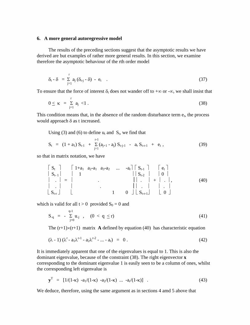
6. A more general autoregressive model

The results of the preceding sections suggest that the asymptotic results we havederived are but examples of rather more general results. In this section, we examinetherefore the asymptotic behaviour of the rth order model

r�t - � = � aj (�t-j - �) - et . (37)

j=1

To ensure that the force of interest �t does not wander off to +� or -�, we shall insist that r0 < � = � aj <1 . (38) j=1

This condition means that, in the absence of the random disturbance term et, the processwould approach � as t increased.

Using (3) and (6) to define ut and St, we find that r-1

St = (1 + a1) St-1 + � (aj+1 - aj) St-j-1 - ar St-r-1 + et , (39) j=1

so that in matrix notation, we have

St � 1+a1 a2-a1 a3-a2 ... -ar� St-1 � et � St- 1 1 � � St-2 � � 0

� . = � . �� . + . , (40) � . � . �� . . �� St-r � � 1 0 � � St-r-1� � 0 �

which is valid for all t > 0 provided S0 = 0 and q-1

S-q = - � u-j , (0 < q < r) (41) j=0

The (r+1)�(r+1) matrix A defined by equation (40) has characteristic equation

(� - 1) (�r - a1�r-1 - a2�r-2 - ... - ar) = 0 . (42)

It is immediately apparent that one of the eigenvalues is equal to 1. This is also thedominant eigenvalue, because of the constraint (38). The right eigenvector xcorresponding to the dominant eigenvalue 1 is easily seen to be a column of ones, whilstthe corresponding left eigenvalue is

yT = [1/(1-�) -a1/(1-�) -a2/(1-�) ... -ar/(1-�)] . (43)

We deduce, therefore, using the same argument as in sections 4 amd 5 above that

r j-1

E(St) � ( � aj � u-i )/(1-�) = ln C; (44)j=1 i=0

Var(St) � t � ; (45)

Cov(St, Su) � min(t, u) � ; (46)

with

� = �2/(1-�) (47)

All the previous approximate annuity and assurance results (11)-(19) follow aspreviously, with � replacing k and C defined by (44).

7. The interest process in the steady state

It is unlikely that an autoregressive model higher than third order will be used toanalyse the interest process. Let us examine therefore the model represented by equation(37) with r=3.

In the steady state, the variance of ut=�-�t will be independent of t, and thecorrelations �1 between ut and ut-1, and �2 between ut and ut-2 will also be independent oft. One can deduce fairly readily by matrix analysis or otherwise that

�1 = (a1+a2a3)/[1-a2-a3(a1+a3)] ; (48)

�2 = a2 + (a1+a3)�1 ; (49)

Var(�t) � �2/[(1-a12-a2

2-a32)-2(a1a2+a2a3)�1-2a1a3�2] . (50)

For the special case of the autoregressive model (1), we observe that

�1 = 2k/(1+k) ; (51)

�2 = k(3k-1)/(1+k) ; (52)

Var(�t) � �2 (1+k)/[(1+3k)(1-k)2] . (53)

The latter result is given in [10]. Using (51)-(53) we can deduce that

Var(�t-�t-1) � 2�2/[(1+3k)(1-k)] . (54)

The corresponding formulae for the first order model (31) are

�1 = k ; (55)

�2 = k2 ; (56)

Var(�t) � �2/(1-k2) ; (57)

Var(�t-�t-1) � 2�2/(1+k) . (58)

Use will be made of some of these results in a later numerical example.

Explicit formulae for processes of higher-order than three are cumbersome. Theasymptotic variance of �t however can be written fairly simply as

�Var(�t) � �2 � bi

2 , (59) i=1

where, with b0 = 1 and bu=0 for u<0,r

bi = � aj bi-j . (60) j=1

8. Accumulations

So far, we have considered only discounted values. For some purposes (e.g.maturity guarantees), accumulations are more relevant. We start with the relationship

(1+it+1)(1+it+2)...(1+in) = (1+i)n-t exp(St-Sn) , (61)

in which it is the interest rate experienced in year t and i is the interest rate correspondingto the assumed long-term central force of interest �. In the general case of section 6, wecan deduce for large t and n that

E[(1+it+1)...(1+in) � (1 + i)n-t exp[(n-t)�/2] ; (62)

E[(1+it+1)...(1+in)]2 � (1 + i)2(n-t) exp[(n-t)�] ; (63)

E[(1+it+1)...(1+in)][(1+iu+1)...(1+in)]

� (1+i)n-t(1+i)n-u exp[(n-t)�/2 + (n-u)�/2 + min(n-t,n-u)�] . (64)

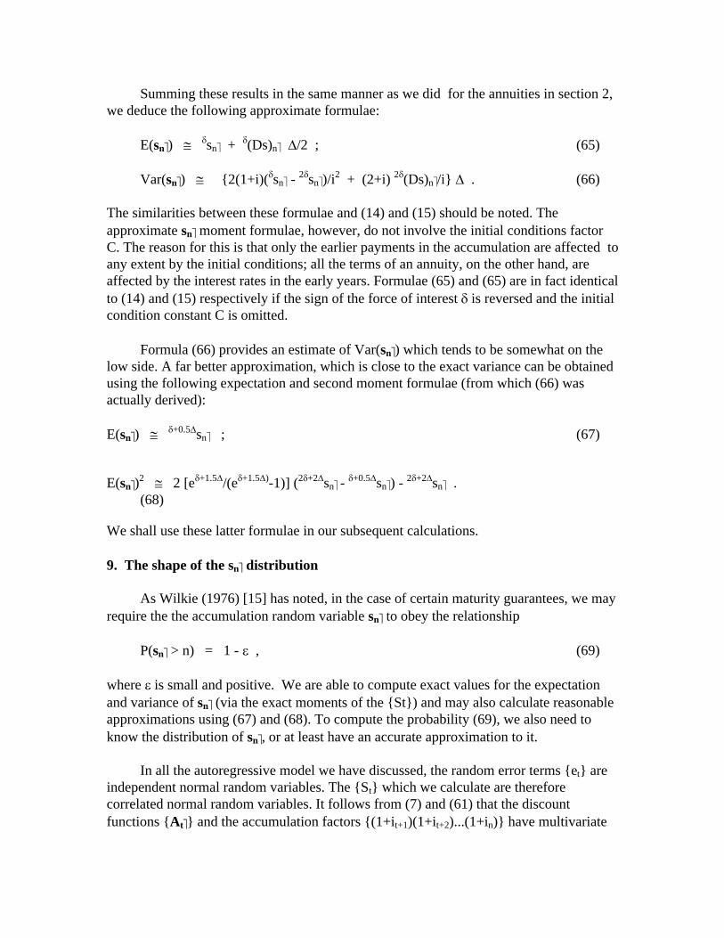
Summing these results in the same manner as we did for the annuities in section 2,we deduce the following approximate formulae:

E(sn�) � �sn� + �(Ds)n� �/2 ; (65)

Var(sn�) � {2(1+i)(�sn� - 2�sn�)/i

2 + (2+i) 2�(Ds)n�/i} � . (66)

The similarities between these formulae and (14) and (15) should be noted. Theapproximate sn� moment formulae, however, do not involve the initial conditions factorC. The reason for this is that only the earlier payments in the accumulation are affected toany extent by the initial conditions; all the terms of an annuity, on the other hand, areaffected by the interest rates in the early years. Formulae (65) and (65) are in fact identicalto (14) and (15) respectively if the sign of the force of interest � is reversed and the initialcondition constant C is omitted.

Formula (66) provides an estimate of Var(sn�) which tends to be somewhat on thelow side. A far better approximation, which is close to the exact variance can be obtainedusing the following expectation and second moment formulae (from which (66) wasactually derived):

E(sn�) � �+0.5�sn� ; (67)

E(sn�)2 � 2 [e�+1.5�/(e�+1.5�)-1)] (2�+2�sn� -

�+0.5�sn�) - 2�+2�sn� .

(68)

We shall use these latter formulae in our subsequent calculations.

9. The shape of the sn� distribution

As Wilkie (1976) [15] has noted, in the case of certain maturity guarantees, we mayrequire the the accumulation random variable sn� to obey the relationship

P(sn� > n) = 1 - � , (69)

where � is small and positive. We are able to compute exact values for the expectationand variance of sn� (via the exact moments of the {St}) and may also calculate reasonableapproximations using (67) and (68). To compute the probability (69), we also need toknow the distribution of sn�, or at least have an accurate approximation to it.

In all the autoregressive model we have discussed, the random error terms {et} areindependent normal random variables. The {St} which we calculate are thereforecorrelated normal random variables. It follows from (7) and (61) that the discountfunctions {At�} and the accumulation factors {(1+it+1)(1+it+2)...(1+in)} have multivariate

lognormal distributions. Knowing the expectations and second-order moments of thesevariables, we can therefore make exact probabilistic statements about them.

The random variables at� and sn-t� are more problemmatic, as each comprises thesum of a series of random variables which have the multivariate lognormal distribution.Given their structure, both these random variables can be expected to retain some of theskewness inherent in their individual correlated lognormal terms. The use of thelognormal distribution would seem a plausible approximation for the distribution ofeach.

As a check on this proposed approximation, 1,000 simulations of the second-orderautoregressive process (1) were performed, with parameters k=0.5, �=0.05, �=ln(1.15),and �-1=�0=�. The resulting cumulative distribution of the s10� distribution is shown ascolumn (2) in table 4. The simulated distribution has mean 24.412 and variance 36.775.

If exact theoretical calculations of the s10� moments are performed, a mean of24.051 and variance of 33.686 emerge. The lognormal distribution having these momentsis shown in column (3) of table 4. A Kolmogorov-Smirnov test indicates no significantdifference between the simulated distribution and the theoretical lognormal distribution.

The interest process used in this simulation study has parameters which allow quitelarge and rapid changes in the interest rate (figure 1). Yet the lognormal distributionprovided an accurate approximation to the unknown distribution of s10�. It would seemappropriate therefore to use either the lognormal distribution with exactly calculatedmoments, or the lognormal distribution with the approximate moments (67) and (68) toapproximate the unknown theoretical distribution of sn� in the more general situation.

We would also expect the lognormal to provide an accurate approximation to thedistribution of at� in the same way.

10. A numerical example

An insurance company markets an investment product under which annualpremiums of $1 are payable for 10 years. At the end of the 10-year period, the insured isentitled to 97.5% of the accumulated premiums. There is a guarantee that the amount paidto the policyholder will be no less than the full premiums accumulated at 7.5% perannum.

In recent years, the earnings rate of the fund has been in the neighbourhood of 15%per annum, and the company believes that future earnings should vary around this level.The earnings of the fund in any given future year are expected to lie in the range 0% tp30% with a high probability, and a change in investment return from one year to the nextof more than 12 percentage points is considered most unlikely.

What is the probability that the insurer will receive less than 2.5% of theaccumulated fund? Find also the insurer’s expected income from one such policy.

The accumulation of ten $1 annual premiums at 7.5% is .075s10�=15.2081. If 97.5%of the accumulated premiums is less than this amount, the insurer will have to meet thematurity guarantee that it has given, and its income from the policy will be less than 2.5%of the accumulated value. We require therefore

P(0.975 s10� < 15.2081)

i.e. the probability that the random accumulation function s10� is less than15.2081/0.975=15.598.

Let us adopt the second-order autoregressive model (1) for demonstration purposes,and assume a long-term central investment force of return �=ln(1.15)=0.13976. If thereturn in any given future year is to lie in the range 0% to 30% with a high probability,then (with a 95% confidence level in mind) the standard error of any �t in the futureshould be about 0.08. Using similar reasoning, if a change in investment return from oneyear to the next of more than 12 percentage points is unlikely, then the standard deviationof �t-�t-1 must be about 0.065.

To obtain the parameters �2 and k of the autoregressive process, we equate (53) tothe square of 0.08 and (54) to the square of 0.065, yielding �=0.0513 and k=0.5037. Ourcalculations below will be based on �=0.05 and k=0.5, which correspond to standarddeviations of 0.0775 and 0.0632 for �t and �t-�t-1 respectively for a given year well in thefuture. With these parameters, (67) and (68) indicate an expected value of 24.122 for s10�

and a variance of 30.775. Using a lognormal approximation for the distribution of s10�, wededuce that the probability that the insurer will receive less than 2.5% of theaccumulation is about 0.035 and the expected income to the insurer from such a policy is$0.57.

11. Inflation and investment earnings

The actuary advising a defined benefit pension scheme will be very interested infuture inflation rates, market rates of investment return and the return that will beachieved on the investments of the fund. These three rates are not unrelated. Higher ratesof inflation, for example will tend to induce higher market rates of return, which in turnwill impinge on the return obtained by the fund.

The matrix methods of sections 4, 5 and 6 are readily adapted to the analysis ofsimultaneous autoregressive models in which the fluctuating forces of inflation, marketinvestment return and fund return are related, providing asymptotic formulae for themoments and useful approximations. The model we describe below is solely fordemonstration purposes.

Let us define xt to be the force of inflation during the year to time t, and postulate acentral force of inflation � about which the inflation rate will vary, and assume fordemonstration purposes that

xt - � = 2 k (xt-1 - �) - k (xt-2 -�) + et . (70)

As before, we assume that 0 < k <1. The random error term et is normally distributed withzero mean and variance �x

2, and the {et} are mutually independent.

If we argue that the force of market return yt in year t is influenced partly by its ownrecent history and by inflationary trends, a possible model for the deviation of the marketrate of return from its assumed long term central value � is a combination of its previouslevel and the expected deviation of inflation from its long term central value:

yt - � = b (yt-1 - �) + c [2 k(xt-1 - �) - k(xt-2 - �)] + ft , (71)

where b and c are constants (0 < c < 1), and the {ft} are mutually independent randomerror terms with zero means and constant variances �y

2, which are also independent of the{et}.

The force of return on the fund will be influenced by its existing investments aswell as the market, and for demonstration purposes we shall assume that the deviation ofthe fund return zt in year t from its postulated long term central level � is influenced byboth its previous level and the expected level of the market:

zt - � = d (zt-1 -�) + (1-d) [c(yt-1 - �) + 2kb(xt-1 - �) - kb(xt-2 - �)] + gt . (72)

The constant d is constrained so that 0 < d < 1, and the random error terms {gt} areindependent normal random variables with zero means and variances �z

2, independent ofthe {et} and {ft}.

In section 4, we replaced ut = �-�t by the difference St-St-1 of the cumulative sum St,

and obtained a matrix equation for the {St}. Let us now define Xt, Yt and Zt to be thecumulative sums of xt-�, yt-� and zt-� respectively, and proceed in the same manner. Wefind that the vector of cumulative sums wt, defined by

wtT = (Xt Xt-1 Xt-2 Yt Yt-1 Zt Zt-1) (73)

obeys the matrix recurrence equation

wt = A wt-1 + �t , (74)

where �t is a column vector with et as its first element, ft as its fourth element, gt as itssixth element, and zeros elsewhere, and

1+2k -3k k 0 0 0 0 � 1 0 0 0 0 0 0 �

0 1 0 0 0 0 0 � ___________________________________________ �

A = 2kb -3kb kb 1+c -c 0 0 � . (75) 0 0 0 1 0 0 0 � ___________________________________________ � 2k(1-d)b -3k(1-d)b k(1-d)b (1-d)c -(1-d)c 1+d -d � � 0 0 0 0 0 1 0 �

Because of the block structure of A, its eigenvalues are those of the three principalsubmatrices, each of which has a dominant eigenvalue of 1. The seven eigenvalues are infact 1, 1, 1, k+�[k(1-k)], c and d. Denoting the dominant right and left eigenvextors of thethree principal submatrices of A by x and !x

T, y and !yT, z and !z

T respectively, wenote that At approaches

x !xT 0 0 �

A� = Byx y !yT 0 � . (76)

� Bzx Bzy z!zT �

A little algebra reveals that the submatrices Byx, Bzx and Bzy take the forms y"xT , z"x

T

and z"yT respectively, where

"xT = (L -2L L) ; (77)

"yT = (M -M) ; (78)

withL = k b / [(1-c)(1-k)] ; (79)

M = c / (1-c) . (80)

Using these results and the same methods as in section 4, we deduce that for large t

E(Xt) � k(x0 - x-1)/(1-k) ; (81)

E(Yt) � L(x0 - x-1) + c(y0 - �)/(1-c) ; (82)

E(Zt) � L(x0 - x-1) + M(y0 -�) + d(z0 - �)/(1-d) ; (83)

Var(Xt) � t �x2/(1-k)2 ; (84)

Var(Yt) � t [�y2/(1-c)2 + L2�x

2] ; (85)

Var(Zt) � t[�z2/(1-d)2 + L2�x

2 + M2�y2] ; (86)

Cov(Xt, Yt) � t L �x2/(1-k) ; (87)

Cov(Xt, Zt) � t L �x2/(1-k) ; (88)

Cov(Yt, Zt) � t [L2 �x2 + M �y

2/(1-c)] . (89)

The forms of the variances and covariances are not without interest. If, for example,�y

2 = �z2 = 0, the random variables Xt and Zt are asymptotically fully correlated. Other

relationships are also evident.

Under this model, the present value at the earnings rate of the fund of a lump sum,currently 1, but adjusted for inflation, is the lognormal random variable exp(Xt - Zt).The moments are readily approximated using the asymptotic moments for Xt and Zt andthe approximate formulae we derived for the earlier models.

12. Concluding remarks

Varying levels of inflation and fluctuating investment returns are problems withwhich the actuary must contend on an almost daily basis. Unlike mortality and otherdecrements or movements, for which deterministic and stochastic models are readilyavailable, these economic factors are rather more difficult to model. Autoregressivemethods are attractive for this purpose and have been proposed by a variety of authors.Many of the formulae which emerge from the autoregressive modelling of these processesare rather complicated. A major objective of this paper has been to show that practicalapproximate formulae are available in many instances, that these formulae do provideadequate approximations, and that day-to-day problems can be tackled using them.

13. References

[1] Boyle, P.P. (1976) Rates of return as random variables. J. Risk and Insurance, 43,693-713.

[2] Dufresne, D. (1988) Moments of pension fund contributions and fund levels when rates of return are random. J Institute of Actuaries, 115, 535-544.

[3] Giaccotto, C. (1986) Stochastic modelling of interest rates: actuarial vs. equilibriumapproach. J. Risk and Insurance, 53, 435-453.

[4] Haberman, S. (1993) Pension funding with time delays and autoregressive rates of return. Insurance: Mathematics and Economics, 13, 45-56.

[5] Haberman, S. (1994) Autoregressive rates of return and the variability of pension contributions and funds levels for a defined benefit pension scheme. Insurance: Mathematics and Economics, 14, 219-240.

[6] Panjer, H.H. and Bellhouse, D.R. (1980) Stochastic modelling of interest rates with applications to life contingencies. J. Risk and Insurance, 47, 91-110.

[7] Panjer, H.H.`and Bellhouse, D.R. (1981) Stochastic modelling of interest rates with applications to life contingencies - Part II. J. Risk and Insurance, 48, 628-637.

[8] Parzen, E. (1962) Stochastic Processes. Holden-Day, San Francisco.[9] Pollard, A.H. and Pollard, J.H. (1969) A stochastic approach to actuarial functions.

J. Institute of Actuaries, 95, 79-113.[10] Pollard, J.H. (1971) On fluctuating interest rates. Bulletin de l’Association Royale

des Actuairs Belges, 66, 68-97.[11] Pollard, J.H. (1973) Mathematical Models for the Growth of Human

Populations, 44. Cambridge University Press.[12] Pollard, J.H. (1976) Premium loadings for non-participating business. J. Institute

of Actuaries, 103, 205-212.[13] Scott, W.F. (1977) A reserve basis for maturity guarantees in unit-linked life

assurance. Transactions of the Faculty of Actuaries, 35, 365-385.[14] Westcott, D.A. (1981) Moments of compound interest functions under fluctuating

interest rates. Scandinavian Actuarial Journal, (1981 volume), 237-244.[15] Wilkie, A.D. (1976) The rate of interest as a stochastic process. Theory and

applications. Proceedings of the 20th International Congress of Actuaries, 1, 325-338.

Table 2Assurance and annuity certain expectations: exact and approximate values for the

second-order model (1) with �=ln(1.05), �=0.001 and k=0.9.

________________________________________________________________________Term Assurance Annuity

______________________ ____________________________ n Exact Approx Exact Approx________________________________________________________________________

Case i-1=0.05, i0=0.05

20 0.3773 0.3773 12.469 12.473 30 0.2318 0.2317 15.383 15.391 40 0.1424 0.1423 17.173 17.184 60 0.0537 0.0537 18.948 18.963 80 0.0203 0.0203 19.618 19.634

Case i-1=0.06, i0=0.07

20 0.3559 0.3467 11.374 11.463 30 0.2100 0.2130 14.025 14.144 40 0.1318 0.1308 15.681 15.791 60 0.0495 0.0493 17.309 17.426 80 0.0186 0.0186 17.924 18.043

Case i-1=0.07, i0=0.06

20 0.3982 0.4105 13.470 13.573 30 0.2569 0.2521 16.627 16.748 40 0.1532 0.1549 18.579 18.699 60 0.0582 0.0584 20.510 20.635 80 0.0220 0.0220 21.239 21.366________________________________________________________________________

Table 1Assurances and annuities certain: exact and approximate second moments for the

second order model (1) with �=ln(1.05), �=0.001 and k=0.9.

________________________________________________________________________Term Assurance Variance Assurance/annuity covariance Annuity variance

� 104 � 103

________________ ________________________ ____________________Exact Approx. Exact Approx. Exact Approx.

________________________________________________________________________

Case i-1=0.05,i0=0.05

20 3.358 2.844 3.8579 4.1816 0.0848 0.0882 30 1.856 1.608 4.2115 4.2572 0.1619 0.1727 40 0.896 0.809 3.3802 3.5043 0.2378 0.2491 60 0.186 0.172 1.7456 1.7842 0.3369 0.3508 80 0.035 0.033 0.7534 0.7652 0.3834 0.3982

Case i-1=0.06, i0=0.07

20 2.988 2.402 3.3686 3.5314 0.0706 0.0745 30 1.523 1.359 3.4805 3.5952 0.1349 0.1458 40 0.768 0.683 2.8774 2.9594 0.1993 0.2104 60 0.158 0.146 1.4760 1.5067 0.2827 0.2962 80 0.029 0.028 0.6358 0.6462 0.3220 0.3362

Case i-1=0.7, i0=0.06

20 3.740 3.367 4.4614 4.9516 0.1034 0.1045 30 2.279 1.905 5.1140 5.0412 0.1948 0.2045 40 1.038 0.958 3.9720 4.1496 0.2854 0.2950 60 0.219 0.204 2.0649 2.1127 0.4031 0.4154 80 0.041 0.039 0.8932 0.9061 0.4584 0.4715________________________________________________________________________

Table 3 Life annuity variance, and components due to interest rate variation

and variation in age at deatha

________________________________________________________________________Age Exact variance of ax Approx. variance of ax Age at death Varying interest x (age at death and (equation (19)) component component

interest both varying) of (3) of (3)

(1) (2) (3) (4) (5)________________________________________________________________________ 20 4.779 4.851 4.472 0.379 30 6.015 6.074 5.753 0.321 40 9.398 9.438 9.190 0.248 50 14.122 14.142 13.974 0.167 60 16.392 16.398 16.304 0.095________________________________________________________________________aIn this example, �=0.01, k=0.9, i=0.05, i-1=i0=0.05.

Table 4Cumulative distribution of s10�

________________________________________________________________________P(s10� < x) P(s10� < x) P(s10� < x)

x _____________ x __________________ x _______________Simul- Log- Simul- Log- Simul- Log-ation normal ation normal ation normal

(1) (2) (3) (1) (2) (3) (1) (2) (3)________________________________________________________________________10.5 .000 .001 27.5 .778 .776 44.5 .990 .99711.5 .002 .003 28.5 .815 .818 45.5 .994 .99812.5 .004 .007 29.5 .840 .853 46.5 .995 .99913.5 .013 .016 30.5 .866 .882 47.5 .998 .99914.5 .023 .031 31.5 .890 .906 48.5 .998 .99915.5 .037 .055 32.5 .915 .926 49.5 .998 .99916.5 .071 .090 33.5 .930 .942 50.5 .998 1.00017.5 .109 .136 34.5 .947 .955 51.5 .999 1.00018.5 .167 .192 35.5 .958 .965 52.5 .999 1.00019.5 .246 .256 36.5 .963 .973 53.5 .999 1.00020.5 .304 .326 37.5 .970 .979 54.5 .999 1.00021.5 .387 .399 38.5 .976 .984 55.5 .999 1.00022.5 .461 .473 39.5 .980 .988 56.5 .999 1.00023.5 .539 .544 40.5 .982 .991 57.5 .999 1.00024.5 .601 .611 41.5 .983 .993 58.5 1.000 1.00025.5 .664 .673 42.5 .987 .995 59.5 1.000 1.00026.5 .719 .728 43.5 .989 .996 60.5 1.000 1.000________________________________________________________________________

Figure 1Three independent simulations of the interest rate trajectory under the second-

order autoregressive model (1) with i=0.15, �=0.05, k=0.5, and i-1=i0=0.15.

-0.1

0

0.1

0.2

0.3

0.4

0.5

0 1 2 3 4 5 6 7 8 9 10

time t

inte

rest

rat

e