Anchors Away: How Fiscal Policy Can Undermine the Taylor ... · Anchors Away: How Fiscal Policy Can...

NBER WORKING PAPER SERIES

ANCHORS AWAY: HOW FISCAL POLICY CAN UNDERMINE THE TAYLORPRINCIPLE

Eric M. Leeper

Working Paper 15514http://www.nber.org/papers/w15514

NATIONAL BUREAU OF ECONOMIC RESEARCH1050 Massachusetts Avenue

Cambridge, MA 02138November 2009

Prepared for the Banco Central de Chile's 13th Annual Conference, November 19 and 20, 2009. I thankTodd Walker for many insightful conversations. The views expressed herein are those of the author(s)and do not necessarily reflect the views of the National Bureau of Economic Research.

NBER working papers are circulated for discussion and comment purposes. They have not been peer-reviewed or been subject to the review by the NBER Board of Directors that accompanies officialNBER publications.

© 2009 by Eric M. Leeper. All rights reserved. Short sections of text, not to exceed two paragraphs,may be quoted without explicit permission provided that full credit, including © notice, is given tothe source.

Anchors Away: How Fiscal Policy Can Undermine the Taylor PrincipleEric M. LeeperNBER Working Paper No. 15514November 2009JEL No. E31,E52,E62

ABSTRACT

Slow moving demographics are aging populations around the world and pushing many countries intoan extended period of heightened fiscal stress. In some countries, taxes alone cannot or likely willnot fully fund projected pension and health care expenditures. If economic agents place sufficient probabilityon the economy hitting its "fiscal limit" at some point in the future--after which further tax revenuesare not forthcoming--it may no longer be possible for monetary policy behavior that obeys the Taylorprinciple to control inflation or anchor inflation expectations. In the period leading up to the fiscallimit, the more aggressively that monetary policy leans against inflationary winds, the more expectedinflation becomes unhinged from the inflation target. Problems confronting monetary policy are exacerbatedwhen policy institutions leave fiscal objectives and targets unspecified and, therefore, fiscal expectationsunanchored. In light of this theory, the paper contrasts monetary-fiscal policy frameworks in the UnitedStates and Chile.

Eric M. LeeperDepartment of Economics304 Wylie HallIndiana UniversityBloomington, IN 47405and [email protected]

Anchors Away: How Fiscal Policy

Can Undermine the Taylor Principle∗

Eric M. Leeper†

November 9, 2009

1 Introduction

Policymakers have long understood that if fiscal policy runs amuck and monetary policyis forced to raise seigniorage revenues, big inflations result. Latin American policymakersunderstand this outcome better than most. This message is implicit in Cagan’s (1956)initial study of hyperinflation and the message is explicit in Sargent and Wallace’s (1981)theoretical analysis of how monetary policy can lose control of inflation and Sargent’s (1983)interpretation of historical episodes of high inflations. The message is forcefully promulgatedby international economic organizations that prescribe policy reforms to troubled economies.Underlying this view is the notion that if central bankers display sufficient resolve and stickto their inflation-fighting guns, fiscal policy will eventually relent and reform. Unfortunately,wishing it were so does not make it so.

Recent research on monetary and fiscal policies has learned that the ways in which policiesinteract to determine inflation and influence the real economy are far more subtle than the“monetization of debt” perspective implies. For example, Sargent and Wallace’s (1975) earlyfinding that if the central bank pegs the nominal interest rate—or more generally does notadjust the rate strongly with inflation—then the equilibrium inflation rate is undetermined,is not robust to alternative assumptions about fiscal behavior: Leeper (1991) and othershave shown that if primary surpluses are unresponsive to the state of government debt, theninflation is uniquely determined. This is not merely of academic interest. Central banksdo go through periods when they adjust interest rates weakly to inflation and many banksare now, in effect, pegging the nominal rate near the zero lower bound. If such behaviorendangered price stability by not pinning down the inflation process, this would be of greatpractical concern.

Another example that has received much attention is that when a government issuesnominal debt denominated in its home currency, it is possible for fluctuations in current or

∗November 9, 2009. Prepared for the Banco Central de Chile’s 13th Annual Conference, November 19and 20, 2009. I thank Todd Walker for many insightful conversations.

†Indiana University and NBER, [email protected].

How Fiscal Policy Can Undermine the Taylor Principle

expected primary surpluses to generate important aggregate demand effects.1 Policies thatset the nominal interest rate independently of inflation and primary surpluses independentlyof outstanding debt represent the canonical case in which a debt-financed tax cut today,which does not carry with it an expectation of higher taxes in the future, raises householdwealth and increases aggregate demand. In the standard models used for policy analysis,higher demand raises both output and inflation; higher inflation serves to revalue outstandingnominal debt. Debt revaluation can be an important source of fiscal financing by ensuringthat this mix of policies is sustainable.

This canonical case also points to circumstances in which monetary policy can no longercontrol inflation. Some observers dismiss the case as special, preferring to stick to theconvention that fiscal policy is Ricardian in the sense that expansions in debt are alwaysbacked by higher expected primary surpluses [McCallum (2001)]. Unfortunately, as I shallargue, demographic, political, and economics realities in many countries may not conformto this conventional view.

Within the class of new Keynesian models now in wide use for monetary policy analysis,something of a consensus has developed around what constitutes “good” monetary policybehavior. In terms of implementable simple rules—as opposed to, say, Ramsey optimalsolutions—a necessary condition is that the central bank adjust the nominal interest ratemore than one-for-one with inflation; this is called the “Taylor principle” [Taylor (1993)].This principle seems to produce nearly optimal outcomes in models now in use at centralbanks [see, for example, Henderson and McKibbin (1993), Rotemberg and Woodford (1997,1999), Schmitt-Grohe and Uribe (2007), and papers in Taylor (1999b)].

In this paper I explore how the Taylor principle characterization of “good” monetarypolicy fares in periods of heightened fiscal stress. Fiscal stress is what Chile, the UnitedStates, much of Europe, Japan, and a great many other countries are facing in the comingdecades as their populations age and government transfer payments for pensions and healthcare are anticipated to rise substantially as a share of GDP.

It is unlikely that tax revenues alone can finance these promised transfers. Some coun-tries are already at or near the peaks of their Laffer curves, according to some estimates[Trabandt and Uhlig (2009)]. In those countries, it may be economically impossible to raisesufficient revenues. Other countries—with the United States as the leading example—seemto have little tolerance for high tax rates and may find it politically impossible to raise taxesenough. In either scenario, these countries could easily reach their fiscal limits well before the“generational storm”—in Kotlikoff and Burns’s (2004) memorable phrase—has fully playedout. At its fiscal limit, a government can no longer follow the conventional prescription bywhich fiscal policy takes care of itself—and everything else that affects the value of govern-ment debt—by financing government debt entirely through future surpluses. By extension,the fiscal limit makes it infeasible for monetary policy to always obey the Taylor principle,for doing so results in unsustainable policies.

At the fiscal limit, macro policies enter a new realm that economists have only begunto study systematically. Once taxes can no longer adjust and government purchases haveachieved their socially acceptable lower bound, only two sources of fiscal financing remain:

1The list of contributors to this literature is long, but some key papers include Leeper (1991, 1993),Woodford (1994, 1995), Sims (1994, 2005), Cochrane (1999, 2001), Leith and Wren-Lewis (2000), Schmitt-Grohe and Uribe (2000), Daniel (2001), and Corsetti and Mackowiak (2006).

2


incomplete honoring of promised transfers and surprise revaluations of outstanding nominalgovernment bonds or some combination of both.2 The first option would permit monetarypolicy to continue to follow a Taylor principle because, in effect, actual transfers are adjust-ing to finance government debt. But the same demographics that are behind the growingtransfers payments also create powerful political pressures for democratic governments tohonor their earlier promises. The second option allows the government to fully honor itsfinancial commitments, but requires the central bank to give up control of inflation. A morelikely outcome is some mix of the two options, possibly with policy fluctuating betweenthe two distinct monetary-fiscal regimes. With the mixed outcome, monetary policy wouldstill lose control of inflation, as Davig and Leeper (2006b, 2009), Chung, Davig, and Leeper(2007), and Davig, Leeper, and Walker (2009) show.

No government has made it completely clear to its populace how the coming fiscal stormwill be weathered. Existing rules governing fiscal behavior, where they exist, are not obvi-ously robust to an environment in which government transfers constitute a growing fractionof GDP. And how such fiscal rules interact with, say, an inflation-targeting monetary policyis not well understood. Some large countries, like Germany, the United Kingdom, and theUnited States, seem to have made no provisions whatsoever for dealing with future fiscalstresses. In those countries, the public has no choice but to speculate about how futurepolicies will adjust. How can expectations of inflation and interest rates be anchored bymonetary policy in this new policy realm? What will determine such expectations if notmonetary policy? How does the public’s speculation about future policy adjustments affectthe equilibrium today?

1.1 Anchoring Expectations There is much ballyhoo about how a major benefit ofhaving central banks adopt an explicit inflation target is that it contributes in important waysto anchoring private expectations of inflation. There are as many definitions of “anchoringexpectations” as there are people repeating the mantra. Faust and Henderson (2004) grapplewith the definition in their thoughtful piece about best-practice monetary policy. Manyof their concerns spring from the fact that central banks—even inflation targeters—havemultiple objectives and face tradeoffs among those objectives. For our purposes, we simplifythe problem by positing that the central bank targets only inflation at π∗ and the taxauthority targets only government debt at b∗. Faust and Henderson correctly observe thatif the primary objective of inflation targeting is to anchor long-run expectations of inflation,then formally this amounts to ensuring that limj→∞ Etπt+j = π∗. But by this definitionof anchoring, as Faust and Henderson point out, best-practice monetary policy permits|Etπt+j − π∗| > ε > 0 for all j ≥ 0: at times, expected inflation over any forecast horizonwill be very far from target.

No inflation-targeting central bank embraces such a liberal definition of anchoring expec-tations. The Central Bank of Chile aims “to keep annual CPI inflation around 3% most ofthe time” [Banco Central de Chile (2007)]. Sveriges Riksbank targets 2 percent in Sweden

2I take off the table two other options: sovereign debt default and pure inflation taxes. It is difficultto imagine an equilibrium in which many large countries default simultaneously, though this possibilitydeserves further research. Pure inflation taxes are removed on the grounds that historical experience withhyperinflations has found them to be an extraordinarily costly means of fiscal financing. Moreover, likeincome taxes, inflation taxes are also subject to a Laffer curve and, therefore, a fiscal limit.

3


[Sveriges Riksbank (2008)]. Both Chile and Sweden have a tolerance range of plus or minus1 percentage point. In New Zealand, the Reserve Bank targets CPI inflation between 1 and3 percent [Reserve Bank of New Zealand (2008)]. It is not apparent from their web pages,but I imagine that all inflation-targeting central banks would interpret “long run” to besomething shy of infinity. I also imagine that if in those economies expected inflation coulddrift arbitrarily far from target for arbitrarily long periods, the central banks would notfeel that they have successfully anchored long-run inflation expectations (even if one couldprove that the Faust-Henderson limiting condition for expected inflation held). Analogousranges tend to be applied in ministries of finance and treasuries that have an explicit targetfor government debt [see, for example, New Zealand Treasury (2009), Swedish Ministry ofFinance (2008)].

In this paper I shall adopt the more pragmatic notion of anchored expectations that policyauthorities seem to apply. If in an equilibrium, expectations of a policy target variable candeviate widely from target for an extended period, then expectations are not well anchoredon the announced targets.

1.2 What the Theory Says I lay out three very simple theoretical models to makeconcrete the issues that arise in an environment where taxes have reached their limit, butgovernment transfers grow relentlessly. The theory suggests that even if economic agentsknow how policies will adjust once the economy hits the fiscal limit, it may no longer bepossible for monetary policy to achieve its inflation target.3 Monetary policy’s loss of controlof inflation begins well before the fiscal limit is hit. Because agents know such a limit exists,monetary policy cannot control inflation even in the period leading up to the limit whenmonetary policy dutifully follows the Taylor principle and fiscal policy systematically raisestaxes to stabilize debt.

The central bank’s problems controlling inflation become more profound in the arguablymore plausible environment where agents are uncertain about how monetary and fiscal poli-cies will adjust in the future once the fiscal limit is reached. In such a setting it is easy tosee how expectations can become unanchored, particularly if monetary and fiscal authoritiesdo little to help resolve uncertainty about future policies.

Policy uncertainty almost certainly reduces welfare. Existing work tends to model theuncertainty in rather stylized forms—a stochastic capital tax, for example—but nonethelessfinds that greater uncertainty reduces growth and welfare [Hopenhayn (1996) and Aizenmanand Marion (1993)]. Uncertainty can also generate an option value for waiting to invest-ment, which slows growth [Bernanke (1983), Dixit (1989), and Pindyck (1988)]. Indeed, oneargument for having central banks announce their intended interest rate paths is to reduceuncertainty about monetary policy and better anchor expectations and improve the effec-tiveness of monetary policy [Faust and Leeper (2005), Rudebusch and Williams (2006), andSvensson (2006)]. While the implications of uncertainty for welfare are important, I do notpursue them in the positive analysis that follows.

3Sims (2005) makes closely related points in the context of inflation targeting. Sims (2009) explainsthat as an application of Wallace’s (1981) Modigliani-Miller theorem for open-market operations, many ofthe extraordinary measures that central banks have taken over the past year or so run the risk of beinginsufficiently backed by fiscal policy and, therefore, may make it difficult for monetary policy alone to anchorinflation.

4


In light of the profound policy uncertainty that many countries will soon face, I findmyself in sympathy with North (1990, p. 83): “The major role of institutions in a societyis to reduce uncertainty by establishing a stable (but not necessarily efficient) structureto human interaction. The overall stability of an institutional framework makes complexexchange possible across both time and space.” Only the policy institutions themselves—via the desires of the electorate—can help to resolve the uncertainty and only by reducinguncertainty can policy institutions hope to anchor expectations reliably.

After deriving theoretical results, the paper turns to contrast the monetary-fiscal policyframeworks in Chile and the United States. Whereas Chile has adopted specific objectivesand even rules for the conduct of monetary and fiscal policy, America has consistently es-chewed rules-based policies. Chile’s policies contribute toward keeping the economy wellaway from the fiscal limit, permitting Banco Central de Chile to target inflation and anchorexpectations of inflation. In contrast, in the United States, agents have good reason to beconcerned that taxes may reach the fiscal limit, undermining the Federal Reserve’s abilityto control inflation now and in the future.

2 Three Simple Models

I present three models of price-level and inflation determination that increase in the subtletyof the interactions between monetary and fiscal policies. Throughout the analysis I restrictattention to rational expectations equilibria, so the results I present can be readily contrastedto prevailing views, which also are based on rational expectations.

The first model draws from Leeper (1991), Sims (1994), and Woodford (2001) to lay thegroundwork for how monetary and fiscal policies jointly determine equilibrium. These resultsare well known, but the broader implications of thinking about macro policies jointly are notfully appreciated. A second model adds one layer of subtlety by positing that at some knowndate in the future, call it T , the economy will reach its fiscal limit, at which point it is notpossible to raise further revenues. At that limit, policy regime—the mix of monetary andfiscal rules—changes in some known way. This model illustrates how expectations of futurepolicies can feed back to affect the current equilibrium. The final model adds one more layerof subtlety: although agents know regime will change at date T , they are uncertain whatmix of monetary and fiscal policies will be realized. In the third model, agents’ expectationsof inflation depend on the subjective probabilities they attach to possible future policies.The last two models draw on work in Davig, Leeper, and Walker (2009).

The models illustrate how interactions between monetary and fiscal policies, the possi-bility of regime changes, and uncertainty about future regimes create difficulties for policyauthorities who aim to anchor private expectations on the targets of policy.

Each model has a common specification of the behavior of the private sector. An infinitelylived representative household is endowed each period with a constant quantity of non-storable goods, y. To keep the focus away from seigniorage considerations, we examine acashless economy, which can be obtained by making the role of fiat currency infinitesimallysmall. Government issues nominal one-period bonds, allowing us to define the price level,P , as the rate at which bonds exchange for goods.

5


The household chooses sequences of consumption and bonds, {ct, Bt}, to maximize

E0

∞∑

t=0

βtu(ct), 0 < β < 1 (1)

subject to the budget constraint

ct +Bt

Pt

+ τt = y + zt +Rt−1Bt−1

Pt

(2)

taking prices and R−1B−1 > 0 as given. The household pays taxes, τt, and receives transfers,zt, each period, both of which are lump sum.

Government spending is zero each period, so the government chooses sequences of taxes,transfers, and debt to satisfy its flow constraint

Bt

Pt

+ τt = zt +Rt−1Bt−1

Pt

(3)

given R−1B−1 > 0, while the monetary authority chooses a sequence for the nominal interestrate.

After imposing goods market clearing, ct = y for t ≥ 0, the household’s consumptionEuler equation reduces to the simple Fisher relation

1

Rt

= βEt

(

Pt

Pt+1

)

(4)

The exogenous (fixed) gross real interest rate, 1/β, makes the analysis easier but is notwithout some lose of generality, as Davig, Leeper, and Walker (2009) show in the contextof fiscal financing in a model with nominal rigidities. This is less the case in a small openeconomy, so one interpretation of this model is that it is a small open economy in whichgovernment debt is denominated in terms of the home nominal bonds (“currency”) and alldebt is held by domestic agents.

2.1 Model 1 I begin with simple fixed policy regimes in order to solidify the understand-ing of how monetary and fiscal policies jointly determine the equilibrium price level andinflation rate. The focus on price-level determination is entirely for analytical convenience;it is not a statement that inflation is the only thing macro policy authority do or should careabout. Because price-level determination is the first step toward understanding how macropolicies affect the aggregate economies, the key insights I derive from this model extend tomore complex environments.

2.1.1 Active Monetary/Passive Tax Policy This model reiterates well-known re-sults about how inflation is determined in the canonical model of monetary policy, as pre-sented in textbooks by Galı (2008) and Woodford (2003), for example. This regime—denotedactive monetary and passive fiscal policy—combines an interest rate rule in which the centralbank aggressively adjusts the nominal rate in response to current inflation with a tax rule inwhich the tax authority adjusts taxes in response to government debt sufficiently to stabilize

6


debt.4 In this textbook, best-of-all-possible worlds, monetary policy can consistently hit itsinflation target and fiscal policy can achieve its target for the real value of debt.

To derive the equilibrium price level for the model laid out above, we need to specify rulesfor monetary, tax, and transfers policies. Monetary policy follows a conventional interest raterule, which for analytical convenience, is written somewhat unconventionally in terms of theinverse of the nominal interest and inflation rates

R−1t = R−1 + α

(

Pt−1

Pt

−1

π∗

)

, α > 1/β (5)

where π∗ is the inflation target and R = π∗/β is the steady state nominal interest rate. Thecondition on the policy parameter α ensures that monetary policy is sufficiently hawkish inresponse to fluctuations in inflation that it can stabilize inflation around π∗.

Fiscal policy adjusts taxes passively to the state of government debt

τt = τ ∗ + γ

(

Bt−1

Pt−1

− b∗)

, γ > r = 1/β − 1 (6)

where b∗ is the debt target, τ ∗ is the steady state level of taxes, and r = 1/β − 1 is the netreal interest rate. Imposing that γ exceeds the net real interest rate guarantees that anyincrease in government debt creates an expectation that future taxes will rise by enough toboth service the higher debt and retire it back to b∗.

For now we shall assume that government transfers evolve exogenously according to thestochastic process

zt = (1 − ρ)z∗ + ρzt−1 + εt, 0 < ρ < 1 (7)

where z∗ is steady-state transfers and εt is a serially uncorrelated shock with Etεt+1 = 0.Equilibrium inflation is obtained by combining (4) and (5) to yield the difference equation

β

αEt

(

Pt

Pt+1−

1

π∗

)

=Pt−1

Pt

−1

π∗

(8)

Aggressive reactions of monetary policy to inflation imply that β/α < 1 and the uniquebounded solution for inflation is

πt = π∗ (9)

so equilibrium inflation is always on target, as is expected inflation.5

4Applying Leeper’s (1991) definitions, “active” monetary policy targets inflation, while “passive” mon-etary policy weakly adjusts the nominal interest rate in response to inflation; “active” tax policy sets thetax rate independently of government debt and “passive” tax policy changes rates strongly enough whendebt rises to stabilize the debt-GDP ratio; “active” transfers policy makes realized transfers equal promisedtransfers, while “passive” transfers policy allows realized transfers to be less than promised.

5As Cochrane (2007) emphasizes, echoing Obstfeld and Rogoff (1983), there are actually a continuum ofexplosive solutions to (8), each one associated with the central bank threatening to drive inflation to positiveor negative infinity if the private sector’s expectations are not anchored on π∗. Cochrane uses this logicto argue that fundamentally only fiscal policy can uniquely determine inflation. Pure theory cannot guideus to the unique solution in (9), but common sense can. Suppose that (5) is not a complete description ofpolicy behavior in all states of the world and that there is a component to policy that says if the economygoes off on an explosive path, monetary policy will change its behavior appropriately to push the economyback to π∗. If that extra component of policy is credible, agents will know that long-run expectations ofinflation other than π∗ are inconsistent with equilibrium and, therefore, cannot be rational expectations. Inthis paper, I sidestep this dispute and simply accept the conventional assertion that we are interested in theunique bounded solution in (9).

7


If monetary policy determines inflation—and the path of the price level, {Pt}—how mustfiscal policy respond to disturbances in transfers to ensure that policy is sustainable? This iswhere passive tax adjustments step in. Substituting the tax rule, (6), into the government’sbudget constraint, (3), taking expectations conditional on information at t−1, and employingthe Fisher relation, (4), yields the expected evolution of real debt

Et−1

(

Bt

Pt

− b∗)

= Et−1(zt − z∗) + (β−1 − γ)

(

Bt−1

Pt−1− b∗

)

(10)

Because β−1 − γ < 1, higher debt brings forth the expectation of higher taxes, so (10)describes how debt is expected to return to steady state following a shock to zt. In a steadystate in which εt ≡ 0, debt is b∗ = (τ ∗− z∗)/(β−1 − 1), equal to the present value of primarysurpluses.

Another perspective on the fiscal financing requirements when monetary policy is tar-geting inflation emerges from a ubiquitous equilibrium condition. In any dynamic modelwith rational agents, government debt derives its value from its anticipated backing. In thismodel, that anticipated backing comes from tax revenues net of transfer payments, τt − zt.The value of government debt can be obtained by imposing equilibrium on the government’sflow constraint, taking conditional expectations, and “solving forward” to arrive at

Bt

Pt

= Et

∞∑

j=1

βj(τt+j − zt+j) (IEC)

This equilibrium condition provides a new perspective on the crux of passive tax policy.Because Pt is nailed down by monetary policy and {zt+j}

∞

j=1 is being set independently ofboth monetary and tax policies, any increase in transfers at t, which is financed by new salesof Bt, must generate an expectation that taxes will rise in the future by exactly enough tosupport the higher value of Bt/Pt.

In this model, the only potential source of an expansion in debt is disturbances to trans-fers. But passive tax policy implies that this pattern of fiscal adjustment must occur re-gardless of the reason that Bt increases: economic downturns that automatically reducetaxes and raise transfers, changes in household portfolio behavior, changes in governmentspending, or central bank open-market operations. To expand on the last example, we couldmodify this model to include money to allow us to imagine that the central bank decidesto tighten monetary policy exogenously at t by conducting an open-market sale of bonds.If monetary policy is active, then the monetary contraction both raises Bt—bonds held byhouseholds—and it lowers Pt; real debt rises from both effects. This can be an equilibriumonly if fiscal policy is expected to support it by passively raising future tax revenues. Refusalby tax policy to adjust appropriately undermines the ability of open-market operations toaffect inflation in the conventional manner.6

6This is an application of the general insight contained in Wallace (1981). Sargent and Wallace’s “Un-pleasant Monetarist Arithmetic” (1981) outcome emerges because the tax authority refuses to respond “ap-propriately,” forcing monetary policy in the future to abandon its inflation target. Tobin (1980) emphasizesthe distinct consequences for household’s portfolios of “normal” central bank operations, such as open-marketoperations, and helicopter drops of money. Section 2.2 picks up this theme.

8


A policy regime in which monetary policy is active and tax policy is passive producesthe conventional outcome that inflation is always and everywhere a monetary phenomenonand a hawkish central bank can successfully anchor actual and expected inflation at theinflation target. Tax policy must support the active monetary behavior by passively adjustingtaxes to finance disturbances to government debt—from whatever source, including monetarypolicy—and ensure policy is sustainable.

Although conventional, this regime is not the only mechanism by which monetary andfiscal policy can jointly deliver a unique bounded equilibrium. We turn now to the otherpolar case.

2.1.2 Passive Monetary/Active Tax Policy Passive tax behavior is a stringentrequirement: the tax authority must be willing and able to raise taxes in the face of risinggovernment debt. For a variety of reasons, this does not always happen, and it certainlydoes not happen in the automated way prescribed by the tax rule in (6). Sometimes politicalfactors—such as the desire to seek reelection—prevent taxes from rising as needed to stabilizedebt.7 Some countries simply do not have the fiscal infrastructure in place to generate thenecessary tax revenues. Others might be at or near the peak of their Laffer curves, suggestingthey are close to the fiscal limit.8 In this case, tax policy is active and 0 ≤ γ < 1/β − 1.

Analogously, there are also periods when the concerns of monetary policy move away frominflation stabilization and toward other matters, such as output stabilization or financialcrises. These are periods in which monetary policy is no longer active, instead adjusting thenominal interest rate only weakly in response to inflation. The global recession and financialcrisis of 2007-2009 is a striking case when central banks’ concerns shifted away from inflation.Then monetary policy is passive and, in terms of the policy rule, (5), 0 ≤ α < 1/β.9

We focus on a particular policy mix that yields clean economic interpretations: thenominal interest rate is set independently of inflation, α = 0 and R−1

t = R−1, and taxesare set independently of debt, γ = 0 and τt = τ ∗. These policy specifications might seemextreme and special, but the qualitative points that emerge generalize to other specificationsof passive monetary/active tax policies.

One result pops out immediately. Applying the pegged nominal interest rate policy tothe Fisher relation, (4) yields

Et

(

Pt

Pt+1

)

=1

βR=

1

π∗

(11)

so expected inflation is anchored on the inflation target, an outcome that is perfectly consis-tent with one aim of inflation-targeting central banks. It turns out, however, that anotheraim of inflation targeters—stabilization of actual inflation—which can be achieved by activemonetary/passive fiscal policy, is no longer attainable.

7Davig and Leeper (2006b, 2009) generalize (6) to estimate Markov switching rules for the United Statesand find that tax policy has switched between periods when tax rise with debt and periods when it does not.

8Trabandt and Uhlig (2009) characterize Laffer curves for capital and labor taxes in 14 EU countries andthe United States to find that some countries—Denmark and Sweden—are on the wrong side of the curve,suggesting that must lower tax rates to raise revenues.

9Davig and Leeper (2006b, 2009) provide evidence of this for the United States and Davig and Leeper(2007) study the nature of equilibria when monetary policy regularly switches between being active andbeing passive.

9


Impose the active tax rule on the intertemporal equilibrium condition, (IEC),

Bt

Pt

=

(

β

1 − β

)

τ ∗ −Et

∞∑

j=1

βjzt+j (12)

and use the government’s flow constraint, (3), to solve for the price level

Pt =Rt−1Bt−1

(

11−β

)

τ ∗ − Et

∑

∞

j=0 βjzt+j

(13)

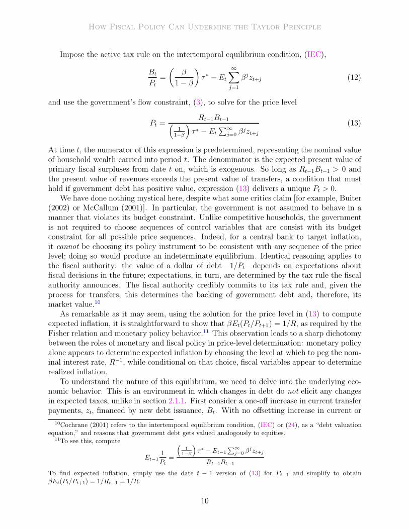
At time t, the numerator of this expression is predetermined, representing the nominal valueof household wealth carried into period t. The denominator is the expected present value ofprimary fiscal surpluses from date t on, which is exogenous. So long as Rt−1Bt−1 > 0 andthe present value of revenues exceeds the present value of transfers, a condition that musthold if government debt has positive value, expression (13) delivers a unique Pt > 0.

We have done nothing mystical here, despite what some critics claim [for example, Buiter(2002) or McCallum (2001)]. In particular, the government is not assumed to behave in amanner that violates its budget constraint. Unlike competitive households, the governmentis not required to choose sequences of control variables that are consist with its budgetconstraint for all possible price sequences. Indeed, for a central bank to target inflation,it cannot be choosing its policy instrument to be consistent with any sequence of the pricelevel; doing so would produce an indeterminate equilibrium. Identical reasoning applies tothe fiscal authority: the value of a dollar of debt—1/Pt—depends on expectations aboutfiscal decisions in the future; expectations, in turn, are determined by the tax rule the fiscalauthority announces. The fiscal authority credibly commits to its tax rule and, given theprocess for transfers, this determines the backing of government debt and, therefore, itsmarket value.10

As remarkable as it may seem, using the solution for the price level in (13) to computeexpected inflation, it is straightforward to show that βEt(Pt/Pt+1) = 1/R, as required by theFisher relation and monetary policy behavior.11 This observation leads to a sharp dichotomybetween the roles of monetary and fiscal policy in price-level determination: monetary policyalone appears to determine expected inflation by choosing the level at which to peg the nom-inal interest rate, R−1, while conditional on that choice, fiscal variables appear to determinerealized inflation.

To understand the nature of this equilibrium, we need to delve into the underlying eco-nomic behavior. This is an environment in which changes in debt do not elicit any changesin expected taxes, unlike in section 2.1.1. First consider a one-off increase in current transferpayments, zt, financed by new debt issuance, Bt. With no offsetting increase in current or

10Cochrane (2001) refers to the intertemporal equilibrium condition, (IEC) or (24), as a “debt valuationequation,” and reasons that government debt gets valued analogously to equities.

11To see this, compute

Et−1

1

Pt

=

(

1

1−β

)

τ∗ − Et−1

∑∞j=0

βjzt+j

Rt−1Bt−1

To find expected inflation, simply use the date t − 1 version of (13) for Pt−1 and simplify to obtainβEt(Pt/Pt+1) = 1/Rt−1 = 1/R.

10


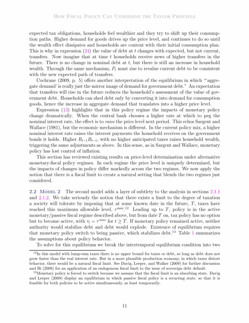
expected tax obligations, households feel wealthier and they try to shift up their consump-tion paths. Higher demand for goods drives up the price level, and continues to do so untilthe wealth effect dissipates and households are content with their initial consumption plan.This is why in expression (24) the value of debt at t changes with expected, but not current,transfers. Now imagine that at time t households receive news of higher transfers in thefuture. There is no change in nominal debt at t, but there is still an increase in householdwealth. Through the same mechanism, Pt must rise to revalue current debt to be consistentwith the new expected path of transfers.

Cochrane (2009, p. 5) offers another interpretation of the equilibrium in which “‘aggre-gate demand’ is really just the mirror image of demand for government debt.” An expectationthat transfers will rise in the future reduces the household’s assessment of the value of gov-ernment debt. Households can shed debt only by converting it into demand for consumptiongoods, hence the increase in aggregate demand that translates into a higher price level.

Expression (13) highlights that in this policy regime the impacts of monetary policychange dramatically. When the central bank chooses a higher rate at which to peg thenominal interest rate, the effect is to raise the price level next period. This echos Sargent andWallace (1981), but the economic mechanism is different. In the current policy mix, a highernominal interest rate raises the interest payments the household receives on the governmentbonds it holds. Higher Rt−1Bt−1, with no higher anticipated taxes raises household wealth,triggering the same adjustments as above. In this sense, as in Sargent and Wallace, monetarypolicy has lost control of inflation.

This section has reviewed existing results on price-level determination under alternativemonetary-fiscal policy regimes. In each regime the price level is uniquely determined, butthe impacts of changes in policy differ markedly across the two regimes. We now apply thenotion that there is a fiscal limit to create a natural setting that blends the two regimes justconsidered.

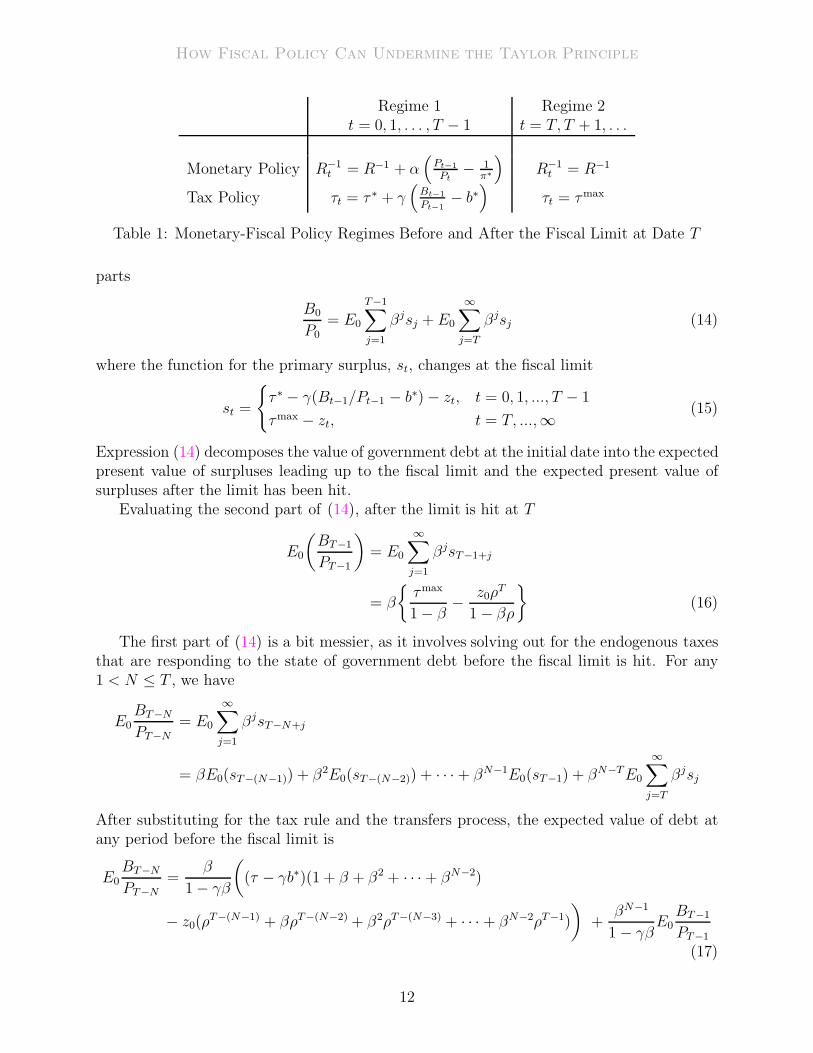
2.2 Model 2 The second model adds a layer of subtlety to the analysis in sections 2.1.1and 2.1.2. We take seriously the notion that there exists a limit to the degree of taxationa society will tolerate by imposing that at some known date in the future, T , taxes havereached this maximum allowable level, τmax.12 Leading up to T , policy is in the activemonetary/passive fiscal regime described above, but from date T on, tax policy has no optionbut to become active, with τt = τmax for t ≥ T . If monetary policy remained active, neitherauthority would stabilize debt and debt would explode. Existence of equilibrium requiresthat monetary policy switch to being passive, which stabilizes debt.13 Table 1 summarizesthe assumptions about policy behavior.

To solve for this equilibrium we break the intertemporal equilibrium condition into two

12In this model with lump-sum taxes there is no upper bound for taxes or debt, so long as debt does notgrow faster than the real interest rate. But in a more plausible production economy, in which taxes distortbehavior, there would be a natural fiscal limit. See Davig, Leeper, and Walker (2009) for further discussionand Bi (2009) for an application of an endogenous fiscal limit to the issue of sovereign debt default.

13Monetary policy is forced to switch because we assume that the fiscal limit is an absorbing state. Davigand Leeper (2009) display an equilibrium in which passive fiscal policy is a recurring state, so that it isfeasible for both policies to be active simultaneously, as least temporarily.

11


Regime 1 Regime 2t = 0, 1, . . . , T − 1 t = T, T + 1, . . .

Monetary Policy R−1t = R−1 + α

(

Pt−1

Pt

− 1π∗

)

R−1t = R−1

Tax Policy τt = τ ∗ + γ(

Bt−1

Pt−1

− b∗)

τt = τmax

Table 1: Monetary-Fiscal Policy Regimes Before and After the Fiscal Limit at Date T

parts

B0

P0= E0

T−1∑

j=1

βjsj + E0

∞∑

j=T

βjsj (14)

where the function for the primary surplus, st, changes at the fiscal limit

st =

{

τ ∗ − γ(Bt−1/Pt−1 − b∗) − zt, t = 0, 1, ..., T − 1

τmax − zt, t = T, ...,∞(15)

Expression (14) decomposes the value of government debt at the initial date into the expectedpresent value of surpluses leading up to the fiscal limit and the expected present value ofsurpluses after the limit has been hit.

Evaluating the second part of (14), after the limit is hit at T

E0

(

BT−1

PT−1

)

= E0

∞∑

j=1

βjsT−1+j

= β

{

τmax

1 − β−

z0ρT

1 − βρ

}

(16)

The first part of (14) is a bit messier, as it involves solving out for the endogenous taxesthat are responding to the state of government debt before the fiscal limit is hit. For any1 < N ≤ T , we have

E0BT−N

PT−N

= E0

∞∑

j=1

βjsT−N+j

= βE0(sT−(N−1)) + β2E0(sT−(N−2)) + · · · + βN−1E0(sT−1) + βN−TE0

∞∑

j=T

βjsj

After substituting for the tax rule and the transfers process, the expected value of debt atany period before the fiscal limit is

E0BT−N

PT−N

=β

1 − γβ

(

(τ − γb∗)(1 + β + β2 + · · · + βN−2)

− z0(ρT−(N−1) + βρT−(N−2) + β2ρT−(N−3) + · · · + βN−2ρT−1)

)

+βN−1

1 − γβE0

BT−1

PT−1

(17)

12


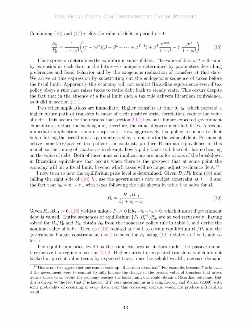
Combining (16) and (17) yields the value of debt in period t = 0

B0

P0=

1

1 − γβ

(

(τ − γb∗)(β + β2 + · · · + βT−1) + βT τmax

1 − β− z0

ρβ

1 − ρβ

)

(18)

This expression determines the equilibrium value of debt. The value of debt at t = 0—andby extension at each date in the future—is uniquely determined by parameters describingpreferences and fiscal behavior and by the exogenous realization of transfers at that date.We arrive at this expression by substituting out the endogenous sequence of taxes beforethe fiscal limit. Apparently this economy will not exhibit Ricardian equivalence even if taxpolicy obeys a rule that raises taxes to retire debt back to steady state. This occurs despitethe fact that in the absence of a fiscal limit such a tax rule delivers Ricardian equivalence,as it did in section 2.1.1.

Two other implications are immediate. Higher transfers at time 0, z0, which portend ahigher future path of transfers because of their positive serial correlation, reduce the valueof debt. This occurs for the reasons that section 2.1.2 lays out: higher expected governmentexpenditures reduce the backing and, therefore, the value of government liabilities. A secondimmediate implication is more surprising. How aggressively tax policy responds to debtbefore hitting the fiscal limit, as parameterized by γ, matters for the value of debt. Permanentactive monetary/passive tax policies, in contrast, produce Ricardian equivalence in thismodel, so the timing of taxation is irrelevant: how rapidly taxes stabilize debt has no bearingon the value of debt. Both of these unusual implications are manifestations of the breakdownin Ricardian equivalence that occurs when there is the prospect that at some point theeconomy will hit a fiscal limit, beyond which taxes will no longer adjust to finance debt.14

I now turn to how the equilibrium price level is determined. Given B0/P0 from (18) andcalling the right side of (18) b0, use the government’s flow budget constraint at t = 0 andthe fact that s0 = τ0 − z0, with taxes following the rule shown in table 1 to solve for P0:

P0 =R−1B−1

b0 + τ0 − z0

(19)

Given R−1B−1 > 0, (19) yields a unique P0 > 0 if b0+τ0−z0 > 0, which it must if governmentdebt is valued. Entire sequences of equilibrium {Pt, R

−1t }∞t=0 are solved recursively: having

solved for B0/P0 and P0, obtain R0 from the monetary policy rule in table 1, and derive thenomimal value of debt. Then use (18) redated at t = 1 to obtain equilibrium B1/P1 and thegovernment budget constraint at t = 1 to solve for P1 using (19) redated at t = 1, and soforth.

The equilibrium price level has the same features as it does under the passive mone-tary/active tax regime in section 2.1.2. Higher current or expected transfers, which are notbacked in present-value terms by expected taxes, raise household wealth, increase demand

14This is not to suggest that one cannot cook up “Ricardian scenarios.” For example, because T is known,if the government were to commit to fully finance the change in the present value of transfers that arisesfrom a shock to z0 before the economy reaches the fiscal limit, one could obtain a Ricardian outcome. Butthis is driven by the fact that T is known. If T were uncertain, as in Davig, Leeper, and Walker (2009), withsome probability of occurring at every date, even this cooked-up scenario would not produce a Ricardianresult.

13


for goods, and drive up the price level (reducing the value of debt). A higher pegged nom-inal interest rate raises nominal interest payments, raising wealth and the price level nextperiod. Similarities between this equilibrium and that in section 2.1.2 stem from the factthat price-level determination is driven by beliefs about policy in the long run. From T on,this economy is identical to the fixed-regime passive monetary/active fiscal policies economyand it is beliefs about long-run policies that determine the price level. Of course, before thefiscal limit the two economies are quite different and the behavior of the price level will alsobe different.

In this environment where the equilibrium price level is determined entirely by fiscalconsiderations through its interest rate policy, monetary policy determines the expectedinflation rate. Combining (4) with (5) we obtain an expression in expected inflation

Et

(

Pt

Pt+1−

1

π∗

)

=α

β

(

Pt−1

Pt

−1

π∗

)

(20)

where monetary policy behaves as table 1 specifies.As argued above, the equilibrium price level sequence, {Pt}

∞

t=0 is determined by versionsof (18) and (19) for each date t, so (20) describes the evolution of expected inflation. Givenequilibrium P0 from (19) and an arbitrary P−1—arbitrary because the economy starts att = 0 and cannot possibly determine P−1, regardless of policy behavior—(20) shows thatE0(P0/P1) grows relative to the initial inflation rate. In fact, throughout the active monetarypolicy/passive fiscal policy phase, for t = 0, 1, . . . , T −1, expected inflation grows at the rateαβ−1 > 1. In periods t ≥ T monetary policy pegs the nominal interest rate at R, andexpected inflation is constant: Et(Pt/Pt+1) = (Rβ)−1 = 1/π∗.

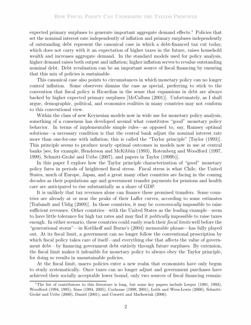
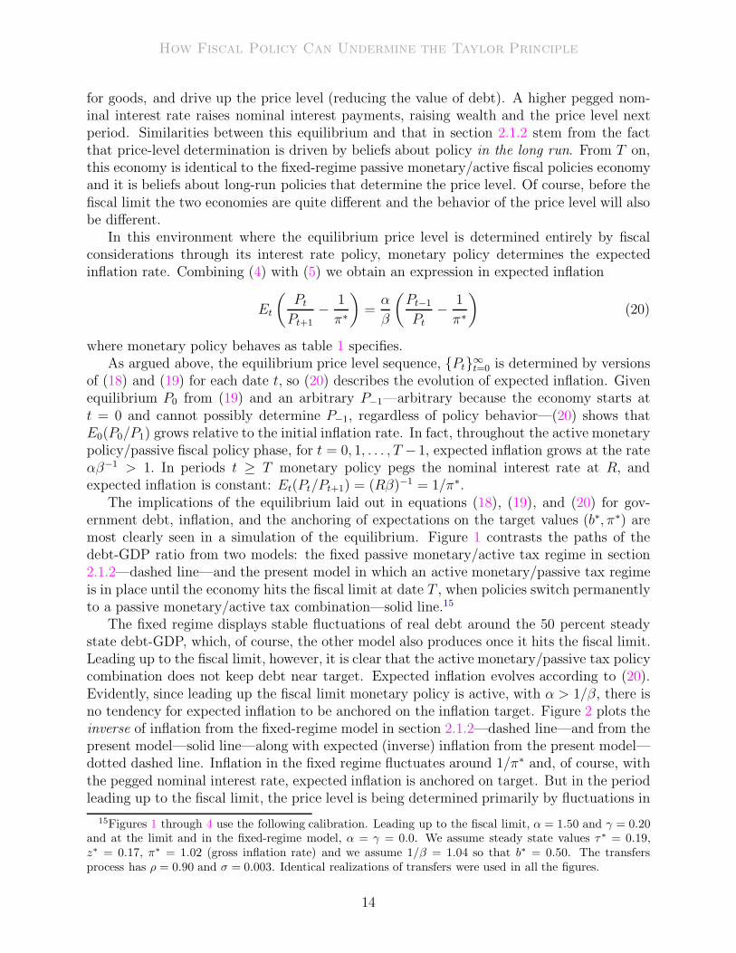
The implications of the equilibrium laid out in equations (18), (19), and (20) for gov-ernment debt, inflation, and the anchoring of expectations on the target values (b∗, π∗) aremost clearly seen in a simulation of the equilibrium. Figure 1 contrasts the paths of thedebt-GDP ratio from two models: the fixed passive monetary/active tax regime in section2.1.2—dashed line—and the present model in which an active monetary/passive tax regimeis in place until the economy hits the fiscal limit at date T , when policies switch permanentlyto a passive monetary/active tax combination—solid line.15

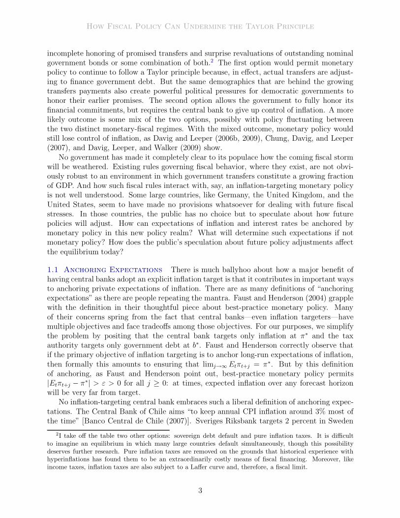
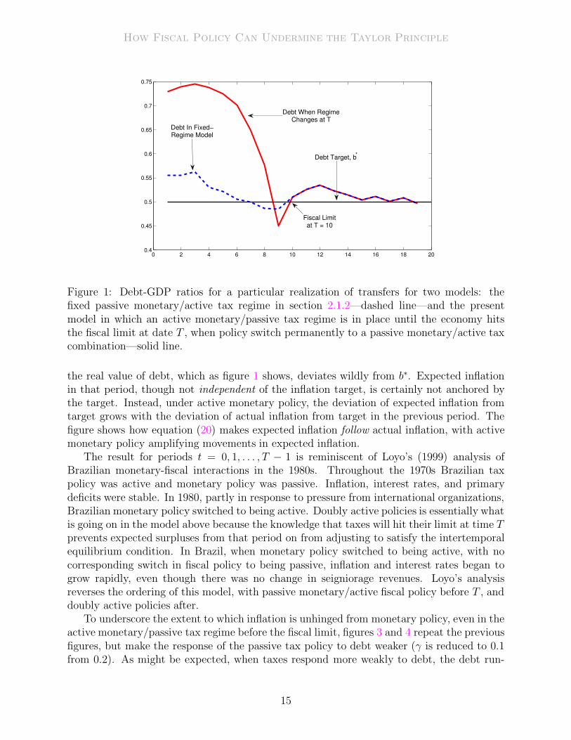
The fixed regime displays stable fluctuations of real debt around the 50 percent steadystate debt-GDP, which, of course, the other model also produces once it hits the fiscal limit.Leading up to the fiscal limit, however, it is clear that the active monetary/passive tax policycombination does not keep debt near target. Expected inflation evolves according to (20).Evidently, since leading up the fiscal limit monetary policy is active, with α > 1/β, there isno tendency for expected inflation to be anchored on the inflation target. Figure 2 plots theinverse of inflation from the fixed-regime model in section 2.1.2—dashed line—and from thepresent model—solid line—along with expected (inverse) inflation from the present model—dotted dashed line. Inflation in the fixed regime fluctuates around 1/π∗ and, of course, withthe pegged nominal interest rate, expected inflation is anchored on target. But in the periodleading up to the fiscal limit, the price level is being determined primarily by fluctuations in

15Figures 1 through 4 use the following calibration. Leading up to the fiscal limit, α = 1.50 and γ = 0.20and at the limit and in the fixed-regime model, α = γ = 0.0. We assume steady state values τ∗ = 0.19,z∗ = 0.17, π∗ = 1.02 (gross inflation rate) and we assume 1/β = 1.04 so that b∗ = 0.50. The transfersprocess has ρ = 0.90 and σ = 0.003. Identical realizations of transfers were used in all the figures.

14


0 2 4 6 8 10 12 14 16 18 200.4

0.45

0.5

0.55

0.6

0.65

0.7

0.75

Debt Target, b*

Fiscal Limitat T = 10

Debt When RegimeChanges at T

Debt In Fixed−Regime Model

Figure 1: Debt-GDP ratios for a particular realization of transfers for two models: thefixed passive monetary/active tax regime in section 2.1.2—dashed line—and the presentmodel in which an active monetary/passive tax regime is in place until the economy hitsthe fiscal limit at date T , when policy switch permanently to a passive monetary/active taxcombination—solid line.

the real value of debt, which as figure 1 shows, deviates wildly from b∗. Expected inflationin that period, though not independent of the inflation target, is certainly not anchored bythe target. Instead, under active monetary policy, the deviation of expected inflation fromtarget grows with the deviation of actual inflation from target in the previous period. Thefigure shows how equation (20) makes expected inflation follow actual inflation, with activemonetary policy amplifying movements in expected inflation.

The result for periods t = 0, 1, . . . , T − 1 is reminiscent of Loyo’s (1999) analysis ofBrazilian monetary-fiscal interactions in the 1980s. Throughout the 1970s Brazilian taxpolicy was active and monetary policy was passive. Inflation, interest rates, and primarydeficits were stable. In 1980, partly in response to pressure from international organizations,Brazilian monetary policy switched to being active. Doubly active policies is essentially whatis going on in the model above because the knowledge that taxes will hit their limit at time Tprevents expected surpluses from that period on from adjusting to satisfy the intertemporalequilibrium condition. In Brazil, when monetary policy switched to being active, with nocorresponding switch in fiscal policy to being passive, inflation and interest rates began togrow rapidly, even though there was no change in seigniorage revenues. Loyo’s analysisreverses the ordering of this model, with passive monetary/active fiscal policy before T , anddoubly active policies after.

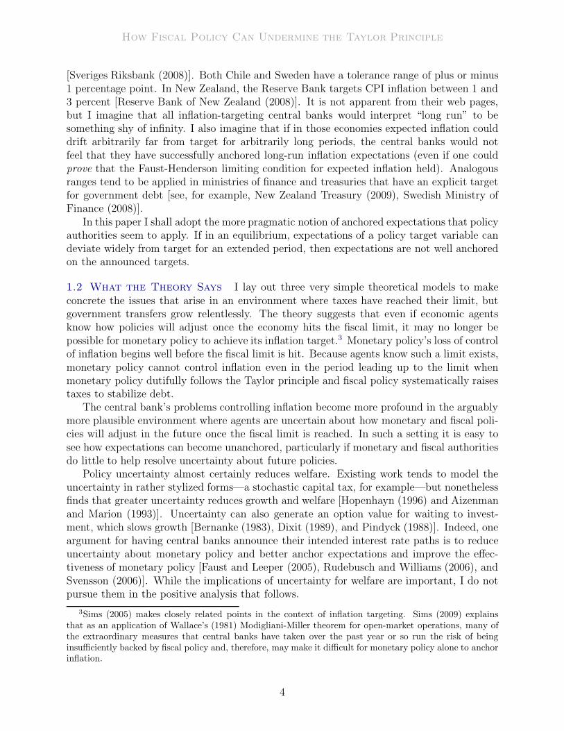
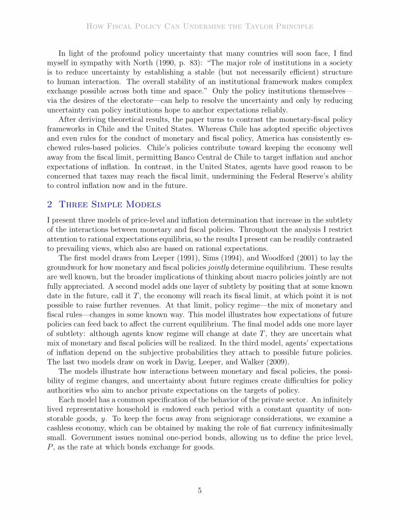
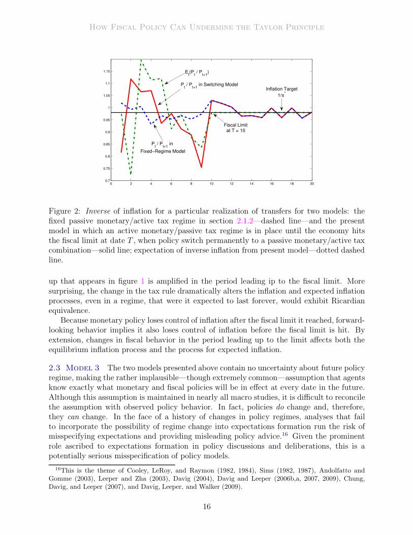
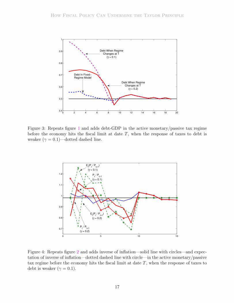
To underscore the extent to which inflation is unhinged from monetary policy, even in theactive monetary/passive tax regime before the fiscal limit, figures 3 and 4 repeat the previousfigures, but make the response of the passive tax policy to debt weaker (γ is reduced to 0.1from 0.2). As might be expected, when taxes respond more weakly to debt, the debt run-

15


0 2 4 6 8 10 12 14 16 18 200.7

0.75

0.8

0.85

0.9

0.95

1

1.05

1.1

1.15

Pt / P

t+1 in Switching Model

Pt / P

t+1 in

Fixed−Regime Model

Inflation Target

1/π*

Et(P

t / P

t+1)

Fiscal Limitat T = 10

Figure 2: Inverse of inflation for a particular realization of transfers for two models: thefixed passive monetary/active tax regime in section 2.1.2—dashed line—and the presentmodel in which an active monetary/passive tax regime is in place until the economy hitsthe fiscal limit at date T , when policy switch permanently to a passive monetary/active taxcombination—solid line; expectation of inverse inflation from present model—dotted dashedline.

up that appears in figure 1 is amplified in the period leading ip to the fiscal limit. Moresurprising, the change in the tax rule dramatically alters the inflation and expected inflationprocesses, even in a regime, that were it expected to last forever, would exhibit Ricardianequivalence.

Because monetary policy loses control of inflation after the fiscal limit it reached, forward-looking behavior implies it also loses control of inflation before the fiscal limit is hit. Byextension, changes in fiscal behavior in the period leading up to the limit affects both theequilibrium inflation process and the process for expected inflation.

2.3 Model 3 The two models presented above contain no uncertainty about future policyregime, making the rather implausible—though extremely common—assumption that agentsknow exactly what monetary and fiscal policies will be in effect at every date in the future.Although this assumption is maintained in nearly all macro studies, it is difficult to reconcilethe assumption with observed policy behavior. In fact, policies do change and, therefore,they can change. In the face of a history of changes in policy regimes, analyses that failto incorporate the possibility of regime change into expectations formation run the risk ofmisspecifying expectations and providing misleading policy advice.16 Given the prominentrole ascribed to expectations formation in policy discussions and deliberations, this is apotentially serious misspecification of policy models.

16This is the theme of Cooley, LeRoy, and Raymon (1982, 1984), Sims (1982, 1987), Andolfatto andGomme (2003), Leeper and Zha (2003), Davig (2004), Davig and Leeper (2006b,a, 2007, 2009), Chung,Davig, and Leeper (2007), and Davig, Leeper, and Walker (2009).

16


0 2 4 6 8 10 12 14 16 18 200.4

0.5

0.6

0.7

0.8

0.9

1


(γ = 0.1)


(γ = 0.2)

Debt In Fixed−Regime Model

Figure 3: Repeats figure 1 and adds debt-GDP in the active monetary/passive tax regimebefore the economy hits the fiscal limit at date T , when the response of taxes to debt isweaker (γ = 0.1)—dotted dashed line.

0 5 10 15

0.7

0.8

0.9

1

1.1

1.2 Pt / P

t+1

(γ = 0.1)

Pt / P

t+1

(γ = 0.2)

Et(P

t / P

t+1)

(γ = 0.2)

Et(P

t / P

t+1)

(γ = 0.1)

Figure 4: Repeats figure 2 and adds inverse of inflation—solid line with circles—and expec-tation of inverse of inflation—dotted dashed line with circle—in the active monetary/passivetax regime before the economy hits the fiscal limit at date T , when the response of taxes todebt is weaker (γ = 0.1).

17


I introduce uncertainty about policy in a stark fashion that allows me to extract someimplications of policy uncertainty while retaining analytical tractability. The economy con-tinues to hit the fiscal limit at a known date T , at which point taxes become active, settingτt = τmax for all t ≥ T . Uncertainty arises because at the limit agents place probability q ona regime that combines passive monetary policy with active transfers policy and probability1 − q on a regime with active monetary policy and passive transfers policy. In polite com-pany, passive transfers policy is referred to as “entitlements reform.”17 To avoid the tangleof euphemisms, I refer to this as “reneging on promised transfers.” Instead of receivingpromised transfers of zt at time t, agents receive λtzt, with λt ∈ [0, 1], so λt is the fraction ofpromised transfers that the government honors. Budget constraints for the household andthe government, equations (2) and (3), are modified to replace zt with λtzt.

Aging populations in many countries represent a looming fiscal crisis that offers a practicalmotivation for considering the possibility that governments may not honor their promises.Some countries—Australia, Chile, New Zealand, Norway, Sweden—are preparing for thedemographic shifts through the creation of superannuation funds or the adoption of fiscalrules that aim to have surpluses that can be saved to meet future government obligations.Other countries—Germany, the United Kingdom, the United States—are entering the periodof enhanced fiscal stress unprepared. In both sets of countries there is uncertainty aboutexactly how the government will finance its obligations, but in the unprepared countries,government reneging on promised transfers is a real possibility. This possibility potentiallyhas important impacts on expectations formation and economic decisions today.

For simplicity we reduce the previous models to just three periods. In the initial twoperiod (t = 0, 1), the fiscal limit has not been reached, promised transfers follow the process in(7), monetary policy is active and tax policy is passive. The economy begins with R−1B−1 >0 given and some arbitrary P−1. This is equivalent to the time period t = 0, . . . , T − 1 insection 2.2. At the beginning of period two (t = 2), the fiscal limit is reached but agentsremain uncertain about which mix of policies will be adopted. This uncertainty is resolvedat the end of period 2. In period 3, there is no uncertainty about policy and therefore, period3 is completely analogous to section 2.2 for t = T, T + 1, . . ..

Combining the Fisher relation, (4), with the active monetary policy rule, (5), for periods0 and 1 yields

E0

(

P1

P2−

1

π∗

)

=α2

β2

(

P−1

P0−

1

π∗

)

(21)

and combining the government budget constraint, (3), with the passive tax rule, (6), yields

E0

(

B1

P1− b∗

)

= E0(z1 − z∗) + (β−1 − γ)

(

B0

P0− b∗

)

(22)

Agents know that in the next period (t = 2) the fiscal limit will be reached and policywill switch to either a passive monetary/active transfers regime with probability q, or an

17To quote the New York Times, “Just about everybody agrees that solving the deficit depends on reducingthe benefits that current law has promised to retirees, via Medicare and Social Security. That’s not howpeople usually put it, of course. They tend to use the more soothing phrase ‘entitlement reform.’ Butentitlement reform is just another way of saying that we can’t pay more in benefits than we collect in taxes”[Leonhardt (2009)].

18


active monetary/passive transfers regime with probability (1−q). Assume that the renegingrate is fixed and known at t = 0, so λ2 = λ3 = λ ∈ [0, 1]. Then the conditional probabilitydistribution of these policies is given by

{

q R−12 = R−1, z2 = ρz1 + ε2

(1 − q) R−12 = R−1 + α

(

P1

P2

− 1π∗

)

, λz2 = λρz1 + λε2

The analogs of (21) and (22) for period 2 are

E2

(

P2

P3−

1

π∗

)

= (1 − q)α

β

(

P1

P2−

1

π∗

)

(23)

E1

(

B2

P2− b∗

)

= [q + (1 − q)λ]E1z2 − z∗ + β−1

(

B1

P1− b∗

)

(24)

In (24), to make the relationships transparent, I have imposed that τmax = τ ∗, the steadystate level of taxes.

In period 3, τ3 is set to completely retire debt (B3 = 0) no matter which policy regime isrealized in period 2. This corresponds to τ3 = δz3 + (R2B2)/P3, where δ = 1 if the economyis in the passive monetary/active transfers regime and δ = λ if the active monetary/passivetransfer regime is realized. This assumption implies that agents know one period in advancewhich tax policy will be in place in the final period.

Combining (21) and (23), we obtain a relationship between expected inflation betweenperiods 2 and 3 and actual inflation in the initial period

E0

(

P2

P3

−1

π∗

)

= (1 − q)α3

β3

(

P−1

P0

−1

π∗

)

(25)

Given the discount rate β, this solution for expected inflation shows that whether expectedinflation converges to target or drifts from target depends on the probability of switching topassive monetary/active transfers policies relative to how hawkishly monetary policy targetsinflation when it is active. For the deviation of expected inflation from target to be smallerthan the deviation of actual inflation from target in period t = 0, we need q > 1 − (β/α)3.The longer the period leading up to the fiscal limit, the larger must q be to ensure that (25)is stable. It may seem paradoxical, but the more hawkish is policy—larger α—the greatermust be the probability that monetary policy will be passive (“dovish?”) in the future inorder for the evolution of expected inflation to be stable. Resolution of this paradox comesfrom recognizing that when q = 1, so monetary policy is known to be passive at the fiscallimit, expected inflation is anchored on π∗, whereas when q = 0, so transfers policy is knownto be passive at the limit, then (25) yields equilibrium inflation, just as in section 2.1.1.

Since we assume that taxes in period 3 are known, and they are a function of exogenousobjects, we can treat τ3 as fixed. Combining (22) and (24) and imposing that B3 = 0, as isthe debt target in the last period,

B0

P0− b∗ =

(

1

β−1 − γ

)

E0

{

β2{(τ3 − τ ∗) − (ϑz3 − z∗)]

− β(ϑz2 − z∗) − (z1 − z∗) (26)

where ϑ = q + (1 − q)λ determines expected post-reneging transfers.

19


Equation (26) uniquely determines the value of debt in period 0 as a function of theexpected present value of surpluses. We can combine (26) with the government’s flow con-straint at t = 0 to obtain a unique expression for P0 as a function of R−1B−1, τ0, z0, and theparameters in the expression for equilibrium B0/P0.

The solution in (26) leads to the following inferences. As q—the probability of switchingto the passive monetary/active transfers regime—rises, the value of debt at 0 falls, andP0 rises. In addition, as λ—the fraction of transfers on which the government reneges inperiods 2 and 3—falls, the value of debt at 0 falls, and the price level rises. Both of theconsequences for P0 operate through standard fiscal theory wealth effects. Higher q meansthere is less likelihood that the government will renege, so expected transfers and, therefore,household wealth rise. Households attempt to convert the higher wealth into consumptiongoods, driving up the price level until real wealth falls sufficiently that they are contentto consume their original consumption place. Lower λ also raises the expected value oftransfers, increasing wealth and the price level.

Expectational effects associated with switching policies can be seen explicitly in (25)and (26). Equation (26) shows that the value of debt is still determined by the discountedexpected value of net surpluses. In contrast to the previous models without uncertaintyabout future policies, now the actual surplus is conditional on the realized policy regime.Conditional on time t = 0 information, the expected transfers process in periods 2 and 3 isunknown. If q ∈ (0, 1) and at the end of period two passive monetary policy is realized, agentswill be “surprised” by amount z2(1 − q)(1 − λ) in period 2 and by amount z3(1 − q)(1 − λ)in period 3. With transfers surprisingly high—because the passive transfers regime withreneging was not realized—households feel wealthier and try to convert that wealth intoconsumption. This drives up the price level in periods 2 and 3, revaluing debt downward.This surprise acts as an innovation to the agent’s information set due to policy uncertainty.Naturally, as agents put high probability on this regime occurring (q ≈ 1) or assumes theamount of reneging is small (λ2, λ3 ≈ 1), the surprise is also small, and vice versa.

Comparing (25) with (20), expected inflation in period 1 now depends on q, which sum-marizes beliefs about future policies. This is true even though the monetary policy regimeis active in period 1. The previous model demonstrated that monetary policy alone cannotdetermine the price level. With policy uncertainty, monetary policy alone cannot determineexpected inflation. If agents put high probability on the passive monetary/active transfersregime (q ≈ 1), then expected inflation at the beginning of period 2 will be primarily pinneddown by the nominal peg. This result is irrespective of the actual policy regime announcedat the end of period 2. It is in this sense that expectational effects about policy uncertaintycan dramatically alter equilibrium outcomes.

In this simple setup, these expectational effects are limited in magnitude because agentsknow precisely when the fiscal limit is reached. The additional level of uncertainty not exam-ined in these simple models, but present in Davig, Leeper, and Walker (2009), is randomnessin when tax policy will hit the the fiscal limit. In that environment, the conditional prob-ability of switching policies outlined above would contain an additional term specifying theconditional probability of hitting the fiscal limit in that period. This implies that, becausethere is positive probability of hitting the fiscal limit in every period up to T , these expec-tational effects will be present from t = 0, . . . , T and will gradually become more importantas the probability of hitting the fiscal limit increases. In effect, the endogenous probability

20


of hitting the fiscal limit makes the probability q time varying.

2.4 Summary The models presented above severely understate the degree of uncertaintyabout future policies that private agents face in actual economies. To derive a rationalexpectations equilibrium, I have taken stands on the stochastic structure of the economythat are difficult to reconcile with observations about any actual policy environment.18

Remarkably, the models show that even in a setting that drastically understates the actual

degree of uncertainty, private expectations of monetary and fiscal objectives are not wellanchored on the targets of policy. These models also make clear that in an economy thatfaces heightened fiscal stress, the monetary policy behavior that most economists regardas “good” cannot control either actual or expected inflation. “Good” monetary policy canactually exaggerate the swings in expected inflation.

3 Policy Institutions and Future Policies

This section examines monetary and fiscal policy arrangements in Chile and the UnitedStates to draw some inferences about how the theoretical points derived above might playout in those economies. Chile and America offer interesting contrasts. Whereas Chile hasadopted specific objectives and even rules for the conduct of monetary and fiscal policy,America has eschewed rules-based policies. Banco Central de Chile is guided by an explicitinflation target; the Federal Reserve operates under a multiple mandate. Chile has adopteda series of fiscal rules, designed in part to provide for its aging population; the United Stateshas done nothing except implement short-run fiscal policies that are projected to double theoutstanding debt over the next decade. For the theme of this paper—how macro policies door do not anchor expectations—the contrast is particularly relevant.

3.1 The United States Even in normal times, the multiple objectives that guide FederalReserve decisions and the absence of any mandates to guide federal tax and spending policiesconspire to make it very difficult for private agents to form expectations of monetary andfiscal policies.19

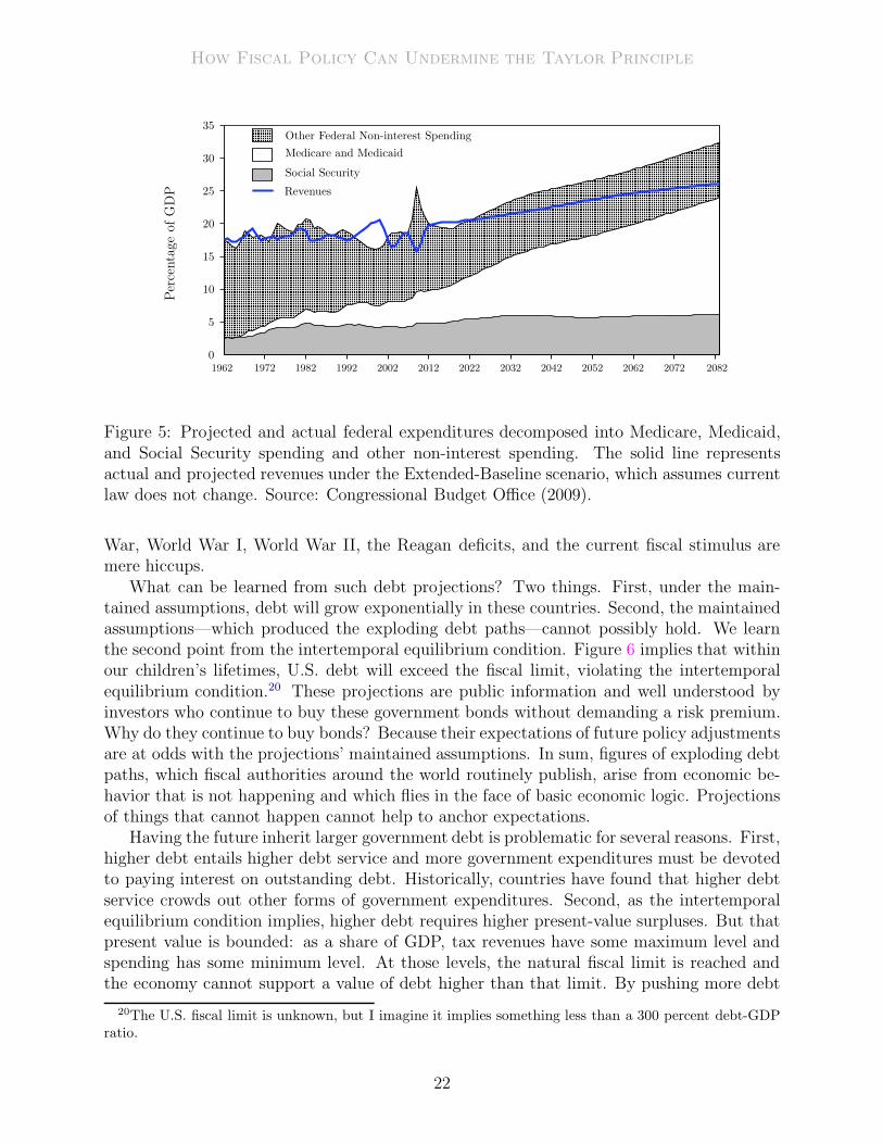
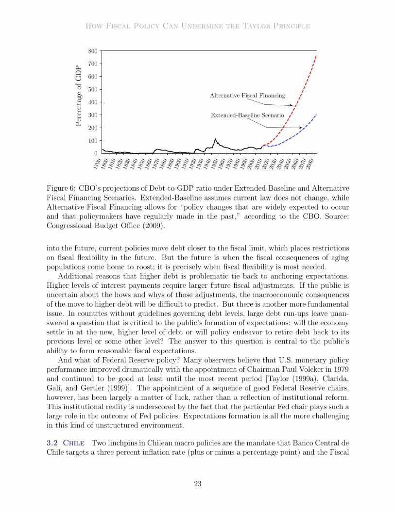
In the United States, the Congressional Budget Office (CBO) regularly publishes pro-jections of the country’s long-run fiscal situation. In the wake of the financial crisis andrecession of 2007-2009, monetary and fiscal policies have not been normal and, as long-termprojections by the CBO make plain, in the absence of dramatic policy changes, policies areunlikely to return to normalcy for generations to come. Figure 5 reports actual and CBOprojections of federal transfers due to Social Security, Medicaid, and Medicare as a percent-age of GDP [Congressional Budget Office (2009)]. Demographic shifts and rising relativecosts of health care combine to grow these transfers from under 10 percent of GDP today toabout 25 percent in 70 years. One much-discussed consequence of this growth is shown infigure 6, which plots actual and CBO projections of federal government debt as a share ofGDP from 1790 to 2083. Relative to the future, the debt run-ups associated with the Civil

18Sargent (2006) acknowledges this and goes so far as to say that American monetary and fiscal policies aremarked by “ambiguity or Knightian uncertainty,” which preclude the specificity about stochastic structureassumed in the models of section 2.

19This section draws heavily on Leeper (2009) and Davig, Leeper, and Walker (2009).

21


Other Federal Non-interest Spending

Medicare and Medicaid

Social Security

1962 1972 1982 1992 2002 2012 2022 2032 2042 2052 2062 2072 2082

0

5

10

15

20

25

30

35

Per

centa

ge

ofG

DP

��

��

�

�

�

�

�

�

�

�

�

�

�

� �

�

� �

�

��

��

��

�

��

�

�

�

�

�

�

�

�

�

�

�

�

�

�

��

�

�

�

�

�

��

� � � � ��

��

��

��

� ��

��

��

��

� ��

��

��

��

��

��

��

� ��

��

��

��

� � ��

� ��

� ��

��

� � ��

��

�

� � Revenues

Figure 5: Projected and actual federal expenditures decomposed into Medicare, Medicaid,and Social Security spending and other non-interest spending. The solid line representsactual and projected revenues under the Extended-Baseline scenario, which assumes currentlaw does not change. Source: Congressional Budget Office (2009).

War, World War I, World War II, the Reagan deficits, and the current fiscal stimulus aremere hiccups.

What can be learned from such debt projections? Two things. First, under the main-tained assumptions, debt will grow exponentially in these countries. Second, the maintainedassumptions—which produced the exploding debt paths—cannot possibly hold. We learnthe second point from the intertemporal equilibrium condition. Figure 6 implies that withinour children’s lifetimes, U.S. debt will exceed the fiscal limit, violating the intertemporalequilibrium condition.20 These projections are public information and well understood byinvestors who continue to buy these government bonds without demanding a risk premium.Why do they continue to buy bonds? Because their expectations of future policy adjustmentsare at odds with the projections’ maintained assumptions. In sum, figures of exploding debtpaths, which fiscal authorities around the world routinely publish, arise from economic be-havior that is not happening and which flies in the face of basic economic logic. Projectionsof things that cannot happen cannot help to anchor expectations.

Having the future inherit larger government debt is problematic for several reasons. First,higher debt entails higher debt service and more government expenditures must be devotedto paying interest on outstanding debt. Historically, countries have found that higher debtservice crowds out other forms of government expenditures. Second, as the intertemporalequilibrium condition implies, higher debt requires higher present-value surpluses. But thatpresent value is bounded: as a share of GDP, tax revenues have some maximum level andspending has some minimum level. At those levels, the natural fiscal limit is reached andthe economy cannot support a value of debt higher than that limit. By pushing more debt

20The U.S. fiscal limit is unknown, but I imagine it implies something less than a 300 percent debt-GDPratio.

22


1790

1800

1810

1820

1830

1840

1850

1860

1870

1880

1890

1900

1910

1920

1930

1940

1950

1960

1970

1980

1990

2000

2010

2020

2030

2040

2050

2060

2070

2080

0

100

200

300

400

500

600

700

800

Per

centa

ge

ofG

DP

Alternative Fiscal Financing

Extended-Baseline Scenario

� � �

��

��

� � � � � � � � � � � ��

� � � � � � � � � � � � � � � � � ��

� � � � � � � � �

�

�

��

� � � � � ��

��

��

� � � � � � � � � � � � � � � � � � � � � � � � � � � � � � � � � � �

�

��

�

� �

� ��

� � ��

�

�

�

� � ��

� � � �

�

�

�

�

�

�

� �

�

� ��

�

�

��

� � � � ��

�

� ��

� � � ��

� � � � � � �

�

� ��

� � � � �

��

��

�

� � ��

�

�

�

� � ��

��

��

�

�

�

�

�

�

�

�

�

�

�

�

�

�

�

�

�

�

�

�

�

�

�

�

�

�

�

�

�

�

�

�

�

�

�

�

�

�

�

�

�

�

�

�

�

�

�

�

�

�

�

�

�

�

�

�

�

�

�

�

�

�

�

�

�

� � � � � � � � � � � � � � � � ��

��

��

��

�

��

��

�

��

�

�

��

�

�

�

�

�

�

�

�

�

�

�

�

�

�

�

�

�

�

�

�

�

�

�

�

�

�

�

�

�

�

�

�

�

�

�

�

�

�

�

�

Figure 6: CBO’s projections of Debt-to-GDP ratio under Extended-Baseline and AlternativeFiscal Financing Scenarios. Extended-Baseline assumes current law does not change, whileAlternative Fiscal Financing allows for “policy changes that are widely expected to occurand that policymakers have regularly made in the past,” according to the CBO. Source:Congressional Budget Office (2009).

into the future, current policies move debt closer to the fiscal limit, which places restrictionson fiscal flexibility in the future. But the future is when the fiscal consequences of agingpopulations come home to roost; it is precisely when fiscal flexibility is most needed.

Additional reasons that higher debt is problematic tie back to anchoring expectations.Higher levels of interest payments require larger future fiscal adjustments. If the public isuncertain about the hows and whys of those adjustments, the macroeconomic consequencesof the move to higher debt will be difficult to predict. But there is another more fundamentalissue. In countries without guidelines governing debt levels, large debt run-ups leave unan-swered a question that is critical to the public’s formation of expectations: will the economysettle in at the new, higher level of debt or will policy endeavor to retire debt back to itsprevious level or some other level? The answer to this question is central to the public’sability to form reasonable fiscal expectations.

And what of Federal Reserve policy? Many observers believe that U.S. monetary policyperformance improved dramatically with the appointment of Chairman Paul Volcker in 1979and continued to be good at least until the most recent period [Taylor (1999a), Clarida,Galı, and Gertler (1999)]. The appointment of a sequence of good Federal Reserve chairs,however, has been largely a matter of luck, rather than a reflection of institutional reform.This institutional reality is underscored by the fact that the particular Fed chair plays such alarge role in the outcome of Fed policies. Expectations formation is all the more challengingin this kind of unstructured environment.

3.2 Chile Two linchpins in Chilean macro policies are the mandate that Banco Central deChile targets a three percent inflation rate (plus or minus a percentage point) and the Fiscal

23


Responsibility Law.21 The Basic Constitutional Act of the Central Bank of Chile, passed in1989, granted the central bank full independence and prescribed price stability and smoothfunctioning of the payments systems as its objectives. A formal inflation target was adoptedin 2007, with the aim of hitting three percent inflation “in a medium term horizon of twoyears.” As with many inflation targeting central banks, along with the explicit target cameenhanced transparency and an emphasis on communication with the public.

Although many countries adopted inflation targeting without also implementing a com-patible fiscal framework, Chile has been at the vanguard of countries that have reformedtheir monetary and fiscal policy institutions jointly. Chilean fiscal policy has been guided bya structural surplus rule since 2000 and the rule was given some legal teeth by the passage ofthe Fiscal Responsibility Law in August 2006. In the beginning, the ruled aimed for a struc-tural surplus of 1 percent of GDP. But the target itself is state dependent: it was changedto 0.5 percent in 2008 and since January 2009 it was changed again, explicitly temporarily,to aim to balance the budget.

Like many Latin American countries, Chilean fiscal policy was strongly procyclical, whichexacerbated cyclical fluctuations.22 The structural balance methodology, and the associatedsurplus rule, were designed to counter the procyclicality, among several other key goals. Toarrive at the structural surplus, the government estimates what revenues it would receive ifthe economy were growing at trend and the prices of copper and molybdenum were at theirlong-run levels.23 For the first six years the aim of the surplus was to accumulate assetsthat could be used to meet future government obligations, particularly guaranteed minimumpensions and old-age transfer payments.

Benefits from the adoption of the structural surplus rule have been remarkable. Somekey benefits include

1. Chilean fiscal policy has been freed to behave countercyclically.

2. Government debt and interest payments on debt fell through the 2000s, with grosscentral debt down to 5 percent of GDP in 2008.

3. Establishment of a Pension Reserve Fund whose assets are invested, just as privatepension funds are invested, and accumulated to meet future obligations.24

4. Sovereign debt interest-rate spreads for Chile are now well below those of other emerg-ing economies and did not rise after 9/11 or the Argentine crisis of 2002, when othercountries’ spread rose sharply; the decline in Chilean spreads began with the adoptionof the structural balance policy.

21This section draws on several sources, including Perry, Serven, and Suescun (2008), Singh, Belaisch,Collyns, De Masi, Krieger, Meredith, and Rennhack (2005), Rodrıguez C., Tokman R., and Vega C. (2007),Marshall (2003), Banco Central de Chile (2007), Velasco (2008), and International Monetary Fund (2009).

22Procyclicality and its consequences are documented in Gavin and Perotti (1997) and Kaminsky, Reinhart,and Vegh (2004).

23Batini, Levine, and Pearlman (2009) and Kumhof and Laxton (2009) assess the performance of such arule in dynamic stochastic general equilibrium models.

24Several countries have similar funds. Norway has created a large sovereign wealth fund from oil revenues;Australia and New Zealand have superannuation funds.

24


5. Declining sovereign debt risk spreads speak directly to the improved prospects forsustainability of Chile’s fiscal policies.

Items 4 and 5 cut on the paper’s theme of anchoring expectations and, therefore, deserveelaboration.25 Small open economies are susceptible to large external shocks that make theeconomies highly volatile. This tendency is still more pronounced in economies, like Chile,that are strongly affected by fluctuations in commodity prices. Bi (2009) shows theoreticallythat default risk premia emerge from the market’s expectations about a country’s ability andwillingness to service its debt. Ability arises endogenously from the country’s stochastic fiscallimit, which is tied to the peak of the country’s Laffer curve. The probability distribution ofthe fiscal limit depends on how persistent and volatile technology shocks are, the size of thegovernment, the degree of countercyclicality of fiscal policies, and the impatience of politicaldecisionmakers. Volatile economies tend to have highly dispersed distributions for the fiscallimit, which increase the probability of default at any given debt-GDP ratio; countries withlarge government transfer programs have fiscal limits with lower means; impatient politicalleaders reduce the mean of the limit.

A country’s willingness to service debt is driven by the flexibility of its fiscal policy.Flexible policy implies a willingness to raise taxes or lower government expenditures in theface of debt run-ups. A country that is operating well below its fiscal limit and is willing toadjust surpluses to stabilize debt, can successfully steer its way through economic downturnswithout incurring the wrath of financial markets in the form of risk premia.

Viewed in the context of fiscal limits, Chile’s structural balance rule and related inno-vations stemming from Fiscal Responsibility Law serve to move Chile’s government debtposition farther from the fiscal limit. Greater distance from the limit arises from both re-duced government debt today and from effectively shifting the distribution of the limit upto higher debt-GDP levels. Shifts in the distribution of the fiscal limit come from forcinga longer-term perspective on fiscal decisions and by creating reserves that can be tapped inthe future to finance benefits to the aging population. In this sense, the structural balancerule contributes in important ways to anchoring expectations on sustainable policies thatare well cushioned away from Chile’s fiscal limit.

As the theory in this paper implies, so long as the probability of hitting the fiscal limitin Chile is remote, there is every reason to believe that Banco Central de Chile’s efforts atinflation targeting will continue to be successful.

4 Concluding Remarks

Many countries are entering an extended period of relentless growth in transfer paymentspromised to their aging populations. Some, but not all, of these countries ultimately arerelying on a pay-as-you-go scheme for financing these expenditures. If there is a level oftaxation that, for economic or political reasons, those economies cannot exceed, then thepay-as-you-go scheme is unsustainable.

As Herb Stein famously said, “If something cannot go on forever, it will stop.” Steinalso pointed out that, although economists are good at pointing out when something cannot

25This discussion is based on the insightful study of fiscal limits and sovereign debt risk premia by Bi(2009).

25


persist indefinitely, they are less adept at predicting when it will stop. True enough in thepresent context. But we can say something constructive. Economic agents’ beliefs aboutwhen the economy will reach its fiscal limit and how policies will adjust after the limit willfeedback to affect the equilibrium we observe today, before the limit is reached. Predictingwhen an economy will hit its fiscal limit is less important for policymaking than is thesystematic analysis of the possible existence of such a limit and all that that implies aboutexpectations and macro policy effects.

For policymakers, the feedback from beliefs about the limit to the current equilibriumshould be disturbing. Because pre-limit economic decisions depend in part of beliefs aboutpost-limit policy behavior, accurate predictions of the impacts of policy changes today relyon understanding to what those beliefs are anchored. Coherent monetary-fiscal frameworkscan help to anchor those beliefs. Incoherent frameworks can actually make beliefs even moreuntethered.

Countries can guard against this eventuality by implementing monetary-fiscal frameworksthat keep their debt-GDP ratios well away from their fiscal limits.26 But fiscal limits arecountry specific and depend on myriad things that characterize a country’s political-economicenvironment. No one-size-fits-all policy framework will work across a highly diverse set ofcountries.

Chile has instituted a monetary-fiscal framework that, at least for now, appears to bemoving the country farther from its fiscal limit. With sufficient distance from that limit,there is reason to believe that Banco Central de Chile’s pursuit of inflation targeting cansuccessfully anchor actual and expected inflation. Progress has been far slower—or non-existent—in many larger countries. And even responsible countries may bear some of thecosts created by those large countries.

26Of course, there is a delicate balancing act here, since high tax rates and low government infrastructurespending, which could keep debt low, are also socially costly.

26


References

Aizenman, J., and N. Marion (1993): “Policy Uncertainty, Persistence and Growth,”Review of International Economics, 1(2), 145–163.

Andolfatto, D., and P. Gomme (2003): “Monetary Policy Regimes and Beliefs,” Inter-

national Economic Review, 44(1), 1–30.

Banco Central de Chile (2007): Central Bank of Chile: Monetary Policy in an Inflation

Targeting Framework. Banco Central de Chile, Santiago.

Batini, N., P. Levine, and J. Pearlman (2009): “Monetary and Fiscal Rules in anEmerging Small Open Economy,” IMF Working Paper WP/09/22.

Bernanke, B. S. (1983): “Irreversibility, Uncertainty, and Cyclical Investment,” Quarterly

Journal of Economics, 98(1), 85–106.

Bi, H. (2009): “Sovereign Risk Premia, Fiscal Limits and Fiscal Policy,” Manuscript, Indi-ana University.

Buiter, W. H. (2002): “The Fiscal Theory of the Price Level: A Critique,” Economic

Journal, 112(481), 459–480.

Cagan, P. (1956): “The Monetary Dynamics of Hyperinflation,” in Studies in the Quantity

Theory of Money, ed. by M. Friedman, pp. 25–117. University of Chicago Press, Chicago.

Chung, H., T. Davig, and E. M. Leeper (2007): “Monetary and Fiscal Policy Switch-ing,” Journal of Money, Credit and Banking, 39(4), 809–842.

Clarida, R., J. Galı, and M. Gertler (1999): “The Science of Monetary Policy: ANew Keynesian Perspective,” Journal of Economic Literature, 37(4), 1661–1707.

Cochrane, J. H. (1999): “A Frictionless View of U.S. Inflation,” in NBER Macroeconomics

Annual 1998, ed. by B. S. Bernanke, and J. J. Rotemberg, vol. 14, pp. 323–384. MIT Press,Cambridge, MA.

(2001): “Long Term Debt and Optimal Policy in the Fiscal Theory of the PriceLevel,” Econometrica, 69(1), 69–116.

(2007): “Inflation Determination with Taylor Rules: A Critical Review,”Manuscript, University of Chicago.

(2009): “Understanding Fiscal and Monetary Policy in 2008-2009,” Manuscript,University of Chicago.

Congressional Budget Office (2009): The Long-Term Budget Outlook. CBO, Wash-ington, D.C., June.

Cooley, T. F., S. F. LeRoy, and N. Raymon (1982): “Modeling Policy Interventions,”Manuscript, University of California Santa Barbara.

27


(1984): “Econometric Policy Evaluation: Note,” American Economic Review, 74(3),467–470.

Corsetti, G., and B. Mackowiak (2006): “Fiscal Imbalances and the Dynamics ofCurrency Crises,” European Economic Review, 50(5), 1317–1338.

Daniel, B. C. (2001): “The Fiscal Theory of the Price Level in an Open Economy,” Journal

of Monetary Economics, 48(October), 293–308.

Davig, T. (2004): “Regime-Switching Debt and Taxation,” Journal of Monetary Eco-

nomics, 51(4), 837–859.

Davig, T., and E. M. Leeper (2006a): “Endogenous Monetary Policy Regime Change,”in NBER International Seminar on Macroeconomics 2006, ed. by L. Reichlin, and K. D.West, pp. 345–377. MIT Press, Cambridge, MA.

(2006b): “Fluctuating Macro Policies and the Fiscal Theory,” in NBER Macroe-

conomics Annual 2006, ed. by D. Acemoglu, K. Rogoff, and M. Woodford, vol. 21, pp.247–298. MIT Press, Cambridge.

(2007): “Generalizing the Taylor Principle,” American Economic Review, 97(3),607–635.

(2009): “Monetary-Fiscal Policy Interactions and Fiscal Stimulus,” NBER WorkingPaper No. 15133.

Davig, T., E. M. Leeper, and T. B. Walker (2009): “‘Unfunded Laibilities’ andUncertain Fiscal Financing,” Manuscript, Indiana University.

Dixit, A. K. (1989): “Entry and Exit Decisions Under Uncertainty,” Journal of Political

Economy, 97(3), 620–638.

Faust, J., and D. W. Henderson (2004): “Is Inflation Targeting Best-Practice MonetaryPolicy?,” Federal Reserve Bank of St. Louis Economic Review, 86(4), 117–143.

Faust, J., and E. M. Leeper (2005): “Forecasts and Inflation Reports: An Evaluation,”Manuscript, Indiana University.

Galı, J. (2008): Monetary Policy, Inflation, and the Business Cycle. Princeton UniversityPress, Princeton.

Gavin, M., and R. Perotti (1997): “Fiscal Policy in Latin America,” in NBER Macroe-

conomics Annual 1997, ed. by B. S. Bernanke, and J. Rotemberg, vol. 12, pp. 11–61. MITPress, Canbridge, MA.

Henderson, D. W., and W. McKibbin (1993): “An Assessment of Some Basic MonetaryPolicy Regime Pairs: Analytical and Simulation Results from Simple Multiregion Macroe-conomic Models,” in Evaluating Policy Regimes: New Research in Empirical Macroeco-

nomics, ed. by R. C. Bryant, P. Hooper, and C. L. Mann. The Brookings Institution,Washington, D.C.

28


Hopenhayn, H. (1996): “Policy Variability and Economic Growth,” Review of Economic

Studies, 63(4), 611–625.

International Monetary Fund (2009): “Chile: Selected Issues,” IMF Country ReportNo. 09/272, September.

Kaminsky, G. L., C. M. Reinhart, and C. A. Vegh (2004): “When It Rains, It Pours:Procyclical Capital Flows and Macroeconomic Policies,” in NBER Macroeconomics Annual

2004, ed. by M. Gertler, and K. Rogoff, vol. 19, pp. 11–53. MIT Press, Cambridge, MA.

Kotlikoff, L. J., and S. Burns (2004): The Coming Generational Storm: What You

Need to Know About America’s Economic Future. MIT Press, Cambridge, MA.

Kumhof, M., and D. Laxton (2009): “Chile’s Structureal Fiscal Surplus Rule: A Model-Based Evaluation,” IMF Working Paper WP/09/88.

Leeper, E. M. (1991): “Equilibria Under ‘Active’ and ‘Passive’ Monetary and Fiscal Poli-cies,” Journal of Monetary Economics, 27(1), 129–147.

(1993): “The Policy Tango: Toward a Holistic View of Monetary and Fiscal Effects,”Federal Reserve Bank of Atlanta Economic Review, 78(4), 1–27.

(2009): “Anchoring Fiscal Expectations,” Reserve Bank of New Zealand Bulletin,72(3), 7–32.

Leeper, E. M., and T. Zha (2003): “Modest Policy Interventions,” Journal of Monetary

Economics, 50(8), 1673–1700.

Leith, C., and S. Wren-Lewis (2000): “Interactions between Monetary and Fiscal PolicyRules,” The Economic Journal, 110(462), 93–108.

Leonhardt, D. (2009): “A Drop in the Wrong Bucket,” New York Times, October 29.

Loyo, E. (1999): “Tight Money Paradox on the Loose: A Fiscalist Hyperinflation,”Manuscript, Harvard University.

Marshall, J. (2003): “Fiscal Rule and Central Bank Issues in Chile,” in Fiscal Issues and

Central Banking in Emerging Economies, pp. 98–106. Bank for International Settlements,Basel, BIS Papers, No. 20.

McCallum, B. T. (2001): “Indeterminacy, Bubbles, and the Fiscal Theory of Price LevelDetermination,” Journal of Monetary Economics, 47(1), 19–30.

New Zealand Treasury (2009): Fiscal Strategy Report. The Treasury, Wellington, May28.

North, D. C. (1990): Institutions, Institutional Change, and Economic Performance. Cam-bridge University Press, Cambridge.

29


Obstfeld, M., and K. Rogoff (1983): “Speculative Hyperinflations in Maximizing Mod-els: Can We Rule Them Out?,” Journal of Political Economy, 91(August), 675–687.

Perry, G. E., L. Serven, and R. Suescun (eds.) (2008): Fiscal Policy, Stabilization,

and Growth: Prudence or Abstinence? The World Bank, Washington, D.C.

Pindyck, R. C. (1988): “Irreversible Investment, Capacity Choice, and the Value of theFirm,” American Economic Review, 78(5), 969–985.

Reserve Bank of New Zealand (2008): Policy Targets Agreement. Reserve Bank ofNew Zealand, Wellington.

Rodrıguez C., J., C. Tokman R., and A. Vega C. (2007): “Structural Balance inChile,” OECD Journal on Budgeting, 7(2), 59–92.

Rotemberg, J. J., and M. Woodford (1997): “An Optimization-Based EconometricFramework for the Evaluation of Monetary Policy,” in NBER Macroeconomics Annual

1997, ed. by B. S. Bernanke, and J. J. Rotemberg, vol. 12, pp. 297–346. MIT Press,Cambridge, MA.

(1999): “Interest Rate Rules in an Estimated Sticky Price Model,” in Monetary

Policy Rules, ed. by J. B. Taylor, pp. 57–119. University of Chicago Press, Chicago.

Rudebusch, G. D., and J. C. Williams (2006): “Revealing the Secrets of the Temple:The Value of Publishing Interest Rate Projections,” NBER Working Paper No. 12638,October.

Sargent, T. J. (1983): “The Ends of Four Big Inflations,” in Inflation: Causes and Effects,ed. by R. E. Hall, pp. 41–97. University of Chicago Press for the NBER, Chicago.

(2006): “Ambiguity in American Monetary and Fiscal Policy,” Japan & The World

Economy, 18(3), 324–330.

Sargent, T. J., and N. Wallace (1975): “‘Rational’ Expectations, the Optimal Mon-etary Instrument, and the Optimal Money Supply Rule,” Journal of Political Economy,83, 241–254.

(1981): “Some Unpleasant Monetarist Arithmetic,” Federal Reserve Bank of Min-

neapolis Quarterly Review, 5(Fall), 1–17.

Schmitt-Grohe, S., and M. Uribe (2000): “Price Level Determinacy and Monetary Pol-icy Under a Balanced-Budget Requirement,” Journal of Monetary Economics, 45(Febru-ary), 211–246.

(2007): “Optimal Simple and Implementable Monetary and Fiscal Rules,” Journal

of Monetary Economics, 54(6), 1702–1725.

Sims, C. A. (1982): “Policy Analysis with Econometric Models,” Brookings Papers on

Economic Activity, 1, 107–152.

30


(1987): “A Rational Expectations Framework for Short-Run Policy Analysis,” inNew Approaches to Monetary Economics, ed. by W. A. Barnett, and K. J. Singleton, pp.293–308. Cambridge University Press, Cambridge, UK.

(1994): “A Simple Model for Study of the Determination of the Price Level andthe Interaction of Monetary and Fiscal Policy,” Economic Theory, 4(3), 381–399.

(2005): “Limits to Inflation Targeting,” in The Inflation-Targeting Debate, ed. byB. S. Bernanke, and M. Woodford, pp. 283–299. The University of Chicago Press, Chicago.

(2009): “Fiscal/Monetary Coordination When the Anchor Cable Has Snapped,”Slides, Princeton University, May 22.

Singh, A., A. Belaisch, C. Collyns, P. De Masi, R. Krieger, G. Meredith,and R. Rennhack (2005): “Stabilization and Reform in Latin America: A Macroeco-nomic Perspective on the Experience Since the Early 1990s,” International Monetary FundOccasional Paper No. 238.

Svensson, L. E. O. (2006): “Social Value of Public Information: Comment: Morris andShin (2002) Is Actually Pro-Transparency, Not Con,” American Economic Review, 96(1),448–451.

Sveriges Riksbank (2008): Monetary Policy in Sweden. Sveriges Riksbank, Stockholm.

Swedish Ministry of Finance (2008): Guidelines for Central Govern-

ment Debt Management 2009. Government Offices of Sweden, Stockholm,http://www.regeringen.se/sb/d/10494/a/115541.

Taylor, J. B. (1993): “Discretion versus Policy Rules in Practice,” Carneige-Rochester

Conference Series on Public Policy, 39, 195–214.

(1999a): “An Historical Analysis of Monetary Policy Rules,” in Monetary Policy

Rules, ed. by J. B. Taylor, pp. 319–341. University of Chicago Press, Chicago.

(ed.) (1999b): Monetary Policy Rules. University of Chicago Press, Chicago.

Tobin, J. (1980): Asset Accumulation and Economic Activity. University of Chicago Press,Chicago.

Trabandt, M., and H. Uhlig (2009): “How Far Are We From the Slippery Slope? TheLaffer Curve Revisited,” NBER Working Paper No. 15343.

Velasco, A. (2008): 2008 Annual Public Finance Report. Ministry of Finance Chile, San-tiago.

Wallace, N. (1981): “A Modigliani-Miller Theorem for Open-Market Operations,” Amer-

ican Economic Review, 71(3), 267–274.

Woodford, M. (1994): “Monetary Policy and Price Level Determinacy in a Cash-in-Advance Economy,” Economic Theory, 4(3), 345–380.

31


(1995): “Price-Level Determinacy Without Control of a Monetary Aggregate,”in Carneige-Rochester Conference Series on Public Policy, vol. 43 of Carnegie-Rochester

Conference Series on Public Policy, pp. 1–46. North-Holland.

(2001): “Fiscal Requirements for Price Stability,” Journal of Money, Credit, and

Banking, 33(3), 669–728.

(2003): Interest and Prices: Foundations of a Theory of Monetary Policy. PrincetonUniversity Press, Princeton, N.J.

32

Anchors Away: How Fiscal Policy Can Undermine the Taylor ... · Anchors Away: How Fiscal Policy Can...

Documents

Transcript of Anchors Away: How Fiscal Policy Can Undermine the Taylor ... · Anchors Away: How Fiscal Policy Can...