econ 747 lecture 9: earnings-based borrowing constraints ...
Upload
dangnguyetCategory
view
214download
0
Anatomy of Corporate Borrowing Constraints
Chen Lian Yueran Ma
MIT Harvard
NBER Monetary Economics Meeting
1/28
2/28
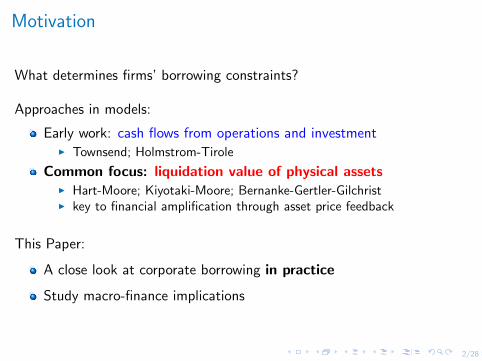
Motivation
What determines firms’ borrowing constraints?
Approaches in models:
Early work: cash flows from operations and investmentI Townsend; Holmstrom-Tirole
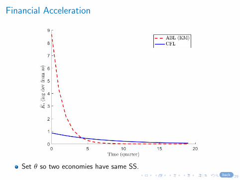
Common focus: liquidation value of physical assetsI Hart-Moore; Kiyotaki-Moore; Bernanke-Gertler-GilchristI key to financial amplification through asset price feedback
This Paper:
A close look at corporate borrowing in practice
Study macro-finance implications

Part 1. Corporate Borrowing in the US
1.1 Prevalence of “Cash Flow-Based Lending”
1.2 Prevalence of Earnings-Based Borrowing Constraints
1.3 Economic Foundations and Heterogeneity
3/28

4/28
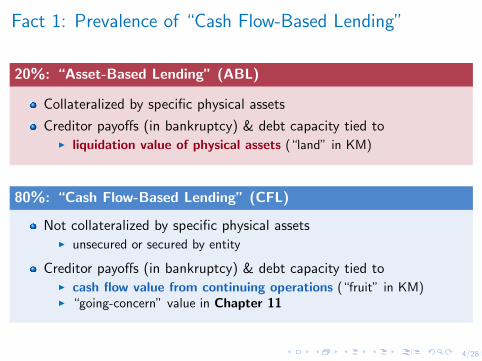
Fact 1: Prevalence of “Cash Flow-Based Lending”
20%: “Asset-Based Lending” (ABL)
Collateralized by specific physical assets
Creditor payoffs (in bankruptcy) & debt capacity tied toI liquidation value of physical assets (“land” in KM)
80%: “Cash Flow-Based Lending” (CFL)
Not collateralized by specific physical assetsI unsecured or secured by entity
Creditor payoffs (in bankruptcy) & debt capacity tied toI cash flow value from continuing operations (“fruit” in KM)I “going-concern” value in Chapter 11
4/28
Fact 1: Prevalence of “Cash Flow-Based Lending”
20%: “Asset-Based Lending” (ABL)
Collateralized by specific physical assets
Creditor payoffs (in bankruptcy) & debt capacity tied toI liquidation value of physical assets (“land” in KM)
80%: “Cash Flow-Based Lending” (CFL)
Not collateralized by specific physical assetsI unsecured or secured by entity
Creditor payoffs (in bankruptcy) & debt capacity tied toI cash flow value from continuing operations (“fruit” in KM)I “going-concern” value in Chapter 11

5/28
Fact 1: Prevalence of “Cash Flow-Based Lending”
Aggregate share by type :
Category Debt Type Share
Mortgages 6.5%Asset-based lending (20%)
Asset-based loans 13.5%Corporate bonds 48.0%
Cash flow-based lending (80%)Cash flow-based loans 32.0%
Firm-level median share by group (public firms):
Large Firms Rated Firms Small Firms
Asset-based lending 12.4% 8.0% 61.0%Cash flow-based lending 83.0% 89.0% 7.2%
large (assets>median): 96%+ debt, sales, capx, emp in all public firms
Integrate data from many sources: aggregate & debt level
FoF, FISD; DealScan, ABL Advisor, SNC, SDC; Call, SBA; Compustat; CapitalIQ

6/28
Fact 1: Prevalence of “Cash Flow-Based Lending”Similar in most industries
Median Share of Cash Flow-Based Lending: Rated Firms by Industry
All
NonDurables
Durables
Manufacturing
Mining/Refining
Chemicals
BusinessEquip
Telecom
Shops
HealthCare
Other
Utilities
Airlines
0 .2 .4 .6 .8 1Median Share of Cash Flow-Based Lending, Rated Firms

7/28
Fact 1: Prevalence of “Cash Flow-Based Lending”Composition stable over time
Composition of Debt: Public Firms Total0
.2.4
.6.8
1
2003 2005 2007 2009 2011 2013 2015Year
Share of Cash Flow-Based LendingShare of Asset-Based Lending

8/28
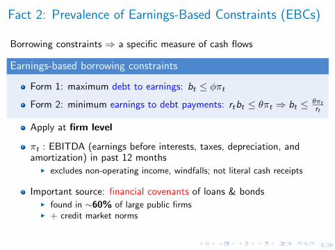
Fact 2: Prevalence of Earnings-Based Constraints (EBCs)
Borrowing constraints ⇒ a specific measure of cash flows
Earnings-based borrowing constraints
Form 1: maximum debt to earnings: bt ≤ φπtForm 2: minimum earnings to debt payments: rtbt ≤ θπt ⇒ bt ≤ θπt
rt
Apply at firm level
πt : EBITDA (earnings before interests, taxes, depreciation, andamortization) in past 12 months
I excludes non-operating income, windfalls; not literal cash receipts
Important source: financial covenants of loans & bondsI found in ∼60% of large public firmsI + credit market norms

8/28
Fact 2: Prevalence of Earnings-Based Constraints (EBCs)
Borrowing constraints ⇒ a specific measure of cash flows
Earnings-based borrowing constraints
Form 1: maximum debt to earnings: bt ≤ φπtForm 2: minimum earnings to debt payments: rtbt ≤ θπt ⇒ bt ≤ θπt
rt
Apply at firm level
πt : EBITDA (earnings before interests, taxes, depreciation, andamortization) in past 12 months
I excludes non-operating income, windfalls; not literal cash receipts
Important source: financial covenants of loans & bondsI found in ∼60% of large public firmsI + credit market norms

9/28
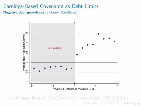
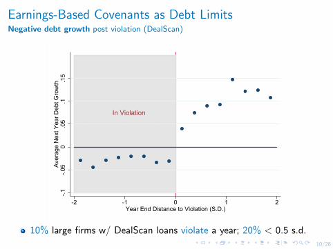
Earnings-Based Covenants
Financial covenants: legally binding provisionsI loans: assessed quarterly based on financial statementsI matter for both issuance and maintenance of debt
Covenant violation: technical defaultI creditors can accelerate paymentsI use it as threat → raise borrowing cost, charge fees, more restrictions
Effective debt limits: after violation of earnings-based covenantsI debt growth becomes negative on average
10/28
Earnings-Based Covenants as Debt LimitsNegative debt growth post violation (DealScan)
In Violation
-.1-.0
50
.05
.1.1
5Av
erag
e N
ext Y
ear D
ebt G
row
th
-2 -1 0 1 2Year End Distance to Violation (S.D.)
10% large firms w/ DealScan loans violate a year; 20% < 0.5 s.d.
10/28
Earnings-Based Covenants as Debt LimitsNegative debt growth post violation (DealScan)
In Violation
-.1-.0
50
.05
.1.1
5Av
erag
e N
ext Y
ear D
ebt G
row
th
-2 -1 0 1 2Year End Distance to Violation (S.D.)
10% large firms w/ DealScan loans violate a year; 20% < 0.5 s.d.

11/28
Earnings-Based Borrowing Constraints
“I think collateral is there mostly for some regulatory reasons.What banks really care is your EBITDA and coverage ratio.”
—Byron Pollitt, former CFO of Gap, Visa, Disney Parks & Resorts
Examples of firms w/ earnings-based covenants:
AAR Corp, AT&T, Barnes & Noble, Best Buy, Caterpillar, CBS Corp, Comcast,Costco, Disney, FedEx, GE, General Mills, Hershey’s, HP, IBM, Kohl’s, Lear Corp,Macy’s, Marriott, Merck, Northrop Grumman, Pfizer, Qualcomm, Rite Aid,Safeway, Sears, Sprint, Staples, Starbucks, Starwood Hotels, Target, TimeWarner, US Steel, Verizon, Whole Foods, Yum Brands...

12/28
Economic Foundations and Heterogeneity
Part 2. Financial Variables,Borrowing Constraints, Firm Outcomes
How do financial variables affect firms’borrowing constraints & outcomes on the margin?
2.1 Role of Cash Flows
2.2 Role of Physical Collateral Value
Firms are constrained, but a different type
13/28

Part 2. Financial Variables,Borrowing Constraints, Firm Outcomes
How do financial variables affect firms’borrowing constraints & outcomes on the margin?
2.1 Role of Cash Flows
2.2 Role of Physical Collateral Value
Firms are constrained, but a different type
13/28

14/28
Role of Cash Flows
Coty Inc[owner of fragrance brands Calvin Klein, Chloe, Davidoff, Marc Jacobs]
We remain dependent upon others for our financing needs, and our debtagreements contain restrictive covenants.
[F]inancial covenants restrict our operations and limit our flexibility andability to respond to changes or take certain actions.
Financial covenants...require us to maintain...a consolidated leverage ratioof total debt to EBITDA based on the previous 12-month period.

15/28
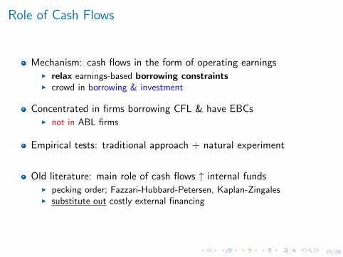
Role of Cash Flows
Mechanism: cash flows in the form of operating earningsI relax earnings-based borrowing constraintsI crowd in borrowing & investment
Concentrated in firms borrowing CFL & have EBCsI not in ABL firms
Empirical tests: traditional approach + natural experiment
Old literature: main role of cash flows ↑ internal fundsI pecking order; Fazzari-Hubbard-Petersen, Kaplan-ZingalesI substitute out costly external financing
15/28
Role of Cash Flows
Mechanism: cash flows in the form of operating earningsI relax earnings-based borrowing constraintsI crowd in borrowing & investment
Concentrated in firms borrowing CFL & have EBCsI not in ABL firms
Empirical tests: traditional approach + natural experiment
Old literature: main role of cash flows ↑ internal fundsI pecking order; Fazzari-Hubbard-Petersen, Kaplan-ZingalesI substitute out costly external financing

16/28
Traditional Approach: Sensitivity to EBITDA
Debt Issuance: Yit = αi + ηt + βEBITDAit + X ′itγ + εit-.2
-.10
.1.2
.3
Large w/ EBCs Large w/o EBCs Small Low Margin Air & Utilities
EBITDA
17/28
Additional Checks
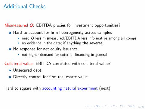
Mismeasured Q: EBITDA proxies for investment opportunities?
Hard to account for firm heterogeneity across samplesI need Q less mismeasured/EBITDA less informative among all compsI no evidence in the data; if anything the reverse
No response for net equity issuanceI not higher demand for external financing in general
Collateral value: EBITDA correlated with collateral value?
Unsecured debt
Directly control for firm real estate value
Hard to square with accounting natural experiment (next)
18/28
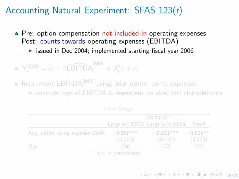
Accounting Natural Experiment: SFAS 123(r)
Pre: option compensation not included in operating expensesPost: counts towards operating expenses (EBITDA)
I issued in Dec 2004; implemented starting fiscal year 2006
Y 2006i = α + β EBITDA
2006
i + X ′i γ + εi
Instrument EBITDA2006i using prior option comp expenses
I controls: lags of EBITDA & dependent variable; firm characteristics
First Stage
EBITDA06i
Large w/ EBCs Large w/o EBCs Small
Avg. option comp expense 02-04 -0.857*** -0.721*** -0.520**(0.212) (0.134) (0.208)
Obs 686 435 727s.e. in parentheses

18/28
Accounting Natural Experiment: SFAS 123(r)
Pre: option compensation not included in operating expensesPost: counts towards operating expenses (EBITDA)
I issued in Dec 2004; implemented starting fiscal year 2006
Y 2006i = α + β EBITDA
2006
i + X ′i γ + εi
Instrument EBITDA2006i using prior option comp expenses
I controls: lags of EBITDA & dependent variable; firm characteristics
First Stage
EBITDA06i
Large w/ EBCs Large w/o EBCs Small
Avg. option comp expense 02-04 -0.857*** -0.721*** -0.520**(0.212) (0.134) (0.208)
Obs 686 435 727s.e. in parentheses
19/28
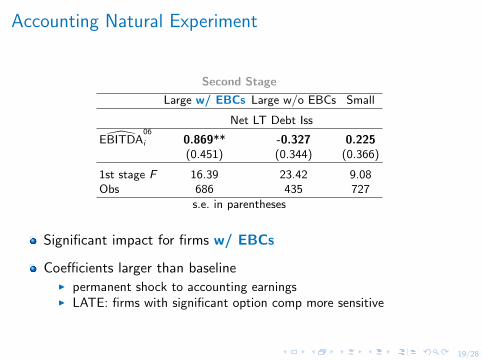
Accounting Natural Experiment
Second Stage
Large w/ EBCs Large w/o EBCs Small
Net LT Debt Iss
EBITDA06
i 0.869** -0.327 0.225(0.451) (0.344) (0.366)
1st stage F 16.39 23.42 9.08Obs 686 435 727
s.e. in parentheses
Significant impact for firms w/ EBCs
Coefficients larger than baselineI permanent shock to accounting earningsI LATE: firms with significant option comp more sensitive
How do financial variables affect firms’borrowing constraints & outcomes on the margin?
2.1 Role of Cash Flows
2.2 Role of Physical Collateral Value
Firms are constrained, but a different type
20/28

21/28
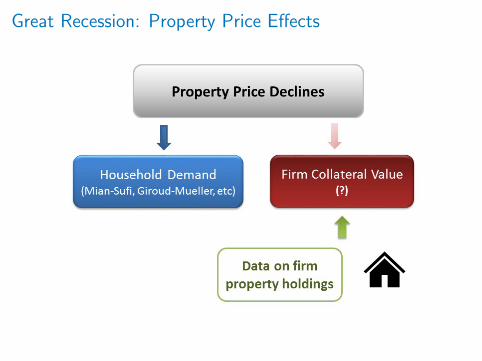
Role of Physical Collateral
For large firms which predominantly borrow CFL
Borrowing/investment sens. to collateral value (real estate) limitedI asset-based debt only
Great Recession: property price declinesI no significant collateral damage to major US non-financial firms
Financial acceleration among non-financial firmsI asset price feedback may dampen
22/28
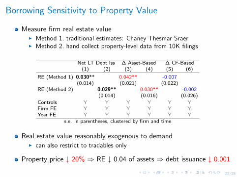
Borrowing Sensitivity to Property Value
Measure firm real estate valueI Method 1. traditional estimates: Chaney-Thesmar-SraerI Method 2. hand collect property-level data from 10K filings
Net LT Debt Iss ∆ Asset-Based ∆ CF-Based(1) (2) (3) (4) (5) (6)
RE (Method 1) 0.030** 0.042** -0.007(0.014) (0.021) (0.022)
RE (Method 2) 0.029** 0.030** -0.002(0.014) (0.016) (0.026)
Controls Y Y Y Y Y YFirm FE Y Y Y Y Y YYear FE Y Y Y Y Y Y
s.e. in parentheses, clustered by firm and time
Real estate value reasonably exogenous to demandI can also restrict to tradables only
Property price ↓ 20% ⇒ RE ↓ 0.04 of assets ⇒ debt issuance ↓ 0.001

23/28
Great Recession: Property Price Effects
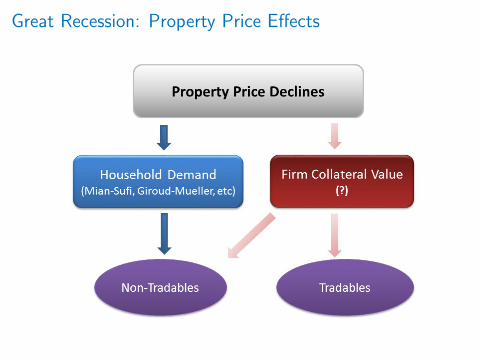
23/28
Great Recession: Property Price Effects
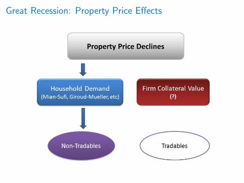
23/28
Great Recession: Property Price Effects
23/28
Great Recession: Property Price Effects

24/28
Great Recession: Property Price Effects
∆Y 07−09i = α + λ∆RE07−09
i ,06 + ηREi ,06 + φ∆P07−09i + X ′i γ + ui
I ∆RE07−09i,06 : change in market value of firm i ’s real estate 2007—2009
I based on properties owned by the end of 2006
Net LT Debt Issuance and Real Estate Value: 2007—2009
-.4-.2
0.2
Cha
nge
in N
et L
T D
ebt I
ssua
nce
07-0
9
-.15 -.1 -.05 0 .05Change in RE Value 07-09
Method 1
-.6-.4
-.20
.2C
hang
e in
Net
LT
Deb
t Iss
uanc
e 07
-09
-.15 -.1 -.05 0Change in RE Value 07-09
Method 2
25/28
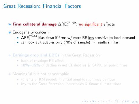
Great Recession: Financial Factors
Firm collateral damage ∆RE07−09i : no significant effects
Endogeneity concern:I ∆RE07−09
i bias down if firms w/ more RE less sensitive to local demandI can look at tradables only (70% of sample) ⇒ results similar
Earnings drop and EBCs in the Great RecessionI back-of-envelope PE effectI 10%∼15% of decline in net LT debt iss & CAPX, all public firms
Meaningful but not catastrophicI variants of KM model: financial amplification may dampenI key to the Great Recession: households & financial institutions

25/28
Great Recession: Financial Factors
Firm collateral damage ∆RE07−09i : no significant effects
Endogeneity concern:I ∆RE07−09
i bias down if firms w/ more RE less sensitive to local demandI can look at tradables only (70% of sample) ⇒ results similar
Earnings drop and EBCs in the Great RecessionI back-of-envelope PE effectI 10%∼15% of decline in net LT debt iss & CAPX, all public firms
Meaningful but not catastrophicI variants of KM model: financial amplification may dampenI key to the Great Recession: households & financial institutions

US vs. Japan
Take nothing for granted
26/28
27/28
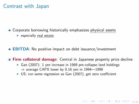
Contrast with Japan
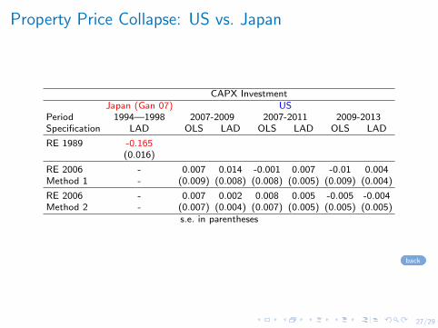
Corporate borrowing historically emphasizes physical assetsI especially real estate
EBITDA: No positive impact on debt issuance/investment
Firm collateral damage: Central in Japanese property price declineI Gan (2007): 1 yen increase in 1989 pre-collapse land holdings⇒ average CAPX lower by 0.16 yen in 1994—1998
I US: run same regression as Gan (2007), get zero coefficient
28/28
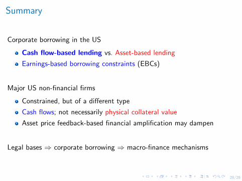
Summary
Corporate borrowing in the US
Cash flow-based lending vs. Asset-based lending
Earnings-based borrowing constraints (EBCs)
Major US non-financial firms
Constrained, but of a different type
Cash flows; not necessarily physical collateral value
Asset price feedback-based financial amplification may dampen
Legal bases ⇒ corporate borrowing ⇒ macro-finance mechanisms

Thank You
28/28
1/29
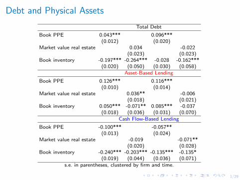
Debt and Physical Assets
Total Debt
Book PPE 0.043*** 0.096***(0.012) (0.020)
Market value real estate 0.034 -0.022(0.023) (0.023)
Book inventory -0.197*** -0.264*** -0.028 -0.162***(0.020) (0.050) (0.030) (0.058)
Asset-Based Lending
Book PPE 0.126*** 0.116***(0.010) (0.014)
Market value real estate 0.036** -0.006(0.018) (0.021)
Book inventory 0.050*** -0.071** 0.085*** -0.037(0.018) (0.036) (0.031) (0.070)
Cash Flow-Based Lending
Book PPE -0.100*** -0.057**(0.013) (0.024)
Market value real estate -0.019 -0.071**(0.020) (0.028)
Book inventory -0.240*** -0.203*** -0.135*** -0.135*(0.019) (0.044) (0.036) (0.071)
s.e. in parentheses, clustered by firm and time.
2/29
Debt and Physical Assets (more)
Mortgage
Book PPE 0.038*** 0.022***(0.003) (0.003)
Market value real estate 0.017*** 0.019***(0.004) (0.006)
Book inventory 0.003 0.009 0.003 -0.020(0.003) (0.008) (0.004) (0.017)
Non-Mortgage ABL
Book PPE 0.066*** 0.081***(0.009) (0.013)
Market value real estate 0.007 -0.026(0.017) (0.021)
Book inventory 0.055*** -0.056* 0.082*** -0.011(0.016) (0.032) (0.029) (0.070)
Cash Flow-Based Loans
Book PPE -0.055*** -0.026**(0.009) (0.010)
Market value real estate -0.021** -0.002(0.010) (0.019)
Book inventory -0.089*** -0.096*** -0.051*** 0.004(0.011) (0.023) (0.014) (0.041)
s.e. in parentheses, s.e. clustered by firm and time.
back

3/29
Prevalence of Cash Flow-Based Lending
Composition of Debt: Large Firm Median
0.2
.4.6
.81
2003 2005 2007 2009 2011 2013 2015Year
Share of Cash Flow-Based LendingShare of Asset-Based Lending
back

4/29
Prevalence of EBCs: Large US Firms
Fraction w/ Earnings-Based Covenants: Large Public Firms
0.2
.4.6
.81
Frac
tion
with
EBC
s
1997 2000 2003 2006 2009 2012 2015Year
back

5/29
Bunching around Earnings-Based Covenant Threshold
0.2
.4.6
.8D
ensi
ty
-2 -1 0 1 2S.D. to Violation
back

6/29
Timeline
Single covenant: issuance + maintenance
T0
borrow Debt0
b0 ≤ θ0π0
T1
b1 ≤ θ0π1
T2
b2 ≤ θ0π2
Multiple covenants: tightest one binds first
T0
borrow Debt0
b0 ≤ θ0π0
T1
b1 ≤ θ0π1
T2
borrow Debt1
b2 ≤ min{θ0, θ1}π2
T3
Debt0 matures
borrow Debt2
D3 ≤ min{θ1, θ2}π3
back

7/29
Other Forms of Financial Covenants
Main alternative: covenants on book leverage/book net worthI not market net worthI book net worth (i.e. book equity) ≈ accumulation of past earningsI cousin of earnings-based covenants
Prevalence:I ∼20% large public firmsI declining substantially over time
Tightness:I less constrainingI less than 2% of large public firms w/ bank loans violate in a given year
back

8/29
Other Forms of Financial Covenants
Financial Covenants among Large Public Firms0
.25
.5.7
5
1997 2000 2003 2006 2009 2012 2015Year
Firms w/ Earnings-Based CovenantsFirms w/ Book Leverage or Net Worth CovenantsFirms w/ Liquidity Covenants
9/29
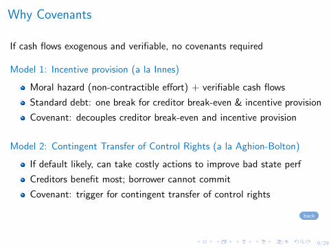
Why Covenants
If cash flows exogenous and verifiable, no covenants required
Model 1: Incentive provision (a la Innes)
Moral hazard (non-contractible effort) + verifiable cash flows
Standard debt: one break for creditor break-even & incentive provision
Covenant: decouples creditor break-even and incentive provision
Model 2: Contingent Transfer of Control Rights (a la Aghion-Bolton)
If default likely, can take costly actions to improve bad state perf
Creditors benefit most; borrower cannot commit
Covenant: trigger for contingent transfer of control rights
back
10/29
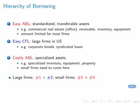
Hierarchy of Borrowing
1 Easy ABL: standardized, transferable assetsI e.g. commercial real estate (office), receivable, inventory, equipmentI amount limited for most firms
2 Easy CFL: large firms in USI e.g. corporate bonds, syndicated loans
3 Costly ABL: specialized assetsI e.g. specialized inventory, equipment, propertyI small firms need to come here
Large firms: #1 + #2; small firms: #1 + #3
back
11/29
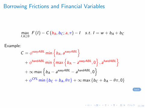
Borrowing Frictions and Financial Variables
maxI ,b≥0
F (I )− C (bA, bC ; a, π)− I s.t. I = w + bA + bC
Example:
C = φeasyABL min{bA, a
easyABL}
+ φhardABL min{
max{bA − aeasyABL, 0
}, ahardABL
}+∞max
{bA − aeasyABL − ahardABL, 0
}+ φCFL min {bC + bA, θπ}+∞max {bC + bA − θπ, 0}
back
12/29
Traditional Approach: Sensitivity to EBITDA
Debt Issuance: Yit = αi + ηt + βEBITDAit + κOCFit + X ′itγ + εit-.2
0.2
.4
Large w/ EBCs Large w/o EBCs Small Low Margin Air & Utilities
EBITDA OCF

13/29
Traditional Approach: Sensitivity to EBITDA
CAPX Investment: Yit = αi + ηt + βEBITDAit + κOCFit + X ′itγ + εit-.1
0.1
.2.3
Large w/ EBCs Large w/o EBCs Small Low Margin Air & Utilities
EBITDA OCF
back
14/29
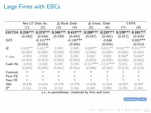
Large Firms with EBCs
Net LT Debt Iss. ∆ Book Debt ∆ Unsec. Debt CAPX(1) (2) (3) (4) (5) (6) (7) (8)
EBITDA 0.216*** 0.273*** 0.345*** 0.412*** 0.209*** 0.232*** 0.129*** 0.101***(0.030) (0.034) (0.039) (0.042) (0.037) (0.041) (0.017) (0.019)
OCF -0.111*** -0.135*** -0.048 0.053***(0.033) (0.045) (0.033) (0.013)
Q 0.010** 0.011** 0.004 0.005 0.010** 0.011** 0.011*** 0.011***(0.005) (0.005) (0.005) (0.005) (0.004) (0.004) (0.002) (0.002)
r−12m -0.003 -0.003 0.002 0.001 0.002 0.002 0.004* 0.004*(0.003) (0.003) (0.003) (0.003) (0.003) (0.003) (0.002) (0.002)
Cash Ho -0.033 -0.033 0.039 0.039 -0.117*** -0.117*** 0.015 0.015(0.043) (0.044) (0.051) (0.052) (0.044) (0.043) (0.013) (0.013)
Controls Y Y Y Y Y Y Y YFirm FE Y Y Y Y Y Y Y YYear FE Y Y Y Y Y Y Y YObs 15,642 15,642 15,576 15,576 11,693 11,693 16,907 16,907R2 0.114 0.116 0.152 0.154 0.069 0.069 0.156 0.160
s.e. in parentheses, clustered by firm and time
accounting coef
15/29
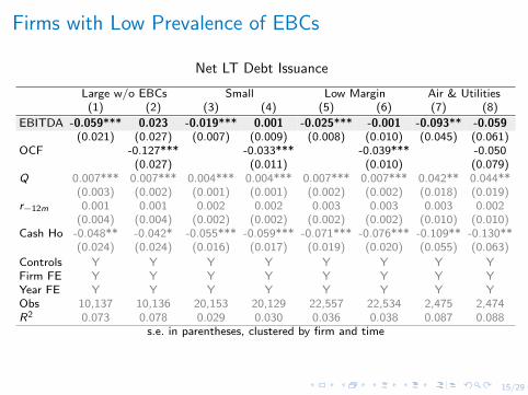
Firms with Low Prevalence of EBCs
Net LT Debt Issuance
Large w/o EBCs Small Low Margin Air & Utilities(1) (2) (3) (4) (5) (6) (7) (8)
EBITDA -0.059*** 0.023 -0.019*** 0.001 -0.025*** -0.001 -0.093** -0.059(0.021) (0.027) (0.007) (0.009) (0.008) (0.010) (0.045) (0.061)
OCF -0.127*** -0.033*** -0.039*** -0.050(0.027) (0.011) (0.010) (0.079)
Q 0.007*** 0.007*** 0.004*** 0.004*** 0.007*** 0.007*** 0.042** 0.044**(0.003) (0.002) (0.001) (0.001) (0.002) (0.002) (0.018) (0.019)
r−12m 0.001 0.001 0.002 0.002 0.003 0.003 0.003 0.002(0.004) (0.004) (0.002) (0.002) (0.002) (0.002) (0.010) (0.010)
Cash Ho -0.048** -0.042* -0.055*** -0.059*** -0.071*** -0.076*** -0.109** -0.130**(0.024) (0.024) (0.016) (0.017) (0.019) (0.020) (0.055) (0.063)
Controls Y Y Y Y Y Y Y YFirm FE Y Y Y Y Y Y Y YYear FE Y Y Y Y Y Y Y YObs 10,137 10,136 20,153 20,129 22,557 22,534 2,475 2,474R2 0.073 0.078 0.029 0.030 0.036 0.038 0.087 0.088
s.e. in parentheses, clustered by firm and time
16/29
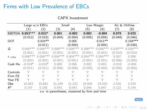
Firms with Low Prevalence of EBCs
CAPX Investment
Large w/o EBCs Small Low Margin Air & Utilities(1) (2) (3) (4) (5) (6) (7) (8)
EBITDA 0.053*** 0.033* 0.001 -0.002 0.002 -0.004 0.079 0.025(0.012) (0.019) (0.004) (0.004) (0.005) (0.004) (0.049) (0.046)
OCF 0.024** 0.005 0.011** 0.158***(0.011) (0.004) (0.005) (0.038)
Q 0.004*** 0.004*** 0.006*** 0.006*** 0.006*** 0.006*** 0.029*** 0.026***(0.001) (0.001) (0.001) (0.001) (0.001) (0.001) (0.010) (0.010)
r−12m 0.006*** 0.006*** 0.004*** 0.004*** 0.004*** 0.004*** 0.007 0.006(0.002) (0.002) (0.001) (0.001) (0.001) (0.001) (0.006) (0.006)
Cash Ho -0.019* -0.019* 0.005 0.006 0.002 0.003 -0.018 -0.004(0.011) (0.011) (0.006) (0.006) (0.005) (0.005) (0.056) (0.056)
Controls Y Y Y Y Y Y Y YFirm FE Y Y Y Y Y Y Y YYear FE Y Y Y Y Y Y Y YObs 10,683 10,681 21,249 21,222 24,045 24,020 2,535 2,534R2 0.107 0.108 0.043 0.043 0.046 0.047 0.122 0.144
s.e. in parentheses, clustered by firm and time
back

17/29
Accounting Relationships
EBITDA = SALE− COGS−XSGA
OCF = EBITDA+ (NOPI + SPI) + SPPE︸ ︷︷ ︸non-operating & other income
− (TAX−DTAX−∆ATAX)︸ ︷︷ ︸cash taxes paid
+∆AP−∆AR−∆INV + ∆UR−∆PX + OCFO︸ ︷︷ ︸difference between earnings & cash receipts
NOPI: non-operating income; SPI: special items; SPPE: sale of PPE;
TAX: income taxes; DTAX: deferred taxes; ATAX: accrued taxes;
UR: unearned revenue, PX: prepaid expenses.
Differences between EBITDA and OCF
Timing of earnings recognition vs. cash paymentI does not affect EBITDA; does affect OCF
Non-operating & other incomeI does not affect EBITDA; does affect OCF
back
18/29
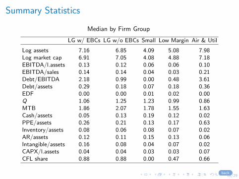
Summary Statistics
Median by Firm Group
LG w/ EBCs LG w/o EBCs Small Low Margin Air & Util
Log assets 7.16 6.85 4.09 5.08 7.98Log market cap 6.91 7.05 4.08 4.88 7.18EBITDA/l.assets 0.13 0.12 0.06 0.06 0.10EBITDA/sales 0.14 0.14 0.04 0.03 0.21Debt/EBITDA 2.18 0.99 0.00 0.48 3.61Debt/assets 0.29 0.18 0.07 0.18 0.36EDF 0.00 0.00 0.01 0.02 0.00Q 1.06 1.25 1.23 0.99 0.86MTB 1.86 2.07 1.78 1.55 1.63Cash/assets 0.05 0.13 0.19 0.12 0.02PPE/assets 0.26 0.21 0.13 0.17 0.63Inventory/assets 0.08 0.06 0.08 0.07 0.02AR/assets 0.12 0.11 0.15 0.13 0.06Intangible/assets 0.16 0.08 0.04 0.07 0.02CAPX/l.assets 0.04 0.04 0.03 0.03 0.07CFL share 0.88 0.88 0.00 0.47 0.66
back

19/29
Predicting Future EBITDA
Yit+k = αi + ηt + βEBITDAit + κOCF + X ′itγ + εit0
.1.2
.3.4
.5
Large w/ EBCs Large w/o EBCs Small Low Margin Air & Utilities
EBITDA t+1 EBITDA t+2back

20/29
Controlling for Real Estate Value
Net LT Debt Iss CAPX(1) (2) (3) (4)
EBITDA 0.325*** 0.330*** 0.077*** 0.082***(0.064) (0.066) (0.022) (0.022)
OCF -0.135*** -0.134*** 0.018 0.019(0.037) (0.037) (0.015) (0.015)
Q 0.006 0.007 0.013*** 0.013***(0.006) (0.006) (0.004) (0.004)
Past 12m stock ret -0.004 -0.005 0.002 0.002(0.006) (0.006) (0.002) (0.002)
Cash Ho -0.036 -0.037 0.016 0.015(0.067) (0.066) (0.015) (0.016)
RE 0.035* 0.036***(0.018) (0.009)
Controls Y Y Y YFirm FE Y Y Y YYear FE Y Y Y YObs 4,554 4,554 4,540 4,540R2 0.116 0.116 0.186 0.194
Standard errors in parentheses, clustered by firm and time*** p<0.01, ** p<0.05, * p<0.1
back
21/29
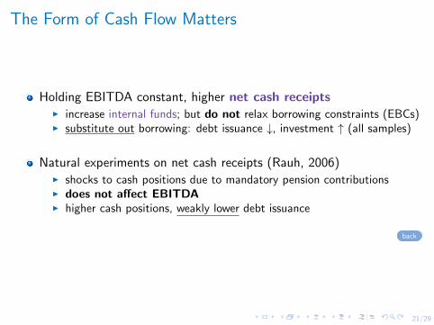
The Form of Cash Flow Matters
Holding EBITDA constant, higher net cash receiptsI increase internal funds; but do not relax borrowing constraints (EBCs)I substitute out borrowing: debt issuance ↓, investment ↑ (all samples)
Natural experiments on net cash receipts (Rauh, 2006)I shocks to cash positions due to mandatory pension contributionsI does not affect EBITDAI higher cash positions, weakly lower debt issuance
back
22/29
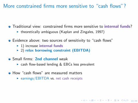
More constrained firms more sensitive to “cash flows”?
Traditional view: constrained firms more sensitive to internal funds?I theoretically ambiguous (Kaplan and Zingales, 1997)
Evidence above: two sources of sensitivity to “cash flows”I 1) increase internal fundsI 2) relax borrowing constraint (EBITDA)
Small firms: 2nd channel weakI cash flow-based lending & EBCs less prevalent
How “cash flows” are measured mattersI earnings/EBITDA vs. net cash receipts

23/29
More constrained firms more sensitive to “cash flows”?Large vs. Small Firms
Net LT Debt Iss CAPXLarge Firm Small Firm Large Firm Small Firm
EBITDA 0.092*** 0.173*** -0.019*** 0.001 0.099*** 0.078*** 0.001 -0.002(0.020) (0.023) (0.007) (0.009) (0.011) (0.012) (0.004) (0.004)
OCF -0.141*** -0.033*** 0.038*** 0.005(0.022) (0.011) (0.008) (0.004)
Q 0.007*** 0.007*** 0.004*** 0.004*** 0.006*** 0.006*** 0.006*** 0.006***(0.002) (0.002) (0.001) (0.001) (0.001) (0.001) (0.001) (0.001)
r−12m 0.001 0.000 0.002 0.002 0.005*** 0.005*** 0.004*** 0.004***(0.003) (0.003) (0.002) (0.002) (0.002) (0.002) (0.001) (0.001)
Cash Ho -0.027 -0.026 -0.055*** -0.059*** 0.013* 0.014* 0.005 0.006(0.020) (0.021) (0.016) (0.017) (0.007) (0.008) (0.006) (0.006)
Controls Y Y Y Y Y Y Y YFirm FE Y Y Y Y Y Y Y YYear FE Y Y Y Y Y Y Y YObs 26,165 26,164 20,153 20,129 27,982 27,980 21,249 21,222R2 0.076 0.080 0.029 0.030 0.129 0.131 0.043 0.043
s.e. in parentheses, clustered by firm and time
back
24/29
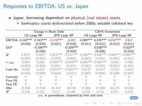
Responses to EBITDA: US vs. Japan
Japan: borrowing dependent on physical (real estate) assetsI bankruptcy courts dysfunctional before 2000s; seizable collateral key
Change in Book Debt CAPX InvestmentUS Large NF JPN Large NF US Large NF JPN Large NF
EBITDA 0.160*** 0.283*** -0.178*** -0.022 0.099*** 0.078*** 0.037*** 0.017(0.028) (0.025) (0.021) (0.016) (0.011) (0.012) (0.012) (0.011)
OCF -0.194*** -0.329*** 0.038*** 0.020**(0.030) (0.020) (0.008) (0.010)
Q 0.003* 0.003* 0.013*** 0.011*** 0.006*** 0.006*** 0.008*** 0.008***(0.002) (0.002) (0.003) (0.003) (0.001) (0.001) (0.001) (0.001)
r−12m 0.003 0.003 -0.004*** -0.004*** 0.005*** 0.005*** -0.001 -0.001(0.003) (0.003) (0.001) (0.001) (0.002) (0.002) (0.001) (0.001)
Cash Ho 0.020 0.023 -0.072*** -0.081*** 0.013* 0.014* -0.012 -0.012(0.028) (0.028) (0.016) (0.017) (0.007) (0.008) (0.008) (0.007)
Controls Y Y Y Y Y Y Y YFirm FE Y Y Y Y Y Y Y YYear FE Y Y Y Y Y Y Y YObs 27,936 27,919 20,422 20,338 27,982 27,980 20,176 20,086R2 0.116 0.123 0.112 0.169 0.129 0.131 0.071 0.070
s.e. in parentheses, clustered by firm and timeback
25/29
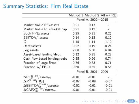
Summary Statistics: Firm Real Estate
Method 1 Method 2 All w/ RE
Panel A. 2002—2015
Market Value RE/assets 0.21 0.13 -Market Value RE/market cap 0.21 0.12 -Book PPE/assets 0.25 0.21 0.25EBITDA/l.assets 0.14 0.13 0.12Q 1.15 1.14 1.10Debt/assets 0.22 0.19 0.24Log assets 7.08 6.30 6.84Asset-based lending/debt 0.12 0.25 0.22Cash flow-based lending/debt 0.85 0.66 0.74Fraction of large firms 0.76 0.63 0.71Fraction w/ EBCs 0.60 0.55 0.56
Panel B. 2007—2009
∆RE07−0906 /assets06 -0.01 -0.01 -
∆P07−09(HQ) -0.07 -0.08 -0.07∆EBITDA07−09
06 /assets06 -0.02 -0.01 -0.01∆CAPX07−09
06 /assets06 -0.01 -0.01 -0.01
back

26/29
Borrowing Sensitivity to Property Value: Tradables Only
Net LT Debt Iss ∆ Asset-Based ∆ CF-Based(1) (2) (3) (4) (5) (6)
RE (Method 1) 0.024 0.060** -0.090***(0.031) (0.030) (0.027)
RE (Method 2) 0.063** 0.075* -0.003(0.031) (0.040) (0.022)
EBITDA 0.182*** 0.136*** 0.119*** 0.065** 0.121* 0.109**(0.055) (0.043) (0.046) (0.033) (0.071) (0.050)
OCF -0.155*** -0.170*** -0.109*** -0.141*** -0.097** -0.089*(0.035) (0.045) (0.039) (0.035) (0.047) (0.048)
Q 0.006 0.016** -0.005* 0.003 0.002 0.013(0.005) (0.007) (0.003) (0.003) (0.008) (0.008)
Cash Ho -0.047 -0.074*** -0.081*** -0.063** 0.040 -0.020(0.038) (0.027) (0.030) (0.029) (0.040) (0.036)
Controls Y Y Y Y Y YFirm FE Y Y Y Y Y YYear FE Y Y Y Y Y YObs 3,174 2,820 3,174 2,820 3,174 2,820R2 0.111 0.122 0.212 0.234 0.211 0.195
s.e. in parentheses, clustered by firm and time
back
27/29
Property Price Collapse: US vs. Japan
CAPX InvestmentJapan (Gan 07) US
Period 1994—1998 2007-2009 2007-2011 2009-2013Specification LAD OLS LAD OLS LAD OLS LAD
RE 1989 -0.165(0.016)
RE 2006 - 0.007 0.014 -0.001 0.007 -0.01 0.004Method 1 - (0.009) (0.008) (0.008) (0.005) (0.009) (0.004)
RE 2006 - 0.007 0.002 0.008 0.005 -0.005 -0.004Method 2 - (0.007) (0.004) (0.007) (0.005) (0.005) (0.005)
s.e. in parentheses
back
28/29
Financial Acceleration
Set θ so two economies have same SS.back