lable at ScienceDirect

Hearing Research 382 (2019) 107779

Contents lists avai

Hearing Research

journal homepage: www.elsevier .com/locate/heares

Research Paper

Analyzing the FFR: A tutorial for decoding the richness of auditoryfunction

Jennifer Krizman a, Nina Kraus a, b, *

a Auditory Neuroscience Laboratory, Department of Communication Sciences and Disorders, Northwestern University, Evanston, IL, 60208, USAb Department of Neurobiology, Northwestern University, Evanston, IL, 60208, USA

a r t i c l e i n f o

Article history:Received 6 July 2019Received in revised form1 August 2019Accepted 6 August 2019Available online 8 August 2019

Outline

1 Introduction1.1 What is the FFR?1.2 Purpose of this tutorial

2 FFR Components2.1 Timing2.2 Fundamental frequency (F0)2.3 Harmonics2.4 Non-stimulus activity

3 Factors Influencing the FFR3.1 Stimulus polarity3.2 Averaging versus single trial3.3 Stimulus presentation timing

4 Analyzing the FFR4.1 Overview4.2 Timing4.2.1 Peak picking4.2.2 Frequency-specific

* Corresponding author. Northwestern University, 2IL, 60208, USA.

E-mail address: nkraus@northwestern.edu (N. KraURL: https://www.brainvolts.northwestern.edu

https://doi.org/10.1016/j.heares.2019.1077790378-5955/© 2019 Elsevier B.V. All rights reserved.

a b s t r a c t

The frequency-following response, or FFR, is a neurophysiological response to sound that precisely re-flects the ongoing dynamics of sound. It can be used to study the integrity and malleability of neuralencoding of sound across the lifespan. Sound processing in the brain can be impaired with pathology andenhanced through expertise. The FFR can index linguistic deprivation, autism, concussion, and readingimpairment, and can reflect the impact of enrichment with short-term training, bilingualism, andmusicianship. Because of this vast potential, interest in the FFR has grown considerably in the decadesince our first tutorial. Despite its widespread adoption, there remains a gap in the current knowledge ofits analytical potential. This tutorial aims to bridge this gap. Using recording methods we have employedfor the last 20 þ years, we have explored many analysis strategies. In this tutorial, we review what wehave learned and what we think constitutes the most effective ways of capturing what the FFR can tell us.The tutorial covers FFR components (timing, fundamental frequency, harmonics) and factors that in-fluence FFR (stimulus polarity, response averaging, and stimulus presentation/recording jitter). Thespotlight is on FFR analyses, including ways to analyze FFR timing (peaks, autocorrelation, phase con-sistency, cross-phaseogram), magnitude (RMS, SNR, FFT), and fidelity (stimulus-response correlations,response-to-response correlations and response consistency). The wealth of information containedwithin an FFR recording brings us closer to understanding how the brain reconstructs our sonic world.

© 2019 Elsevier B.V. All rights reserved.

(continued )

Outline

4.2.2.1 Autocorrelation4.2.2.2 Phase consistency4.2.2.3 Cross-phaseogram

4.3 Magnitude4.3.1 Broadband4.3.1.1 RMS and SNR

4.3.2 Frequency-specific4.3.2.1 Fast-Fourier transform

4.4 Fidelity4.4.1 Stimulus-to-response correlation4.4.2 Response-to-response correlation4.4.3 Response consistency

5 Other Considerations5.1 Different recording methods5.2 Click-ABR

6 Summary and Conclusions7 References

240 Campus Drive, Evanston,

us).

J. Krizman, N. Kraus / Hearing Research 382 (2019) 1077792

1. Introduction

1.1. What is the FFR?

The frequency-following response, or FFR, is a neurophysiolog-ical response to sound that reflects the neural processing of asound's acoustic features with uncommon precision.

These scalp-recorded potentials to speech have been recorded inhumans for the past 25 þ years (Galbraith et al., 1995, 1997, 1998;Krishnan, 2002; Krishnan and Gandour, 2009; Krishnan et al., 2004;Russo et al., 2004) and FFRs can be recorded across the lifespan frominfants through older adults (Jeng et al., 2011; Ribas-Prats et al.,2019; Skoe et al., 2015). By virtue of being generated predomi-nately in the auditory midbrain (Bidelman, 2015; Chandrasekaranand Kraus, 2010; Sohmer et al., 1977; White-Schwoch et al.,2016b; White-Schwoch et al., in press), a hub of afferent andefferent activity (Malmierca, 2015; Malmierca and Ryugo, 2011), theFFR reflects an array of influences from the auditory periphery andthe central nervous system. The FFR can provide a measure of brainhealth, as it can index linguistic deprivation (Krizman et al., 2016;Skoe et al., 2013a), autism (Chen et al., 2019; Otto-Meyer et al., 2018;Russo et al., 2008), concussion (Kraus et al., 2016a, 2016b, 2017b;Vander Werff and Rieger, 2017), hyperbilirubinemia in infants(Musacchia et al., 2019), and learning or reading impairments (Banaiet al., 2009; Hornickel and Kraus, 2013; Hornickel et al., 2009; Neefet al., 2017; White-Schwoch et al., 2015). The FFR has provenessential to answering basic questions about how our auditorysystem manages complex acoustic information and how it in-tegrates with other senses (Anderson et al., 2010a, 2010b;Musacchia et al., 2007; Selinger et al., 2016). It can reveal auditorysystemplasticity over short timescales (Skoe andKraus, 2010b; Songet al., 2008) or lifelong experience, such as speaking a tonal language(Jeng et al., 2011; Krishnan et al., 2005), bilingualism (Krizman et al.,2012b, 2014, 2015, 2016; Omote et al., 2017; Skoe et al., 2017) ormusicianship (reviewed in Kraus and White-Schwoch, 2017;Parbery-Clark et al., 2009; Strait et al., 2009; Strait et al., 2013;Tierney et al., 2015; Tierney et al., 2013; Wong et al., 2007).

1.2. Purpose of this tutorial

This tutorial is not a review of the FFR's history, origins,experience-dependence, nor its many applications, as those topicshave been dealt with in detail elsewhere (Kraus &White-Schwoch,2015, 2017; Kraus et al., 2017a). How to record the response is wellunderstood. There remains, however, a major gap in the currentknowledge of how to analyze this rich response. Therefore, in thistutorial, we focus on data analyses. We touch on data collectionparameters, but only insomuch as they affect FFR analyses. We aimto help clinicians and researchers understand the considerationsthat go into determining a protocol, based on the question at handand the type of analyses best suited for that question, as thereappears to be an interest in this within the field (e.g., BinKhamiset al., 2019; Sanfins et al., 2018). We provide an overview of thetypes of analyses that are appropriate for investigating the multi-faceted layers of auditory processing present in the FFR and howsome of that richness can be obscured or lost depending on how thedata are collected. This tutorial is focused on the FFR we are mostfamiliar with and the technique employed in our lab: a midline-vertex (i.e., Cz) scalp recording of an evoked response to speech,music, or environmental sounds (Fig. 1). We originally chose thisrecording site to align the electrode with the inferior colliculus tomaximize the capture of activity from subcortical FFR generators.We continue recording from here because we have developed anormative database over the years of FFRs recorded at this site tomany different stimuli in thousands of individuals, many

longitudinally, across a wide range of participant demographics(Kraus and Chandrasekaran, 2010; Kraus & White-Schwoch, 2015,2017; Krizman et al., 2019; Russo et al., 2004; Skoe and Kraus,2010a; Skoe et al., 2015). In the ten years since our first tutorial(Skoe and Kraus, 2010a), we have employed many analysis tech-niques and what follows is a review of what we have learned andwhat we think constitutes the most effective ways of capturingwhat the FFR can tell us.

2. FFR components

The FFR provides considerable detail about sound processing inthe brain. When talking about the FFR, we like to use a mixingboard analogy, as each component of the FFR distinctly contributesto the gestalt, with each telling us something about sound pro-cessing. This processing of sound details distinguishes FFR fromother evoked responses. When recording FFR to a complex sound,like speech or music, we typically consider three overarching fea-tures of the response: timing, fundamental frequency, and har-monics. We also consider the accompanying non-stimulus-evokedactivity. Each of these components contains awealth of information(described in the data analyses section).

2.1. Timing

Amplitude deflections in the signal act as landmarks that arereflected in the response (Fig. 1). These peaks occur at a specifictime in the signal and should therefore occur at a correspondingtime in the response. Generally, peaks fall into two categories. Oneis in response to a stimulus change, such as an onset, offset, ortransition (e.g., onset to steady-state transition) while the othercategory reflects the periodicity of the stimulus. A term used todefine a peak's timing in the response is latency, which is refer-enced to stimulus onset, or less frequently, to an acoustic eventlater in the stimulus. One may also evaluate relative timing of peakswithin a response or of peaks between two responses (e.g., to thesame stimulus presented in quiet v. background noise). In additionto looking at timing via peaks in the time-domain response, one canlook at the phase of individual frequencies within the response.

2.2. Fundamental frequency

The fundamental frequency (F0) is by definition the lowestfrequency of a periodic waveform and therefore corresponds to theperiodicity of the sound, or repetition rate of the sound envelope.For a speech sound, this corresponds to the rate at which the vocalfolds vibrate. In music, the fundamental is the frequency of thelowest perceived pitch of a given note. The neural response to theF0 is rich in and of itself. We have a number of methods forextracting information about the phase, encoding strength, andperiodicity of the F0 (Table 1).

2.3. Harmonics

Harmonics are integer multiples of the F0. Typically all har-monics present in the stimulus are present in the FFR, at least up toabout 1.2e1.3 kHz (Chandrasekaran and Kraus, 2010) and the ceil-ing frequency varies depending on whether you are looking at theresponse to a single stimulus polarity, or the added, or subtractedresponse to opposing-polarity stimuli (see Stimulus Polarity, below,and Figs. 2 and 3). Non-linearities of the auditory system canintroduce harmonic peaks in the FFR outside those present in thestimulus or at different strengths than one would predict from thestimulus composition (Warrier et al., 2011). In a speech stimulus,certain harmonics, called formants, are of particular importance

Fig. 1. The FFR reflects transient and sustained features of the evoking stimulus. We have used a variety of stimuli to record FFRs. A few shown here include triangle waves of asingle frequency (the notes C4 and G4), the notes G2 and E3 making a major 6th chord (chord), speech syllables with a flat (ba, ta) or a changing (falling ya) pitch, environmentalsounds, like the bowing of a cello, a burp, or a baby's cry. From the time domain FFRs on the right, it is evident that they contain much of the information found in the stimulus (leftpanel). The increase in frequency from C4 (262 Hz) to G4 (392 Hz) is mirrored in the FFR as is the later voice-onset time for ‘ta’ versus ‘ba’ and the falling frequency for the ‘ya’ from320 to 130 Hz can be seen by the greater spacing of FFR peaks corresponding to the falling pitch.

J. Krizman, N. Kraus / Hearing Research 382 (2019) 107779 3

phonetically and are somewhat independent of the F0 of the speechsound. Formants are harmonics that are larger in amplitude thansurrounding harmonics, both in the stimulus and in the FFR. Forexample, the first formant of /a/corresponds to a local peak at~700e750Hz, while /i/, will have a first formant in the 250e300 Hzrange, regardless of the F0 of the utterance.

2.4. Non-stimulus activity

The stimulus used to evoke an FFR is presented multiple timesand there is a gap of silence between each stimulus presentation.We measure the amount of neural activity that occurs during thissilent interval to provide us with information about the neuralactivity that is not time-locked to the stimulus, which can be callednon-stimulus activity, prestimulus activity, or neural noise.

3. Factors influencing the FFR

3.1. Stimulus polarity

In the cochlea, a periodic sound, such as a sine wave, will open

ion channels on the hair cell stereocilia in one-half of its cycle, andclose the channels during the other-half of its cycle, a processknown as half-wave rectification. Additionally, the tonotopicarrangement of the cochlea causes earlier activation of auditorynerve fibers that respond to higher frequencies at the basal end ofthe cochlea compared to the nerve fibers that respond to lowerfrequencies at the apex (Greenberg et al., 1998; Greenwood, 1961;Ruggero and Rich, 1987). Consequently, the timing of auditorynerve responses will differ depending on whether they receiveinformation from more basal or apical areas of the cochlea orwhether the initial deflection of the stereocilia is hyperpolarizing ordepolarizing. These timing differences will propagate to and bereflected in firing in central auditory structures, including theinferior colliculus (Liu et al., 2006; Lyon, 1982; Palmer and Russell,1986).

Because a sine wave can only depolarize a cochlear hair cellduring one half of its cycle, the starting phase of the sine wave (i.e.,where it is in its cycle) will affect FFR timing. If the initial deflectionof the stereocilia is depolarizing, the initiation of an action potentialin the auditory nerve will occur earlier than if the initial deflectionis hyperpolarizing. If FFRs are recorded to two sine waves that are

Table 1Overview table of techniques for analyzing FFR. All of these measures can be performed on both the transient and sustained regions of the response. Additionally, peak-pickingcan provide information about the timing of onset and offset responses. On the technologies page of our website, (www.brainvolts.northwestern.edu), you can find links to getaccess to our stimuli and freeware.

Analytical Technique Measure of Polarity Publications

Peak-picking Broadband Timing SingleAdded

Krizman et al., 2019; Kraus et al., 2016a; White-Schwoch et al.,2015; Anderson et al., 2013a; Hornickel et al., 2009; Parbery-Clarket al., 2009

Autocorrelation F0 Periodicity SingleAdded

Kraus et al., 2016a; Carcagno & Plack, 2011; Russo et al., 2008;Wong et al., 2007; Krishnan et al., 2005

Phase consistency Frequency-specific timing consistency averagedover a response region or using a short-termsliding-window

SingleAddedSubtracted

Roque et al., 2019; Kachlicka et al., 2019; Omote et al., 2017;Ruggles et al., 2012; Tierney & Kraus, 2013; Zhu et al., 2013

Cross-phaseogram Frequency-specific timing differences betweenpairs of FFRs

SingleAddedSubtracted

Neef et al., 2017; Strait et al., 2013; Skoe et al., 2011

RMS/SNR Broadband response magnitude SingleAddedSubtracted

Krizman et al., 2019; Kraus et al., 2016a; Marmel et al., 2013; Straitet al., 2009

Fast Fourier transform (FFT) Frequency-specific magnitude. May be short-term,sliding-window, i.e., spectrogram

SingleAddedSubtracted

Krizman et al., 2019; Zhao et al., 2019; Musacchia et al., 2019; Skoeet al., 2017; Kraus et al., 2016a; White-Schwoch et al., 2015;Krizman et al., 2012b; Parbery-Clark et al., 2009

Stimulus-response correlation Fidelity of the response SingleAddedSubtracted

Kraus et al., 2016a; Tierney et al., 2013; Marmel et al., 2013;Parbery-Clark et al., 2009

Response-response correlation Consistency and similarity of two FFRs (e.g., Quietversus Noise). May be run in time- or frequency-domain

SingleAddedSubtracted

Anderson et al., 2013a; Parbery-Clark et al., 2009

Response consistency Broadband consistency across trials within a session SingleAddedSubtracted

Otto-Meyer et al., 2018; Neef et al., 2017; White-Schwoch et al.,2015; Krizman et al., 2014; Tierney & Kraus, 2013; Skoe et al.,2013a; Hornickel & Kraus, 2013

1 When collecting FFRs using alternating polarity, two stimuli that are 180� out ofphase with one another are used. As the resulting FFR obtained to each polarity arevery similar, only one of the two polarities is represented in any given figure. Note,that when collected in this manner, comparing single polarity to added or sub-tracted FFRs, the single polarity FFR consists of half the trials as either the added orsubtracted responses and so does not profit from the additional noise reductionthat doubling the trials affords to the latter.

J. Krizman, N. Kraus / Hearing Research 382 (2019) 1077794

identical in frequency but start 180� out of phase from one another(A0 and Ap), these FFRs will maintain the phase difference betweenthe two sinusoids. That is, the timing of the peaks in the responsewill also be shifted relative to one another so that the positive-deflecting peaks of the FFR for A0 in the time-domain waveformwill temporally align with the negative-deflecting troughs of theFFR to Ap (Figs. 2 and 4).

FFRs are often obtained to both polarities by using stimuli pre-sented in alternating-polarity. A commonpractice, then, is to add orsubtract together the FFRs to each stimulus polarity. For a simple,unmodulated stimulus like a sinewave or a triangle wave, addingthe FFRs to A0 and Ap results in a doubling of the stimulus fre-quency due to the half-wave rectification of the signal as it is pro-cessed in the cochlea, while subtracting restores the originalwaveform and thus maintains the frequency of the stimulus (Fig. 2,and see Aiken and Picton, 2008).

A periodic tone can be modulated by a lower frequency periodicwave, as occurs with speech. Speech can be thought of asmany highfrequency carriers of phonetic information being modulated bylower frequencies, bearing pitch information. When a higher, car-rier frequency is modulated by a lower frequency, the modulationfrequency acts as an ‘on/off’ switch, gating the intensity of thecarrier frequency (Aiken and Picton, 2008; John and Picton, 2000).When this occurs, the region of the basilar membrane that re-sponds to the carrier frequency will respond to that frequency atthe rate of the modulation frequency. Thus, the carrier frequencywill be maintained in the phase of firing, while the modulationfrequency informationwill be maintained by the rate of firing (Johnand Picton, 2000).

With an amplitude-modulated stimulus, adding and subtractingA0 and Ap responses will have different effects on the modulationand carrier frequencies. Because the modulation frequency acts asan ‘on/off’ switch that is coded in the rate of firing, the phase of thecarrier frequency information is maintained in the response (Fig. 4;John and Picton, 2000), while the modulation frequency is phaseinvariant (Aiken and Picton, 2008; Krishnan, 2002). For this reason,

adding FFRs to the two stimulus polarities will emphasize themodulation frequency, while subtracting will emphasize the carrierfrequency. On the other hand, both the modulation and carrierfrequencies will be represented in the single polarity responses(Figs. 2, 3, and 5).1

Expanding this to a more complex soundwave, a speech syllable,such as ‘da’, consists of multiple higher frequencies (the formants)that are modulated by a lower frequency (the fundamental) (Fig. 3).Therefore, the same principle applies. Spectral energy from thesehigher frequencies is present in the syllable and are referred to astemporal fine structure (TFS) while the energy corresponding to thefundamental and some additional lower-frequencies that arisefrom cochlear rectification distortion components are referred to asthe temporal envelope (ENV) (Aiken and Picton, 2008). Althoughthe temporal envelope does not have its own spectral energy, it isintroduced to the auditory system by the rectification processduring cochlear transduction. FFRs to speech can capture both thetemporal envelope and fine structure. Both are evident within anFFR to a single polarity, but can be semi-isolated by adding orsubtracting alternating polarity responses ((Aiken and Picton,2008; Ruggles et al., 2012); Figs. 3 and 6). Because the temporalenvelope is relatively phase invariant, the envelope response willshow similar timing across the two polarities (i.e., da0 and dap).Adding the responses to da0 and dap biases the FFR to the envelope(FFRENV). In contrast, the FFRTFS is phase dependent (Aiken andPicton, 2008; Krishnan, 2002) so subtracting the responses to da0and dap biases the FFR to the fine structure (Fig. 3).

In our lab, we typically collect FFRs to alternating-polarity

Fig. 2. Comparison of single polarity (black), added (blue), and subtracted (red) FFRs to the evoking stimulus (an E2G3 chord made from triangle waves (gray)) in the time (left) andfrequency (right) domains. The frequencies of the stimuli, 99 and 166 Hz (gray dotted lines), are evident in the frequency domain of the subtracted and single polarity responses.However, in the single polarity response and added response, there are also peaks at double the frequencies of the two F0's (i.e., 198 and 332Hz, gray dashed arrows) which are theresult of half-wave rectification in the extraction of the response envelope. The remaining peaks in the frequency domain are subharmonics and harmonics of the notes. (Forinterpretation of the references to color in this figure legend, the reader is referred to the Web version of this article.)

J. Krizman, N. Kraus / Hearing Research 382 (2019) 107779 5

stimuli. Many of our previous findings were focused on the addedpolarity response, however single polarity and subtracted re-sponses yield equally important information to consider. Choice ofpolarity should be dictated by the aspects of sound encoding underinvestigation and which stimuli you are using. For example in thecase of unmodulated sound waves, such as the triangle wave chordin Fig. 2 or our investigations into tone-based statistical learning(the C and G notes from Fig. 1; Skoe et al., 2013b), single polarity orsubtracted FFRs provide the ideal window into how the brainrepresents these sounds. This is because the frequencies in thesestimuli, especially the lowest frequency that conveys the pitch in-formation of interest, is contained predominantly within the tem-poral fine structure of the stimulus. If the energy of a givenfrequency is not present in the stimulus carrier frequencies, it willnot be present in the temporal fine structure (i.e., subtracted)response (Fig. 7). You might be wondering why we have devoted somuch attention to stimulus polarity. As youwill see, these polaritiestriple the amount of information that can be derived from a typicalFFR recording.

3.2. Averaging versus single-trial

Because the FFR is small, on the order of nanovolts tomicrovolts,the stimulus must be presented repeatedly to average the FFRabove the noise floor (though see Forte et al., 2017 for methods tomeasure single-trial FFRs). When collecting these trials, some sys-tems enable single trial data to be maintained for offline analyses.When collecting FFRs using these systems, we use open filters and ahigh sampling rate so that the responses can be processed offlineaccording to the questions we are asking. This is especiallyimportant for calculating the consistency of the broadband

response (see response consistency section) or the phase consis-tency of specific frequencies (see phase consistency section). Othersystems will process the individual trials online, including filtering,artifact rejection, and averaging, typically providing us with anaverage of 4000e6000 artifact-free trials.

3.3. Stimulus presentation timing

Collecting an FFR requires uncommon precision in the timing ofstimulus presentation and the communication between the pre-sentation and recording systems. The amount of jitter allowable forrecording a cortical onset response will ablate the FFR. Egregioustiming jitter will prevent FFR from forming. While this is bad, thesilver lining is that it is very clear there is a problem with thepresentation and recording setup. Smaller levels of jitter are muchmore insidious; they have greater consequences on higher fre-quency aspects of the FFR, while seemingly sparing the lower fre-quencies (Fig. 8). The timing jitter will effectively low-pass filter thesignal. If the lower frequencies are evident, though diminished, itcan be harder to detect a timing problem, especially for someonenew to FFR. This will severely impact the ability to make anystatements about the strength of speech encoding, because thejitter prevents capture of the sound details typically contained inthe FFR.

It is important to routinely check your system for jitter. There isno guarantee that a recording systemwill arrive out of the box jitterfree or that presentation jitter will not arise over the life of thesystem. We loop our stimulus through the recording system (i.e.,present the stimulus and then record it through our recordingsetup) to verify that no jitter is present. Another telltale sign of jitterin systems that average online is that the average's amplitude will

Fig. 3. Comparison of single polarity (black), added (blue), and subtracted (red) FFRs to the evoking stimulus ‘da’ (gray) in the time (left) and frequency (right) domains. The singlepolarity FFR contains responses to both the stimulus envelope and temporal fine structure. While the lower frequencies, especially the fundamental frequency and lower harmonics(H2, H3) are consequences of half-wave rectification and envelope encoding, the higher frequencies (particularly the local maxima at H7, H12) are likely the result of temporal finestructure encoding. The mid frequencies are likely a mix of both envelope and temporal fine structure encoding. This can be seen in the lower-frequency bias of the added response,which falls off in encoding strength after the 6th harmonic, and the more faithful representation in the subtracted domain of the frequencies present within the stimulus (e.g.,unlike in the added response the encoding of first-formant peak H7 in the subtracted response is stronger than neighboring non-formant harmonics). (For interpretation of thereferences to color in this figure legend, the reader is referred to the Web version of this article.)

J. Krizman, N. Kraus / Hearing Research 382 (2019) 1077796

get smaller as the session progresses. An averaged response of anon-jitter setup will be as large in amplitude as any one singlepresentation. Minimizing presentation jitter is one of the mostimportant aspects of good FFR data collection and so this verifica-tion process should never be skipped.

4. Analyzing the FFR

4.1. Overview

The FFR is a time-varying signal and can be analyzed as such.The same signal decomposition techniques used on other time-varying signals can be used here (the most common techniqueswe use are summarized in Table 1). These analyses are run on re-sponses that have all been initially processed with baselinecorrection, filtering to an appropriate frequency range (typically ator around 70e2000 Hz), and artifact rejection (see Skoe and Kraus,2010a or any of our publications for details on these steps). FFRanalyses focus on measures of response timing, magnitude, andfidelity. These measures can be examined with broadband indicesor we can focus on specific frequencies, like the fundamental fre-quency or its harmonics.

4.2. Timing

4.2.1. Peak pickingOne aspect of timing is the speed of one or more components of

the neural response in the time-domain waveform. Specifically, weidentify stereotyped peaks, which may be either positive or

negative deflections in the FFR to determine their time of occur-rence relative to stimulus onset. The neural transmission delay, orthe difference in time between when something occurs in thestimulus and when it occurs in the FFR, is typically ~7e9ms, due tothe travel time from the ear to themidbrain. Therefore, if a stimulusonset takes place at time t¼ 0ms, the onset response willoccur ~ t¼ 8ms.

While we will often manually apply peak labels for our shorterstimuli, for longer stimuli that may have dozens of peaks, weemploy an automatic peak-detection algorithm, which identifieslocal maxima and minima within a predefined window of the FFR.This predefined window for each peak is set with respect to theexpected latency for a given peak based on our prior studies. Theseauto-detected peaks can then be manually adjusted by visual in-spection of the response by an expert peak-picker. We use sub-averages to guide in identifying reliable peaks in an individual'sfinal average response. We create two subaverages, comprising halfthe collected sweeps, each, and overlay themwith the final average.Because many of the studies in our lab are longitudinal and the FFRis remarkably stable in the absence of injury or training (Hornickelet al., 2012; Song et al., 2010), we will also refer to a participant'sprevious data to aid in peak picking.

In addition to the onset response, which all sounds generate, thenumber and morphology of FFR peaks is stimulus-dependent. Forexample, a speech sound that contains an F0 generates responsepeaks occurring at the period (i.e., the reciprocal of the frequency)of the F0, such that a stimulus with a 100Hz F0 generates an FFRwith major peaks occurring every ~10ms with minor peaks flank-ing them, the periodicity of which relates to formant frequencies

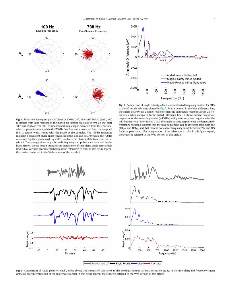
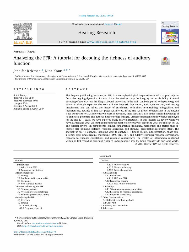
Fig. 4. Unit circle histogram plots of phase of 100 Hz (left, blue) and 700 Hz (right, red)responses from FFRs recorded in the guinea pig inferior colliculus to two ‘a's that start180� out of phase. The 100 Hz fundamental frequency is extracted from the envelope,which is phase invariant, while the 700 Hz first formant is extracted from the temporalfine structure, which varies with the phase of the stimulus. The 100 Hz responsesmaintain a consistent phase angle regardless of the stimulus polarity while the 700 Hzresponses flip their phase angle by ~180� , similar to the phase shift between the two ‘a’stimuli. The average phase angle for each frequency and polarity are indicated by theblack arrows, whose length indicates the consistency of that phase angle across trials(individual vectors). (For interpretation of the references to color in this figure legend,the reader is referred to the Web version of this article.)

Fig. 5. Comparison of single polarity (black), added (blue), and subtracted (red) FFRs to the evoking stimulus, a short, 40-ms ‘da’ (gray) in the time (left) and frequency (right)domains. (For interpretation of the references to color in this figure legend, the reader is referred to the Web version of this article.)

Fig. 6. Comparison of single polarity, added, and subtracted frequency content for FFRsto the 40ms ‘da’ stimulus plotted in Fig. 5. As can be seen in the blue difference line,the single polarity has a larger response than the subtracted response across all fre-quencies, while compared to the added FFR (black line), it shows similar magnituderesponses for the lower frequencies (<400Hz) and greater response magnitude for themid frequencies (~500e800 Hz). That the single polarity response has the largest mid-frequency encoding suggests that the mid frequencies can be extracted from both theFFRENV and FFRTFS and that there is not a clear frequency cutoff between ENV and TFSfor a complex sound. (For interpretation of the references to color in this figure legend,the reader is referred to the Web version of this article.)

J. Krizman, N. Kraus / Hearing Research 382 (2019) 107779 7

Fig. 7. Comparison of added (blue) and subtracted (red) FFRs in response to a stimulusthat consists of noise shaped by the ‘da’ envelope (black, top time domain, bottomfrequency domain). Because the carrier is noise, there are no resolvable frequenciescontained within the stimulus. The only spectral information can be extracted from theenvelope. Therefore, the FFR to this stimulus is only an envelope response, no temporalfine structure is encoded. This demonstrates that the added response is an enveloperesponse that consists of both the fundamental frequency (100Hz in this case) and itslower harmonics, in this case, up to ~500 Hz. When there is no spectral energy in thestimulus, there is no subtracted response. (For interpretation of the references to colorin this figure legend, the reader is referred to the Web version of this article.)

J. Krizman, N. Kraus / Hearing Research 382 (2019) 1077798

(Hornickel et al., 2009; Johnson et al., 2008). An irregular sound likean environmental noise or the baby cry illustrated in Fig. 1 will havedifferent acoustical landmarks that will inform the decision of theresponse peaks of interest. We often see FFR peaks that correspondto transition points in the stimulus (e.g., the onset of voicing) or thecessation of the sound.

Recording and processing parameters can also affect themorphology, timing, or magnitude of peaks in the FFR. Changes in

Fig. 8. FFRs collected from the same participants with (black) and without (red) jitter in thestimulus can have catastrophic effects on the recorded response, serving to low-pass filter tjitter increases, response peaks will be increasingly ablated, with the largest effects being ondomain in the single polarity, added, and subtracted responses (top), which makes peak-pentirely the F0, though the magnitude of F0 encoding is diminished compared to when therfigure legend, the reader is referred to the Web version of this article.)

stimulus intensity often affect the robustness and timing of FFRpeaks differently, with onset peaks being the most robust to in-tensity reductions (Akhoun et al., 2008). Binaural stimuli evokelarger FFRs and, in some cases, earlier peak latencies than stimulipresented monaurally (Parbery-Clark et al., 2013). To elicit a robustresponse to all peaks across the largest number of individuals, wepresent monaural sounds at ~80 dB SPL and binaural sounds at~70e75 dB SPL. Like ABR, rate can also affect FFR peak timing, withfaster stimulus rates resulting in later peak latency, most notablyobserved for the onset peaks (Krizman et al., 2010). As a measure ofperiodicity of the F0, peak picking is only done on single-polarity oradded-polarity responses. Peak timing appears to be consistentacross polarities, which is expected given that they are largelydetermined by the phase-invariant temporal envelope, thoughthere is a tendency for peaks in the added response to be earlier(Kumar et al., 2013).

While we use the same procedure for peak-picking acrossstimuli, we have developed a particular nomenclature for our short,40-ms ‘da’ stimulus. For our other stimuli we use the expected timeto name the peak (e.g., peak 42 occurs ~42ms post stimulus onset;Fig. 9 (White-Schwoch et al., 2015);), or we will number the peakssequentially (e.g., peak 1 is the earliest peak identified in theresponse (Hornickel et al., 2009)). On the other hand, the short ‘da’has peaks named ‘V’, ‘A’, ‘C’, ‘D’, ‘E’, ‘F’, ‘O’ (Fig. 9, King et al., 2002;Russo et al., 2004). As described previously (Krizman et al., 2012a),Peak V is the positive amplitude deflection corresponding to theonset of the stimulus and occurs ~7e8ms after stimulus onset, A isthe negative amplitude deflection that immediately follows V. PeakC reflects the transition from the onset burst to the onset of voicing.Peaks D, E, and F are negative amplitude deflections correspondingto the voicing of the speech sound, and as such are spaced ~8msapart (i.e., the period of the fundamental) occurring at ~22, ~31, and~39ms, respectively. O is the negative amplitude deflection inresponse to the offset of the sound and occurs at about 48ms poststimulus onset (i.e., 8 ms after stimulus cessation). We havecollected FFR to this stimulus in thousands of individuals across thelifespan and have created a published normative dataset (Skoe

timing of the stimulus presentation. Subtle variations in the presentation timing of thehe response with a lower high-frequency cutoff as the jitter increases. Thus, as timingthe highest frequencies. Magnitude of the response is severely diminished in the time

icking difficult. The frequency encoding is also affected. The response becomes almoste is no presentation jitter (bottom). (For interpretation of the references to color in this

Fig. 9. Peak-naming conventions for peaks in the short-da (top) and long-da (bottom) FFRs. Other stimuli that we have used in the lab, such as ga or ba, use a naming conventionsimilar to the long-da.

Fig. 10. Autocorrelation to extract the F0 of a rising ‘ya’ syllable. On the left is the pitch extraction over time (yellow squares) relative to the pitch of the stimulus (black dots). On theright is the autocorrelelogram of the FFR. The timing shift (i.e., lag, in ms) to achieve the maximum correlation (i.e., the darker red) corresponds to the periodicity of the fundamentalfrequency. As this periodicity is contained within the temporal envelope of the FFR, it is only evident on single polarity (left) or added (middle) responses. No F0 periodicity isevident in the subtracted (right) response. (For interpretation of the references to color in this figure legend, the reader is referred to the Web version of this article.)

J. Krizman, N. Kraus / Hearing Research 382 (2019) 107779 9

et al., 2015) that we refer to when picking peaks.Several measures are available to analyze peaks. A primary

measure is the absolute latency of a single peak, such as an onsetpeak. When looking at response peaks reflecting the periodicity of asound, we will generally average these peaks over a specific regionof the response, such as the formant transition. We will alsocompare relative timing across FFRs to different stimuli or to thesame sound under different recording conditions, such as a ‘da’presented in quiet or in the presence of background noise. Becausenoise delays the timing of peaks in the FFR, we can look at the sizeof these degradative effects by calculating latency shifts for specificFFR peaks (Parbery-Clark et al., 2009). Alternatively, we cancalculate a global measure of timing shift by performing a stimulus-response correlation (see below), which provides a measure of thetiming shift necessary to achieve the maximum absolute-valuecorrelation between the stimulus and the response. We can simi-larly do this with two different FFRs (see response-response cor-relation below). These methods provide a measure of global timingin the subtracted FFR, while peak-picking can only be performed onadded or single-polarity FFRs since the prominent peaks are re-sponses to the temporal envelope.

4.2.2. Frequency-specific timing4.2.2.1. Autocorrelation. Autocorrelation can be used to measure

periodicity of a signal and so can be used to gauge pitch tracking inan FFR (e.g., see Carcagno and Plack, 2011; Wong et al., 2007). It is astandard procedure that time-shifts a waveform (W) with respectto a copy of itself (W0) and correlates W to W0 at many such timeshifts. As a measure of F0 periodicity, it is meaningful on singlepolarity or added polarity FFRs (Fig. 10). The goal is to identify thelag (L) at which the maximum correlation occurs (i.e., Lmax),excluding a time shift of zero. The maximum correlation is referredto as rmax. The maximum lag occurs at the period of the funda-mental frequency (i.e., F0¼1/Lmax Hz. Thus, for an FFR response to aspeech syllable with a 100Hz F0 we would expect a maximumautocorrelation between W and W’ at a lag of ~0.01 s, or 10ms.

If the stimulus has an F0 that changes over time or if there is adesire to examine changes over the duration of a response to a non-changing F0, you can use a sliding window to analyze the max lagand correlation at discrete points along the response. For example,for a 230ms stimulus with an F0 that rises linearly from 130 Hz to220 Hz, as in Fig. 10, if we look at a specific time point for thatstimulus, there will be a specific F0 value at that point, such as130 Hz at t¼ 0ms, 175 Hz at t¼ 115ms, and 220 Hz at t¼ 230ms.The instantaneous frequency at any given point can be derived byrunning an autocorrelation over small, overlapping segments of thewaveform. Typically, we use a 40ms window, with a 39ms overlap,starting with awindow centered over t¼ 0ms. An rmax and Lmax are

J. Krizman, N. Kraus / Hearing Research 382 (2019) 10777910

assigned to the center time point of each window to provide ameasure of pitch tracking over time (Fig.10). As this measure can berun on both the stimulus and the response, we can use the outputto determine the pitch-tracking accuracy of the brain response bycomputing the difference in extracted F0 between the stimulus andFFR at each time point. Because the response will always lag thestimulus by a fixed amount (about 8ms), it is necessary to makethat adjustment. So, the pitch of the stimulus at time¼ 50mswould be compared to the pitch in the response at time¼ 58ms.We then sum the absolute values of the frequency differences ateach point to calculate a “frequency error”, where 0 indicates per-fect pitch tracking and larger numbers indicate poorer pitch-tracking (i.e., greater differences between stimulus and response).A sliding-window fast-Fourier transform (FFT) approach (describedbelow) can also be used to determine pitch-tracking accuracy (e.g.,see Maggu et al., 2018; Song et al., 2008).

4.2.2.2. Phase consistency. Peak-picking on the time domainwaveform requires averaging responses to a large number ofstimulus presentations to generate a robust FFR with peaks suffi-ciently above the noise floor, operationally defined as peaks in theresponse that are larger in amplitude than the non-stimulusresponse activity. Moreover, while these peaks occur at the peri-odicity of lower frequency components of the stimulus, they areinfluenced by all frequencies in the stimulus and thus reflectbroadband timing of the FFR. An alternative approach to looking atFFR timing is to analyze the phase of individual frequencies over thecourse of the response to determine how consistent the phase for agiven frequency is across individual trials (i.e., responses to indi-vidual stimulus presentations). In addition to providing frequency-specific timing information, this technique has the added benefit ofextracting meaningful information with fewer numbers of sweepsand is less susceptible to artifacts (Zhu et al., 2013), though we stillencourage artifact rejection prior to processing to remove largerartifact. Furthermore, though it must be performed on data that hasmaintained single-trial responses, it can be performed on singlepolarity, added polarity, and subtracted polarity responses and canbe examined by averaging over the whole FFR or by using a sliding-windowapproach. This measure hasmany names, including phase-

Fig. 11. Phase consistency of a ‘dipping da’ and a ‘level-F0 da’ using single polarity, added pothe fundamental frequency, second harmonic and formant frequencies all show the strongfrequencies, below ~600 Hz, and subtracting emphasizes the phase coherence of the higherlegend, the reader is referred to the Web version of this article.)

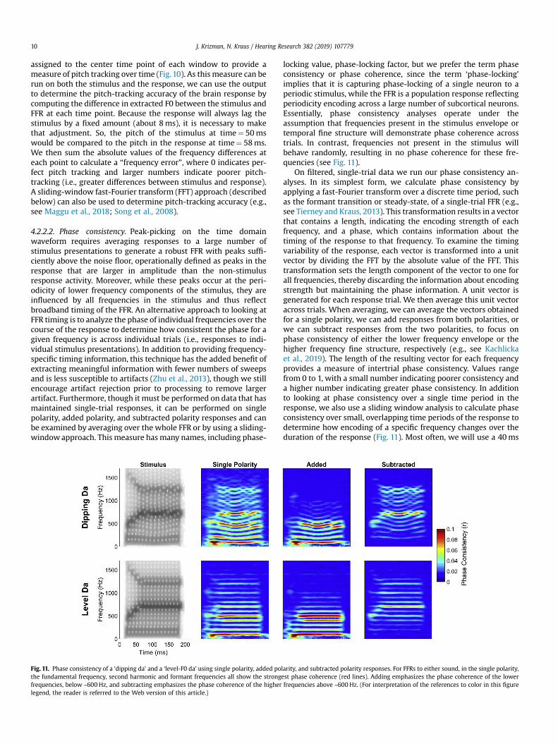
locking value, phase-locking factor, but we prefer the term phaseconsistency or phase coherence, since the term ‘phase-locking’implies that it is capturing phase-locking of a single neuron to aperiodic stimulus, while the FFR is a population response reflectingperiodicity encoding across a large number of subcortical neurons.Essentially, phase consistency analyses operate under theassumption that frequencies present in the stimulus envelope ortemporal fine structure will demonstrate phase coherence acrosstrials. In contrast, frequencies not present in the stimulus willbehave randomly, resulting in no phase coherence for these fre-quencies (see Fig. 11).

On filtered, single-trial data we run our phase consistency an-alyses. In its simplest form, we calculate phase consistency byapplying a fast-Fourier transform over a discrete time period, suchas the formant transition or steady-state, of a single-trial FFR (e.g.,see Tierney and Kraus, 2013). This transformation results in a vectorthat contains a length, indicating the encoding strength of eachfrequency, and a phase, which contains information about thetiming of the response to that frequency. To examine the timingvariability of the response, each vector is transformed into a unitvector by dividing the FFT by the absolute value of the FFT. Thistransformation sets the length component of the vector to one forall frequencies, thereby discarding the information about encodingstrength but maintaining the phase information. A unit vector isgenerated for each response trial. We then average this unit vectoracross trials. When averaging, we can average the vectors obtainedfor a single polarity, we can add responses from both polarities, orwe can subtract responses from the two polarities, to focus onphase consistency of either the lower frequency envelope or thehigher frequency fine structure, respectively (e.g., see Kachlickaet al., 2019). The length of the resulting vector for each frequencyprovides a measure of intertrial phase consistency. Values rangefrom 0 to 1, with a small number indicating poorer consistency anda higher number indicating greater phase consistency. In additionto looking at phase consistency over a single time period in theresponse, we also use a sliding window analysis to calculate phaseconsistency over small, overlapping time periods of the response todetermine how encoding of a specific frequency changes over theduration of the response (Fig. 11). Most often, we will use a 40ms

larity, and subtracted polarity responses. For FFRs to either sound, in the single polarity,est phase coherence (red lines). Adding emphasizes the phase coherence of the lowerfrequencies above ~600 Hz. (For interpretation of the references to color in this figure

J. Krizman, N. Kraus / Hearing Research 382 (2019) 107779 11

Hanning-ramped window with a 39ms overlap, which results inphase consistency being calculated from 0 to 40ms, 1e41ms,2e42ms, etc. (e.g., see Bonacina et al., 2018; White-Schwoch et al.,2016a). The phase consistency of a single frequency of interest, forexample, a 100Hz F0, or an average of frequencies centered arounda frequency of interest (e.g., 100 Hz± 10Hz) is then analyzed.Instead of using an FFT to examine phase consistency, other signalprocessing approaches to determine the instantaneous phase of theresponse at specific frequencies, such as wavelets, can also be used(e.g., see Roque et al., 2019).

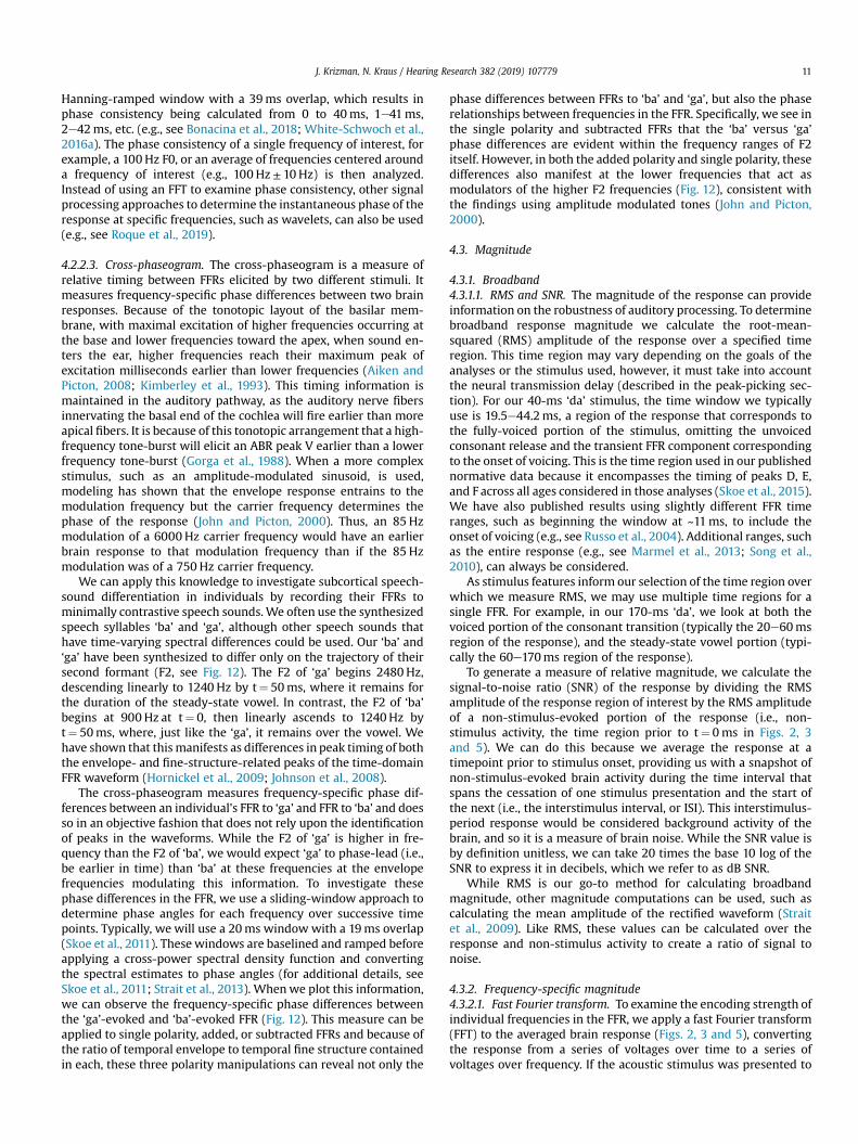
4.2.2.3. Cross-phaseogram. The cross-phaseogram is a measure ofrelative timing between FFRs elicited by two different stimuli. Itmeasures frequency-specific phase differences between two brainresponses. Because of the tonotopic layout of the basilar mem-brane, with maximal excitation of higher frequencies occurring atthe base and lower frequencies toward the apex, when sound en-ters the ear, higher frequencies reach their maximum peak ofexcitation milliseconds earlier than lower frequencies (Aiken andPicton, 2008; Kimberley et al., 1993). This timing information ismaintained in the auditory pathway, as the auditory nerve fibersinnervating the basal end of the cochlea will fire earlier than moreapical fibers. It is because of this tonotopic arrangement that a high-frequency tone-burst will elicit an ABR peak V earlier than a lowerfrequency tone-burst (Gorga et al., 1988). When a more complexstimulus, such as an amplitude-modulated sinusoid, is used,modeling has shown that the envelope response entrains to themodulation frequency but the carrier frequency determines thephase of the response (John and Picton, 2000). Thus, an 85 Hzmodulation of a 6000 Hz carrier frequency would have an earlierbrain response to that modulation frequency than if the 85 Hzmodulation was of a 750 Hz carrier frequency.

We can apply this knowledge to investigate subcortical speech-sound differentiation in individuals by recording their FFRs tominimally contrastive speech sounds.We often use the synthesizedspeech syllables ‘ba’ and ‘ga’, although other speech sounds thathave time-varying spectral differences could be used. Our ‘ba’ and‘ga’ have been synthesized to differ only on the trajectory of theirsecond formant (F2, see Fig. 12). The F2 of ‘ga’ begins 2480Hz,descending linearly to 1240 Hz by t¼ 50ms, where it remains forthe duration of the steady-state vowel. In contrast, the F2 of ‘ba’begins at 900 Hz at t¼ 0, then linearly ascends to 1240Hz byt¼ 50ms, where, just like the ‘ga’, it remains over the vowel. Wehave shown that thismanifests as differences in peak timing of boththe envelope- and fine-structure-related peaks of the time-domainFFR waveform (Hornickel et al., 2009; Johnson et al., 2008).

The cross-phaseogram measures frequency-specific phase dif-ferences between an individual's FFR to ‘ga’ and FFR to ‘ba’ and doesso in an objective fashion that does not rely upon the identificationof peaks in the waveforms. While the F2 of ‘ga’ is higher in fre-quency than the F2 of ‘ba’, we would expect ‘ga’ to phase-lead (i.e.,be earlier in time) than ‘ba’ at these frequencies at the envelopefrequencies modulating this information. To investigate thesephase differences in the FFR, we use a sliding-window approach todetermine phase angles for each frequency over successive timepoints. Typically, we will use a 20ms window with a 19ms overlap(Skoe et al., 2011). These windows are baselined and ramped beforeapplying a cross-power spectral density function and convertingthe spectral estimates to phase angles (for additional details, seeSkoe et al., 2011; Strait et al., 2013). Whenwe plot this information,we can observe the frequency-specific phase differences betweenthe ‘ga’-evoked and ‘ba’-evoked FFR (Fig. 12). This measure can beapplied to single polarity, added, or subtracted FFRs and because ofthe ratio of temporal envelope to temporal fine structure containedin each, these three polarity manipulations can reveal not only the

phase differences between FFRs to ‘ba’ and ‘ga’, but also the phaserelationships between frequencies in the FFR. Specifically, we see inthe single polarity and subtracted FFRs that the ‘ba’ versus ‘ga’phase differences are evident within the frequency ranges of F2itself. However, in both the added polarity and single polarity, thesedifferences also manifest at the lower frequencies that act asmodulators of the higher F2 frequencies (Fig. 12), consistent withthe findings using amplitude modulated tones (John and Picton,2000).

4.3. Magnitude

4.3.1. Broadband4.3.1.1. RMS and SNR. The magnitude of the response can provideinformation on the robustness of auditory processing. To determinebroadband response magnitude we calculate the root-mean-squared (RMS) amplitude of the response over a specified timeregion. This time region may vary depending on the goals of theanalyses or the stimulus used, however, it must take into accountthe neural transmission delay (described in the peak-picking sec-tion). For our 40-ms ‘da’ stimulus, the time window we typicallyuse is 19.5e44.2ms, a region of the response that corresponds tothe fully-voiced portion of the stimulus, omitting the unvoicedconsonant release and the transient FFR component correspondingto the onset of voicing. This is the time region used in our publishednormative data because it encompasses the timing of peaks D, E,and F across all ages considered in those analyses (Skoe et al., 2015).We have also published results using slightly different FFR timeranges, such as beginning the window at ~11ms, to include theonset of voicing (e.g., see Russo et al., 2004). Additional ranges, suchas the entire response (e.g., see Marmel et al., 2013; Song et al.,2010), can always be considered.

As stimulus features inform our selection of the time region overwhich we measure RMS, we may use multiple time regions for asingle FFR. For example, in our 170-ms ‘da’, we look at both thevoiced portion of the consonant transition (typically the 20e60msregion of the response), and the steady-state vowel portion (typi-cally the 60e170ms region of the response).

To generate a measure of relative magnitude, we calculate thesignal-to-noise ratio (SNR) of the response by dividing the RMSamplitude of the response region of interest by the RMS amplitudeof a non-stimulus-evoked portion of the response (i.e., non-stimulus activity, the time region prior to t¼ 0ms in Figs. 2, 3and 5). We can do this because we average the response at atimepoint prior to stimulus onset, providing us with a snapshot ofnon-stimulus-evoked brain activity during the time interval thatspans the cessation of one stimulus presentation and the start ofthe next (i.e., the interstimulus interval, or ISI). This interstimulus-period response would be considered background activity of thebrain, and so it is a measure of brain noise. While the SNR value isby definition unitless, we can take 20 times the base 10 log of theSNR to express it in decibels, which we refer to as dB SNR.

While RMS is our go-to method for calculating broadbandmagnitude, other magnitude computations can be used, such ascalculating the mean amplitude of the rectified waveform (Straitet al., 2009). Like RMS, these values can be calculated over theresponse and non-stimulus activity to create a ratio of signal tonoise.

4.3.2. Frequency-specific magnitude4.3.2.1. Fast Fourier transform. To examine the encoding strength ofindividual frequencies in the FFR, we apply a fast Fourier transform(FFT) to the averaged brain response (Figs. 2, 3 and 5), convertingthe response from a series of voltages over time to a series ofvoltages over frequency. If the acoustic stimulus was presented to

Fig. 12. Comparison of single polarity, added, and subtracted phaseograms comparing ba versus ga. Based on the frequency contents of ba and ga, it is expected that ga shouldphase-lead ba during the formant transition because it is higher in frequency, and thus activates more basal regions of the basal membrane than ba. We have typically reported itusing ‘added’ polarity responses, which show a phase differences at a lower frequency than would be expected based on where in frequency these stimuli differ. Interestingly,however, if we compare the single polarity ba versus ga, which contain both the temporal envelope and fine structure, we see the greatest differences in the F2 frequencies (i.e.,where they differ), however, there is also a ga phase lead in the lower frequency, suggesting that the second formant frequencies are encoded at that lower modulation rate. Themodulation frequency differences become emphasized when we add polarities while the differences at the F2 frequencies become emphasized in the subtracted response. Asexpected, there are no phase or timing differences in the steady state ‘a’, which is where the two stimuli have equivalent spectral features. Phase differences (in radians) areindicated by color, with warmer colors indicating that ga phase leads ba. Green indicates no phase differences, and cooler colors would indicate ba phase leading ga. (For inter-pretation of the references to color in this figure legend, the reader is referred to the Web version of this article.)

J. Krizman, N. Kraus / Hearing Research 382 (2019) 10777912

the participant in alternating polarities, then when creating anaverage of the response, it is possible to look at frequency-specificmagnitude in the single polarity, the added polarity (which en-hances temporal envelope frequencies, including the F0 and lowerharmonics), and the subtracted polarity (which accentuates theresponse to the temporal fine structure, or middle and high har-monics) (Figs. 3 and 5).

Our approach to generating the spectrum of a selected FFR timerange involves if necessary, zero padding to increase the spectralresolution to at least 1 Hz, then, applying a Hanning window (otherwindowing approaches may be used) and a ramp equal to one halfthe time range over which the FFT was calculated (i.e., ramp up tothe midway point of the selected time range and then ramp downto the end of the time range), though shorter ramps can be used.Any time region can be used to calculate the FFT, but like RMScalculations, the window needs to account for the neural trans-mission delay, and it should not extend beyond the response re-gion. It should also contain, at minimum, one cycle of the periodcorresponding to the frequency of interest. For example, our long‘da’ has an F0 of 100Hz, the period of which is 10ms, meaning theresponse window over which F0 encoding strength can bemeasured must be at least 10ms in duration, but it is good practiceto at least double this minimum time length.

There are a few approaches to extract the amplitude from thespectrum. When looking at F0 encoding, we may extract theamplitude at a single frequency, such as 100Hz from the exampleabove, or we may average over a range of frequencies (e.g., seeKrizman et al., 2012a), especially if the F0 changes overtime, as inthe case of our short ‘da’, whose F0 ramps from 103 to 125 Hz overthe utterance. We may use an even broader range to capture the

variation in frequency encoding near the F0 that is observed acrossindividual responses (e.g., see Kraus et al., 2016a; Kraus et al.,2016b; Skoe et al., 2015). A similar method is used to investigatehigher frequency encoding, where we measure harmonic encodingat individual harmonic frequencies (e.g., see Anderson et al.,2013b), or average across a range of frequencies centered at thefrequency of interest (e.g., see White-Schwoch et al., 2015).Because, by definition, during the formant transition formantsmove across frequencies (e.g., the first formant of the 40-ms ‘da’changes from 220 to 720 Hz), we average the amplitude acrossthese frequencies to provide a snapshot of formant encoding (e.g.,see Krizman et al., 2012a). We also average the amplitude of indi-vidual harmonics over a steady-state vowel to get a general mea-sure of FFR harmonic strength (e.g., see Parbery-Clark et al., 2009).

Beyond examining a single time window, we can use a slidingwindow approach to explore changes in frequency encoding overthe duration of the response. This short-term Fourier transformtechnique is especially informative for stimuli that have a changingF0 or if you want to examine a response to a formant transition.Similar to other sliding window procedures described above, wetypically use a 40ms window, centered beginning at t¼ 0ms andmoving over the duration of the response with a 39ms overlapacross successive windows, providing 1ms temporal resolution tofrequency encoding. We plot these time-varying spectral powers asspectrograms (see Fig. 13).

4.4. Fidelity

Response fidelity is assessed by comparing FFR consistencywithin or across sessions, either to itself, another FFR, or the

Fig. 13. Spectrograms of the stimuli and single polarity, added, and subtracted FFRs for ‘ba’ (top) and ‘ga’ (bottom). The rising F2 of ‘ba’ and the falling F2 of ‘ga’ are maintained in thesingle polarity and subtracted responses while the added response highlights how these formant differences are reflected in the lower frequencies. These frequency differences canalso be seen in the cross-phaseogram (Fig. 12).

J. Krizman, N. Kraus / Hearing Research 382 (2019) 107779 13

stimulus. Phase consistency may also be considered a frequency-specific measure of fidelity, but because it is also a timing-dependent measure, phase consistency has been discussed in thetiming section. Additionally, while we typically perform thefollowing measures in the time domain, any of these can be per-formed after transforming the time domain waveform into thefrequency domain via a fast-Fourier transform (FFT).

4.4.1. Stimulus-to-response correlationAs the name implies, stimulus-to-response correlation assesses

the morphological similarity of the response with its evokingstimulus. We first must filter the stimulus to match the response,generally, from 70 to 2000Hz using a second-order Butterworthfilter, but these parameters vary depending on the frequency con-tent of the FFR being analyzed. For example, a lower cutoff value forthe low-pass filter may be preferable for analyzing an addedresponse, while a higher frequency may be used when analyzing asubtracted response. We do this to generate a stimulus waveformthat will more highly correlate with the FFR, enabling better com-parison of fidelity differences across participants.

We then run a standard cross-correlation between the filteredstimulus and response over a time region of interest (e.g.,19.5e44.2ms for FFR to short ‘da’), which may vary depending onthe acoustic features of interest, the stimulus used to evoke the FFR,or the research question. This procedure is similar to that describedin the autocorrelation section, except the FFR waveform (W) iscorrelated with the stimulus (S) and not a copy of itself. W iscorrelated with S, across a series of time shifts for one of the twowaveforms, such that at time-shift t¼ 0, the original, unshiftedwaveforms W and S are correlated. At t¼ 1, W has been shifted byone, while S remains unshifted and the cross-correlation for thatlag is calculated, providing us with a Pearson product-momentcorrelation (though other correlation methods can be used). Intheory, W can also be shifted by negative values in a similarmanner, but because the brain response cannot temporally lead thestimulus, we do not perform stimulus-to-response calculations inthis direction. The maximum absolute-value correlation (r) at a lag(t) that accounts for neural transmission delay, typically a 7e10mslag window, is obtained. Because the correlation values range fromr¼�1 (identical but 180� out of phase) to 0 (no correlation) to 1(identical and in phase), it is possible for the maximum correlation

to be negative. Once the maximum correlation is obtained, it isFisher-transformed to z scores prior to statistical analyses. Thisnatural-log-based transformation normalizes the r distribution sothat the variance of r values across the range �1 to 0 to 1 areequivalently constant. The lag can provide an objective measure ofbroadband timing and so it too is analyzed (e.g., see Tierney et al.,2013).

4.4.2. Response-response correlationTwo FFRs can be correlated with one another. We often collect

FFRs to the same stimulus under different listening conditions, forexample, in quiet and background noise, and then cross-correlatethe two responses (e.g., see Anderson et al., 2013a; Parbery-Clarket al., 2009). The method itself is identical to the cross-correlationmethod used for stimulus-to-response correlations describedabove. Here, an FFR to a stimulus in quiet (WQ) is correlated to anFFR to that same stimulus in background noise (WN) across a seriesof time shifts for WN. For response-response correlations, however,it is appropriate to shift one of the FFRs both forward and backwardin time when cross-correlating the waveforms. In this instance, anegative lag would indicate that the shifted waveform is earlier intime than the comparison FFR, while the opposite would be true fora positive lag. Again, r values are converted to z scores prior tostatistical analyses.

4.4.3. Response consistencyWe can also analyze the within-session correlation of FFR trials,

an analysis that we refer to as response consistency or responsestability. This supplies an index of how stable the FFR is from trial-to-trial. Response consistency calculations capitalize on the largenumber of trials presented to a participant during a session togenerate an averaged FFR. To calculate response consistency, wecorrelate subsets of trials collected during a recording session,generating an r-value that is converted to a z-score prior toanalyzing. The straight (i.e., lag¼ 0) calculation is performed over atime region relevant to the evoking stimulus and/or the questionyou are asking. The closer the r value is to 1, the more consistent thetwo FFR subaverages.

We have used several methods to examine response consis-tency. One method is to average the odd sweeps separate from theeven sweeps (e.g., see Hornickel and Kraus, 2013). This approach

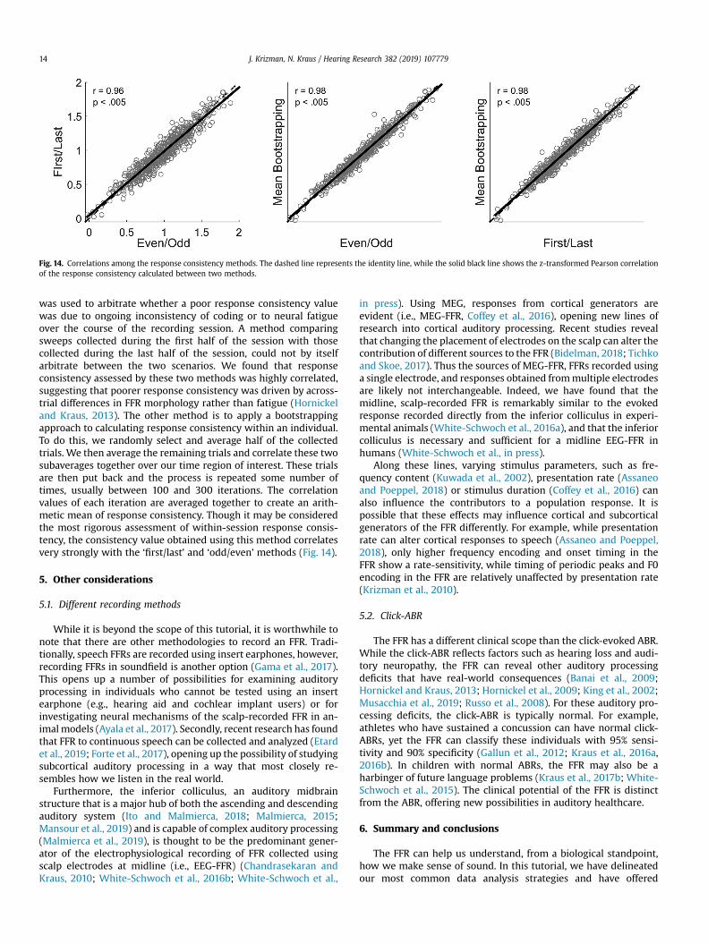
Fig. 14. Correlations among the response consistency methods. The dashed line represents the identity line, while the solid black line shows the z-transformed Pearson correlationof the response consistency calculated between two methods.

J. Krizman, N. Kraus / Hearing Research 382 (2019) 10777914

was used to arbitrate whether a poor response consistency valuewas due to ongoing inconsistency of coding or to neural fatigueover the course of the recording session. A method comparingsweeps collected during the first half of the session with thosecollected during the last half of the session, could not by itselfarbitrate between the two scenarios. We found that responseconsistency assessed by these two methods was highly correlated,suggesting that poorer response consistency was driven by across-trial differences in FFR morphology rather than fatigue (Hornickeland Kraus, 2013). The other method is to apply a bootstrappingapproach to calculating response consistency within an individual.To do this, we randomly select and average half of the collectedtrials. We then average the remaining trials and correlate these twosubaverages together over our time region of interest. These trialsare then put back and the process is repeated some number oftimes, usually between 100 and 300 iterations. The correlationvalues of each iteration are averaged together to create an arith-metic mean of response consistency. Though it may be consideredthe most rigorous assessment of within-session response consis-tency, the consistency value obtained using this method correlatesvery strongly with the ‘first/last’ and ‘odd/even’ methods (Fig. 14).

5. Other considerations

5.1. Different recording methods

While it is beyond the scope of this tutorial, it is worthwhile tonote that there are other methodologies to record an FFR. Tradi-tionally, speech FFRs are recorded using insert earphones, however,recording FFRs in soundfield is another option (Gama et al., 2017).This opens up a number of possibilities for examining auditoryprocessing in individuals who cannot be tested using an insertearphone (e.g., hearing aid and cochlear implant users) or forinvestigating neural mechanisms of the scalp-recorded FFR in an-imalmodels (Ayala et al., 2017). Secondly, recent research has foundthat FFR to continuous speech can be collected and analyzed (Etardet al., 2019; Forte et al., 2017), opening up the possibility of studyingsubcortical auditory processing in a way that most closely re-sembles how we listen in the real world.

Furthermore, the inferior colliculus, an auditory midbrainstructure that is a major hub of both the ascending and descendingauditory system (Ito and Malmierca, 2018; Malmierca, 2015;Mansour et al., 2019) and is capable of complex auditory processing(Malmierca et al., 2019), is thought to be the predominant gener-ator of the electrophysiological recording of FFR collected usingscalp electrodes at midline (i.e., EEG-FFR) (Chandrasekaran andKraus, 2010; White-Schwoch et al., 2016b; White-Schwoch et al.,

in press). Using MEG, responses from cortical generators areevident (i.e., MEG-FFR, Coffey et al., 2016), opening new lines ofresearch into cortical auditory processing. Recent studies revealthat changing the placement of electrodes on the scalp can alter thecontribution of different sources to the FFR (Bidelman, 2018; Tichkoand Skoe, 2017). Thus the sources of MEG-FFR, FFRs recorded usinga single electrode, and responses obtained frommultiple electrodesare likely not interchangeable. Indeed, we have found that themidline, scalp-recorded FFR is remarkably similar to the evokedresponse recorded directly from the inferior colliculus in experi-mental animals (White-Schwoch et al., 2016a), and that the inferiorcolliculus is necessary and sufficient for a midline EEG-FFR inhumans (White-Schwoch et al., in press).

Along these lines, varying stimulus parameters, such as fre-quency content (Kuwada et al., 2002), presentation rate (Assaneoand Poeppel, 2018) or stimulus duration (Coffey et al., 2016) canalso influence the contributors to a population response. It ispossible that these effects may influence cortical and subcorticalgenerators of the FFR differently. For example, while presentationrate can alter cortical responses to speech (Assaneo and Poeppel,2018), only higher frequency encoding and onset timing in theFFR show a rate-sensitivity, while timing of periodic peaks and F0encoding in the FFR are relatively unaffected by presentation rate(Krizman et al., 2010).

5.2. Click-ABR

The FFR has a different clinical scope than the click-evoked ABR.While the click-ABR reflects factors such as hearing loss and audi-tory neuropathy, the FFR can reveal other auditory processingdeficits that have real-world consequences (Banai et al., 2009;Hornickel and Kraus, 2013; Hornickel et al., 2009; King et al., 2002;Musacchia et al., 2019; Russo et al., 2008). For these auditory pro-cessing deficits, the click-ABR is typically normal. For example,athletes who have sustained a concussion can have normal click-ABRs, yet the FFR can classify these individuals with 95% sensi-tivity and 90% specificity (Gallun et al., 2012; Kraus et al., 2016a,2016b). In children with normal ABRs, the FFR may also be aharbinger of future language problems (Kraus et al., 2017b; White-Schwoch et al., 2015). The clinical potential of the FFR is distinctfrom the ABR, offering new possibilities in auditory healthcare.

6. Summary and conclusions

The FFR can help us understand, from a biological standpoint,how we make sense of sound. In this tutorial, we have delineatedour most common data analysis strategies and have offered

J. Krizman, N. Kraus / Hearing Research 382 (2019) 107779 15

guidelines for aligning these analyses with specific applications. Itis our hope that this tutorial will fuel the apparent global surge ofinterest in using the FFR in clinics and research laboratories. For thefuture, we are excited to learn how the FFR can help us get closer todiscovering how our brains go about the formidable business ofreconstructing our sonic world.

Acknowledgements

The authors thank everyone in the Auditory Neuroscience Lab-oratory, past and present, for their help with data collection andprocessing. The authors also thank Trent Nicol and Travis White-Schwoch for their comments on an earlier version of the manu-script. This workwas supported by the National Science Foundation(BCS-1430400), National Institutes of Health (R01 HD069414), theNational Association of MusicMerchants, the Dana Foundation, andthe Knowles Hearing Center, Northwestern University. The authorsdeclare no conflicts of interest.

Appendix A. Supplementary data

Supplementary data to this article can be found online athttps://doi.org/10.1016/j.heares.2019.107779.

References

Aiken, S.J., Picton, T.W., 2008. Envelope and spectral frequency-following responsesto vowel sounds. Hear. Res. 245, 35e47.

Akhoun, I., Gallego, S., Moulin, A., Menard, M., Veuillet, E., Berger-Vachon, C.,Collet, L., Thai-Van, H., 2008. The temporal relationship between speech audi-tory brainstem responses and the acoustic pattern of the phoneme/ba/innormal-hearing adults. Clin. Neurophysiol. 119, 922e933.

Anderson, S., Skoe, E., Chandrasekaran, B., Kraus, N., 2010a. Neural timing is linkedto speech perception in noise. J. Neurosci. 30, 4922e4926.

Anderson, S., White-Schwoch, T., Parbery-Clark, A., Kraus, N., 2013a. Reversal of age-related neural timing delays with training. Proc. Natl. Acad. Sci. 110, 4357e4362.

Anderson, S., Skoe, E., Chandrasekaran, B., Zecker, S., Kraus, N., 2010b. Brainstemcorrelates of speech-in-noise perception in children. Hear. Res. 270, 151e157.

Anderson, S., Parbery-Clark, A., White-Schwoch, T., Drehobl, S., Kraus, N., 2013b.Effects of hearing loss on the subcortical representation of speech cues.J. Acoust. Soc. Am. 133, 3030e3038.

Assaneo, M.F., Poeppel, D., 2018. The coupling between auditory and motor corticesis rate-restricted: evidence for an intrinsic speech-motor rhythm. Sci. Adv. 4,eaao3842.

Ayala, Y.A., Lehmann, A., Merchant, H., 2017. Monkeys share the neurophysiologicalbasis for encoding sound periodicities captured by the frequency-followingresponse with humans. Sci. Rep. 7, 16687.

Banai, K., Hornickel, J., Skoe, E., Nicol, T., Zecker, S., Kraus, N., 2009. Reading andsubcortical auditory function. Cerebr. Cortex 19, 2699e2707.

Bidelman, G.M., 2015. Multichannel recordings of the human brainstem frequency-following response: scalp topography, source generators, and distinctions fromthe transient ABR. Hear. Res. 323, 68e80.

Bidelman, G.M., 2018. Subcortical sources dominate the neuroelectric auditoryfrequency-following response to speech. Neuroimage 175, 56e69.

BinKhamis, G., L�eger, A., Bell, S.L., Prendergast, G., O'Driscoll, M., Kluk, K., 2019.Speech auditory brainstem responses: effects of background, stimulus duration,consonantevowel, and number of epochs. Ear Hear. 40, 659e670.

Bonacina, S., Krizman, J., White-Schwoch, T., Kraus, N., 2018. Clapping in timeparallels literacy and calls upon overlapping neural mechanisms in earlyreaders. Ann. N. Y. Acad. Sci. 1423, 338e348.

Carcagno, S., Plack, C.J., 2011. Subcortical plasticity following perceptual learning ina pitch discrimination task. J. Assoc. Res. Otolaryngol. 12, 89e100.

Chandrasekaran, B., Kraus, N., 2010. The scalp-recorded brainstem response tospeech: neural origins and plasticity. Psychophysiology 47, 236e246.

Chen, J., Liang, C., Wei, Z., Cui, Z., Kong, X., Dong, C.j., Lai, Y., Peng, Z., Wan, G., 2019.Atypical longitudinal development of speech-evoked auditory brainstemresponse in preschool children with autism spectrum disorders. Autism Res. 12(7), 1022e1031.

Coffey, E.B., Herholz, S.C., Chepesiuk, A.M., Baillet, S., Zatorre, R.J., 2016. Corticalcontributions to the auditory frequency-following response revealed by MEG.Nat. Commun. 7.

Etard, O., Kegler, M., Braiman, C., Forte, A.E., Reichenbach, T., 2019. Decoding ofselective attention to continuous speech from the human auditory brainstemresponse. Neuroimage 200, 1e11.

Forte, A.E., Etard, O., Reichenbach, T., 2017. The human auditory brainstem responseto running speech reveals a subcortical mechanism for selective attention. elife6, e27203.

Galbraith, G.C., Jhaveri, S.P., Kuo, J., 1997. Speech-evoked brainstem frequency-following responses during verbal transformations due to word repetition.Electroencephalogr. Clin. Neurophysiol. 102, 46e53.

Galbraith, G.C., Arbagey, P.W., Branski, R., Comerci, N., Rector, P.M., 1995. Intelligiblespeech encoded in the human brain stem frequency-following response. Neu-roreport 6, 2363e2367.

Galbraith, G.C., Bhuta, S.M., Choate, A.K., Kitahara, J.M., Mullen Jr., T.A., 1998. Brainstem frequency-following response to dichotic vowels during attention. Neu-roreport 9, 1889e1893.

Gallun, F., Diedesch, A.C., Kubli, L.R., Walden, T.C., Folmer, R., Lewis, M.S.,McDermott, D.J., Fausti, S.A., Leek, M.R., 2012. Performance on tests of centralauditory processing by individuals exposed to high-intensity blasts. J. Rehabil.Res. Dev. 49, 1005.

Gama, N., Peretz, I., Lehmann, A., 2017. Recording the human brainstem frequency-following-response in the free-field. J. Neurosci. Methods 280, 47e53.

Gorga, M.P., Kaminski, J.R., Beauchaine, K.A., Jesteadt, W., 1988. Auditory brainstemresponses to tone bursts in normally hearing subjects. J. Speech Lang. Hear. Res.31, 87e97.

Greenberg, S., Poeppel, D., Roberts, T., 1998. A space-time theory of pitch and timbrebased on cortical expansion of the cochlear traveling wave delay. In: Proc. 11thInt. Symp. On Hearing, pp. 257e262.

Greenwood, D.D., 1961. Critical bandwidth and the frequency coordinates of thebasilar membrane. J. Acoust. Soc. Am. 33, 1344e1356.

Hornickel, J., Kraus, N., 2013. Unstable representation of sound: a biological markerof dyslexia. J. Neurosci. 33, 3500e3504.

Hornickel, J., Knowles, E., Kraus, N., 2012. Test-retest consistency of speech-evokedauditory brainstem responses in typically-developing children. Hear. Res. 284,52e58.

Hornickel, J., Skoe, E., Nicol, T., Zecker, S., Kraus, N., 2009. Subcortical differentiationof voiced stop consonants: relationships to reading and speech in noiseperception. Proc. Natl. Acad. Sci. U.S.A. 106, 13022e13027.

Ito, T., Malmierca, M.S., 2018. Neurons, connections, and microcircuits of the inferiorcolliculus. In: The Mammalian Auditory Pathways. Springer, pp. 127e167.

Jeng, F.-C., Hu, J., Dickman, B., Montgomery-Reagan, K., Tong, M., Wu, G., Lin, C.-D.,2011. Cross-linguistic comparison of frequency-following responses to voicepitch in American and Chinese neonates and adults. Ear Hear. 32, 699e707.

John, M., Picton, T., 2000. Human auditory steady-state responses to amplitude-modulated tones: phase and latency measurements. Hear. Res. 141, 57e79.

Johnson, K.L., Nicol, T., Zecker, S.G., Bradlow, A.R., Skoe, E., Kraus, N., 2008. Brain-stem encoding of voiced consonant-vowel stop syllables. Clin. Neurophysiol.119, 13p.

Kachlicka, M., Saito, K., Tierney, A., 2019. Successful second language learning is tiedto robust domain-general auditory processing and stable neural representationof sound. Brain Lang. 192, 15e24.

Kimberley, B.P., Brown, D.K., Eggermont, J.J., 1993. Measuring human cochleartraveling wave delay using distortion product emission phase responses.J. Acoust. Soc. Am. 94, 1343e1350.

King, C., Warrier, C.M., Hayes, E., Kraus, N., 2002. Deficits in auditory brainstempathway encoding of speech sounds in children with learning problems. Neu-rosci. Lett. 319, 111e115.

Kraus, N., Chandrasekaran, B., 2010. Music training for the development of auditoryskills. Nat. Rev. Neurosci. 11, 599e605.

Kraus, N., White-Schwoch, T., 2015. Unraveling the biology of auditory learning: acognitiveesensorimotorereward framework. Trends Cogn. Sci. 19, 642e654.

Kraus, N., White-Schwoch, T., 2017. Neurobiology of everyday communication:what have we learned from music? The Neuroscientist 23, 287e298.

Kraus, N., Anderson, S., White-Schwoch, T., 2017a. The Frequency-FollowingResponse: A Window into Human Communication, the Frequency-FollowingResponse. Springer, pp. 1e15.

Kraus, N., Thompson, E.C., Krizman, J., Cook, K., White-Schwoch, T., LaBella, C.,2016a. Auditory biological marker of concussion in children. Sci. Rep. 97, e11.

Kraus, N., Lindley, T., Colegrove, D., Krizman, J., Otto-Meyer, S., Thompson, E.C.,White-Schwoch, T., 2017b. The neural legacy of a single concussion. Neurosci.Lett. 646, 21e23.

Kraus, N., Lindley, T., Thompson, E.C., Krizman, J., Cook, K., White-Schwoch, T.,Colegrove, D., LaBella, C., 2016b. Making sense of sound: a biological marker forconcussion. American Congress of Rehabilitation Medicine Annual ConferenceChicago, IL.

Krishnan, A., 2002. Human frequency-following responses: representation ofsteady-state synthetic vowels. Hear. Res. 166, 192e201.

Krishnan, A., Gandour, J.T., 2009. The role of the auditory brainstem in processinglinguistically-relevant pitch patterns. Brain Lang. 110, 135e148.

Krishnan, A., Xu, Y., Gandour, J.T., Cariani, P.A., 2004. Human frequency-followingresponse: representation of pitch contours in Chinese tones. Hear. Res. 189,1e12.

Krishnan, A., Xu, Y., Gandour, J., Cariani, P., 2005. Encoding of pitch in the humanbrainstem is sensitive to language experience. Cogn. Brain Res. 25, 161e168.

Krizman, J., Skoe, E., Kraus, N., 2010. Stimulus rate and subcortical auditory pro-cessing of speech. Audiol. Neuro. Otol. 15, 332e342.

Krizman, J., Skoe, E., Kraus, N., 2012a. Sex differences in auditory subcorticalfunction. Clin. Neurophysiol. 123, 590e597.

Krizman, J., Skoe, E., Kraus, N., 2016. Bilingual enhancements have no socioeco-nomic boundaries. Dev. Sci. 19, 881e891.

Krizman, J., Bonacina, S., Kraus, N., 2019. Sex differences in subcortical auditoryprocessing emerge across development. Hear. Res. 380, 166e174.

J. Krizman, N. Kraus / Hearing Research 382 (2019) 10777916

Krizman, J., Skoe, E., Marian, V., Kraus, N., 2014. Bilingualism increases neuralresponse consistency and attentional control: evidence for sensory and cogni-tive coupling. Brain Lang. 128, 34e40.

Krizman, J., Marian, V., Shook, A., Skoe, E., Kraus, N., 2012b. Subcortical encoding ofsound is enhanced in bilinguals and relates to executive function advantages.Proc. Natl. Acad. Sci. 109, 7877e7881.

Krizman, J., Slater, J., Skoe, E., Marian, V., Kraus, N., 2015. Neural processing ofspeech in children is influenced by extent of bilingual experience. Neurosci.Lett. 585, 48e53.

Kumar, K., Bhat, J.S., D'Costa, P.E., Srivastava, M., Kalaiah, M.K., 2013. Effect ofstimulus polarity on speech evoked auditory brainstem response. Audiol. Res. 3.

Kuwada, S., Anderson, J.S., Batra, R., Fitzpatrick, D.C., Teissier, N., D'Angelo, W.R.,2002. Sources of the scalp-recorded amplitude-modulation following response.J. Am. Acad. Audiol. 13, 188e204.

Liu, L.F., Palmer, A.R., Wallace, M.N., 2006. Phase-locked responses to pure tones inthe inferior colliculus. J. Neurophysiol. 95, 1926e1935.

Lyon, R., 1982. A computational model of filtering, detection, and compression inthe cochlea, ICASSP'82. In: IEEE International Conference on Acoustics, Speech,and Signal Processing, vol. 7. IEEE, pp. 1282e1285.

Maggu, A.R., Zong, W., Law, V., Wong, P.C., 2018. Learning Two Tone LanguagesEnhances the Brainstem Encoding of Lexical Tones. Interspeech, pp. 1437e1441.

Malmierca, M.S., 2015. Anatomy and Physiology of the Mammalian Auditory Sys-tem, Encyclopedia of Computational Neuroscience. Springer, pp. 155e186.

Malmierca, M.S., Ryugo, D.K., 2011. Descending Connections of Auditory Cortex tothe Midbrain and Brain Stem. In: The Auditory Cortex. Springer, pp. 189e208.

Malmierca, M.S., Nino-Aguillon, B.E., Nieto-Diego, J., Porteros, A., P�erez-Gonz�alez, D.,Escera, C., 2019. Pattern-sensitive neurons reveal encoding of complex auditoryregularities in the rat inferior colliculus. Neuroimage 184, 889e900.

Mansour, Y., Altaher, W., Kulesza Jr., R.J., 2019. Characterization of the human centralnucleus of the inferior colliculus. Hear. Res. 377, 234e246.

Marmel, F., Linley, D., Carlyon, R., Gockel, H., Hopkins, K., Plack, C., 2013. Subcorticalneural synchrony and absolute thresholds predict frequency discriminationindependently. J. Assoc. Res. Otolaryngol. 14, 757e766.

Musacchia, G., Sams, M., Skoe, E., Kraus, N., 2007. Musicians have enhancedsubcortical auditory and audiovisual processing of speech and music. Proc. Natl.Acad. Sci. U.S.A. 104, 15894e15898.

Musacchia, G., Hu, J., Bhutani, V.K., Wong, R.J., Tong, M.-L., Han, S., Blevins, N.H.,Fitzgerald, M.B., 2019. Frequency-following response among neonates withprogressive moderate hyperbilirubinemia. J. Perinatol. https://doi.org/10.1038/s41372-019-0421-y.

Neef, N.E., Müller, B., Liebig, J., Schaadt, G., Grigutsch, M., Gunter, T.C., Wilcke, A.,Kirsten, H., Skeide, M.A., Kraft, I., 2017. Dyslexia risk gene relates to represen-tation of sound in the auditory brainstem. Dev. Cogn. Neurosci. 24, 63e71.

Omote, A., Jasmin, K., Tierney, A., 2017. Successful non-native speech perception islinked to frequency following response phase consistency. Cortex 93, 146e154.

Otto-Meyer, S., Krizman, J., White-Schwoch, T., Kraus, N., 2018. Childrenwith autismspectrum disorder have unstable neural responses to sound. Exp. Brain Res.236, 733e743.

Palmer, A., Russell, I., 1986. Phase-locking in the cochlear nerve of the Guinea-pigand its relation to the receptor potential of inner hair-cells. Hear. Res. 24, 1e15.

Parbery-Clark, A., Skoe, E., Kraus, N., 2009. Musical experience limits the degra-dative effects of background noise on the neural processing of sound.J. Neurosci. 29, 14100e14107.

Parbery-Clark, A., Strait, D.L., Hittner, E., Kraus, N., 2013. Musical training enhancesneural processing of binaural sounds. J. Neurosci. 33, 16741e16747.

Ribas-Prats, T., Almeida, L., Costa-Faidella, J., Plana, M., Corral, M., G�omez-Roig, M.D.,Escera, C., 2019. The frequency-following response (FFR) to speech stimuli: anormative dataset in healthy newborns. Hear. Res. 371, 28e39.

Roque, L., Gaskins, C., Gordon-Salant, S., Goupell, M.J., Anderson, S., 2019. Age effectson neural representation and perception of silence duration cues in speech.J. Speech Lang. Hear. Res. 62, 1099e1116.

Ruggero, M.A., Rich, N.C., 1987. Timing of spike initiation in cochlear afferents:dependence on site of innervation. J. Neurophysiol. 58, 379e403.

Ruggles, D., Bharadwaj, H., Shinn-Cunningham, B.G., 2012. Why middle-aged lis-teners have trouble hearing in everyday settings. Curr. Biol. 22, 1417e1422.

Russo, N., Nicol, T., Musacchia, G., Kraus, N., 2004. Brainstem responses to speechsyllables. Clin. Neurophysiol. 115, 2021e2030.

Russo, N.M., Skoe, E., Trommer, B., Nicol, T., Zecker, S., Bradlow, A., Kraus, N., 2008.Deficient brainstem encoding of pitch in children with Autism Spectrum Dis-orders. Clin. Neurophysiol. 119, 1720e1731.

Sanfins, M.D., Hatzopoulos, S., Donadon, C., Diniz, T.A., Borges, L.R., Skarzynski, P.H.,Colella-Santos, M.F., 2018. An analysis of the parameters used in speech ABR

assessment protocols. J. Int. Adv. Otol. 14, 100.Selinger, L., Zarnowiec, K., Via, M., Clemente, I.C., Escera, C., 2016. Involvement of the

serotonin transporter gene in accurate subcortical speech encoding. J. Neurosci.36, 10782e10790.

Skoe, E., Kraus, N., 2010a. Auditory brain stem response to complex sounds: atutorial. Ear Hear. 31, 302e324.

Skoe, E., Kraus, N., 2010b. Hearing it again and again: on-line subcortical plasticityin humans. PLoS One 243 (23), 104e114 e13645.

Skoe, E., Nicol, T., Kraus, N., 2011. Cross-phaseogram: objective neural index ofspeech sound differentiation. J. Neurosci. Methods 196, 308e317.

Skoe, E., Krizman, J., Kraus, N., 2013a. The impoverished brain: disparities inmaternal education affect the neural response to sound. J. Neurosci. 33,17221e17231.

Skoe, E., Krizman, J., Spitzer, E., Kraus, N., 2013b. The auditory brainstem is abarometer of rapid auditory learning. Neuroscience.

Skoe, E., Krizman, J., Anderson, S., Kraus, N., 2015. Stability and plasticity of auditorybrainstem function across the lifespan Cereb. Cortex 25, 1415e1426.

Skoe, E., Burakiewicz, E., Figueiredo, M., Hardin, M., 2017. Basic neural processing ofsound in adults is influenced by bilingual experience. Neuroscience 349,278e290.

Sohmer, H., Pratt, H., Kinarti, R., 1977. Sources of frequency following responses(FFR) in man. Electroencephalogr. Clin. Neurophysiol. 42, 656e664.

Song, J.H., Nicol, T., Kraus, N., 2010. Test-retest reliability of the speech-evokedauditory brainstem response. Clin. Neurophysiol. 122, 346e355.

Song, J.H., Skoe, E., Wong, P.C.M., Kraus, N., 2008. Plasticity in the adult humanauditory brainstem following short-term linguistic training. J. Cogn. Neurosci.20, 1892e1902.

Strait, D.L., Kraus, N., Skoe, E., Ashley, R., 2009. Musical experience and neural ef-ficiency - effects of training on subcortical processing of vocal expressions ofemotion. Eur. J. Neurosci. 29, 661e668.

Strait, D.L., O'connell, S., Parbery-Clark, A., Kraus, N., 2013. Musicians' enhancedneural differentiation of speech sounds arises early in life: developmental ev-idence from ages 3 to 30. Cerebr. Cortex 24, 2512e2521.

Tichko, P., Skoe, E., 2017. Frequency-dependent fine structure in the frequency-following response: the byproduct of multiple generators. Hear. Res. 348, 1e15.

Tierney, A., Kraus, N., 2013. The ability to move to a beat is linked to the consistencyof neural responses to sound. J. Neurosci. 33, 14981e14988.

Tierney, A., Krizman, J., Kraus, N., 2015. Music training alters the course ofadolescent auditory development. In: Proceedings of the National Academy ofSciences, 201505114.

Tierney, A., Krizman, J., Skoe, E., Johnston, K., Kraus, N., 2013. High school musicclasses enhance the neural processing of speech. Front. Psychol. 4, 855.

Vander Werff, K.R., Rieger, B., 2017. Brainstem evoked potential indices of subcor-tical auditory processing after mild traumatic brain injury. Ear Hear. 38,e200ee214.

Warrier, C.M., Abrams, D.A., Nicol, T.G., Kraus, N., 2011. Inferior colliculus contri-butions to phase encoding of stop consonants in an animal model. Hear. Res.282, 108e118.

White-Schwoch, T., Nicol, T., Warrier, C.M., Abrams, D.A., Kraus, N., 2016a. Individualdifferences in human auditory processing: insights from single-trial auditorymidbrain activity in an animal model. Cerebr. Cortex 27, 5095e5115.

White-Schwoch, T., Nicol, T., Warrier, C.M., Abrams, D.A., Kraus, N., 2016b. Indi-vidual differences in human auditory processing: insights from single-trialauditory midbrain activity in an animal model. Cerebr. Cortex 27 (11),5095e5115.

White-Schwoch, T., Anderson, S., Krizman, J., Nicol, T., Kraus, N., 2019. Case studiesin neuroscience: Subcortical origins of the frequency-following response. J.Neurophysiol. 122, 844e848.

White-Schwoch, T., Carr, K.W., Thompson, E.C., Anderson, S., Nicol, T., Bradlow, A.R.,Zecker, S.G., Kraus, N., 2015. Auditory processing in noise: a preschoolbiomarker for literacy. PLoS Biol. 13, e1002196.

Wong, P.C.M., Skoe, E., Russo, N.M., Dees, T., Kraus, N., 2007. Musical experienceshapes human brainstem encoding of linguistic pitch patterns. Nat. Neurosci.10, 420e422.

Zhao, T.C., Matthew, M., Linda, P., Lucie, M., Patricia, K.K., 2019. Effects of formantproximity and stimulus prototypicality on the neural discrimination of vowels:Evidence from the auditory frequency-following response. Brain Lang. 194,77e83.

Zhu, L., Bharadwaj, H., Xia, J., Shinn-Cunningham, B., 2013. A comparison of spectralmagnitude and phase-locking value analyses of the frequency-followingresponse to complex tones. J. Acoust. Soc. Am. 134, 384e395.