Analyzing the Case for a Balanced Budget...

October 2008

Analyzing the Case for a Balanced Budget Amendment to the U.S.

Constitution∗

Abstract

This paper uses the political economy model of Battaglini and Coate (2008) to analyze the impact of abalanced budget rule that requires that legislators do not run deficits. It considers both a strict rule whichcannot be circumvented and a rule that can be overridden by a super-majority of legislators. A strict ruleleads to a gradual but substantial reduction in the level of public debt. In the short run, citizens will beworse off as public spending is reduced and taxes are raised to bring down debt. In the long run, thebenefits of a lower debt burden must be weighed against the costs of greater volatility in taxes and lessresponsive public good provision. To quantify these effects, the model is calibrated to the U.S. economy.While the long run net benefits are positive, they are outweighed by the short run costs of debt reduction.A rule with a super-majority override has no effect on citizen welfare or fiscal policy.

Marina AzzimontiDepartment of EconomicsUniversity of TexasAustin TX [email protected]

Marco BattagliniDepartment of EconomicsPrinceton UniversityPrinceton NJ [email protected]

Stephen CoateDepartment of EconomicsCornell UniversityIthaca NY [email protected]

∗For research assistance we thank Kazuki Konno, Tim Lin, and Matthew Talbert. For helpful comments andencouragement we thank Marco Bassetto, Narayana Kocherlakota, Nancy Stokey, Javier Diaz-Gimenez and sem-inar participants at Carnegie Mellon University, the Federal Reserve Bank of Minneapolis, the LAEF Conferenceat U.C. Santa Barbara, the Midwest Macroeconomic Meetings at the University of Pennsylvania, the MinnesotaWorkshop on Macroeconomic Theory, North Carolina State University, the Society for the Advancement of Eco-nomic Theory Meetings at Kos, the Society of Economic Dynamics Meetings at Prague, University of SouthernCalifornia, University of Toronto, the Wallis Conference on Political Economy at the University of Rochester, theWegman’s Conference at the University of Rochester, and the Wharton School. Battaglini gratefully acknowledgesthe hospitality of the Einaudi Institute for Economics and Finance while working on this paper.

1 Introduction

A recurring debate in American politics concerns the desirability of amending the U.S. constitution

to require that the federal government operate under a balanced budget rule (BBR). Calls for such

a “balanced budget amendment” started in the late 1970s and became particularly strident during

the high deficit era in the 1980s and 1990s. Indeed, in 1995 the House approved a balanced budget

amendment by 300-132, but the Senate fell one vote short of the two-thirds majority that is needed

for constitutional amendments (Schick (2007)).1 Efforts to pass a balanced budget amendment

continue today in the 110th Congress with bills pending in both the House and the Senate.2

While there is no shortage of policy discussion on the pros and cons of passing a balanced budget

amendment, there has been remarkably little economic analysis of its likely impact. Indeed, we

are not aware of any analysis that has tried to shed light, qualitatively or quantitatively, on the

likely impact on fiscal policy and citizen welfare. Doubtless this reflects the inherent difficulty of

developing an analysis that even begins to capture the key trade-offs. Since it is clear that in a

world in which policy is set by a benevolent planner a BBR can only distort policy and hurt citizen

welfare, one must begin with a political economy model of fiscal policy. Moreover, the model must

be sufficiently rich to be able to capture the short and long run consequences of imposing a BBR

on policy and welfare.

The political economy model of fiscal policy recently developed by Battaglini and Coate (2008)

(BC) appears a potentially useful framework in which to analyze the issue. The BC framework

begins with a tax smoothing model of fiscal policy of the form studied by Barro (1979), Lucas

and Stokey (1983), and Aiyagari et. al. (2002). It departs from the tax smoothing literature by

assuming that policy choices are made by a legislature rather than a benevolent planner. Moreover,

it incorporates the friction that legislators can redistribute tax dollars back to their districts via

pork-barrel spending. This friction means that equilibrium debt levels are too high implying that,

in principle, imposing a BBR has the potential to improve welfare.

In this paper, we employ the BC model to analyze the impact of imposing a BBR on the U.S.

1 The U.S. Constitution can be amended in two ways. The first is by a two-thirds vote in both the House andSenate followed by ratification by three-fourths of the states. The second is by two-thirds of the states calling aConstitutional Convention at which three-fourths of the states must ratify the amendment. The latter route toadopting a balanced budget amendment was pursued in the late 1970s but fell four states short of the two-thirdsnecessary to call a Convention. See Morgan (1998) for a discussion of this effort.

2 The Senate bill (SJ Res 24) is sponsored by Senators Lindsay Graham and Jim DeMint and the House bill(HJ Res 45) is sponsored by Representative Kirsten Gillibrand and 31 cosponsors.

1

federal government. Our hope is not only to contribute to the substantive debate concerning the

balanced budget amendment, but also to develop an appreciation for how useful the BC model

is for analyzing U.S. fiscal issues. The paper begins by calibrating the BC model to the U.S.

economy and argues that the calibrated model fits the data sufficiently well to make using it as

a framework to underpin the policy analysis interesting.3 We then study, both qualitatively

and quantitatively, the consequences of imposing a BBR. We model a BBR as a constitutional

requirement that tax revenues must be sufficient to cover spending and the costs of servicing

the debt. Thus, budget surpluses are permitted, but not deficits.4 We consider both a strict

BBR which cannot be circumvented by the legislators and a BBR which can be overridden by a

super-majority of legislators.5

Imposing a strict BBR leads to a gradual reduction in the level of government debt. In the

calibrated model, the long run reduction in the debt/GDP ratio is 89%. This is surprising because

the BBR only restricts legislators not to run deficits and thus one might have expected the debt

level to remain constant. The reduction occurs because a BBR, by restricting future policies,

increases the expected cost of taxation and makes public savings more valuable as a buffer against

future shocks. The reduction in debt means that the interest costs of servicing debt will be lower,

reducing pressure on the budget. In the calibrated model, average tax rates become lower and

public good provision becomes higher than in the steady state of the unconstrained equilibrium.

Pork-barrel spending also becomes higher as debt falls. However, the inability to use debt to

smooth taxes, leads to more volatile tax rates and less responsive public good provision.

The impact of imposing a strict BBR on citizen welfare is complex. Initially, citizens experience

a reduction in average contemporaneous utility, as legislators reduce public spending and increase

taxes to pay down debt. As debt declines, in principle they may or may not be better off. This

depends on whether the benefits of a lower debt burden are offset by the costs of more volatile

tax rates and less responsive public good provision. In the calibrated model, steady state welfare

3 This is the first calibration of the BC model to a real economy.

4 This is consistent with the balanced budget amendments that have been considered by Congress. As reportedin Whalen (1995), the balanced budget amendment considered as part of the Contract with America in 1994required that “total outlays for any fiscal year do not exceed total receipts for that year”. Total receipts are definedas “all receipts of the United States except those derived from borrowing” and total outlays are defined as “alloutlays of the United States except those for the repayment of debt principle”.

5 The amendments considered by the U.S. Congress typically allow the BBR to be waived with support fromat least 60% of legislators in both the House and Senate.

2

is actually increased by 2.85%. However, when account is taken of the short run costs, imposing

a strict BBR reduces welfare.

The analysis of a BBR which can be overridden is much more straightforward: imposing a

BBR with a super-majority override will have no effect on fiscal policy or citizen welfare. Such

a BBR will only have an effect if imposed at the foundation of the state before debt has risen to

equilibrium levels. Intuitively, this is because in the BC model, once debt has reached equilibrium

levels, additional debt will be issued only when it is in the interests of all legislators to do so,

rather than just a minimum winning coalition. We argue that this result reflects the stationarity

of the BC model and would not necessarily apply in a growing economy.

The organization of the remainder of the paper is as follows. Section 2 provides a quick review

of the debate concerning the desirability of a balanced budget amendment and the academic

literature on BBRs. Section 3 briefly outlines the BC model of fiscal policy. Section 4 explains

how we calibrate the model to the U.S. economy and discusses its suitability as a framework to

underpin the policy analysis. Section 5 studies, qualitatively and quantitatively, the impact of

imposing a strict BBR on equilibrium fiscal policies and welfare. Section 6 deals with the case of

a BBR with super-majority override. Section 7 discusses the results and Section 8 concludes.

2 Literature review

Advocates of a balanced budget amendment to the U.S. constitution see a BBR as a necessary tool

to limit the size of government and the level of public debt.6 Opponents argue that a BBR would

restrict government’s ability to use debt for beneficial purposes like tax smoothing, counter-cyclical

Keynesian fiscal policy, or public investment. Even if legislators tend to accumulate inefficiently

high debt levels, this does not mean that they will not use debt on the margin in ways that

enhance social welfare. Advocates respond that some flexibility may be preserved by allowing the

BBR to be overridden in times of war or with a supermajority vote of the legislature. Moreover,

investment expenditures might be exempted by the creation of separate capital budgets.7

A further common argument against a balanced budget amendment is that the BBR will be

circumvented by bookkeeping gimmicks and hence will be ineffective. Such gimmicks include the

6 Economists who have advocated a balanced budget amendment include Nobel Laureates James Buchanan andMilton Friedman, and former chairman of President Reagan’s Council of Economic Advisors William Niskanen.For a useful introduction to the policy debate see Sabato (2007) pp. 54-69.

7 On separating capital and operating budgets see Bassetto with Sargent (2006).

3

establishment of entities, such as public authorities or corporations, that are authorized to borrow

money but whose debt is not an obligation of the state. Another gimmick involves selling public

assets and recording the proceeds as current revenue. Moreover, critics argue that this process of

circumvention will create a lack of transparency and accountability. Relatedly, critics fear that a

BBR might lead Congress to further their social objectives by inefficient non-budgetary measures.

For example, by imposing mandates on state and local governments or by imposing additional

regulations on the private sector. Finally, critics worry whether the enforcement of a BBR will

blur the line between the legislative and judicial branches of government.8

The academic literature that relates to the desirability of a balanced budget amendment has

largely been devoted to the empirical question of whether the BBRs that are used in practice

actually have any effect. Thus, the literature has honed in on the issue of the circumvention of

BBRs via accounting gimmicks and the like. Empirical investigation is facilitated by the fact that

BBRs are common at the state level in the U.S.. Moreover, not only is there significant variation

in the stringency of the different rules, but this variation is plausibly exogenous since many of the

states adopted their BBRs as part of their founding constitutions.9 Researchers have explored

how this stringency impacts fiscal policy (see, for example, Alt and Lowry (1994), Bayoumi and

Eichengreen (1995), Bohn and Inman (1996), Poterba (1994) and Rose (2006)). Importantly,

these studies find that stringency does matter for fiscal policy. For example, Poterba (1994) shows

that states with more stringent restraints were quicker to reduce spending and/or raise taxes in

response to negative revenue shocks than those without.10

Less work has been devoted to the basic theoretical question of whether, assuming that they

can be enforced and will not be circumvented, BBRs are desirable. In the optimal fiscal policy

literature, a number of authors point out that optimal policy will typically violate a BBR (see,

for example, Lucas and Stokey (1983) and Chari, Christiano and Kehoe (1994)). In the context

of the model developed by Chari, Christiano and Kehoe (1994), Stockman (2001) studies how

a benevolent government would set fiscal policy under a BBR and quantifies the welfare cost of

8 On enforcement issues see Primo (2007).

9 Forty nine of the fifty U.S. states have some type of BBR (Vermont is the exception). Rhode Island wasthe first state to adopt a BBR in 1842 and thirty six more states adopted them before the end of the nineteenthcentury. See Savage (1988) for more on the history of BBRs and the importance of the balanced budget philosophyin American politics more generally.

10 For overviews of this research see Inman (1996) and Poterba (1996).

4

such a restraint. However, by omitting political economy considerations, none of this work allows

for the possibility that a BBR might have benefits. Brennan and Buchanan (1980), Buchanan

(1995), Buchanan and Wagner (1977), Keech (1985) and Niskanen (1992) provide some interesting

discussion of the political economy reasons for a BBR, but do not provide frameworks in which to

evaluate the costs and benefits. Besley and Smart (2007) provide an interesting welfare analysis

of BBRs and other fiscal restraints within the context of a two period political agency model.

The key issue in their analysis is how having a BBR influences the flow of information to citizens

concerning the characteristics of their policy-makers. This is a novel angle on the problem to be

sure, but this argument has not, to this point, played a role in the policy debate.

In a precursor to this analysis, Battaglini and Coate (2008) briefly consider the desirability

of imposing a constitutional constraint at the foundation of the state that prevents government

from either running deficits or surpluses. They present a condition under which citizens will

be better off with such a constraint. This condition concerns the size of the economy’s tax base

relative to the size of the public spending needs. The analysis in this paper goes beyond this initial

exploration in four important ways. First, it considers a BBR that allows for budget surpluses and

hence public saving or debt reduction. Second, it assumes that the BBR is imposed after debt has

reached equilibrium levels rather than at the beginning of time. Third, it calibrates the model to

the U.S. economy and develops quantitative predictions concerning the impact of a BBR. Fourth,

it considers a BBR with a super-majority override.

3 The BC model

3.1 The economic environment

A continuum of infinitely-lived citizens live in n identical districts indexed by i = 1, ..., n. The

size of the population in each district is normalized to be one. There is a single (nonstorable)

consumption good, denoted by z, that is produced using a single factor, labor, denoted by l, with

the linear technology z = wl. There is also a public good, denoted by g, that can be produced

from the consumption good according to the linear technology g = z/p.

Citizens consume the consumption good, benefit from the public good, and supply labor. Each

citizen’s per period utility function is

z +A ln g − l(1+1/ε)

ε+ 1, (1)

5

where ε > 0. The parameter A measures the value of the public good to the citizens. Citizens

discount future per period utilities at rate δ.

The value of the public good varies across periods in a random way, reflecting shocks to the

society such as wars and natural disasters. Specifically, in each period, A is the realization of a

random variable with range [A,A] and cumulative distribution function G(A). The function G is

continuously differentiable and its associated density is bounded uniformly below by some positive

constant ξ > 0, so that for any pair of realizations such that A < A0, the difference G(A0)−G(A) is

at least as big as ξ(A0 −A).

There is a competitive labor market and competitive production of the public good. Thus, the

wage rate is equal to w and the price of the public good is p. There is also a market in risk-free,

one period bonds. The assumption of a constant marginal utility of consumption implies that the

equilibrium interest rate on these bonds must be ρ = 1/δ − 1.

3.2 Government policies

The public good is provided by the government. The government can raise revenue by levying

a proportional tax on labor income. It can also borrow and lend by selling and buying bonds.

Revenues can also be diverted to finance targeted district-specific monetary transfers which are

interpreted as (non-distortionary) pork-barrel spending.

Government policy in any period is described by an n+3-tuple {τ, g, b0, s1, ...., sn}, where τ is

the income tax rate; g is the amount of public good provided; b0 is the amount of bonds sold; and

si is the transfer to district i’s residents. When b0 is negative, the government is buying bonds. In

each period, the government must also repay the bonds that it sold in the previous period which

are denoted by b. The government’s initial debt level in period 1 is b0.

In a period in which government policy is {τ, g, b0, s1, ...., sn}, each citizen will supply l∗(τ) =

(εw(1 − τ))ε units of labor. A citizen in district i who simply consumes his net of tax earnings

and his transfer will obtain a per period utility of u(τ, g;A) + si, where

u(τ, g;A) =εε(w(1− τ))ε+1

ε+ 1+A ln g. (2)

Since citizens are indifferent as to their allocation of consumption across time, their lifetime

expected utility will equal the value of their initial bond holdings plus the payoff they would

obtain if they simply consumed their net earnings and transfers in each period.

6

Government policies must satisfy three feasibility constraints.11 First, tax revenues must be

sufficient to cover public expenditures. To see what this implies, consider a period in which the

initial level of government debt is b and the policy choice is {τ, g, b0, s1, ...., sn}. Expenditure on

public goods and debt repayment is pg + (1 + ρ)b, tax revenue is R(τ) = nτwl∗(τ), and revenue

from bond sales is b0. Letting the net of transfer surplus be denoted by

B(τ, g, b0; b) = R(τ)− pg + b0 − (1 + ρ)b, (3)

the constraint requires that B(τ, g, b0; b) ≥X

isi. Second, district-specific transfers must be non-

negative (i.e., si ≥ 0 for all i). Third, the government cannot borrow more than it can repay

which requires that b0 is less than b = maxτ R(τ)/ρ.

3.3 The political process

Government policy decisions are made by a legislature consisting of representatives from each of

the n districts. One citizen from each district is selected to be that district’s representative. Since

all citizens have the same policy preferences, the identity of the representative is immaterial and

hence the selection process can be ignored. The legislature meets at the beginning of each period.

These meetings take only an insignificant amount of time, and representatives undertake private

sector work in the rest of the period just like everybody else. The affirmative votes of q < n

representatives are required to enact any legislation.

To describe how legislative decision-making works, suppose the legislature is meeting at the

beginning of a period in which the current level of public debt is b and the value of the public good

is A. One of the legislators is randomly selected to make the first proposal, with each representative

having an equal chance of being recognized. A proposal is a policy {τ, g, b0, s1, ...., sn} that satisfies

the feasibility constraints. If the first proposal is accepted by q legislators, then it is implemented

and the legislature adjourns until the beginning of the next period. At that time, the legislature

meets again with the difference being that the initial level of public debt is b0 and there is a new

realization of A. If, on the other hand, the first proposal is not accepted, another legislator is

chosen to make a proposal. There are T ≥ 2 such proposal rounds, each of which takes a negligible

11 There is also an additional constraint that the total amount of private sector income be larger than the amountborrowed by the government. This requires that

Pi si + (1 + ρ)b + n(1 − r)w(εw(1 − r))ε exceed b0. Using the

budget balance condition for the government, this constraint amounts to the requirement that national incomenw(εw(1− r))ε exceed public good spending pg. This condition is easily satisfied in the calibration of the modelfor the U.S. economy presented in Section 4. Thus, in the theoretical analysis, we will assume it is always satisfied.

7

amount of time. If the process continues until proposal round T , and the proposal made at that

stage is rejected, then a legislator is appointed to choose a default policy. The only restrictions

on the choice of a default policy are that it be feasible and that it treats districts uniformly (i.e.,

si = sj for all i, j).

3.4 Political equilibrium

Battaglini and Coate study the symmetric Markov-perfect equilibrium of this model. In this type

of equilibrium, any representative selected to propose at round r ∈ {1, ..., T} of the meeting at

some time t makes the same proposal and this depends only on the current level of public debt

(b), the value of the public good (A), and the bargaining round (r). Legislators are assumed to

vote for a proposal if they prefer it (weakly) to continuing on to the next proposal round. It is

assumed, without loss of generality, that at each round r proposals are immediately accepted by

at least q legislators, so that on the equilibrium path, no meeting lasts more than one proposal

round. Accordingly, the policies that are actually implemented in equilibrium are those proposed

in the first round.

3.4.1 Characterization of equilibrium

To understand equilibrium behavior note that to get support for his proposal, the proposer must

obtain the votes of q−1 other representatives. Accordingly, given that utility is transferable, he is

effectively making decisions to maximize the utility of q legislators. It is therefore as if a randomly

chosen minimum winning coalition (mwc) of q representatives is selected in each period and this

coalition chooses a policy choice to maximize its aggregate utility.

In any given state (b,A), there are two possibilities: either the mwc will provide pork to the

districts of its members or it will not. Providing pork requires reducing public good spending or

increasing taxation in the present or the future (if financed by issuing additional debt). When

b and/or A are sufficiently high, the marginal benefit of spending on the public good and the

marginal cost of increasing taxation may be too high to make this attractive. In this case, the

mwc will not provide pork and the outcome will be as if it is maximizing the utility of the

legislature as a whole.

If the mwc does provide pork, it will choose a tax rate-public good-public debt triple that

maximizes coalition aggregate utility under the assumption that they share the net of transfer

8

surplus. Thus, (τ, g, b0) solves the problem:

maxu(τ, g;A) + B(τ,g,b0;b)q + δEv(b0, A0)

s.t. b0 ≤ b,

(4)

where v is the continuation value function. The optimal policy is (τ∗, g∗(A), b∗) where the tax

rate τ∗ satisfies the condition that

1

q=[ 1−τ∗1−τ∗(1+ε) ]

n, (5)

the public good level g∗(A) satisfies the condition that

A

g∗(A)=

p

q, (6)

and the public debt level b∗ satisfies

b∗ = argmax{b0

q+ δEv(b0, A0) : b0 ≤ b}. (7)

To interpret condition (5) note that (1−τ)/(1−τ(1+ε)) measures the marginal cost of taxation -

the social cost of raising an additional unit of revenue via a tax increase. It exceeds unity whenever

the tax rate (τ) is positive, because taxation is distortionary. Condition (5) therefore says that

the benefit of raising taxes in terms of increasing the per-coalition member transfer (1/q) must

equal the per-capita cost of the increase in the tax rate. Condition (6) says that the per-capita

benefit of increasing the public good must equal the per-coalition member reduction in transfers

it necessitates. Condition (7) says that the level of borrowing must optimally balance the benefits

of increasing the per-coalition member transfer with the expected future costs of higher debt next

period. We will discuss this condition further below.

The mwc will choose pork if the net of transfer surplus at this optimal policy B(τ∗, g∗(A), b∗; b)

is positive. Otherwise the coalition will provide no pork and its policy choice will maximize

aggregate legislator (and hence citizen) utility. Conveniently, the equilibrium policies turn out to

solve a constrained planning problem:

Proposition 1. The equilibrium value function v(b,A) solves the functional equation

v(b,A) = max(τ,g,b0)

⎧⎪⎪⎨⎪⎪⎩u(τ, g;A) + B(τ,g,b0;b)

n + δEv(b0, A0) :

B(τ, g, b0; b) ≥ 0, τ ≥ τ∗, g ≤ g∗(A), & b0 ∈ [b∗, b]

⎫⎪⎪⎬⎪⎪⎭ (8)

9

and the equilibrium policies {τ(b,A),g(b,A),b0(b,A)} are the optimal policy functions for this pro-

gram.

The objective function in problem (8) is average citizen utility. A social planner would therefore

maximize this objective function without the constraints on the tax rate, public good level and

debt. Thus, political determination simply amounts to imposing three additional constraints on

the planning problem. The only complication is that the lower bound on debt b∗ itself depends

upon the value function via equation (7) and hence is endogenous.

Given Proposition 1, it is straightforward to characterize the equilibrium policies. Define the

function A∗(b, b0) from the equation B(τ∗, g∗(A), b0; b) = 0. Then, if the state (b,A) is such that

A is less than A∗(b, b∗) the tax-public good-debt triple is (τ∗, g∗(A), b∗) and the mwc shares the

net of transfer surplus B(τ∗, g∗(A), b∗; b). If A exceeds A∗(b, b∗) the budget constraint binds and

no transfers are given. The tax-debt pair exceeds (τ∗, b∗) and the level of public good is less than

g∗(A). The solution in this case can be characterized by obtaining the first order conditions for

problem (8) with only the budget constraint binding. The tax rate and debt level are increasing

in b and A, while the public good level is increasing in A and decreasing in b.

The characterization in Proposition 1 takes as fixed the lower bound on debt b∗ but as we

have stressed this is endogenous. Taking the first order condition for problem (7) and assuming

an interior solution, we see that b∗ satisfies

1

q= −δE[∂v(b

∗, A0)

∂b0]. (9)

This tells us that the marginal benefit of extra borrowing in terms of increasing the per-coalition

member transfer must equal the per-capita expected marginal cost of debt. Using Proposition 1

and the Envelope Theorem, it can be shown that:

−δE[∂v(b∗, A)

∂b0] = [G(A∗(b∗, b∗)) +

Z A

A∗(b∗,b∗)

(1− τ(b∗, A)

1− τ(b∗, A)(1 + ε))dG(A)]/n. (10)

The intuition is this: in the event that A is less than A∗(b∗, b∗) in the next period, increasing

debt will reduce pork by an equal amount since that is the marginal use of resources. This has

a per-capita cost of 1/n. By contrast, in the event that A exceeds A∗(b, b∗), there is no pork, so

reducing debt means increasing taxes. This has a per-capita cost of (1− τ)/[n(1− τ(1+ ε))] when

the tax rate is τ .

Substituting (10) into (9), observe that since 1/q > 1/n, for (9) to be satisfied, A∗(b∗, b∗) must

10

lie strictly between A and A. Intuitively, this means that the debt level b∗ must be such that next

period’s mwc will provide pork with a probability strictly between zero and one.

3.4.2 Equilibrium dynamics

The long run behavior of fiscal policies in the political equilibrium is summarized in the following

proposition:

Proposition 2. The equilibrium debt distribution converges to a unique, non-degenerate invariant

distribution whose support is a subset of [b∗, b). When the debt level is b∗, the tax rate is τ∗, the

public good level is g∗(A), and a minimum winning coalition of districts receive pork. When the

debt level exceeds b∗, the tax rate exceeds τ∗, the public good level is less than g∗(A), and no

districts receive pork.

In the long run, equilibrium fiscal policies fluctuate in response to shocks in the value of the public

good. Legislative policy-making oscillates between periods of pork-barrel spending and periods of

fiscal responsibility. Periods of pork are brought to an end by high realizations in the value of the

public good. These trigger an increase in debt and taxes to finance higher public good spending

and a cessation of pork. Once in the regime of fiscal responsibility, further high realizations of

A trigger further increases in debt and higher taxes. Pork returns only after a suitable sequence

of low realizations of A. The larger the amount of debt that has been built up, the greater the

expected time before pork re-emerges.

Figure 1 illustrates the dynamic evolution of debt under the assumption that there are just

two public good shocks, high and low, denoted AH and AL. The horizontal axis measures the

initial debt level b and the vertical the new level b0. The dashed line is the 45o line. The Figure

depicts the two policy functions b0(b,AH) and b0(b,AL). In the first period, given the initial debt

level b0, debt jumps up to b∗ irrespective of the value of the shock. In the second period, debt

remains at b∗ if the shock is low, but increases if the shock is high. It continues to increase for

as long as the shock is high. When the shock becomes low, debt starts to decrease, eventually

returning to b∗ after a sufficiently long sequence of low shocks.

The debt level b∗ plays a key role in equilibrating the system. If it is positive, the economy is

in perpetual debt, with the extent of debt spiking up after a sequence of high values of the public

good. When it is negative, the government will have positive asset holdings at least some of the

time. The key determinant of b∗ is the size of the tax base as measured by R(τ∗) relative to the

11

Figure 1: Evolution of debt

economy’s desired public good spending as measured by pg∗(A). The greater the relative size of

the tax base, the larger is the debt level chosen when the mwc engages in pork-barrel spending.

In what follows we will assume that b∗ is positive which is the empirically relevant case for the

U.S. economy.

It is instructive to compare the equilibrium behavior with the planning solution for this econ-

omy. The latter is obtained by solving problem (8) without the lower bound constraints on taxes

and debt, and the upper bound constraint on public goods. The solution involves the government

gradually accumulating sufficient bonds so as to always be able to finance the Samuelson level of

the public good solely from the interest earnings. Thus, in the long run, the tax rate is equal to

zero. In each period, excess interest earnings are rebated back to citizens via a uniform transfer.

4 Calibration to the U.S.

This section describes how to compute the political equilibrium of the BC model and how we

calibrate it to the U.S. economy. It then discusses the fit of the model and performs some simu-

lations to see how well the model captures the behavior of the key fiscal policy variables. Some

limitations of the model are also discussed.

12

4.1 Numerical implementation and computation

The “state-space” of the BC model is the set of (b,A) pairs such that b ≤ b and A ∈ [A,A].

We discretize this state-space by assuming that the preference shock A belongs to a finite set

A = {A1, ..., AI} and requiring that the debt level b belongs to the finite set B = {b1, ..., bu}. We

assume that the lowest debt level b1 is equal to the level that a planner would choose in the long

run; that is, b1 = −pgS(AI)/ρ where gS(AI) is the Samuelson level of the public good associated

with the maximal shock AI . We will discuss how the maximum debt level bu is chosen below.

The characterization in Proposition 1 suggests a simple algorithm to compute the laissez-

faire equilibrium. Given a value of b∗, (8) is a functional equation that can be solved for the

equilibrium value function v(b,A). The equation has a unique solution since the mapping defined

by the maximization on the right hand side of (8) is a contraction. The only difficulty is that the

lower bound b∗ is endogenously determined along with the value function. However, this difficulty

can be overcome by exploiting the fact that b∗ solves the maximization problem described in (7).

These observations motivate the following computational procedure:

• Step 1. Choose some z ∈ B as a value for b∗ and obtain the values τ∗ and g∗(A) from

equations (5) and (6) respectively.

• Step 2. Solve for vz by iterating on the value function below

vz(b,A) = max(τ,g,b0)

⎧⎪⎪⎨⎪⎪⎩u (τ, g) +A ln g + B(τ,g,b0;b)

n + δEvz(b0, A0)

B(τ, g, b0; b) ≥ 0, g ≤ g∗(A), τ ≥ τ∗, & b0 ∈ [z, bu].

⎫⎪⎪⎬⎪⎪⎭• Step 3. Calculate

argmax{b0/q + δEvz(b0, A0) : b0 ∈ B}.

• Step 4. If the optimal value calculated in Step 3 is not z, select another z ∈ B as a value

for b∗ and repeat the procedure. If the optimal value is z, then z is the estimate of b∗ and vz

is the estimated equilibrium value function.12 The equilibrium policy functions can then

be obtained by solving the constrained planning problem described in Step 2.

12 In fact, once we obtain an approximated value for b∗, we refine the search by allowing the threshold z to bea real number and use a bisection method to obtain a more accurate approximation (interpolating the expectedvalue function using Chebyshev polynomials).

13

Effectively, our computational procedure searches for a b∗ that is a fixed point of the above system.

Intuitively, we are searching for the value of b∗ that determines a value function for which the

mwc would actually choose to borrow b∗ when providing pork to its members.

In our numerical implementation, we use a 200-point grid A for the preference shocks. We

choose the grid B for debt so that further increases in the number of points neither change the

lower bound b∗ nor the value of the key statistics we attempted to match (more detail on this

when discussing the calibration). The resulting set B has 4000 non-evenly spaced grid points,

which are more concentrated at values of debt greater than zero. A global approximation method

is used in the computation of the equilibrium.

4.2 Calibration

We normalize the number of districts to n = 100. Consistent with Cooley and Prescott (1995),

we set the discount factor δ equal to 0.95. This implies that the annual interest rate on bonds ρ

is 5.26%. Following Aiyagari et. al. (2002) and consistent with the measure used in Greenwood,

Hercowitz and Huffman (1988) for a similar disutility of labor function, we assume the elasticity

of labor supply ε is equal to 2. The wage rate w is normalized so that the value of GDP when the

tax rate is τ∗ is 100. This implies a value of w equal to 0.72. Finally, the relative price of public

to private goods p is set equal to 1.

In terms of the shock structure, we assume that in any period, the economy can be in one of

two regimes: “peace” or “war”. In peace, A is log-normally distributed with mean μ and variance

θ2, so that log(A) ∼ N(μ, θ2). In war, log(A) is equal to μw > μ implying that the demand for

public good provision (i.e., defense) is higher. The assumption that there is no volatility in A

during wartime is just made for simplicity. We further assume that the economy is in peace 95.5%

of the time and in war 4.5% of the time. This is because there were three years during our 66

year sample (the WWII years 1942-45) in which government spending was particularly large. In

peacetime, the shocks are discretized using Tauchen’s method.

We calibrate five parameters in all: the three parameters of the shock distribution μ, μw,

and θ; the required number of votes needed for a proposal to be approved by the legislature q;

and the upper bound on debt bu. While it may seem natural to set q equal to 51%, in the U.S.

context super-majority approval of budgets will typically be necessary to overcome the threats

of presidential vetos or Senate filibusters. Rather than trying to guess an appropriate value

14

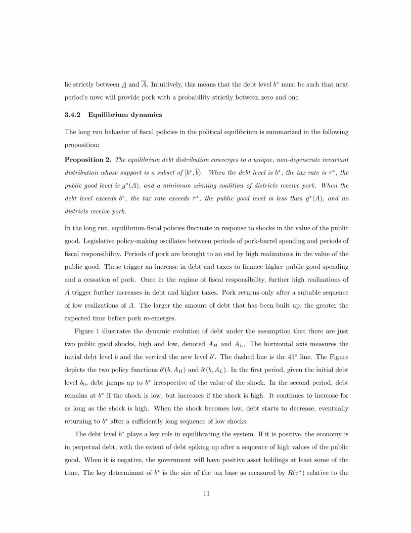
based on institutional considerations, we decided to infer q from the data. We choose to calibrate

bu because setting it equal to the theoretical upper bound on debt b = maxτ R(τ)/ρ creates

difficulties matching all the moments. In particular, the average debt/GDP ratio predicted by

the model is too high. We think that this reflects the fact that the theoretical upper bound is

unrealistically high. More specifically, since repaying b would imply setting all future public good

provision equal to zero, we suspect that the government would in fact default if saddled with this

amount of debt. We are not sure what is the true maximum amount the government could borrow

and so, again, we try to infer it from the data.

We choose our five parameters to match five target moments in the data. The first two targets

are the peacetime (i.e., excluding the WWII years) mean and variance of government spending as

a proportion of GDP in the U.S. during the period 1940-2005. The third is the maximum value of

government spending as a proportion of GDP. The final two are the average and maximum ratio

of government debt to GDP during 1940-2005.13 Our five parameters are chosen so that the

model generates, under the stationary distribution, close to the same values that are observed in

the data. The resulting values, together with other relevant parameters, are listed in Table 1.

n δ ε w p μ μw θ q bu

100 0.95 2 0.72 1 -1.05 -0.12 0.13 55.2 91.7

Table 1: Model Parameters

4.3 Model fit

Table 2 summarizes the model’s fit for a set of selected variables that compose the government’s

budget. The first column reports government spending as a percentage of GDP during peacetime

(GSp/GDP), while the second column includes the war years (GS/GDP). The third column reports

the ratio of government debt to GDP (GD/GDP), while the fourth reports government revenue

as a proportion of GDP (GR/GDP). In our model, the latter is simply the proportional income

tax rate τ .

13 All the moments used in the calibration are constructed from the dataset contained in “Historical Statistics ofthe United States”, Millennial Edition, Cambridge University Press (2008). The series for the ratio of governmentspending to GDP is constructed from the Treasury series (which ranges from 1789 to 1970) and the OMB series(ranging from 1940 to 2005), and includes Total Federal Expenditures, net of interest payments (all as a fractionof GDP). The measure of Total Expenditures includes Defense, Social Security and Veteran’s Compensations (so“mandatory” expenditures will be taken into account when calibrating average spending). The series of governmentdebt corresponds to Federal Public Debt.

15

The top two rows report the model’s simulated means and variances, and the bottom two rows

their counterparts in the data. The model’s statistics are based on a numerical approximation to

the theoretical invariant distribution of debt.14 The mean and standard deviation of peacetime

spending as a ratio of GDP (listed in bold in the first column), as well as the mean debt/GDP

ratio (listed in bold in the third column), are three of our five target values, and thus match the

data well by construction.

GSp/GDP GS/GDP GD/GDP GR/GDP=τ

Model Mean 17.37% 18.43% 56.98% 21%

Stdev 2.33% 5.40% 18% 1%

Data Mean 17.36% 18.18% 56.19% 17%

Stdev 2.32% 5.49% 20% 3%

Table 2: Model Simulation vs Data

The mean government spending/GDP ratio during WWII was also one of our target moments.

The model delivers 40.5% while the data counterpart is 40%. Note that the mean of government

spending/GDP (second column) predicted by the model matches the data well. Since this mean is

a combination of the two conditional means (peacetime and wartime), with the weights determined

by the probability of war, this suggests that our approximation of the shock process is accurate.

Consistent with tax smoothing principles, we see from Table 2 that the volatility of the gov-

ernment debt/GDP ratio in the data is much higher than that of the government revenue/GDP

ratio (20% for the former, 3% for the latter). Despite the fact that we did not directly target the

debt/GDP volatility, the model generated a value quantitatively similar to that observed in the

data. The predicted volatility of revenue/GDP is much lower than in the data suggesting that

there is more tax smoothing going on in the model than in the actual economy. Nonetheless, the

average revenue/GDP ratio generated by the model is very much in line with the data.

There are two other statistics not reported in Table 2 that are nonetheless important to men-

tion. The first one, is the targeted maximum debt/GDP ratio. The model delivers an expected

value of the maximum debt/GDP ratio of 120.6%, very close to the 121% observed in the data.

14 Using the theoretical distribution approach resulted in more robust estimates of the moments than the alter-native of simulating the economy for a given length of time.

16

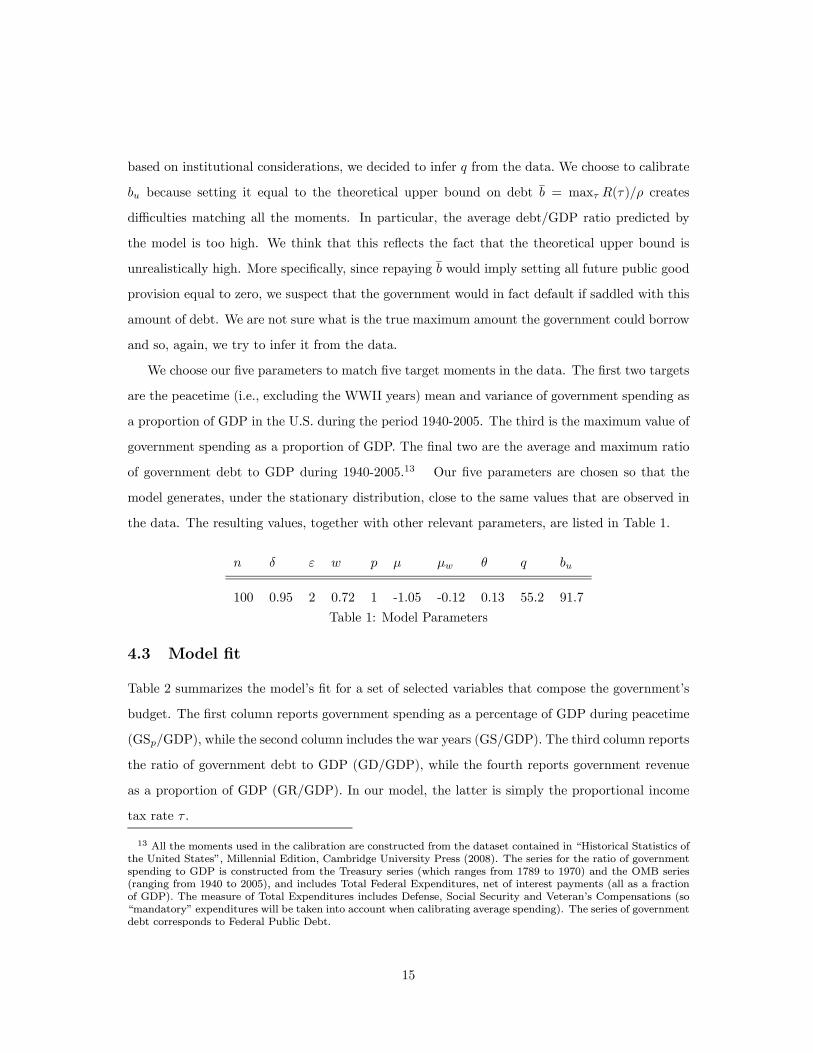
The second statistic, not a target value, is the lower bound on the debt/GDP ratio. In the data,

during the period 1940-2005 this was never below 31.5%. Encouragingly, the lower bound gen-

erated by the model–calculated as b∗/E(y)–is 29.4%. Thus, the political frictions captured by

the model generate quantitatively a realistic and endogenous lower bound for debt. Moreover,

the long-run stationary distribution of debt/GDP that our model generates is in line with that

observed in the U.S. as seen in Figure 2.

0.3 0.4 0.5 0.6 0.7 0.8 0.9 1 1.10

0.02

0.04

0.06

0.08

0.1

0.12

0.14

0.16

0.18

b/y

p

Histogram US debt/GDP

ModelUS Data

Figure 2: Stationary distribution of debt/GDP

The fact that the model delivers such a good fit with the actual distribution of the debt/GDP

ratio should not be overlooked. It is very difficult to explain the observed debt distribution with

a normative model. As noted earlier, the planner’s solution converges to a steady state where

the government has sufficient assets to finance the Samuelson level of the public good with the

interest earnings and taxes are zero. Obviously such a prediction is untenable. Aiyagari et. al

(2002) showed that a non-degenerate distribution for debt could be generated by imposing an

ad-hoc lower bound on debt (i.e., an upper limit on how many assets the government could hold).

However, as they observe, it is not clear why the government should face such a constraint. The

BC model provides a theoretical resolution of this difficulty and our calibration shows that, for

the U.S., this resolution works rather nicely empirically.

17

4.4 Simulations

To test how well the model captures the behavior of the key policy variables, we simulated the

economy for the period 1940-2005. As an initial condition, we assumed that debt/GDP in the

model was identical to that in the data. We further assumed that the economy was in peace until

1942, where we hit the system with a “war” shock for three years. After that, we assume the

economy remains in peace for the remainder of the sample. Given the initial value of b and the

sequence of shocks, we computed the evolution of government spending, revenues, and debt.

The left hand panel of Figure 3 shows the time paths of spending and revenue as a proportion

of GDP in the data. Revenues are much more stable than spending reflecting the government’s

tax smoothing. The right hand side show the impulse-responses from the model. The Figure

shows the model nicely replicates the tax smoothing behavior observed in the data.

1940 1950 1960 1970 1980 1990 20000.05

0.1

0.15

0.2

0.25

0.3

0.35

0.4

0.45

time

% o

f GDP

US Data

1940 1950 1960 1970 1980 1990 20000.1

0.15

0.2

0.25

0.3

0.35

0.4

time

% o

f GDP

Model

revenues

s pend ing

revenues

s pending

Figure 3: Response to a war shock, data (left panel) vs model (right panel)

The U.S. government financed the massive increase in public spending during the war years

largely by issuing debt. The increase in the government debt/GDP ratio can be seen in Figure 4,

which also depicts the behavior of debt for our simulated economy. Notice that the model captures

the jump in debt very well. Another interesting thing to note is that while government spending

decreased rapidly after the shock, the level of debt drops back at a much lower speed. While we

capture this qualitatively, our model over-predicts debt persistence. The model also has difficulty

18

in explaining the up-turn in the debt/GDP ratio in the 1980s and 1990s. We suspect that there

was a structural shift in the willingness to run deficits which is not picked up by the model.

1940 1950 1960 1970 1980 1990 2000 2010

0.4

0.5

0.6

0.7

0.8

0.9

1

1.1

1.2

year

% o

f GD

P

US data

Model

Figure 4: Response of debt to a war

4.5 Some limitations

We feel that the calibrated BC model provides a surprisingly good fit of the data given its sim-

plicity. In particular, the fit of the debt distribution illustrated in Figure 2 is very encouraging.

This provides some justification for using the model to analyze how imposing a balanced budget

amendment would impact the U.S. economy. Nonetheless, the model has many limitations and

we discuss three of the most important ones here.

Although dynamic, the BC model does not allow for persistent growth. Since there has been

substantial growth in the U.S. economy over the period in question, to calibrate the model it

is necessary to match the predictions of the model concerning policies as a proportion of GDP

with the data on policies as a proportion of GDP. Matching policy levels, even when corrected for

inflation, would not be possible. But this raises the question of whether the equilibrium behavior of

fiscal policies that the model predicts would emerge in a growing economy. For example, would the

debt/GDP ratio in a growing economy behave the same as the debt/GDP ratio in the stationary

economy? This is an open question.

A second limitation concerns entitlements spending. We included Social Security and Medicare

19

spending in our computation of the government spending/GDP ratio. Expenditure on these

programs has grown significantly since WWII and this is primarily responsible for the upward

trend in the spending/GDP ratio exhibited in the left panel of Figure 3. In calibrating the model,

we target the average spending/GDP ratio over the entire 1940-2005 period. Thus, our shock

structure does not incorporate the increase in spending observed in the latter part of our sample

period.

A third limitation concerns the assumed constant marginal utility of consumption. This as-

sumption means that, given the interest rate ρ, citizens are indifferent over the time path of their

consumption. This results in consumption being more volatile in the model than in the data.15

The assumption also implies that the interest rate is constant so that the model cannot capture

variations in interest rates.16

5 The impact of a strict BBR

We are now ready to analyze the impact of imposing a strict BBR on the economy. We model a

strict BBR as a requirement that tax revenues must always be sufficient to cover spending and

the costs of servicing the debt. If the initial level of debt is b, this requires that

R(τ) ≥ pg +Xi

si + ρb. (11)

Given the definition of B(τ, g, b0; b) (see (3)), a BBR is equivalent to adding, in each period, the

feasibility constraint that b0 ≤ b; i.e., that debt cannot increase. Thus, under a BBR, next period’s

feasible debt levels are determined by this period’s debt choice. In particular, if debt is paid down

in the current period, that will tighten the debt constraint in the next period. We first study what

can be said qualitatively about the impact of a BBR and then turn to the calibrated model.

5.1 Qualitative analysis

Under a BBR, the equilibrium will still have a recursive structure. Let {τc(b,A),gc(b,A),b0c(b,A)}

denote the equilibrium policies under the constraint and vc(b,A) the value function. As in the

15 The standard deviation of consumption as a proportion of GDP is 5.4% in the model and 3.8% in the data.

16 In addition, with a diminishing marginal utility of consumption, the government will have incentives tomanipulate the interest rate in its favor. Given a lack of commitment, this would cause further distortions in apolitical equilibrium. For a discussion of this, see Lucas and Stokey (1983) for the benevolent planner case, andAzzimonti, deFrancisco and Krusell (2007) for an analysis under majority voting.

20

unconstrained equilibrium, in any given state (b,A), either the mwc will provide pork to the

districts of its members or it will not. If the mwc does provide pork, it will choose a tax-public

good-debt triple that maximizes coalition aggregate utility under the assumption that they share

the net of transfer surplus. Thus, (τ, g, b0) solves the problem:

maxu(τ) +A ln g + B(τ,g,b0;b)q + δEvc(b

0, A0)

s.t. b0 ≤ b.

The optimal policy is (τ∗, g∗(A), b∗c(b)) where the tax rate τ∗ and public good level g∗(A) are as

defined in (5) and (6), and the public debt level b∗c(b) satisfies

b∗c(b) ∈ argmax{b0

q+ δEvc(b

0, A0) : b0 ≤ b}. (12)

As in the case without a BBR, if the mwc does not provide pork, the outcome will be as if it

is maximizing the utility of the legislature as a whole. Following the logic of Proposition 1, we

obtain:

Proposition 3. Under a strict BBR, the equilibrium value function vc(b,A) solves the functional

equation

vc(b,A) = max(τ,g,b0)

⎧⎪⎪⎨⎪⎪⎩u(τ) +A ln g + B(τ,g,b0;b)

n + δEvc(b0, A0) :

B(τ, g, b0; b) ≥ 0, τ ≥ τ∗, g ≤ g∗(A), & b0 ∈ [b∗c(b), b]

⎫⎪⎪⎬⎪⎪⎭ (13)

and the equilibrium policies {τc(b,A),gc(b,A),b0c(b,A)} are the optimal policy functions for this

program.

As in Proposition 1, the equilibrium can be expressed as a particular constrained planner’s

problem. There are two key differences created by the BBR. First, there is an additional constraint

on debt - an upper bound, b0 ≤ b. Second, the endogenous lower bound on debt b∗c(b) will be a

function of b. Because of these two features, the set of feasible policies is now state dependent as

well as endogenous. Determining the shape of the function b∗c(b) will be crucial to the analysis of

the dynamics and the steady state of the equilibrium. Before turning to this, however, note that

we can use Proposition 3 to characterize the equilibrium policies for a given function b∗c(b). If A is

less than A∗(b, b∗c(b)) the tax-public good-debt triple is (τ∗, g∗(A), b∗c(b)) and the mwc shares the

net of transfer surplus B(τ∗, g∗(A), b; b∗c(b)). If A is greater than A∗(b, b∗c(b)) the budget constraint

binds and no transfers are given. The tax rate exceeds τ∗, the level of public good is less than

21

g∗(A), and the debt level exceeds b∗c(b). In this case, the solution can be characterized by solving

problem (13) with only the budget constraint binding and the constraint that b0 ≤ b.

5.1.1 Characterization of the function b∗c(b)

The function b∗c(b) tells us, for any given initial b, the debt level that the mwc will choose when

it provides pork. To understand what b∗c(b) is, it is first useful to understand what it cannot be.

Suppose that the expected value function Evc(b,A0)were strictly concave (as is the case without

a BBR). Then the objective function of the maximization problem in (12) would also be strictly

concave and there would be a unique bb such that b∗c(b) = min{bb, b}. Thus, for any b larger thanbb, whenever the mwc chooses to provide pork, it would choose the debt level bb. If this were thecase, however, a contradiction would emerge. To see why, note that for initial debt levels b belowbb, the BBR would always be binding so that b0c(b,A) = b for all A. On the other hand, for debt

levels above bb, there will be states A in which the BBR will not bind so that b0c(b,A) < b. This

means that when b is below bb, a marginal reduction of debt would be permanent: all future mwcswould reduce debt by the same amount. By contrast, for b above bb, a marginal reduction in debtwould have an impact on the following period, but it would affect the remaining periods only in

the states in which the BBR is binding. Indeed, when the BBR is not binding, b∗c(b) would equalbb, and so would be independent of b. It follows that the marginal benefit of reducing debt to theleft of bb would be higher than the marginal benefit of decreasing debt to the right of bb. But thiscontradicts the assumption that the expected value function Evc(b,A

0) is strictly concave.

The essential problem with a b∗c(b) function of the form min{bb, b} is that the marginal effectof b on b∗c(b) changes too abruptly at

bb, from one to zero. In equilibrium, the debt level the mwc

chooses when it provides pork and the BBR is not binding must change more smoothly. This is not

possible when the expected value function is strictly concave, because the maximization problem in

(12) has a unique solution which allows no flexibility in choosing b∗c(b). If the equilibrium expected

value function is concave, therefore, it must be weakly concave. Weak concavity does not pose

the same problem since it allows for the possibility that there are a range of debt levels that solve

the maximization problem in (12). Suppose this is the case and let b0 denote the smallest of these

and b1 the largest; that is,

b0 = min argmax{b0

q+ δEvc(b

0, A0)}, (14)

22

and

b1 = maxargmax{b0

q+ δEvc(b

0, A0)}. (15)

Then any point in [b0, b1] will solve the maximization problem in (12). If the initial debt level b

is smaller than b0, then we must have b∗c(b) = b. But if the initial debt level b exceeds b0 then the

associated b∗c(b) could be any point in the interval [b0,min{b, b1}]. This extra flexibility suggests

that there may exist a function b∗c(b) which guarantees that the expected value function is indeed

weakly concave. Fortunately, this is not only the case, but there exists a unique such function.

To make all this more precise, define an equilibrium under a strict BBR to be well-behaved

if (i) the expected value function is concave and differentiable everywhere, and (ii) the function

b∗c(b) is non-decreasing and differentiable everywhere. In addition, let (τb(A), gb(A)) be the tax

rate and public good level that solve the static maximization problem

max(τ,g)

½u(τ) +A ln g +

B(τ, g, b, b)

n: B(τ, g, b, b) ≥ 0

¾. (16)

Then we have:

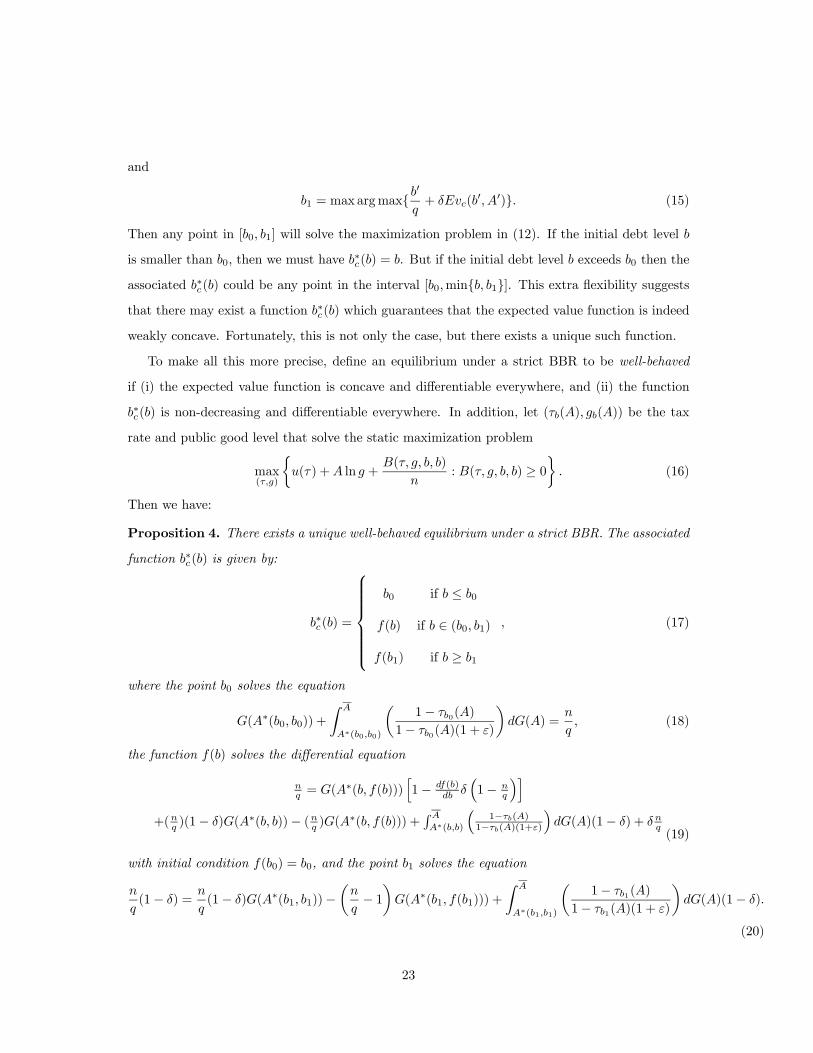
Proposition 4. There exists a unique well-behaved equilibrium under a strict BBR. The associated

function b∗c(b) is given by:

b∗c(b) =

⎧⎪⎪⎪⎪⎪⎪⎨⎪⎪⎪⎪⎪⎪⎩b0 if b ≤ b0

f(b) if b ∈ (b0, b1)

f(b1) if b ≥ b1

, (17)

where the point b0 solves the equation

G(A∗(b0, b0)) +

Z A

A∗(b0,b0)

µ1− τb0(A)

1− τb0(A)(1 + ε)

¶dG(A) =

n

q, (18)

the function f(b) solves the differential equation

nq = G(A∗(b, f(b)))

h1− df(b)

db δ³1− n

q

´i+(nq )(1− δ)G(A∗(b, b))− (nq )G(A∗(b, f(b))) +

R AA∗(b,b)

³1−τb(A)

1−τb(A)(1+ε)

´dG(A)(1− δ) + δ nq

(19)

with initial condition f(b0) = b0, and the point b1 solves the equation

n

q(1− δ) =

n

q(1− δ)G(A∗(b1, b1))−

µn

q− 1¶G(A∗(b1, f(b1))) +

Z A

A∗(b1,b1)

µ1− τb1(A)

1− τb1(A)(1 + ε)

¶dG(A)(1− δ).

(20)

23

Proof: See Appendix.

The function b∗c(b) is tied down by the requirement that the objective function in the maxi-

mization problem (12) must be constant on the interval [b0, b1]. In a well-behaved equilibrium,

this implies that −δE∂vc(b0, A0)/∂b0 = 1/q. Since the derivative of the expected value function

depends upon the function b∗c(b) and its derivative, this implies that b∗c(b) satisfies a differential

equation with appropriate end-point conditions. This differential equation and its end-points are

spelled out in Proposition 4 and derived in its proof.

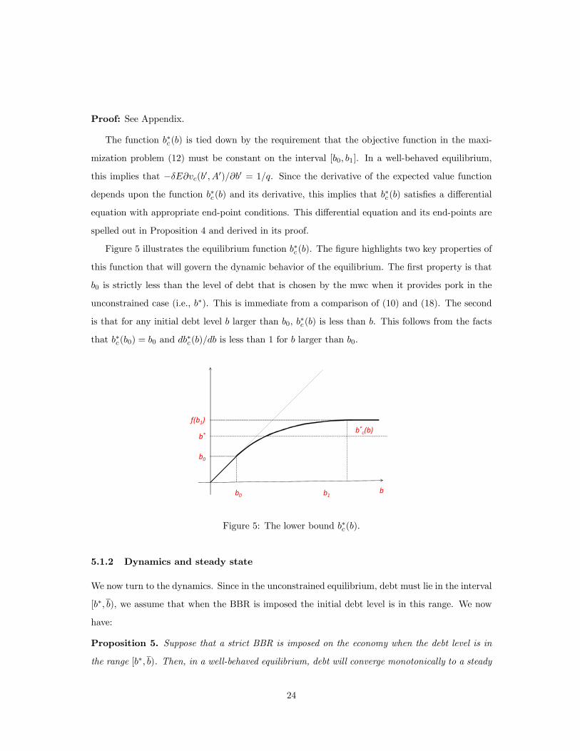
Figure 5 illustrates the equilibrium function b∗c(b). The figure highlights two key properties of

this function that will govern the dynamic behavior of the equilibrium. The first property is that

b0 is strictly less than the level of debt that is chosen by the mwc when it provides pork in the

unconstrained case (i.e., b∗). This is immediate from a comparison of (10) and (18). The second

is that for any initial debt level b larger than b0, b∗c(b) is less than b. This follows from the facts

that b∗c(b0) = b0 and db∗c(b)/db is less than 1 for b larger than b0.

b0

b0

b*

f(b1)

b1 b

b*c(b)

Figure 5: The lower bound b∗c(b).

5.1.2 Dynamics and steady state

We now turn to the dynamics. Since in the unconstrained equilibrium, debt must lie in the interval

[b∗, b), we assume that when the BBR is imposed the initial debt level is in this range. We now

have:

Proposition 5. Suppose that a strict BBR is imposed on the economy when the debt level is in

the range [b∗, b). Then, in a well-behaved equilibrium, debt will converge monotonically to a steady

24

Figure 6: Evolution of debt under a BBR

state level b0 smaller than b∗. At this steady state level b0, when the value of the public good is less

than A∗(b0, b0), the tax rate will be τ∗, the public good level will be g∗(A), and a mwc of districts

will receive pork. When the value of the public good is greater than A∗(b0, b0), the tax rate will be

τb0(A), the public good level will be gb0(A), and no districts will receive pork.


To understand this result, note first from Propositions 3 and 4 that b0c(b0, A) = b0 for all A

so that b0 is a steady state. The key step is therefore to show that the equilibrium level of debt

must converge down to the level b0. Since debt can never increase, this requires ruling out the

possibility that debt gets “stuck” before it gets down to b0. This is done by showing that for

any debt level b greater than b0, the probability that debt remains at b converges to zero as the

number of periods goes to infinity.

Figure 6 illustrates what happens to debt in the two shock case depicted in Figure 1. The

Figure depicts the two policy functions b0c(b,AH) and b0c(b,AL). When the shock is high, the

constraint that debt cannot increase is binding and hence b0c(b,AH) = b for all b ≥ b0. When the

shock is low, however, the constraint is not binding and the mwc finds it optimal to pay down

debt. Given an initial debt level exceeding b∗, debt remains constant as long as the shock is high.

When the shock is low, debt starts to decrease. Once it has decreased, it can never go up because

25

of the BBR constraint. Debt converges down to the new steady state level of b0.

We can now use Proposition 5 to compare policies at the new steady state with long run

policies in the unconstrained equilibrium.

Proposition 6. At the steady state debt level b0, the average primary surplus is lower than the

long run average primary surplus in the unconstrained equilibrium. In addition, the average level

of pork-barrel spending is higher.


Recall that the primary surplus is the difference between tax revenues and public spending other

than interest payments. Thus, the first part of this result implies that steady state average tax

revenues must be lower under a BBR and/or average public spending must be higher. It should be

stressed, however, that this result only refers to the long run. In the transition to the new steady

state, at least initially, taxes will be higher and public good spending will be lower as revenues

are used to reduce debt.

The above analysis provides a reasonably complete picture of how imposing a BBR will impact

fiscal policy. However, we are also interested in the impact on citizens’ welfare. When it is first

imposed, it seems likely that a BBR will reduce contemporaneous utility. When A is low, instead

of transfers being paid out to the citizens, debt will be being paid down. When A is high, the

increase in taxes and reduction in public goods will be steeper than would be the case if the

government could borrow. Thus, in either case, citizen welfare should be lower. As debt falls, the

picture becomes less clear. On the one hand, citizens gain from the higher average public spending

levels and/or lower taxes resulting from the smaller debt service payments. On the other hand,

the government’s ability to smooth tax rates and public good levels by varying the debt level is

lost. Thus, there is a clear trade-off whose resolution will depend on the parameters. The welfare

issue is therefore fundamentally a quantitative question and to resolve it we need to turn to the

calibrated model.

5.2 Quantitative analysis

The computation of the equilibrium is much easier with a strict BBR than without because the

function b∗c(b) can be directly solved for. To see this, note that the steady state value of debt

b0 can be computed directly from equation (18), since the tax function τb(A) can be obtained

by solving the static problem (16). Given this, the function f(b) can be found immediately by

26

solving the differential equation (19) with initial condition f(b0) = b0, and the end point b1 can

be found using equation (20).17 Once the function b∗c(b) is obtained, policy and value functions

can be computed following Step 2 in the algorithm described above (with the exception that the

constraint on debt is replaced by b0 ∈ [b∗c(b), b]). For the calibrated economy, we find that b0 = 5.9,

a significantly lower value than b∗, which was 29.4.

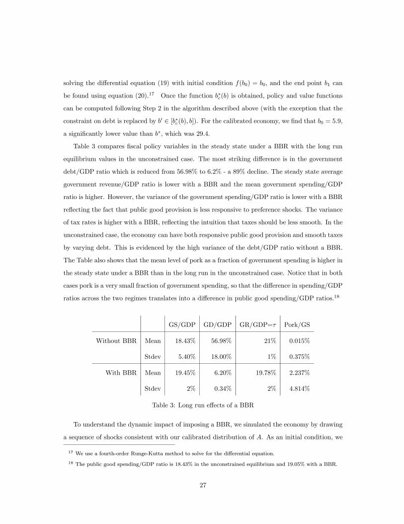
Table 3 compares fiscal policy variables in the steady state under a BBR with the long run

equilibrium values in the unconstrained case. The most striking difference is in the government

debt/GDP ratio which is reduced from 56.98% to 6.2% - a 89% decline. The steady state average

government revenue/GDP ratio is lower with a BBR and the mean government spending/GDP

ratio is higher. However, the variance of the government spending/GDP ratio is lower with a BBR

reflecting the fact that public good provision is less responsive to preference shocks. The variance

of tax rates is higher with a BBR, reflecting the intuition that taxes should be less smooth. In the

unconstrained case, the economy can have both responsive public good provision and smooth taxes

by varying debt. This is evidenced by the high variance of the debt/GDP ratio without a BBR.

The Table also shows that the mean level of pork as a fraction of government spending is higher in

the steady state under a BBR than in the long run in the unconstrained case. Notice that in both

cases pork is a very small fraction of government spending, so that the difference in spending/GDP

ratios across the two regimes translates into a difference in public good spending/GDP ratios.18

GS/GDP GD/GDP GR/GDP=τ Pork/GS

Without BBR Mean 18.43% 56.98% 21% 0.015%

Stdev 5.40% 18.00% 1% 0.375%

With BBR Mean 19.45% 6.20% 19.78% 2.237%

Stdev 2% 0.34% 2% 4.814%

Table 3: Long run effects of a BBR

To understand the dynamic impact of imposing a BBR, we simulated the economy by drawing

a sequence of shocks consistent with our calibrated distribution of A. As an initial condition, we

17 We use a fourth-order Runge-Kutta method to solve for the differential equation.

18 The public good spending/GDP ratio is 18.43% in the unconstrained equilibrium and 19.05% with a BBR.

27

assumed that the government debt/GDP ratio equalled 63% which was the level prevailing in the

U.S. in 2005, the last year for which we have data. It took around 70 periods for the economy

to transition to a debt level below b∗ (the equivalent of about a 30% debt/GDP ratio), with the

convergence to the new steady state (about a 6% debt/GDP ratio) occurring at a much slower

speed. Figure 7 compares the dynamics of fiscal policy with and without a BBR. As can be seen in

the first panel of Figure 7, in the unconstrained case (the red dotted line) the government always

issues debt in time of war: with a BBR, however, it is forced to have zero deficits. This induces a

marked downward drift in the evolution of debt.

0 50 1000

20

40

60

80

100

tim e

Debt

D e b t

0 50 1000

0.2

0.4

0.6

0.8

1

1.2

tim e

Debt

/GDP

D e b t/G D P

0 50 1000.18

0.2

0.22

0.24

0.26

0.28

0.3

tim e

Taxe

s

Ta xe s

0 50 1000

10

20

30

40

tim e

Expe

nditu

res

E xp e n d i tu re s

Figure 7: Evolution of key variables (- - red benchmark, — blue BBR )

The second panel of Figure 7 measures the debt/GDP ratio. Note that this measure spikes

during war-time even with a BBR. The reason is that, even though debt remains constant, GDP

goes down due to the increase in taxation needed to finance the war. The spike in taxes during war

time under a BBR is clearly illustrated in the third panel of Figure 7 which nicely illustrates the

negative consequences of a BBR for tax smoothing. On the other hand, the panel also illustrates

28

how a BBR serves to lower average tax rates over time. The fourth and final panel of Figure 7

illustrates that public good provision is much less responsive with a BBR. However, the average

level of public good provision rises above the level of provision without a BBR as debt converges

to the new steady state.

Figure 8 looks at the evolution of pork and debt under a BBR. Pork is not provided when the

BBR is initially imposed but is provided with increasing frequency as debt levels decline.

0 50 100 150 200 250 300 350 400 450 50010

15

20

25

30

35

40

45

50

55

60

0 50 100 150 200 250 300 350 400 450 5000

0.5

1

1.5

2

2.5

3

3.5

4

4.5

5

time$

Evolution of Pork and debt

Figure 8: Pork under a BBR

Steady state welfare under a strict BBR, as measured by Evc(b0, A), is 2.85% higher than the

corresponding long run value without a BBR.19 . This welfare gain reflects the lower cost of debt

service at the new steady state. However, as discussed above, the fact that steady state welfare is

higher does not mean that imposing a BBR will raise welfare because of the costs incurred in the

transition to the new steady state. Figure 9 illustrates the evolution of contemporaneous utility

following the imposition of a BBR. In the first 40 periods, contemporaneous welfare is most of

the time lower under a BBR. However, after the first war shock, debt is sufficiently lower under a

BBR that contemporaneous welfare overtakes that in the unconstrained equilibrium and exceeds

it thereafter even during war time.20 While this is not obvious from the Figure, the short run

19 Long run welfare without a BBR is given byRbEv(b,A)dψ(b) where ψ(b) is the stationary distribution of debt.

20 The fact that contemporaneous utility spikes up in war time is just an artifact of how we have modelled waras an increase in the value of public goods. There are obviously other utility costs of war that are not accountedfor by the model.

29

0 10 20 30 40 50 60 70 80 90 100

1

1.5

2

2.5

3

3.5

time

Wel

fare

Evolution of Instantaneous Utility

Figure 9: The evolution of welfare (- - red benchmark, — blue BBR)

costs are sufficiently high that imposing a BBR given the level of debt in the U.S. in 2005 (our

last year of data) will actually reduce welfare. Moreover, this is true for any initial debt level in

the support of the long run distribution in the unconstrained equilibrium.

While the question is purely academic, one can use the calibrated model to ask whether the

U.S. would have been better off at its founding banning deficits, that is if a strict BBR were

imposed at the beginning of time before the government had accumulated any debt. Assuming

that initial debt equals zero and that b0 (as defined in (18)) exceeds 0, under such a BBR, debt

would remain at 0 forever. Thus, we can quantify the welfare gains of introducing a BBR at

foundation by comparing Evc(0, A) and Ev(0, A) in the calibrated economy.21 We find that such

a ban would have increased welfare by 0.017%.

21 This comparison is the one analyzed in Battaglini and Coate (2008). They prove that if R(τ∗) exceeds pg∗(A),then it must be the case that Evc(0, A) exceeds Ev(0, A) and a BBR is welfare improving. To see the logic, notethat the condition implies that A∗(0, 0) exceeds A and hence the tax-public good pair would always be (τ∗, g∗(A))under a BBR. But without a BBR, by Proposition 2, the tax rate would never be lower than τ∗ and sometimeswould be strictly higher and the public good level would never be higher than g∗(A) and sometimes would bestrictly lower. Thus, citizens must be better off with a BBR. This condition, however, is quite restrictive and isnot satisfied in our calibrated economy.

30

6 Impact of a BBR with super-majority override

Now consider the impact of a BBR that can be overruled with the support of q0 > q legislators.

Thus, if the proposer can obtain the support of q0 legislators, he can pass a proposal which runs

a deficit and raises the debt level. Otherwise, the rule binds. Of course, if the proposer is not

planning to raise debt, then he only needs the support of q legislators to pass his proposal. We

now have the following striking result.

Proposition 7. Suppose that a BBR with super-majority override is imposed on the economy

when the debt level is at least b∗. Then the rule will have no effect on fiscal policies and citizens’

welfare.

The logic underlying this result is straightforward. In the long run equilibrium of the uncon-

strained model, a mwc never simultaneously runs a deficit and provides pork. This follows from

the fact that when a mwc provides pork it chooses the debt level b∗ which is the lowest level of debt

in the support of the long run distribution. Thus, whenever the mwc runs a deficit it is effectively

behaving as a planner would and its proposal is therefore supported unanimously. Requiring the

mwc to obtain additional support for its deficit-financed proposal therefore imposes no constraint

on its behavior.

When reflecting on this result, it is important to note that if a BBR with override were

imposed on the economy before debt had risen to equilibrium levels, it would have an effect. This

is because it will constrain the initial surge in deficit-financed pork which increases debt to b∗ and

will therefore shift the debt distribution to the left. The greater the required super-majority, the

larger the shift. This leftward shift in the debt distribution would likely enhance social welfare.

7 Discussion

Our analysis offers a clear account of the social costs and benefits of imposing a strict BBR. The

social cost is less responsive public good provision and greater volatility in tax rates. The inability

to run deficits means that the only way to respond to positive shocks in the value of the public

good is to raise taxes. This leads to sharper tax hikes. Moreover, since the marginal cost of public

funds is higher, public good provision incentives are dampened. The social benefit of a strict BBR

is that the level of debt is reduced. While this reduction imposes short run costs, in the long

run citizens benefit since debt starts out inefficiently high. The lower debt burden permits higher

31

average levels of public goods and lower taxes.

This account of the social cost of a strict BBR is consistent with the policy debate. The

major drawback of a balanced budget amendment to the U.S. constitution stressed by opponents

is that it reduces the federal government’s ability to deal with emergency spending needs and/or

unexpected revenue shortages. Emergency spending needs include wars, natural disasters, and the

need to pump-prime the economy in recessions.22 Revenue shortages come from business cycle

fluctuations. The inability of the government to run deficits in these circumstances is predicted

to lead to inadequate federal spending and/or excessive taxation.23

The account of the social benefit of a strict BBR is also consonant with the policy debate.

Advocates of a balanced budget amendment certainly see the main goal as being to reduce the

debt burden on the economy. However, the advantage of our analysis is that it spells out an

explicit mechanism by which debt reduction occurs. The analysis is also useful in clarifying what

happens to government taxes and spending. Many advocates seem to assume that a balanced

budget amendment will lead to smaller government. If the size of government is measured by the

tax rate, then our calibrated model suggests that on average this is true (see Table 3). Nonetheless,

average spending on both public goods and pork will in fact increase. This suggests that if the true

goal of a BBR is to reduce government spending, it should be supplemented by tax or spending

limits.

The force leading to debt reduction in our analysis is that a BBR, by restricting future policies,

increases the expected cost of taxation and increases legislators’ incentive to save. It is worth

noting that, in a growing economy, there will be an additional, purely mechanical, force driving

down the debt/GDP ratio. A strict BBR, by banning deficits, amounts to a constraint that the

current level of debt cannot exceed the initial level.24 Accordingly, if GDP is growing, the

debt/GDP ratio must fall even if debt is constant. Exactly how this force will combine with

the force identified by our analysis is an open question, but the direction of the overall effect is

22 Typically, however, the amendments considered by the U.S. Congress specify that the BBR is to be automat-ically waived in times of war.

23 Inadequate spending tends to be emphasized because the view is that political opposition to tax hikes willbe higher than to spending cut-backs. This reflects the fact that federal spending programs are often targeted toparticular sub-groups of the population, while taxes are paid by a broader group of citizens. In our model, allcitizens are homogeneous in their preferences over public good provision and taxes and therefore these are alwayskept in balance.

24 This is as opposed to a constraint that today’s debt/GDP ratio cannot exceed tomorrow’s. In some sense, aconstraint that the debt/GDP ratio cannot grow seems a more natural rule to propose for a growing economy thana BBR (as argued by Paget (1996)). However, we are not aware of any serious proposal for such a rule.

32

unambiguous.

Our quantitative assessment of the relative size of the social costs and benefits is, of course,

highly model dependent. It is interesting to give a sense of the strength of the forces at work, but it

is not intended to be definitive. It is easy to think of factors that could substantially increase both

the costs and the benefits of a BBR. On the cost side, if Keynesian pump-priming could prevent

recessions from deepening, then cramping the federal government’s ability to engage in it might

indeed be very costly. On the benefit side, if reducing government debt would decrease interest

rates and spur private investment and growth, then the benefits of government debt reduction

could be much greater than suggested by our model.25

Imposing a BBR with super-majority override will have no effect according to our analysis.

This conclusion reflects the fact that once debt is at equilibrium levels, deficits are used to finance

only public good spending and not targeted pork. They are therefore supported unanimously.

Thus, while the equilibrium level of debt is excessive, deficits are, in a sense, not excessive in long

run equilibrium. We suspect that this feature reflects the stationary nature of the underlying

economy and would not be robust to including growth. In a growing economy, the debt level will

likely grow over time even when the mwc is providing pork. Thus, rather than being an absolute

level of debt, b∗ would be the debt/GDP ratio that is chosen when the mwc provides pork. If

GDP is increasing, then in order to maintain the debt/GDP ratio at b∗, the mwc will have to

issue new debt and thereby run a deficit. But if the mwc needs super-majority approval to run

a deficit, then it may be constrained in its ability to do so. Accordingly, we expect a BBR with

override might have an effect. Of course, exactly what this effect will be is an open question.

Given the possible non-robustness of our result to introducing growth, we must be cautious in

treating it as a definitive prediction. Nonetheless, we do feel that the result is useful in focusing

attention on the question of exactly how a BBR is supposed to make a difference when it can be

overridden by a super-majority of legislators. Advocates of a balanced budget amendment usually

support an override to preserve some flexibility, but implicitly assume that a requirement to get

the support of, say, 3/5ths of both Houses of Congress will have bite. Indeed, the discussion tends

to focus on the concern that such a requirement might be too stringent and could lead to hold up

problems with legislators demanding special projects for their districts in exchange for their votes.

25 That said, these considerations would impact the equilibrium level of debt in the unconstrained case so thatthe change created by the BBR might be much less dramatic. Of course, this is why an equilibrium analysis suchas ours is necessary to predict the impact of imposing a BBR.

33

The theoretical and/or empirical justification for these views is obscure and our result poses an

interesting challenge to them.

8 Conclusion

This paper has made a first attempt to analyze the impact of a balanced budget amendment to

the U.S. constitution. The framework for the analysis has been the political economy model of

fiscal policy recently developed by Battaglini and Coate (2008). The paper has calibrated the

BC model to the U.S. economy and has analyzed, qualitatively and quantitatively, the impact of

imposing two different types of BBRs: a strict rule that cannot be circumvented by the legislature

and a rule that can be overridden by a super-majority of legislators. We hope that the paper

has contributed to the policy debate on the case for a balanced budget amendment, as well as

advanced understanding of the strengths and weaknesses of the BC model as a framework for

analyzing U.S. fiscal issues.

We feel that the analysis offers a reasonably compelling vision of the likely impact of a strict

BBR. The key theoretical insight is that imposing a strict BBR will lead legislators to reduce

existing debt levels. By restricting future policies, a BBR increases the expected cost of taxation

and makes public savings more valuable. This reduction in debt has beneficial long run effects

because it reduces the revenues that must be devoted to servicing the debt. These beneficial effects

must be weighed against the costs of less responsive public good provision and more volatile tax

rates. While we are less satisfied with the prediction of the analysis concerning the (non) impact

of a BBR with a super-majority override, we do feel that it is useful in raising the question of

exactly how such a BBR is supposed to make a difference. This is an important question which

the policy debate has paid insufficient attention to.

In terms of future research, there is obviously much room for improvement in the analysis of

this important policy problem. In our view, the obvious next step is to extend the BC model to

include growth. Incorporating growth need not be done in a very sophisticated way to be valuable.

Assuming, for example, that labor productivity is growing exogenously over time would be a good

place to start. What is important is to preserve the tractability of the model and this will be a

major challenge. But, if a tractable extension can be crafted, it would be very interesting to use

it to revisit the case for a balanced budget amendment. We suspect that different conclusions

concerning the impact of a BBR with super-majority override would emerge.

34

References

Alt, J. and R. Lowry, (1994), “Divided Government and Budget Deficits: Evidence from theStates,” American Political Science Review, 88(4), 811-828.

Azzimonti, M., deFrancisco, E. and P. Krusell, (2007), “Production Subsidies and Redistri-bution,” Journal of Economic Theory, forthcoming.

Barro, R., (1979), “On the Determination of the Public Debt,” Journal of Political Economy,87, 940-971.

Bassetto, M. with T. Sargent, (2006), “Politics and Efficiency of Separating Capital andOrdinary Government Budgets,” Quarterly Journal of Economics, 121(4), 1167-1210.

Battaglini, M. and S. Coate, (2008), “A Dynamic Theory of Public Spending, Taxation andDebt,” American Economic Review, 98(1), 201-236.

Bayoumi, T. and B. Eichengreen, (1995), “Restraining Yourself: The Implications of FiscalRules for Economic Stabilization,” IMF Staff Papers, 42, 32-48.

Besley, T. and M. Smart, (2007), “Fiscal Restraints and Voter Welfare,” Journal of PublicEconomics, 91, 755-773.

Bohn, H. and R. Inman, (1996), “Balanced Budget Rules and Public Deficits: Evidencefrom the U.S. States,” Carnegie-Rochester Conference Series on Public Policy, 45, 13-76.

Braun, M., (1992), Differential Equations and their Applications, 4th Edition, New York:Springer-Verlag.

Brennan, G. and J. Buchanan, (1980), The Power to Tax: Analytical Foundations of a FiscalConstitution, Cambridge: Cambridge University Press.

Buchanan, J., (1995), “Clarifying Confusion about the Balanced Budget Amendment,” Na-tional Tax Journal, 48, 347-355.

Buchanan, J. and R. Wagner, (1977), Democracy in Deficit: The Political Legacy of LordKeynes, New York: Academic Press.

Chari, V.V., L. Christiano and P. Kehoe, (1994), “Optimal Fiscal Policy in a Business CycleModel,” Journal of Political Economy, 102(4), 617-652.

Cooley, T. and E. Prescott, (1995), “Economic Growth and Business Cycles,” in Cooley, T.ed, Frontiers of Business Cycle Research, Princeton: Princeton University Press.

Corsetti, G. and N. Roubini, (1996) “European and American Perspectives on Balanced-Budget Rules,” American Economic Review, 86(2), 408-413.

Greenwood, J., Z. Hercowitz and G. Huffman, (1988), “Investment, Capacity Utilization,and the Real Business Cycle,” American Economic Review, 78, 402-417.

Hall, G., J. Krieger and M. Gertler, (2000), “The Tax Smoothing Implications of the FederalDebt Paydown,” Brookings Papers on Economic Activity, 2, 253-301.

Hou, Y. and D. Smith, (2006), “A Framework for Understanding State Balanced BudgetRequirement Systems: Reexamining Distinctive Features and an Operational Definition,”Public Budgeting and Finance, 26(3), 22-45.

35

Inman, R., (1996), “Do Balanced Budget Rules Work? U.S. Experience and Possible Lessonsfor the EMU,” NBER Working Paper #5838.

Keech, W., (1985) “A Theoretical Analysis of the Case for a Balanced Budget Amendment,”Policy Sciences, 18, 157-168.

Lucas, R. and N. Stokey, (1983), “Optimal Fiscal and Monetary Policy in an Economywithout Capital,” Journal of Monetary Economics, 12, 55-93.

Marcet, A. and A. Scott, (2001), “Debt and Deficit Fluctuations and the Structure of BondMarkets,” mimeo, Universitat Pompeu Fabra.

Morgan, I., (1998), “Unconventional Politics: The Campaign for a Balanced-Budget Amend-ment Constitutional Convention in the 1970s,” Journal of American Studies, 32, 421-455.

Niskanen, W., (1992), “The Case for a New Fiscal Constitution,” Journal of EconomicPerspectives, 6(2), 13-24.

Paget, K., (1996), “The Balanced Budget Trap,” The American Prospect, 29, 21-29.

Poterba, J., (1994), “ State Responses to Fiscal Crises: The Effects of Budgetary Institutionsand Politics,” Journal of Political Economy, 102, 799-821.

Poterba, J., (1995), “Balanced Budget Rules and Fiscal Policy: Evidence from the States,”National Tax Journal, 48(3), 329-336.

Poterba, J., (1996), “Budget Institutions and Fiscal Policy in the U.S. States,” AmericanEconomic Review, 86(2), 395—400.

Poterba, J. and J. von Hagen, eds., (1999), Fiscal Rules and Fiscal Performance, Chicago:University of Chicago Press.

Primo, D., (2007), Rules and Restraint: Government Spending and the Design of Institu-tions, Chicago: University of Chicago Press.

Rose, S., (2006), “Do Fiscal Rules Dampen the Political Business Cycle,” Public Choice,128, 407-431.

Sabato, L., (2007), A More Perfect Constitution, New York: Walker Publishing Company.

Savage, J., (1988), Balanced Budgets and American Politics, Ithaca: Cornell UniversityPress.

Schmitt-Grohe, S. and M. Uribe, (1997), “Balanced-Budget Rules, Distortionary Taxes, andAggregate Instability,” Journal of Political Economy, 105(5), 976-1000.

Schick, A., (2007), The Federal Budget: Politics, Policy, Process, Washington: BrookingsInstitution Press.

Stockman, D., (2001), “Balanced-Budget Rules: Welfare Loss and Optimal Policies,” Reviewof Economic Dynamics, 4, 438-459.

von Hagen, J, (2002), “Fiscal Rules, Fiscal Institutions, and Fiscal Performance,” Economicand Social Review, 33(3), 263-284.

Whalen, C, (1995), “The Balanced Budget Amendment: Toxic, not Tonic,” mimeo, TheJerome Levy Economics Institute of Bard College.

36

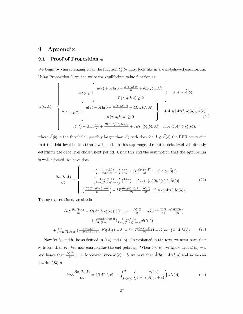
9 Appendix

9.1 Proof of Proposition 4

We begin by characterizing what the function b∗c(b) must look like in a well-behaved equilibrium.

Using Proposition 3, we can write the equilibrium value function as:

vc(b,A) =

⎧⎪⎪⎪⎪⎪⎪⎪⎪⎪⎪⎪⎪⎪⎪⎨⎪⎪⎪⎪⎪⎪⎪⎪⎪⎪⎪⎪⎪⎪⎩

max(τ,g)

⎧⎪⎪⎨⎪⎪⎩u(τ) +A ln g + B(τ,g,b,b)

n + δEvc(b,A0)

: B(τ, g, b, b) ≥ 0

⎫⎪⎪⎬⎪⎪⎭ if A > bA(b)

max(τ,g,b0)

⎧⎪⎪⎨⎪⎪⎩u(τ) +A ln g + B(τ,g,b0,b)

n + δEvc(b0, A0)

: B(τ, g, b0, b) ≥ 0

⎫⎪⎪⎬⎪⎪⎭ if A ∈ [A∗(b, b∗c(b)), bA(b)]u(τ∗) +A ln qA

p +B(τ∗, qAp ,b∗c(b),b)

n + δEvc(b∗c(b), A

0) if A < A∗(b, b∗c(b)),

(21)

where bA(b) is the threshold (possibly larger than A) such that for A ≥ bA(b) the BBR constraintthat the debt level be less than b will bind. In this top range, the initial debt level will directly

determine the debt level chosen next period. Using this and the assumption that the equilibrium

is well-behaved, we have that

∂vc(b,A)

∂b=

⎧⎪⎪⎪⎪⎪⎪⎨⎪⎪⎪⎪⎪⎪⎩−³

1−τb(A)1−τb(A)(1+ε)

´ ¡ρn

¢+ δE ∂vc(b,A

0)∂b if A > bA(b)

−³

1−τc(b,A)1−τc(b,A)(1+ε)

´ ¡1+ρn

¢if A ∈ [A∗(b, b∗c(b)), bA(b)]³

db∗c(b)/db−(1+ρ)n

´+ δE

∂vc(b∗c(b),A

0)∂b

db∗c(b)db if A < A∗(b, b∗c(b)).

(22)

Taking expectations, we obtain

−δnE ∂vc(b,A)∂b = G(A∗(b, b∗c(b)))δ[1 + ρ− db∗c(b)

db − nδE∂vc(b

∗c(b),A)∂b

db∗c(b)db ]

+Rmin{A, bA(b)}A∗(b,b∗c)

( 1−τc(b,A)1−τc(b,A)(1+ε) )dG(A)

+R Amin{A, bA(b)}( 1−τb(A)

1−τb(A)(1+ε) )dG(A)(1− δ)− δ2nE ∂vc(b,A)∂b (1−G(min{A, bA(b)})). (23)

Now let b0 and b1 be as defined in (14) and (15). As explained in the text, we must have that

b0 is less than b1. We now characterize the end point b0. When b < b0, we know that b∗c(b) = b

and hence thatdb∗c(b)db = 1. Moreover, since b∗c(b) = b, we have that bA(b) = A∗(b, b) and so we can

rewrite (23) as:

−δnE∂vc(b,A)

∂b= G(A∗(b, b)) +

Z A

A∗(b,b)

µ1− τb(A)

1− τb(A)(1 + ε)

¶dG(A). (24)

37

Since b0

q + δEvc(b0, A0) is constant on the interval [b0, b1], the right hand derivative of the value

function at b0 and the left hand derivative at b1 must be 1/q. Since the expected value function is

differentiable, then, we must have that at b0 the left hand side derivative (which is given by (24))

is 1/q implying that

G(A∗(b0, b0)) +

Z A

A∗(b0,b0)

µ1− τb0(A)

1− τb0(A)(1 + ε)

¶dG(A) =

n

q.

This is (18).

The next step is to characterize b∗c(b) on the interval [b0, b1]. Ifbq + δEvc(b,A

0) is constant on

the interval [b0, b1] we must have that

−δnE∂vc(b,A)

∂b=

n

q, (25)

for any b ∈ [b0, b1]. Since E ∂vc(b,A)∂b is a function of b∗c(b) and its derivative, (25) implies a

differential equation that needs to be satisfied by b∗c(b) along with the initial condition b∗c(b0) = b0.

Using (23), we can show that this condition requires that b∗c(b) in [b0, b1] is equal to a function

f (b) that solves the differential equation:

nq = G(A∗(b, f(b)))

h1− df(b)

db δ³1− n

q

´i+(nq )(1− δ)G(A∗(b, b))− (nq )G(A∗(b, f(b))) +

R AA∗(b,b)

³1−τb(A)

1−τb(A)(1+ε)

´dG(A)(1− δ) + δ nq ,

with the initial condition f(b0) = b0. This is (19). Note that if this condition is satisfied, then

any point in [b0, b] would be a legitimate choice for b∗c(b) when b ∈ [b0, b1]. We are therefore free

to choose b∗c(b) as we like - in particular, b∗c(b) = f(b). By Theorem 20 in Braun (1992) (p.77),

f(b) is uniquely defined on [b0, b].

The final step is to pin down the end point of the interval b1. Because b∗c(b) is non decreasing

and bounded in [b0, b1], it must be constant and equal to f(b1) for debt levels b larger than b1.

Using (23) and the fact thatdb∗c(b)db = 0 for b greater than b1 we have that:

−δnE∂vc(b,A)

∂b=

G(A∗(b, b∗c(b))) +Rmin{A, bA(b)}A∗(b,b∗c(b))

³1−τc(b,A)

1−τc(b,A)(1+ε)

´dG(A)

+R Amin{A, bA(b)}

³1−τb(A)

1−τb(A)(1+ε)

´dG(A)(1− δ)

1− δ(1−G(min{A, bA(b)})) . (26)

for b greater than b1. The same logic used to pin down b0 can now be used for b1: at b1 we need

the right hand side derivative (given by (26)) equal to 1/q. This implies that b1 must satisfy:

n

q(1−δ) = n

q(1−δ)G(A∗(b1, b1))−

µn

q− 1¶G(A∗(b1, f(b1)))+

Z A

A∗(b1,b1)

µ1− τb1(A)

1− τb1(A)(1 + ε)

¶dG(A)(1−δ).

38

This is (20).

We now have a full characterization of the b∗c(b) function in a well-behaved equilibrium. Notice

that for a given b∗c(b) function, (13) is a contraction with a unique fixed-point. Thus, since b∗c(b)

is uniquely defined, there exists a unique well-behaved equilibrium. ¥


Note first from (13) and (17) that b0c(b0, A) = b0 for all A so that b0 is a steady state. The key

step is therefore to show that the equilibrium level of debt must converge down to the level b0.

Let bb ∈ [b∗, b) denote the debt level that is prevailing when the BBR is imposed. Since the BBRimplies that debt can never go up, what we need to show is that for any b ∈ (b0,bb] the probabilitythat debt remains at b goes to zero as t goes to infinity.

Given an initial debt level b ∈ [b0,bb], let Hm(b, b0) denote the probability that in m periods

debt will be less than b0 ∈ [b0, b] given the equilibrium debt policy function b0c(b0, A). Suppose

that we could show that for any initial b ∈ (b0,bb] there exists an ε > 0 and an integer m such that

Hm(b, b∗c(b)) exceeds ε. Then we could conclude that for any b ∈ (b0,bb] the probability that debtremains at b goes to zero as t goes to infinity. To prove this, choose any b ∈ (b0,bb] and let ς > 0.Then we need to show that there exists some tς such that the probability that debt is equal to b

after tς periods is less than ς. But we know that after t ·m periods the probability that debt will

equal b will be less than [1−Hm(b, b∗c(b))]t < (1− ε)t. By choosing tς such that (1− ε)tς/m ≤ ς

we obtain the desired result.

We now establish:

Claim 1: For any b ∈ (b0,bb], there exists an ε > 0 and an integer m such that Hm(b, b∗c(b)) ≥ ε.

Proof: For any b ∈ [b0,bb] and A ∈ [A,A] define the sequence hφm(b,A)i∞m=1 inductively as follows:φ0(b,A) = b and φm+1(b,A) = b0c(φm(b,A), A). Thus, φm(b,A) is the equilibrium level of debt if

the debt level were b at time 0 and the shock was A in periods 1 through m.

Recall that, by assumption, there exists some positive constant ξ > 0, such that for any pair

of realizations satisfying A < A0, the difference G(A0)−G(A) is at least as big as ξ(A0−A). This

implies that for any b ∈ [b0,bb], Hm(b, φm(b,A+λ))−Hm(b, φm(b,A)) ≥ ξmλm for all λ such that

0 < λ < A−A. To see this, let A = (A1, A2, ..., Ak, ...) be a countable vector of shocks such that

Aj ∈ [A,A+λ] for all j = 1, ...,∞, and for allm letAm = (A1, A2, ..., Am) be the list of the firstm

elements. Define also the sequence hφm(b,Am)i∞m=1 inductively as follows: φ1(b,A1) = b0c(b,A1)

39

and φk+1(b,Ak+1) = b0c(φk(b,A

k), Ak+1). Clearly φ1(b,A1) ∈ (φ1(b,A), φ1(b,A+ λ)). Assume

that φk(b,Ak) ∈ (φk(b,A), φk(b,A+ λ)), then, since b0c(b,A) is increasing in b and A:

φk+1(b,Ak+1) ∈ (b0c(φk(b,A), Ak+1), b

0c(φk(b,A+ λ), Ak+1)

⊂ (b0c(φk(b,A), A), b0c(φk(b,A+ λ), A+ λ)

= (φk+1(b,A), φk+1(b,A+ λ))

It follows that φk+1(b,Ak+1) ∈ (φk+1(b,A), φk+1(b,A+ λ)). This implies that after m periods, if

the initial state is b and if there are m sequential shocks Aj ∈ [A,A+ λ], then debt will certainly

be in (φm(b,A), φm(b,A+ λ)). The probability that after m periods, if the initial state is b, debt

is in (φm(b,A), φm(b,A+ λ)) must therefore be larger than the probability of m sequential shocks

Aj ∈ [A,A+ λ]. This probability is at least (ξλ)m .

Given this, to prove the Claim it suffices to show that there exists an integer m such that

A∗(φm(b,A), b∗c(b)) > A. If this is the case by continuity there is a λm(b) > 0 small enough such

that A∗(φm(b,A+ λm(b)), b∗c(b)) > A. It then follows that

Hm(b, b∗c(b)) =

Zz

H1(z, b∗c(b))dHm−1(b, z)

≥Z φm(b,A+λm(b))

φm(b,A)

H1(z, b∗c(b))dHm−1(b, z)

≥ H1(φm(b,A+ λm(b)), b∗c(b))

£Hm−1(b, φm−1(b,A+ λm(b)))−Hm−1(b, φm−1(b,A))

¤≥ H1(φm(b,A+ λm(b)), b

∗c(b)) (ξλm(b))

m−1 > 0.

The third inequality follows from the facts that H1(b, b0) is non-increasing in b and φm(b,A +

λm(b)) ≥ φm(b,A).

It remains to show that there exists an integer m such that A∗(φm(b,A), b∗c(b)) > A. Suppose,

to the contrary, that for all m we have that A∗(φm(b,A), b∗c(b)) ≤ A. To simplify notation, let

φm = φm(b,A) for all m. The BBR implies that for all m, φm−1 ≥ φm. We can therefore assume

without loss of generality that the sequence hφmi converges to some finite limit φ∞ ≥ b0. Since

A∗(φm, b∗c(b)) ≤ A and φm ≤ b, we know that G(A∗(φm, b

∗c(φm))) = 0. Thus from (23) we have

that for all m

−δnE∂vc(φm, A)

∂b=

Rmin{A, bA(φm)}A

( 1−τc(φm,A)1−τc(φm,A)(1+ε))dG(A) +

R Amin{A, bA(φm)}( 1−τφm (A)

1−τφm (A)(1+ε))dG(A)(1− δ)

1− δ(1−G(min{A, bA(φm)}) .

40

But we know that it must be the case that

τc(φm, A)

1− τc(φm, A)(1 + ε)≥ −δnE∂vc(φm+1, A)

∂b

where the inequality is strict if the BBR is binding. This means that

τc(φm, A)

1− τc(φm, A)(1 + ε)≥Rmin{A, bA(φm)}A

( 1−τc(φm+1,A)1−τc(φm+1,A)(1+ε)

)dG(A) +R Amin{A, bA(φm)}( 1−τφm (A)

1−τφm (A)(1+ε))dG(A)(1− δ)

1− δ(1−G(min{A, bA(φm)})where the inequality is strict if the BBR is binding. Note however that if φm+1 is sufficiently close

to φm then since τc(b,A) and τb(A) are increasing in A and

1− δ(1−G(min{A, bA(φm)})) < 1,the right hand side must be strictly larger than the left hand side, a contradiction. We conclude

therefore that for m sufficiently large A∗(φm(b,A), b∗c(b)) > A, which yields the result. ¥

The description of what the policies would be at the steady state debt level b0 follows the

characterization following Proposition 3. ¥


We first show that the average primary surplus at the steady state debt level b0 is less than

the average primary surplus in the long run in the unconstrained equilibrium. The primary

surplus is the difference between tax revenues and spending on the public good and pork. In

the unconstrained equilibrium, using the budget constraint, we may write this as PS(b,A) =

(1 + ρ)b − b0(b,A). Let EPS(b) =RPS(b,A)dG(A). Let H(b, b0) be the transition function

implied by the unconstrained equilibrium; that is, the probability that in the next period the

initial level of debt will be less than or equal to b0 ∈ [b∗, b) if the current level is b. Let ψ(b) denote

the long run equilibrium debt distribution. This satisfies the condition that

ψ(b0) =

Zb

H(b, b0)dψ(b).

(For the details see Battaglini and Coate (2008)). Then we have that the average primary surplus

in the long run in the unconstrained equilibrium is

bZb∗

EPS(b)dψ(b) = (1 + ρ)E(b)−bZb∗

b0dψ(b0) = ρE(b)

41

From Proposition 5, we know that the average primary surplus in the steady state under a strict

BBR is just ρb0. We also know that b0 < b∗. Thus we have that

bZb∗

EPS(b)dψ(b) = ρE(b) > ρb∗ > ρb0,

as required.

We next show that the average level of pork-barrel spending at the steady state debt level b0

is larger than the average amount of pork-barrel spending in the long run in the unconstrained

equilibrium. By Proposition 5, average pork-barrel spending at the steady state debt level b0 is

given byA∗(b0,b0)Z

A

B(τ∗, g∗(A), b0, b0)dG(A).

Average pork-barrel spending in the long run in the unconstrained equilibrium is

bZb∗

⎧⎪⎨⎪⎩A∗(b,b∗)Z

A

B(τ∗, g∗(A), b∗, b)dG(A)

⎫⎪⎬⎪⎭ dψ(b),

where ψ(b) is the invariant distribution. We have that

bZb∗

⎧⎪⎨⎪⎩A∗(b,b∗)Z

A

B(τ∗, g∗(A), b∗, b)dG(A)

⎫⎪⎬⎪⎭ dψ(b) ≤A∗(b∗,b∗)Z

A

B(τ∗, g∗(A), b∗, b∗)dG(A)

<

A∗(b0,b0)ZA

B(τ∗, g∗(A), b0, b0)dG(A),

where the last inequality follows from the fact that b0 < b∗. ¥

42

Analyzing the Case for a Balanced Budget...

Documents

Transcript of Analyzing the Case for a Balanced Budget...