1

Analyzing and visualizing numerical methods.

Summary: Methods used to determine the roots of complex polynomialfunctions are introduced and discussed. These methods useinitial values (seed values) for the calculation of the roots.Each root appears to be associated with a specific set ofinitial values. These sets show remarkable patterns withgeometric properties that are distributed in thetwo-dimensional plane defined by the real and the imaginaryaxis of the complex numbers and functions under investigation.The article contains a short introduction to the methods usedto find the roots (solutions) of linear equations, thestrategies used to apply them, as well as the algorithms thatdetermine the roots and render the areas that represent thesets of initial values associated with the calculated roots.A large collection of examples is added.

1. Methods for finding the roots of linear equations.

Linear equations are equations of the form: Y = F(X) where thefunction F of X does not contain a factor or an element of thefunction (Y) itself.An example of a linear functions is: Y = 5X2-3sin(X)+7X-3,while Y = 5X2-3sin(Y)+7XY-3 depicts a non-linear function. Inthe remainder of this article we will restrict ourselves tomethods used to find the roots of linear functions. Those rootsare defined by the solutions that satisfy the condition thatF(X) = 0. Easy to use methods are those that use successivesubstitutions and are known as the method of successivesubstitution and the method of Wegstein. The method ofsuccessive substitution works as follows:

Suppose we have to find the (three) roots of the equation

(1)X X3 7 0− + =In the method of successive substitution we use the equation

(1a)Xn Xn+ = +13 7

to find solutions for equation (1). Starting with anappropriate initial value (further referred to as seed value)for Xn, we calculate Xn+1 with equation (1a), and repeat thisprocess. Depending on the chosen seed value this processconverges in many cases to a situation in which this newlycalculated value does not change any more. In that case one

2

root of equation (1) has been found. It is possible to find thesecond root using a different seed value, but this is far fromguaranteed. The general formula for the method of successivesubstitution is shown in equation (2). When the differencebetween Xn+1 and Xn becomes smaller than a predefined value wehave found a root of the function F(Xn).

(2)Xn 1 F(Xn )+ =

However, this method of the successive approximation does notprovide us with all of the possible solutions of the originalequation:

F(X)=0 (3)Wegstein proposed an alternative to the method of successivesubstitution. This variant will generate many more solutionsthan the strict way in which the newly found value Xn+1 isinserted in the equation containing a function of Xn. This moresuccessful method consists of adding a fraction of the valueof X into equation (2). In that case Xn+1 consists of acombination of the previous value of X and the new value ofF(Xn).That combination is achieved with the aid of a relaxationfactor. The new value used to calculate the right hand side ofequation (2) becomes D.Xn + (1-D).Xn+1 . In this case equation(2) is transformed into:

(4)X X F Xn n n+ = + −1 1ρ ρ. ( ). ( )in which D is the relaxation factor. The difficulty in boththe method of successive substitution and Wegstein's method isthe way in which multiple roots can be found. The beauty ofusing the first method is that is has a fast convergence speedand does not have to use the first derivative of the functionwhose roots we are trying to find. The difficulty in applyingthis method consists of having to isolate X from its equationand bringing it to the zero side of the equation. Thisdifficulty is best shown in solving the equation:

X3 - 2 = 0 (4)This equation can be written as:

X = X3 + x - 2 (5),or

X = (2 + 5X - X3)/5 (6)Applying the method of successive substitution, equation (5)quickly diverges, no matter what seed value of X is being used.Equation (6) however generates a solution with an accuracy of5 fractional digits in 4 steps. A similar problem may be

3

encountered with the use of relaxation factors. ApplyingWegstein's method to many equations showed that most solutionscould be produced by applying high relaxation factors.We have investigated a method that consists of a combinationof the method of successive substitution and Wegstein's method.First we add ".X to the equation at the zero side of theequation and divide the newly constructed equation by ". Thevalue of " is either smaller than or equal to -1 or greaterthan or equal to +1. For instance in the equation:

X3 - 5X2 - 7 = 0 (4a)we add ".X to both sides of the equal sign:

X3 - 5X2 + ".X - 7 = ".X (5a)or: X = (X3 - 5X2 + ".X - 7)/" (6a)With the method of successive substitution we now calculatesuccessive values of

(7)Xn X X X+ = − + −13 5 2 7( . ) /α α

Combining this with Wegstein's method the calculating schemethen becomes:

(8)Xn Xn Xn Xn Xn+ = + − − +1 1 3 5 2ρ ρ α α. ( ).( . ) /We will refer to this approach in the remainder of this articleas the modified Wegstein method.A third method is the method of Regula Falsi. This method isalso an iterative method. The new value of X is calculatedusing the two previously calculated values of X. The method canbe formulated as:

(9)Xn Xn F Xn Xn Xn F Xn F Xn+ = − − − − −1 1 1( ).( ) / [ ( ) ( )]or:

(10)Xn Xn F Xn Xn F Xn F Xn F Xn+ = − − − − −1 1 1 1[ . ( ) . ( ) )] / [ ( ) ( )]

The difficulty is that we have to start with two seed values,one for Xn and one for Xn-1. A more efficient approach is offered by the widely usedNewton-Raphson method. In this iterative method the new valuefor X is calculated using the previously calculated value ofX, F(X) and F'(X), the first derivative of F(X).

(11)Xn Xn F Xn F' Xn+ = −1 ( ) / ( )Where the methods of successive substitution and Wegstein arereasonably simple and straightforward, Regula Falsi andNewton-Raphson do respectively need the use of two previouslydetermined (or chosen) values of X and the first derivative ofthe function whose roots we try to determine. The unmodified

4

method of successive substitution is used widely in thecreation of fractals (see Part 1 of this chronicle), howeverwithout trying to find the roots of the equations that definethe fractals. The process of successive substitutions stops inthe generation of fractals as soon as this iteration processstarts to diverge. The author used the methods of Regula Falsiand Newton-Raphson in order to demonstrate the beauty ofpatterns that are created when these methods are applied tofind roots of higher degree polynomial equations. For thatspecific purpose we have focused on determining the roots ofcomplex polynomials, that is polynomials of the form:

anZn+an-1Zn-1+.............a2Z2+a1Z+a0=0 (12)or

(13)a Zmm

m nm

=

=

∑ =0

0

In this case the coefficients of formula(13) are real numbersand Z are complex numbers. In casethe coefficients are also complexnumbers equation (13) is writtenas:

(14)C Zmm

m nm

=

=

∑ =0

0

with coefficients C = a + i.b (aand b are real numbers).

Complex numbers are represented inthe Euclidian two-dimensional spaceas coordinates whose real number isrepresented by the value of the

X-coordinate and whose imaginary number is represented by thevalue of the Y-coordinate. The absolute value of a complex number is its distance to theorigin, being /(X2+Y2). Positive real numbers coincide with itsvalues of the positive X-axis and positive imaginary numberswith the positive Y-axis.Note that the methods of the modified Wegstein, Regula Falsiand Newton-Raphson can be applied to rational as well ascomplex numbers.

5

2. Strategy of determining the roots.

The strategy used to calculate the roots of equations with theaid of the modified Wegstein approach consist of firstcalculating one root with the appropriate values of D and ".The original equation is then divided by (Z-Z1) where Z1 is thefirst found root. This results in a new equation:

Fnew(Z) = F(Z)/(Z-Z1) = 0 (15)In this way we can apply modified Wegstein for finding root nfrom

(16)Fnew Z) F Z) Z Zkk

k n( ( / ( )= −

=

=∏1

For each Fnew(Z) = 0 the in formula (16) annotated divisionprocess will change.Each set of coefficients for the equations that are a degreelower than the original one can be calculated from the previousone in the following way:

Establish the value of the root Z from the lastly created equation. Determine the newdegree of the equation by lowering the previous degree by one. This results in the newdegree k.BEGINFOR i = k TO 1 DO

(17)C Z Z Cik i n

n

n k i

i n−− +

=

= −

+= + ∑11

0.

END The coefficients of the equation are denoted by the symbols .Cn

The roots of the thus created equations can be calculated withthe modified Wegstein method. For each equation the appropriatevalues of " and D have to be established. The process ofcreating new equations can stop as soon as the degree of themost recently created equation is 2. Calculation of the last2 roots is straightforward.Since we are using previously calculated roots for determiningthe coefficients of an equation with a lower degree, errorsintroduced in these roots will be propagated to the newlycalculated coefficients. For each set of coefficients the errorfunction will be represented by the formula:

6

(18)Ε ( ) .C Cik i n

n

n k i

i n−− +

=

= −

+= + ∑11

1δ δ

where denotes the error function for the calculatedΕ ( )Ci−1coefficient and * denotes the difference between the previouslycalculated root and the actual value of this root. The

dominating factor in the error function consists of . Allδ( )Ci n+

the other factors can be neglected since they contain powersof the small value *. It may be useful to calculate the rootof the newly created equation and use this root as seed valuein the original equation (14).However one should not be surprised that modified Wegstein willconverge to an earlier calculated root of this equation.Another way of calculating the roots with modified Wegsteinconsists of creating a new equation by dividing the originalequation by the product of (Z-Z1).(Z-Z2)....(Z-Zn) wheren=1,2,3..... are the already found roots.The roots can then be determined through the followingiterative modified Wegstein procedure:

Determine seed values for Z. Calculate:

(19)Z Z F Z Z Z Zn n nn

n k

+=

=

= + − − +∏11

1ρ ρ α α. {( ).[ ( ) / ( )] . } /

Repeat until the absolute value of (Zn+1-Zn) becomes smaller than a predeterminedaccuracy.

This second procedure is more complicated than the previouslydescribed one because it becomes more difficult to determinethe values of " and D to make the iterative process converge.However, there are also losses in significance here since weuse the earlier calculated roots to determine a next one. Thoseroots are as accurate as the specified accuracy.

The strategy applied to calculate the roots of an nth-degreepolynomial equation is straightforward. In a rectangular areain the complex two-dimensional plane defined by its left-bottomand right-upper coordinates, seed values for Regula Falsi andNewton-Raphson are determined. For a fixed real value weincrease the imaginary value with a specified value (say .01times the difference between the highest and the lowest value

7

of the imaginary or vertical axis). When the lowest value hasbeen reached, the value of the real part of the seed value isincreased with a specified value and the process of determiningincremental values along the imaginary axis starting with thehighest is resumed. These seed values are directly applied forthe Newton-Raphson method. Since we need two seed values forRegula Falsi another value (Zn-1) which differs slightly fromthe seed value (Zn) obtained with the above mentioned scheme.As soon as a root has been found it is placed in a list. Theroots obtained with this process are then compared with thosein the list and added to this list if they are not yet placedin this list. When the maximum number of roots, determined bythe degree of the equation, has been found the process stops.The Newton-Raphson method works well without problems. RegulaFalsi poses some problems due to the fact that a loss ofsignificancy in the result of the calculations may occur. Thedivisor in the formula of Regula Falsi tends to become verysmall when using certain seed values. It is therefore necessaryin this method to substitute the found roots in the equationand determine whether or not the result of this substitutionis close enough to zero. If this is not the case this resultis rejected as a viable root of the equation.

3. Visualizing the association between seed values and roots.

With the Newton-Raphson method the seed values used todetermine one particular root of equation (14) appear to beclustered in specific parts of any rectangular area in the two-dimensional plane defined by the X-axis (real numbers) and Y-axis (imaginary numbers) that contain the complex numbers ofthe roots of said equation. We will now associate those rootswith a colour and repeat the root-finding process as describedin the previous chapter. Since we are working with a displayscreen that contains 640 horizontal pixels and 480 verticalpixels we divide the chosen length of the X-axis by 640 and theY-axis by 480. These numbers determine the increments alongboth axis which are used to specify the seed values and areassociated with the pixels of the screen. When a root is foundthe pixel is coloured in accordance with the colour associatedto that specific root. If we don't find a root with a set ofseed values the pixel will be coloured black. What happens isthat either we are not continuing the iterative procedure longenough or difficulties are encountered due to a loss of

8

significance in the calculation methods. This is especially thecase when dealing with very small numbers. The result of thisprocess is a screen that contains as many colours as the degreeof the equation of which we are trying to find the roots plusthe extra colour black in case not a single root can be found.In the examples of the next chapters one notices large areasof colours that are fringed with specific smaller patterns(leafs) in which all colours reappear. The larger areas neverborder directly to each other. These fringes of patterns actas barriers and exhibit the same characteristics when viewingon smaller scales as the ones that are generated within therectangular areas. We distinguish here between higher and lowerorder leafs. Any leaf that is part of this fringe (barrier) issaid to be of a lower order than the leaf that is bounded(surrounded) by such a barrier. Regula Falsi displays a similar pattern be it that the seedvalues which are used to find the roots occupy a much largerpart of the screen. The characteristics of the colour patternsare also definitely different from those that are obtained withNewton-Raphson. To avoid the iterative processes fromcollapsing due to iterations that could diverge, wediscontinued the iterative processes after certain (large)values of the calculated function F(Z) were generated. Thesebrake-off values are named blowouts in our processes.

9

4. Examples.

a. Z15-1 =0

For equation Z15-1=0 we find the following 15 roots with programROOTNR.BAS or ROOTRF.BAS with a predefined accuracy of .0001 and anallowed number of iteration steps of 50. The accuracy is heredefined as an absolute value. The absolute value of the accuracyshould be less than a specified small number, here .0001. Theabsolute value of the accuracy is defined as the calculated Znminus the previously calculated value Zn-1. For small numbers weterminate the iteration process if the relative value of theaccuracy is smaller than .0001. The roots of this equation (calculated with ROOTNR.BAS andROOTRF.BAS) are: Root 1: -.8090169943749569+.5877852522924623*iRoot 2: -.9781476007337959+.2079116908177389*iRoot 3: -.9781476007338028-.2079116908177727*iRoot 4: -.8090169943750308-.5877852522924524*iRoot 5: -.5000000000000118+.8660254037844382*iRoot 6: -.4999999999999881-.8660254037844456*iRoot 7: -.1045284632614425+.9945218953630895*iRoot 8: -.1045284632675011-.9945218953682529*iRoot 9: .3090169943749355+.9510565162952112*i Root10: .3090169943749613-.9510565162952028*iRoot11: .9135454576426738-.4067366430758145*iRoot12: .9135454576413630+.4067366430771705*i Root13: 1.0000000000000000+ 2.6337851253D-14*i Root14: .6691306063588788-.7431448254773757*i Root15: .6691306063588582+.7431448254773941*i

The pictures of the seed values are shown in the next three pagesand were created with program GRAPHNR.BAS, a program thatcalculates the roots of a complex polynomial function with theNewton-Raphson method. The little white squares in the first twopictures indicate the areas of the next picture. The processes usedan accuracy of .0001, and a maximum of 200 iteration steps. Noblowout value was defined in this procedure. The defined boundariesof the pictures are respectively defined by the corner valuesdefined by the complex numbers x1+y1.i and x2+y2.i (the frame(window) values) of the rectangular areas used to find the roots.The values x1,y1,x2,y2 are respectively for picture a1:-1,-1,1,1;for picture a2: .6,.4,.8,.6; and for picture a3: .76,.44,.8,.48.A fourth picture a4 shows the seed values and its associated rootswhen using the Regula Falsi method. The frame (window) values arehere the same as in picture a1. The picture was created withprogram GRAPHRF.BAS, a program that calculates the roots of acomplex function with the Regula Falsi method.

10

11

12

b. Z9-0.25*Z6-0.75*Z-1=0

The roots of this equation (calculated with ROOTNR.BAS) are:

Root 1: -.5765285440398880+0.8297399226570532*iRoot 2: -.8426374259810665-0.2776090046342414*i Root 3: -.5765285436531420-0.8297399226783863*iRoot 4: .083395869263670-1.0180125870967600*i Root 5: -.8426374184313042+0.2776089929328531*iRoot 6: .7886269646291705-0.6842198841400152*i Root 7: 1.0942863011577480+4.456371336457D-21*i Root 8: .7886269646291506+0.6842198841400370*i Root 9: .0833958692636420+1.0180125870967600*i

The picture b1 generated with Newton-Raphson is defined through thefollowing properties:frame (window) coordinates:-1,-1,1,1accuracy: .0001max. number of iterations: 50blowout factor: 25used program: GRAPHNR.BAS

13

c. Z9+Z8+Z7+Z6+Z5+Z4+Z3+Z2+Z-9=0 The roots of this equation (calculated with ROOTNR.BAS and checkedwith ROOTFR.BAS) are:Root 1: 0.8767318053938815+0.8813721268235023*iRoot 2: 0.1363853102203647+1.3049529205205450*iRoot 3: -1.2887565879577400+0.4476823059014147*iRoot 4: 0.9999999999228558-9.693678035294D-11*i Root 5: 0.8767318053942852-0.8813721268234147*i Root 6: -0.7243605276648716-1.1369753430223000*i Root 7: -0.7243605281367599+1.1369753433593070*iRoot 8: 0.1363853103183150-1.3049529203976810*i Root 9: -1.2887565879536050-0.4476823058987583*i

The pictures c1 and c2 generated with Newton-Raphson is definedthrough the following properties:frame coordinates: -1,-1,1,1 (c1) and -.22,.18, -.18,.22 (c2)accuracy: .0001max. number of iterations: 100blowout factor: 25used program: GRAPHNR.BASPicture c3 is generated with Regula Falsi. frame (window) coordinates: -3,-3,3,3; accuracy: .000001 max. number of iterations: 50. program used: GRAPHRF.BAS

14

15

d. Z9-Z8+Z7-Z6+Z5-Z4+Z3-Z2+Z-9=0The roots of this equation (calculated with ROOTNR.BAS and checkedwith ROOTRF.BAS) are:Root 1: -.8090169943749472+.5877852522924731*iRoot 2: .3090169943749453+.9510565162951531*i Root 3: .8090169944067819-.5877852522880759*iRoot 4: -.3090169943749475+.9510565162951536*i Root 5: .8090169943749497+.5877852522924707*i Root 6: 1.0000000000000000+.210367301594D-19*i Root 7: -.3090169943750117-.9510565162951868*i Root 8: .3090169943749474-.9510565162951535*i Root 9: -.8090169943748735-.5877852522923932*i

The picture d1 and d2 generated with program GRAPHNR.BAS (Newton-Raphson) are defined through the following properties:frame coordinates: -1,-1,1,1 (d1) and -.65,-.65,-.55,-.55 (d2)accuracy: .0005max. number of iterations: 100Picture d3 was generated with GRAPHRF.BAS (Regula Falsi) and hasthe following properties:frame (window) coordinates: -1,-1,1,1accuracy: .000001max. number of iterations: 100

16

17

e. Z9-.95*Z8-.9*Z7-.85*Z6-.8*Z5+1.05*Z4+1.1*Z3+1.2*Z2+1.25*Z-1=0The roots of this equation (calculated with ROOTNR.BAS) are:Root 1: 1.167338901915678-.483216600656D-18*i Root 2: .474812922934232-.942126622561D-14*i Root 3: -.966489433080152+.2925827948742883*i Root 4: -.966489433116265-.2925827951932694*i Root 5: -.391305685033525+.9377739877101967*i Root 6: -.391305685029391-.9377739877048538*i Root 7: 1.672153464877153+.547173586703D-30*i Root 8: .175642467283891+.9969502735377460*i Root 9: .175642467283891-.9969502735377460*i The pictures e1 through e4 are generated with GRAPHNR.BAS and aredefined through the following properties:frame (window) coordinates: -1,-1,1,1 (e1); -1,.6,-.8,.8 (e2); -.945, .715,-.935,.725 (e3); and -.9371,.7242,-.9369,.7274 (e4)accuracy: .0001max. number of iterations: 50Picture e5 was generated with GRAPHRF.BAS and has the followingproperties:frame (window) coordinates: -1,-1,1,1accuracy: .000001max. number of iterations: 50

18

19

20

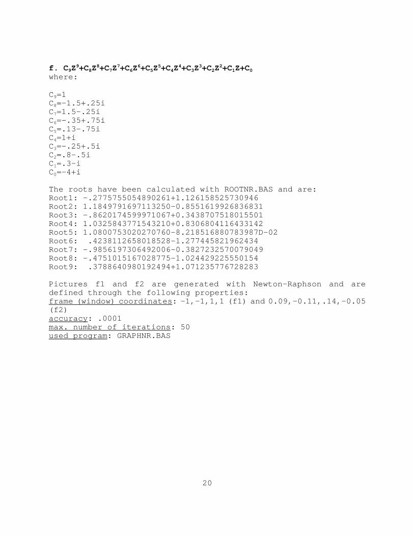
f. C9Z9+C8Z

8+C7Z7+C6Z

6+C5Z5+C4Z

4+C3Z3+C2Z

2+C1Z+C0where:

C9=1C8=-1.5+.25iC7=1.5-.25iC6=-.35+.75iC5=.13-.75iC4=1+iC3=-.25+.5iC2=.8-.5iC1=.3-iC0=-4+i

The roots have been calculated with ROOTNR.BAS and are:Root1: -.2775755054890261+1.126158525730946 Root2: 1.1849791697113250-0.8551619926836831 Root3: -.8620174599971067+0.3438707518015501 Root4: 1.0325843771543210+0.8306804116433142 Root5: 1.0800753020270760-8.218516880783987D-02 Root6: .4238112658018528-1.277445821962434 Root7: -.9856197306492006-0.3827232570079049 Root8: -.4751015167028775-1.024429225550154 Root9: .3788640980192494+1.071235776728283 Pictures f1 and f2 are generated with Newton-Raphson and aredefined through the following properties:frame (window) coordinates: -1,-1,1,1 (f1) and 0.09,-0.11,.14,-0.05(f2)accuracy: .0001max. number of iterations: 50used program: GRAPHNR.BAS

21