2007 ACEEE Summer Study on Energy Efficiency in Industry T

Analyzing and Optimizing the Environmental Performance of Supply Chains

Kumar Venkat, Surya Technologies, Inc. (www.suryatech.com)

ABSTRACT

Supply chains are becoming increasingly vulnerable to energy prices and greenhouse gas emission constraints. Supply chains now span long distances and require significant use of fossil fuels and carbon-dioxide emissions to transport goods to consumers. At the same time, techniques such as lean manufacturing are keeping inventory levels low and require frequent replenishment throughout the supply chain – which can further add to the energy use and emissions, depending on the product. The total energy use and emissions in supply chains depend on transport modes, frequency and size of deliveries, and inventory levels.

We present a methodology for formulating and analyzing this problem at the system level, based on modeling and simulation techniques. Our analysis focuses on transportation and storage along supply chains, both of which consume energy and produce carbon-dioxide emissions. Using a software package that incorporates the methodology presented in this paper, we study the energy use, emissions and cost in selected supply chains from various industry sectors. For products requiring temperature control, such as many food products, we show that there is typically a tradeoff between energy efficiency in transportation and energy efficiency in storage.

Our results suggest that the system-level quantitative method presented in this paper can reveal significant opportunities for improving the energy and emissions footprints of supply chains. As the need for environmental performance increases in the coming years, such quantitative approaches will become increasingly important for supporting management decisions. Introduction

Environmental sustainability is fast becoming the watchword in both industry and

government. Concerns about issues such as global warming appear to be widespread and no longer the exclusive domain of environmental activists. There is some evidence that we may be close to a tipping point in terms of awareness and support for environmental protection and performance. Large corporations – including Wal-Mart, Hewlett-Packard, Nike, and many others (GreenBiz 2006a; GreenBiz 2006b; Holmes 2006) – are beginning to make strong environmental commitments. In the U.S., state governments are now taking a major stand on sustainability. California’s landmark legislation to cap greenhouse gas emissions (Zapler 2006) is being followed by plans to implement a cap-and-trade system by a coalition of five Western states (Milstein 2007).

The emergence of sustainable business depends in part on quantitative tools and methods for analyzing and optimizing the environmental performance of complex systems and networks. Our motivation in this work is to address this need using modeling, simulation and analysis techniques. Among the many sustainability problems in industry that can benefit from quantitative solutions, the analysis and optimization of supply chains stands out as one of the

significant ones. Supply chains are ubiquitous and form the foundation of global commerce. Sustainability of business is a function of the sustainability of the underlying supply chains.

Global supply chains now span long distances and require significant use of fossil fuels to deliver goods to consumers (Venkat 2003). A well-known effect of this is the so-called “food miles”, which refer to the long distances that food products travel to reach consumers. For example, fresh fruits and vegetables travel over 1500 miles on average within the U.S., and over half of the energy consumption associated with food production is related to transportation (Pirog et al. 2001). In addition, the low inventory levels due to the adoption of lean principles require frequent replenishment of goods throughout a supply chain. This can further increase the energy use and emissions, depending on the product (Venkat and Wakeland 2006).

The resource intensive nature of supply-chain networks is highlighted by the fact that freight transport now consumes nearly a quarter of all the petroleum worldwide and produces over 10 percent of the carbon emissions from fossil fuels (Heywood 2006; Socolow and Pacala 2006). Shippers increasingly value speed and reliability and favor transport by truck and airfreight, which are the most energy intensive modes, at the expense of rail and ocean transport (Greene and Schafer 2003).

Supply chains are therefore vulnerable to higher oil prices and limits on greenhouse gas emissions. The purpose of this paper is to describe a method of analyzing, quantifying and improving energy use and emissions in supply-chain networks by taking a system-level view of the problem. We focus here not only on transport links, but also on other elements of supply chains such as storage locations, as well the interaction between them. We quantify the energy used and emissions generated as raw materials and finished goods make their way through supply chain networks. Our results suggest that the system-level quantitative method presented in this paper can reveal significant opportunities for improving the energy and emissions footprints of supply chains.

Objectives and Assumptions

We use the following three metrics to measure the environmental performance of a

supply chain as materials move through transport links and are stored temporarily in storage facilities along the way:

• Energy or fuel consumption due to transport and storage. • Carbon-dioxide (CO2) emissions due to transport and storage. • Financial cost of operating the supply chain, excluding the production steps.

We present a modeling and analysis method that is highly suited for evaluating supply-

chain environmental performance. We then apply this method to analyze selected supply chains from various industry sectors. Our goal is to demonstrate a viable methodology for the analysis and exploration of the solution space, and to extract general insights that can be used to optimize environmental performance.

Although we include production steps in our analysis, we do so at a high level and assume that the production batch sizes are fixed for our purposes. Thus, the variables that we control are directly related to transportation and storage. On transport links where road transport modes are used, we assume for simplicity that full truck load shipments are transported, which is also the most efficient means of using road transport modes. This implies that shipment sizes will

be determined by the capacities of the specific types of trucks used. We also assume in our experiments that non-renewable sources of energy are used in both transport and storage; thus, energy use and CO2 emissions are considered to be highly correlated, although actual emissions per unit energy consumption will vary depending on the specific energy source.

Modeling and Analysis Method

Figure 1 illustrates a generic supply chain consisting of two storage facilities, labeled

“Inventory1” and “Inventory2”, and two transport links labeled “Supply1” and “Supply2”. This may be seen as a prototype for the actual supply chain examples that we will consider in this study.

Figure 1. Generic two-stage supply chain

storagechain wwhere used pin this

availabThe shload sh

= Di/Sithe ith tthe suconsid

where produc

of prodIj(t), Eused pdependlocatio

terms (based o

Inventory2Delivery

Inventory1Supply1 Supply2

We start by formulating a general model for the energy used by transportation and in a supply chain. The total average energy consumed per unit time in operating a supply ith N transport links and M storage locations can be expressed as E = ∑ ETi + ∑ ESj,

ETi is the energy used per unit time in the ith transport link (i = 1…N) and ESj is the energy er unit time in the jth storage location (j = 1…M). We measure energy in gigajoules (GJ) paper. On each of the N transport links, a transport mode TMk is selected from one of K le transport modes, which has the capacity to transport Ck units of the product at a time. ipment size Si on each transport link is limited by Ck, and is equal to Ck when full truck-ipments are used with road transport modes. The shipment frequency (number of shipments per unit time) on each transport link is Fi

, where Di is the demand for the product (number of units of the product per unit time) on ransport link. Di is proportional to the final consumer demand for the product at the end of pply chain, which we assume to be uniformly spaced for the time frame under eration. The average energy consumed per unit time on each transport link is ETi = Di Ki ETMk,

Ki is the distance of the link and ETMk is the average energy used per unit distance and unit t (expressed in units such as GJ/kg-km) by transport mode TMk. The average energy consumed per unit time at each storage location is ESj = Ebj + (Euj/Tj) ∫ Ij(t) dt, where the function Ij(t) represents the inventory level (number uct units) over time, Tj is an appropriate “time period” of the periodic inventory function

bj is a minimum fixed energy used per unit time by the facility, Euj is the additional energy er unit of the product in storage, and the integral is evaluated between 0 and T. Ij(t) s on the sizes and frequencies of both incoming and outgoing shipments at each storage n. The CO2 emissions model closely follows the energy model, with each of the energy ETi or ESj, expressed in GJ per unit time) converted to kilograms (kg) of CO2 per unit time n the specific type of energy or fuel used in each part of the supply chain. The cost model

also uses the same basic structure and computes the cost of operating the supply chain due to energy use as well non-energy costs such as transportation and storage overhead costs, including the cost of inventory.

We use a stock-and-flow representation to implement this model in software, similar to a system dynamics model (Sterman 2000; Venkat and Wakeland 2006). Instead of lengthy continuous-time simulations based on numerical integration, we use a bounded event-driven simulation method to perform the analysis efficiently. A similar method is commonly used in the analysis of digital integrated circuits and known as static analysis (Venkat et al. 1996). It is applicable in this case for simulating the steady-state performance of a system in which discrete events, such as arrival of shipments or production of a batch of goods, occur with predictable periodicity. This modeling and analysis method has been implemented in a new interactive software package known as SEAT (SEAT 2007), which we use in our experiments with supply chain examples.

Experimental Results

We start our experiments with a simulation of the prototype supply chain in Figure 1 as a

system dynamics model (following Venkat and Wakeland 2006), using three possible road transport modes as shown in Table 1. The three different truck types have vastly different capacities and carbon-dioxide emission characteristics, with the heavy-duty truck more than 7 times as efficient as the light truck.

Table 1. Characteristics of road transport modes

Transport Mode Maximum Load (kg) Fuel Type CO2 Emissions (g/ton-km)

Heavy-duty Truck (H) 17300 Diesel 62

Midsize Truck (M) 6000 Diesel 122

Light Truck (L) 700 Gasoline 459 Source: Pirog et al. 2001

For the purpose of our experiment, we assume an arbitrary, but frequent demand for the final product of 350 kg once every five hours. We assume that each of the supply links is 1000 km long and that full-truck direct shipments are used. A key parameter in the model is the minimum order size at each stage, which determines the frequency at which the inventory is replaced. For example, if the order size at the second stage is exactly 350 kg, then an order for this amount would be placed by the second stage as soon as that amount of product was delivered to the customer. If this minimum order size is increased, the average inventory level would increase correspondingly and the frequency of replenishment would decrease.

In the case of a lean supply chain, the minimum order size would be as close to 350 kg as possible so that replenishment orders closely follow the delivery patterns. Moreover, both stages in the supply chain would be tightly synchronized and inventory levels would be very low. Figure 2 shows the total emissions per unit weight of the product as a function of the minimum order size. The energy characteristic will be similar for most non-renewable energy sources and not shown here. As the order size increases past 700 kg, it becomes possible to use midsize trucks instead of light trucks, which produce significantly lower emissions for each unit of product delivered as shown in Table 1. If the order size exceeds 6000 kg, then heavy-duty trucks

become viable and the emissions drop even more. In the absence of cold storage requirements, it is obvious that emissions will reach a minimum at an order size of just over 6000 kg. In reality, the order size can only take on certain discrete values in our experiment because it must match the full capacity of the truck.

Figure 2 also shows the emissions characteristic when cold storage is required at both stages. As the minimum order size increases, inventory levels increase and the average time that products are in storage increases. In this particular model, the cold storage emissions increase linearly with the time spent by the product in storage and the quantity of the product in storage. The second factor captures, in a simplified way, the increased energy use due to additional use of modular refrigeration equipment, as well as other factors such as additional cool-downs (Meier 1996). Thus, a larger minimum order size would lead to increased emissions from storage for each unit of the product, which would have to be balanced against the lower transportation emissions. The cold storage curves – one with nominal emissions of 1 g/kg-hour and the other with 5 g/kg-hour – illustrate this tradeoff. The cold storage curves show that there is likely to be an order size where minimum emissions can be achieved, given the restriction that full-truck shipments must be used. In our example, a midsize truck carrying 6000 kg would provide the best performance for products requiring cold storage.

Figure 2. Carbon dioxide emissions for the supply chain in Figure 1

frfilicSspfoFtr(w

Source: Venkat and Wakeland 2006

We now perform similar analyses, using the SEAT software, on selected supply chains om various industry sectors. In the experiments that follow, the supply-chain network remains xed in each case. We then vary the transport modes and shipment sizes on various transport nks. For each variation, SEAT computes changes to the inventory levels throughout the supply hain. Based on the transport modes, shipment sizes, shipment frequencies and inventory levels, EAT computes the total energy use, carbon-dioxide emissions and cost per unit time for each ecific variation of the supply chain. Nominal capacities, fuel use, and emission characteristics r various transport modes are based on Pirog et al. 2001 and World Resources Institute 2005.

rom an optimization perspective, the dimension of the solution space equals the number of ansport links, if it is assumed that each transport link has a choice of several transport modes ith shipment size either matching the full capacity of the selected transport mode, or chosen

n the following, we limit the degrees of freedom nsport links (or two groups of links) in each case imensional space. delivers windshield wipers to a car manufacturer ated in the figure are for the baseline case. Using he transport modes used on the second and third otors, respectively), keeping the transport modes gy used and carbon-dioxide emissions generated as the transport modes are varied. Since this storage (and we have ignored any other energy y and emissions profiles suggest that using the eled “H” – on both transport links provides the

d wiper supply chain

d from: Jones and Womack 2002

chain: energy and emissions profiles

based on cost or other mode-specific criteria). Iand vary the transport modes on two selected train order to visualize the optimal solution in a 3-d

Our first example is a supply chain that as shown in Figure 3. The transport modes indicthe transport modes listed in Table 1, we vary ttransport links (to Beta Wipers and to Alpha Mfixed at the other links. Figure 4 shows the enerfrom operating this supply chain each day manufactured component does not require coldused in the warehouses in this case), the energlargest-capacity trucks – heavy-duty trucks labbest environmental performance.

Figure 3. Windshiel

Supply-chain description adapte

Figure 4. Windshield wiper supply

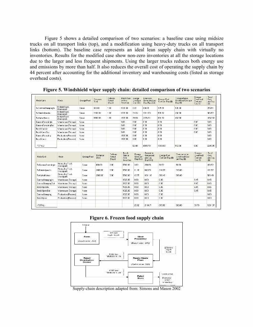
Figure 5 shows a detailed comparison of two scenarios: a baseline case using midsize

trucks on all transport links (top), and a modification using heavy-duty trucks on all transport links (bottom). The baseline case represents an ideal lean supply chain with virtually no inventories. Results for the modified case show non-zero inventories at all the storage locations due to the larger and less frequent shipments. Using the larger trucks reduces both energy use and emissions by more than half. It also reduces the overall cost of operating the supply chain by 44 percent after accounting for the additional inventory and warehousing costs (listed as storage overhead costs).

Figure 5. Windshield wiper supply chain: detailed comparison of two scenarios

Figure 6. Frozen food supply chain

Supply-chain description adapted from: Simons and Mason 2002

Figure 7. Frozen food supply chain: energy and emissions profiles

Figure 8. Frozen food supply chain: detailed comparison of two scenarios

Figure 6 illustrates a frozen food supply chain where the product requires cold storage. The transport modes indicated in the figure are for the baseline case. As seen in Figure 7, the lowest energy use and emissions are achieved when midsize trucks (labeled “M”) are used in both the first and the second transport links in the supply chain, keeping the transport modes fixed in the other links. The product requires cold storage, so there is a clear tradeoff between energy use in transport and energy use in storage. This is demonstrated by the convex shape of the energy and emissions profiles. Even though the most efficient transport mode is the heavy-duty truck (“H”), the optimum solution calls for using midsize trucks in order to keep the inventory levels low enough at each storage location.

Figure 8 shows a detailed comparison of two scenarios: a baseline case (top), and a second case (bottom) which uses larger capacity trucks on all transport links, switching from light trucks to midsize trucks and from midsize trucks to heavy-duty trucks. The average inventory levels rise significantly in the second case. While the second case reduces total energy use and cost, the total emissions actually increase slightly because increased emissions from higher electricity use in storage (due to larger inventories) more than offset the transport emissions saved by switching to larger trucks. This illustrates a potential difficulty in simultaneously optimizing energy, emissions and cost in complex supply chains when different types of energy sources are used in various parts of the supply chain.

Figure 9. Dairy supply chain and energy profile

Supply-chain description adapted from: Food Chain Centre 2005

Figure 9 shows a dairy supply chain. Here, the product requires cold storage and is also produced on a daily schedule that cannot be altered. As indicated in the figure, light trucks are used for daily deliveries to the Newlands Dairy facility, and from there midsize trucks are used to deliver the packaged product to several large customers. The energy profile shows that it is actually less efficient to modify the baseline case and use higher capacity trucks on any of the transport links. This is due to the fact that inventory levels rise as the product is transported less frequently and energy used to maintain the product in cold storage increases far more than any savings obtained from more efficient trucks. The most efficient logistics solution is one that exactly matches the daily production schedule of the product.

Figure 10. Cereal supply chain and energy profile

pttes

Uuifpsmmems

Supply-chain description adapted from: Cereals Industry Forum 2005

The cereal supply chain in Figure 10 requires only a modest level of climate control for roduct storage. The figure indicates the transport modes used in the baseline case. As seen in he energy profile, it much more efficient to switch to heavy-duty trucks because a large part of he energy savings from more efficient transportation can be retained in this case. The additional nergy used to maintain the larger inventories at the Miller and the Biscuit Factory is not ignificant enough.

Figure 11 illustrates a computer manufacturer’s supply chain that produces printers. nlike food products, there are no significant climate control requirements for this product. We se this example to show how an exploration of the solution space can reveal opportunities to mprove overall performance. For the baseline case with transport modes as indicated in the igure, the total energy used per day is 123.4 GJ (which can be seen in the energy profile). If five ercent of the shipments to the Europe Distribution Center use air transport in order to increase ervice levels, then the energy use per day increases to 157.4 GJ. If we then change the transport odes on the road transport links originating from suppliers in Asia, the U.S. and Japan to the ore efficient heavy-duty trucks, the daily energy use decreases to 132.2 GJ. In this hypothetical

xperiment, the supply chain can thus be made more responsive to customer orders with only a odest increase in total energy use by examining the entire supply chain and using energy

avings from one part of the supply chain to speed up the movement of product elsewhere.

Figure 11. Printer supply chain and energy profile

Supply-chain description adapted from: Kopczak and Lee 2001

Discussion and Conclusion

Our experimental results suggest that the system-level quantitative method presented in

this paper can reveal significant opportunities for improving the energy and emissions footprints of supply chains. Based on the experiments, we can make a number of additional observations that can provide some insight into supply-chain environmental performance:

• Transport modes that can deliver larger quantities of a product result in higher inventory

levels, while transport modes that deliver smaller quantities more frequently result in lower inventory levels. Larger inventories generate more emissions and require more energy to maintain, while larger delivery sizes typically have a lower emissions and energy footprint per unit product for transportation. This tradeoff is seen commonly at transport links and associated storage in supply chains for products requiring temperature control, as demonstrated by the experiments in the previous section.

• When warehousing does not require high energy use, such as with manufactured components or certain dry food products, larger shipment sizes and more efficient transport modes can provide better environmental performance. The shipment sizes will, of course, be ultimately constrained by inventory-holding costs.

• When storage is energy-intensive, such as with fresh or frozen food products, optimal shipment sizes and transport modes will vary depending on the product and the supply-chain configuration. Intermediate shipment sizes may work well in many cases.

• Fixed production schedules combined with refrigeration requirements, such as with dairy and some other farm products, typically call for shipment sizes and transport frequencies that are aligned with the production schedule and batch sizes.

• Reducing energy use will reduce CO2 emissions in most cases for non-renewable energy sources, but there may be some exceptions. Due to the tradeoff in energy use between transport and storage, energy use may decrease in transportation while it increases in storage, or vice versa. Depending on the specific energy sources used in the various transport links and storage locations, the total emissions may not decrease as much as total energy use and may even increase slightly in some cases. This may have implications for optimization methods.

• Since emissions can be reduced in most cases by reducing energy use, a more energy-efficient supply chain has a strong potential to contribute to greenhouse gas mitigation efforts. Moreover, if unit energy costs are sufficiently high, then the lower energy costs may be able to offset any increases in non-energy costs (such as inventory-holding costs). Thus, supply-chain environmental performance can translate into cost savings as well. As both energy prices and the market value of carbon offsets or credits continue to increase, a more energy-efficient supply chain will become increasingly cheaper to operate. Supply-chain environmental analysis is a necessary step in evaluating the “goodness” of

supply chains and determining whether further optimization is required. The modeling and analysis method that we have presented in this paper can be used to efficiently analyze specific supply-chain configurations and to compare alternative configurations and options. It can be used to perform rapid “what-if” experiments, such as the ones presented in this paper, and to explore the solution space in search of tradeoffs and more efficient operating conditions. As the need for environmental performance increases in the coming years – driven by public opinion and product marketing on one hand, and higher energy prices and CO2 emission constraints on the other hand – quantitative methods and tools that can directly address environmental performance metrics, such as presented in this paper, will become increasingly important for supporting management decisions. References Cereals Industry Forum. 2005. Smoothing the Flow of Cereals Through the Chain. London, UK:

Cereals Industry Forum. Food Chain Centre. 2005. Building a New Milk Brand. Herts, UK: Food Chain Centre. GreenBiz. 2006a. “Wal-Mart Sustainability Meeting Focuses on Climate Change, Supply

Chain.” GreenBiz.com. July 17. GreenBiz. 2006b. “HP to Cut Greenhouse Gas Emissions, Increase Energy Efficiency of

Products.” GreenBiz.com. November 9. Greene, D.L., and A. Schafer. 2003. Reducing Greenhouse Gas Emissions from U.S.

Transportation. Arlington, Va.: Pew Center on Global Climate Change. Heywood, J. 2006. “Fueling Our Transportation Future.” Scientific American 295 (3): 60-63. Holmes, S. 2006. “Nike Goes for the Green.” Business Week Online. September 25.

Jones, D.T. and J.P. Womack. 2002. Seeing the Whole: Mapping the Extended Value Stream,

Brookline, Mass.: The Lean Enterprise Institute. Kopczak, L.R. and H.L. Lee. 2001. Hewlett-Packard Company: DeskJet Printer Supply Chain

(A). Boston, Mass.: Harvard Business Online. Meier, A. 1996. Toward More Energy-Efficient Use through Demand-Side Management. Berkeley, Calif.: Berkeley Lab, University of California. Milstein, M. 2007. “Oregon Joins 4 States in Greenhouse Battle.” The Oregonian. February 27. Pirog, R., T. Van Pelt, K. Enshayan, and E. Cook. 2001. Food, Fuel and Freeways: An Iowa

perspective on how far food travels, fuel usage, and greenhouse gas emissions. Ames, Iowa: Leopold Center for Sustainable Agriculture.

[SEAT] Supply-Chain Environmental Analysis Tool, Surya Technologies, Inc. 2007.

www.suryatech.com/ep . Portland, Ore.: Surya Technologies, Inc. Simons, D. and R. Mason. 2002. “Environmental and Transport Supply Chain Evaluation with

Sustainable Value Stream Mapping,” In Proceedings of the 7th Logistics Research Network Conference. Birmingham, UK: Logistics Research Network.

Socolow, R.H., and S.W. Pacala. 2006. “A Plan to Keep Carbon in Check.” Scientific American

295 (3): 50-57. Sterman, J.D. 2000. Business Dynamics: System Thinking and Modeling for a Complex World.

New York, NY: Irwin McGraw-Hill. Venkat, K. 2003. “Global Trade and Climate Change.” GreenBiz.com. December 10. Venkat, K., L. Chen, I. Lin, P. Mistry, and P. Madhani. 1996. “Timing Verification of Dynamic

Circuits.” IEEE Journal of Solid-State Circuits 31 (3): 452-455. Venkat, K., and W. Wakeland. 2006. “Is Lean Necessarily Green?” In Proceedings of the 50th

Annual Meeting of the ISSS. York, UK: International Society for the Systems Sciences. World Resources Institute. 2005. Calculating CO2 Emissions from Mobile Sources (GHG

Protocol Initiative). Washington, DC: World Resources Institute. Zapler, M. 2006. “State Senate OKs Emission Caps.” San Jose Mercury News. August 31.