Analyze Demand Data with SAP Predictive Analysis & SAP ... · PDF fileAnalyze Demand Data with...

Analyze Demand Data with SAPPredictive Analysis & SAPDemand Signal Managementpowered by SAP HANA

A detailed step-by-step how-to guide

2

TABLE OF CONTENTS

INTRODUCTION ......................................................................................................................................... 4BUSINESS USE CASE ............................................................................................................................... 5SCENARIO 1: DATA REPLICATION FROM SAP DSIM TO THE SAP PA .................................................. 6Architectural approach .............................................................................................................................. 6Prerequisites .............................................................................................................................................. 7Data Format ................................................................................................................................................ 7HANA Views ............................................................................................................................................... 8Create Attribute Views ................................................................................................................................. 8Create Analytic Views .................................................................................................................................12Create Calculation Views ............................................................................................................................15Predictive Analysis ...................................................................................................................................18Data Visualization .......................................................................................................................................20Data Preparation .........................................................................................................................................25Data Analysis ..............................................................................................................................................25Result Preview ............................................................................................................................................27Result interpretation ....................................................................................................................................28Result Persistency ......................................................................................................................................38

SCENARIO 2: PREDICTIVE ANALYSIS WITHIN SAP HANA AND DATA VISUALIZATION WITH THESAP PA SOLUTION ...................................................................................................................................39Architectural Approach ............................................................................................................................39Prerequisites .............................................................................................................................................39Data Format ...............................................................................................................................................41HANA Views ..............................................................................................................................................42SQL Script to Call PAL K-Means .................................................................................................................42Create Attribute Views ................................................................................................................................47Create Analytic Views .................................................................................................................................47Create Calculation Views ............................................................................................................................47Predictive Analysis ...................................................................................................................................54Data Visualization .......................................................................................................................................56Result Analysis ...........................................................................................................................................56Result Persistency ......................................................................................................................................59Data Preparation .........................................................................................................................................59

COMPLIANCY............................................................................................................................................59ADDITIONAL LINKS ..................................................................................................................................59

Analyze Demand Data with SAP Predictive Analysis & SAP Demand Signal Management

3

Applies to:

SAP Demand Signal Management (DSiM) version 1.0

Summary:

This document describes the necessary technical steps on how to connect the external real-time predictionengine, SAP Predictive Analysis solution (PA), to SAP Demand Signal Management powered by HANA,to provide predictive analysis capabilities out of the box.The approach is to use HANA views, based on the DSiM data model to extract data from the DSiMrepository and analyze it via PA.This how-to paper will describe the following two scenarios, with architectural overview and step-by-stepguide:

Scenario1: POS data in DSiM will be extracted into PA. Predictive analysis and visualization will bedone within the PA solution.

Scenario 2: Predictive analysis will be done in HANA and only visualized in the PA solution.

AuthorsAmina Bounadja Dr. Yue Chenamina,bounadja@sap,com yue,chen@sap,comSAP Canada Inc. SAP AG

Created: July 2013


4

INTRODUCTIONSAP Demand Signal Management (DSiM) powered by SAP HANA enables companies to upload,harmonize, enrich and analyze large amounts of external demand data in order to improve supply chain,sales, marketing and other business processes. With DSiM, customers can get deeper, faster and moreaccurate insight on what is going on in the market (e.g. competitor information or market share information)and also what happens directly on retailer store level. This enables them to react faster to any changes inend-consumer demand.

More and more companies recognize the value that predictive analytics provide. They are looking forsolutions which seamlessly integrate to the existing system landscape and that leverage complex statisticalmodels as central assets in their operational systems. Besides the existing analytics delivered in DSiMstandard solution, it is essential for DSiM customers to have predictive analytics to help uncover trends,patterns, new and old insights in the demand data in DSiM and react to the changes of the end-consumerdemand in timely manner and in some cases ahead of time.

Examples: Forecasting algorithms can be applied to the historical POS data to calculate

predicted sales data, check the sales trend and take the appropriate actions, tomeet the fixed revenue goals.

Clustering algorithms can be used to segment the different retailer stores intoseveral clusters based on KPIs that were enriched from POS data, to assess thestore performance and to be able to help the manufacturer companies identify andreact to specific problems or situations.

The following chapters will outline a step-by-step approach to perform predictive models on DSiM dataleveraging both, the existing predictive capabilities in HANA using PAL (predictive analysis library) and PA(SAP Predictive Analysis) with R integration. All this by the mean of a real business case as describedbelow.


5

BUSINESS USE CASE

A Key Account Manager, of a manufacturing company, who is responsible for a certain retailer accountworks with SAP Demand Signal Management to closely watch supply chain, sales and marketing activities atthis retailer. In collaboration with the company’s Data Analyst, from the business analysis department, whois responsible for data science, data mining as well as predictive data analysis, he wants to analyze DSiMPOS data at retailer store level.

The Data Analyst suggests performing Demand Signal data segmentation for the selected stores, usingsome sales measurements of POS data. This will help to group stores with similar performance andcategorize them in a way that makes it easier to analyze the different groups. Based on the new insight, thekey account manager will be able to take actions to come up with a dedicated plan that meets the needs ofthe single stores.

The Data Analyst proposes to use the K-Means algorithm for segmentation, also called clustering. Thetechnique is making usage of the following POS sales measurements in DSiM: Sales Revenue, SalesQuantity, Average Inventory, Promotion Count, Out Of Shelf Count and Out Of Stock Count.

This can be achieved by following each of the 2 scenarios described below.


6

SCENARIO 1: DATA REPLICATION FROM SAP DSIM TO THE SAP PA

In the first scenario we illustrate the usage of HANA views to extract and replicate DSiM data to SAPPredictive Analysis (PA) solution, where the analysis and visualization is done.Architectural approach


7

Prerequisites

1. Use SAP Predictive Analysis 1.0.10 or later releases2. R engine installed and configured within PA3. Get yourself familiar with the SAP Predictive Analysis solution. User Guide can be found here:

http://help.sap.com/pa

Data FormatAccording to the previously described business use case, the DSiM data that needs to be extracted to allowthe required store clustering, should look like this:

Note:

1. Only store id, highlighted above, is required. Hence, you can skip or add any other attributes youdesire

2. The measures above are chosen to fit the business use case we set above. Hence, feel free to skipor add any other measure according to your use case

3. The listed views are just a proposal for an alternative to extract this data. In case you already knowhow to do that, you can skip the related chapter.

4. Sales_Records_Count highlighted above is also optional, as it is not part of the sales measurementsfor our business use case. Nevertheless, it might be good to have it to allow us to assess the datavolume handled

Within the following section we will list the necessary HANA views to extract this data and also give somehigh level technical guidance on how to build them.


8

HANA ViewsTo replicate DSiM data into PA, the HANA Views below can be used.Note:

This section is not intended as a general presentation of the HANA Views. The approach to design/createHANA views as described in the following sections is not the unique possible one. It is rather to illustratea simplified approach that we followed to extract and prepare the DSiM data for the use of predictivecapabilities provided in PA & HANA, according to the data format we set above.

Create Attribute Views1. Stock data: The view described below is intended to retrieve all Stock data for a given Data Delivery

Context Provider (CDPA) and for a given product.

a. Open HANA Studio and create an Attribute view. We called it ATTR_VIEW_DSIM_STOCK_DATA

b. In the data foundation section, add the DB tables below Product : /1DD/PPRODUCT Location: /1DD/PLOCATION Stock Propagation DSO: /1DD/ADS1200

as shown below:


9

c. Connect the DB tables above using an inner join as shown below

Hint: You can set different accurate filters on each DB table to limit the data to only the one youwant/need to analyse. For instance, you can restrict data to a given country, region and product. Youcan also filter for a given Data Delivery Context Provider (CDPA) from the DSiM data model

d. Output the columns shown below and set Product and Location, from Stock table, as key attributes

e. Save and activate

2. Sales data: The view described below is intended to retrieve all Sales data for a given Data DeliveryContext Provider (CDPA) and product.

Note: The given Data Delivery Context Provider (CDPA) and product are same as the ones used forstock data explained above in step 1


10

a. Open HANA Studio and create an Attribute view. We called it ATTR_VIEW_DSIM_SALES_DATA

b. In the data foundation section add the DB tables below Product : /1DD/PPRODUCT Location: /1DD/PLOCATION Sales Propagation DSO: /1DD/ADS1100

as shown below:

c. Connect the DB tables above using an inner join as shown below


11

Hint: You can set different accurate filters on each DB table to limit the data to the one youwant/need to analyse. For instance, you can restrict data to a given country, region and product. Youcan also filter for a given Data Delivery Context Provider (CDPA) from the DSiM data model

d. Output the columns shown below, where “Sales_Type” is hidden, and set Product and Location,from Sales table, as key attributes

e. To highlight the sales records done within a promotion, you can create the calculated column“Promotion”, as shown below, where “Sales_Type” is the field /1DD/S_SALGRP from SalesPropagation DSO (DB table/1DD/ADS1100):

Note: Based on the formula above, sales records with promotion field equal to 1 are the ones thatbelong to a promotion.

f. Save and activate


12

Create Analytic ViewsThe idea here is to build one analytical view for each attribute view to combine sales and stock data and toadd the product and location attributes.

Details below:

1. Stock data: we called it ANAL_VIEW_DSIM_STOCK_DATA and it is designed as shown below:


13


14

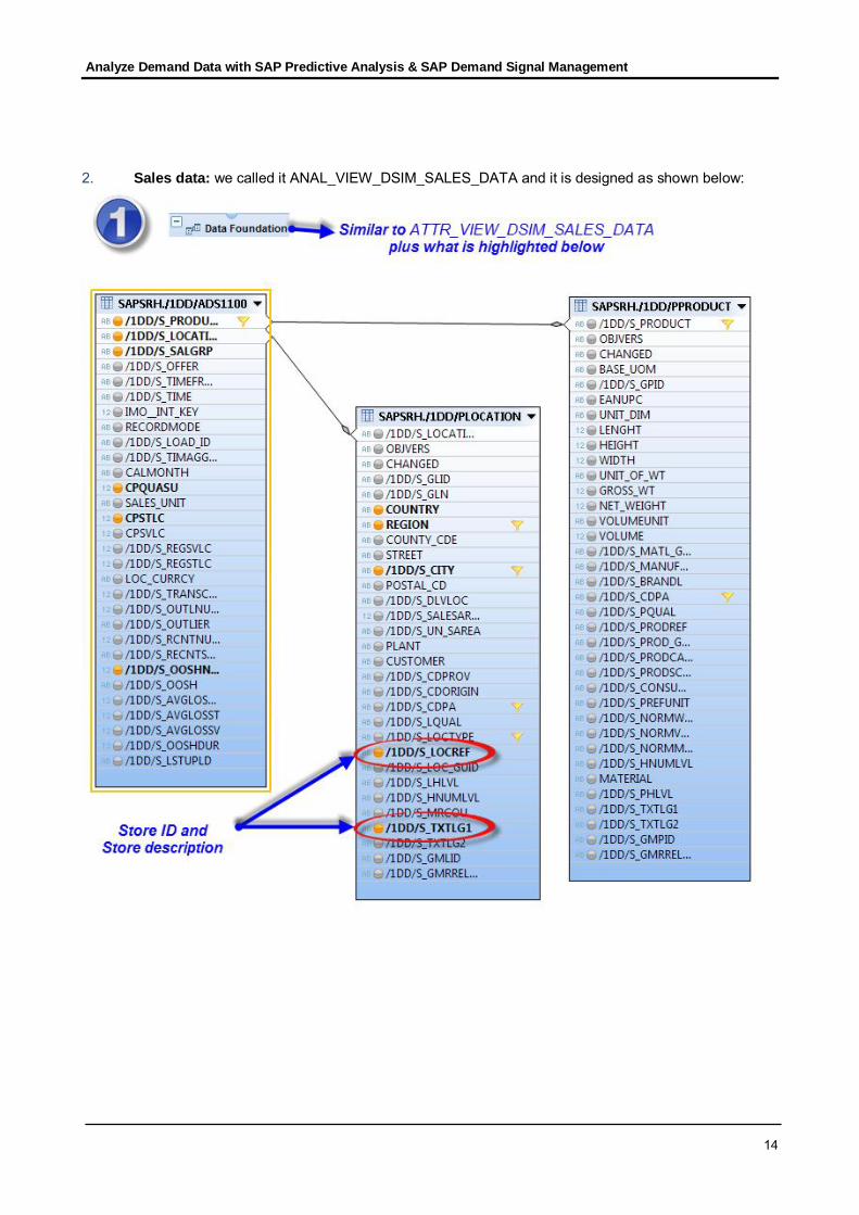
2. Sales data: we called it ANAL_VIEW_DSIM_SALES_DATA and it is designed as shown below:


15

Create Calculation ViewsIn this section we will describe the calculation view which is the frontend, or user interface, to our businesscase. Indeed, this is the view that we will be calling from the predictive analysis solution to fetch the requireddata. This calculation view will mainly:

1. do an union on the two previous analytical views to fetch the POS data2. format the selected data according to the data structure mentioned above

Step-by-Step Guide:

1. Use HANA Studio and create a Calculation view of type SQL Script. We called itCALC_VIEW_DSIM_POS_DATA

2. In the Script_View provide the necessary SQL Script, like the one shown below that consists of the 3main sections below and also highlighted in the SQL script:(1) Fetch the data and count the records or the data volume queried(2) Aggregate the data per location/Store(3) Format the data according to the output


16

/********* Begin Procedure Script ************/BEGIN--********************* (1) to count the records or the data volume queriedselect01 = SELECT"Location_int", "Product_int","Location", "Location_Description", "Country", "Region", "City","Stock","Out_Of_Stock","Promotion","Sales_Quantity","Sales_Revenue","Out_Of_Shelf"FROM "_SYS_BIC"."ab-data-pos/ANAL_VIEW_DSIM_STOCK_DATA";

select02 = SELECT"Location_int", "Product_int","Location", "Location_Description", "Country", "Region", "City","Stock","Out_Of_Stock","Promotion","Sales_Quantity","Sales_Revenue","Out_Of_Shelf"FROM "_SYS_BIC"."ab-data-pos/ANAL_VIEW_DSIM_SALES_DATA";

--Union sales and stockselect03 = CE_UNION_ALL(:select02,:select01);

--Count number of recordsvar_Records_Count = SELECT "Location", COUNT("Product_int") AS"Records_Number" FROM :select03 GROUP BY "Location";

--********************** (2) Aggregate the data per location/Storeselect1 = SELECT DISTINCT"Location_int","Location","Location_Description" AS "Store_Name","Country", "Region" AS "Region_key", "City",AVG("Stock") AS "Inventory", --calculate Stock averageSUM("Out_Of_Stock") AS "Out_of_stock",SUM("Promotion") AS "Promotion",SUM("Sales_Quantity") AS "Sales_Quantity",SUM("Sales_Revenue") AS "Sales_Revenue",SUM("Out_Of_Shelf") AS "Out_of_Shelf"FROM :select03GROUP BY "Location_int", "Location", "Location_Description", "Country","Region", "City"ORDER BY "Location_int" ASC, "Location" ASC, "Location_Description" ASC,"Country" ASC, "Region" ASC, "City" ASC;

--fetch the region descriptionselect2 = SELECT tbl_sales_data.*, tlb_region.TXTSH as "Region" FROM :select1as tbl_sales_dataINNER JOIN "SAPSRH"."/BI0/TREGION" AS tlb_regionON tbl_sales_data."Region_key" = tlb_region.REGION;


17

3. Complete the view, with the output below, save and activate

--************************* (3) Format the data according to the outputselect3= SELECTtbl_sales."Location" AS "Store_ID","Store_Name",SUM(tbl_sales."Out_of_Shelf") AS "OOSH_Count",SUM(tbl_sales."Promotion") AS "Promotion_Count",SUM(tbl_sales."Sales_Quantity") AS "Sales_Quantity",SUM(tbl_sales."Sales_Revenue") AS "Sales_Revenue",AVG(tbl_sales."Inventory") AS "Average_Inventory",SUM(tbl_sales."Out_of_stock") AS "OOST_Count",tbl_sales."Country",tbl_sales."Region",tbl_sales."City"FROM :select2 AS tbl_salesGROUP BY tbl_sales."Location", tbl_sales."Store_Name", tbl_sales."Country",tbl_sales."Region", tbl_sales."City"ORDER BY tbl_sales."Location", tbl_sales."Store_Name", tbl_sales."Country",tbl_sales."Region", tbl_sales."City" ASC;

var_out = SELECTtbl_output."Store_ID",tbl_output."Store_Name",tbl_output."OOSH_Count",tbl_output."Promotion_Count",tbl_output."Sales_Quantity",tbl_output."Sales_Revenue",tbl_output."Average_Inventory",tbl_output."OOST_Count",tbl_output."Country",tbl_output."Region",tbl_output."City",tbl_nbr."Records_Number" as "Sales_Records_Count"FROM :select3 as tbl_outputINNER JOIN :var_Records_Count as tbl_nbrON tbl_output."Store_ID" = tbl_nbr."Location"ORDER BY "Store_ID", "Store_Name", tbl_output."Country", tbl_output."Region",tbl_output."City" ASC;

END /********* End Procedure Script ************/


18

Predictive AnalysisNow that we have our final view CALCL_VIEW_DSIM_SALES_DATA that returns the data as requested forour described business use case, we can start the Predictive Analysis solution and follow the steps below toperform analysis on the DSiM POS data cross stores

1. Click on the button “New Document” in SAP Predictive Analysis Start Screen and choose “HANAOffline” as data source

Note: We use HANA Offline instead of the HANA Online connection since we want to replicate

data into PA. Indeed, analysis will be done in PA and not in HANA in this scenario. If, for any reason, your data is in an excel/CSV file, like for instance you uploaded data in

one of these files using the HANA views, you can also chose one of the related connectionsshown above.


19

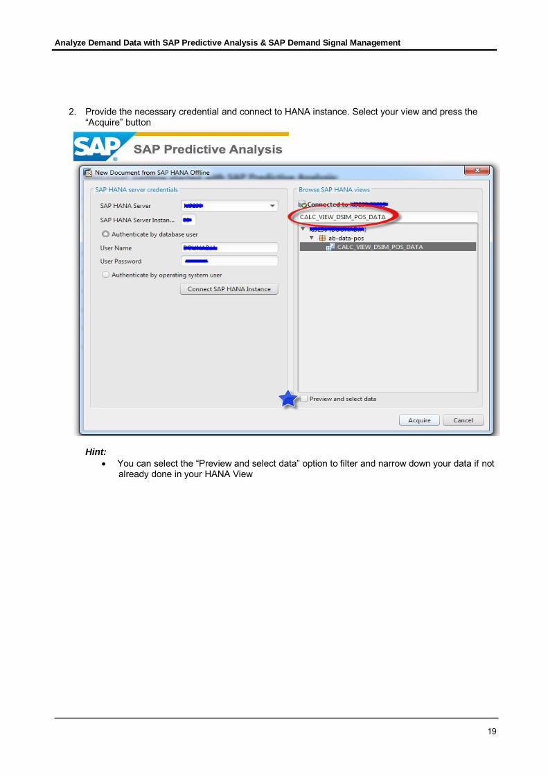
2. Provide the necessary credential and connect to HANA instance. Select your view and press the“Acquire” button

Hint: You can select the “Preview and select data” option to filter and narrow down your data if not

already done in your HANA View


20

Note:

After the first successful data acquisition, you will be able to connect to your view just bydouble clicking on it from the “Recent data source” section shown below:

Data VisualizationBelow you will find some alternatives to visualize the uploaded data. This section is optional and meantonly to provide you with some ideas on how to preview the data and also to highlight some selectedvisualization capabilities that are possible within PA. This will also help you to utilize the shown steps foryour own data visualization need.

1. to know POS data volume queried in HANA, you follow the steps highlighted below and dragand drop the records count measure (step 3), as shown below into the measures area

Note: This number represents the data volume queried, before being aggregated on store level

Hint: You can use the button “Save”, highlighted below, at the right bottom corner, to keep yourchart. Otherwise you will lose it if you chose another chart for visualization

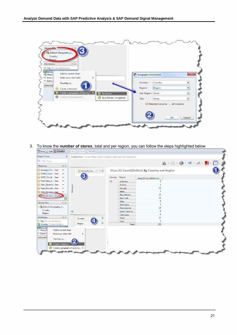
2. Create a geographic hierarchy using the two attributes “Country” and “Region”, as shownbelow, to visualize data using some Geographic Charts


21

3. To know the number of stores, total and per region, you can follow the steps highlighted below


22

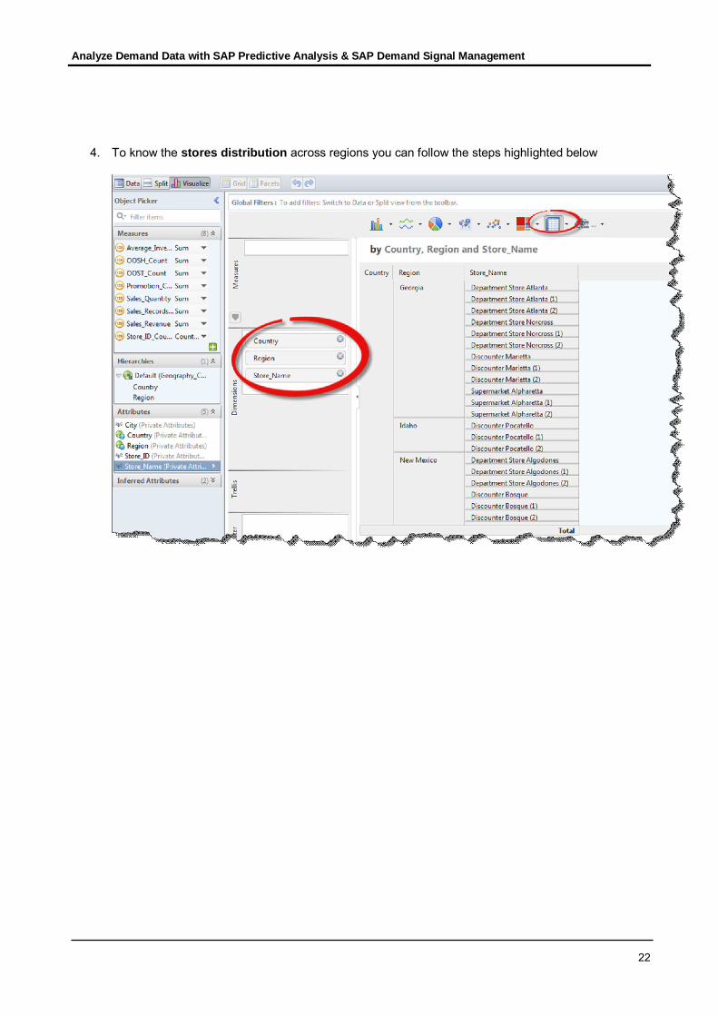
4. To know the stores distribution across regions you can follow the steps highlighted below


23

Hint:

You can filter the data, to show only stores for a given region. To do this, Drag and drop the“Region” onto the Filters pane, choose the required operator from the drop-down list, andselect the region value(s) you want to show/hide the related stores. Below for instance wehighlight only stores that belong to the region ”Texas”.


24

5. To have an idea about the number of Promotions, for the given product, performed per region useone of the geo charts as shown below:

6. Using the Tag Cloud chart, you can also have feeling about the highest Sales Revenue region


25

Note: at any time you can save your document. You will this way get a .SVID document that you canopen and complete later on and also share with others, if needed.

Data PreparationBefore proceeding with the data analysis, the SAP Predictive Analysis Solution allows you also tomanipulate your data if needed, for instance to:

Filter your data and this way apply the analysis only on the required data subset Create additional columns based on some calculation and/or data conversion Manipulate or change the data columns name and data type

For this, and much more, we suggest exploring the “Data Preparation” section that can be found in thearea “Predict”, highlighted below:

Data AnalysisTo access the analysis panel in PA you have to click ion the button “Predict” as shown below:

In this section we will describe the necessary steps to apply the K-Means algorithm, suggested by theData Analyst as mentioned in the business use case. We will show how to use and configure thisalgorithm within PA to cluster, for instance, the uploaded POS data, aggregated on store level, per groupof stores.


26

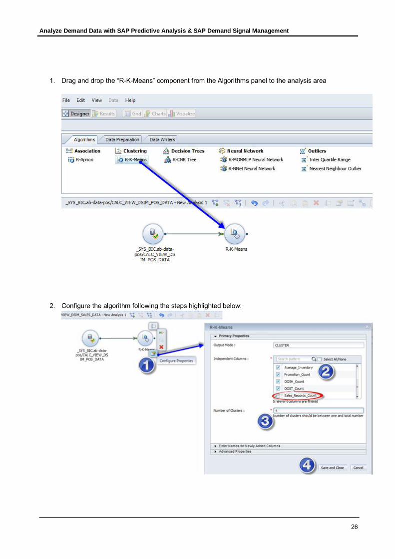
1. Drag and drop the “R-K-Means” component from the Algorithms panel to the analysis area

2. Configure the algorithm following the steps highlighted below:


27

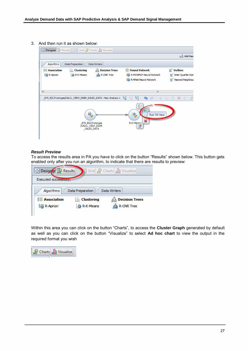
3. And then run it as shown below:

Result PreviewTo access the results area in PA you have to click on the button “Results” shown below. This button getsenabled only after you run an algorithm, to indicate that there are results to preview:

Within this area you can click on the button “Charts”, to access the Cluster Graph generated by defaultas well as you can click on the button “Visualize” to select Ad hoc chart to view the output in therequired format you wish


28

Result interpretation

In this section, we will first have an overview to the different existing cluster graphs and then take acloser look to the Radar chart to do a deeper analysis for each cluster and derive accurate actions thatthe situation requires. Afterwards, we will also share some ideas, and related “how to”, for some Ad hoccharts that can be useful as well

The Cluster Graph contains:• The size of the three clusters in the form of horizontal bar chart. You can change it to a pie chartor a vertical bar chart.


29

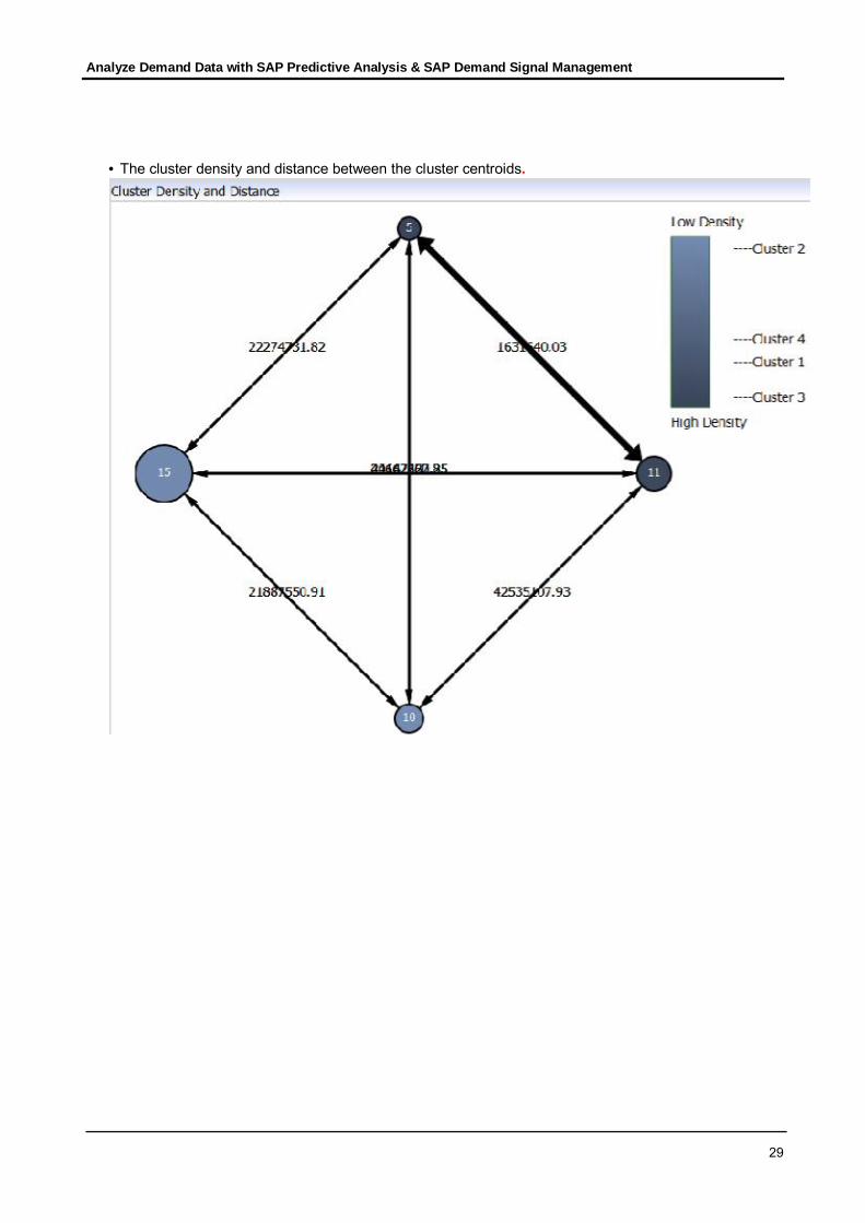
• The cluster density and distance between the cluster centroids.


30

• The independent variables of each cluster compared to the overall data in the area chart. TheVariable to be compared can be selected from the Variable drop-down list and the cluster can beselected from the Cluster slider.

• Cluster comparison using radar chart.

Click on the check-box “Normalize Results”. The cluster can be selected from the Cluster slider. Below,

as mentioned previously, analysis of each cluster and related action plan


31

Cluster 1

We can see that:- Number of Promotions is medium- Sales Revenue and quantity are high- No of Out-of-Shelf Situations is medium- No of Out-of-Stock Situations is high- Average inventory on-hand: low

This leads to the following conclusion:Stores, grouped in this cluster, could sell more than they currently do if we optimize the high rateof Out-of-Shelf and Out-of-Stock situations.Action items suggested:The Key Account Manager needs to talk to the retailer to increase the stock/inventory for thesestores. She/He could also work with his Supply Chain contact to further optimize thereplenishment planning and potentially schedule further deliveries.


32

Cluster 2

We can see that:- No of Promotion: very high- Sales Revenue and quantity: low- No of Out-of-Shelf Situations: low- No of Out-of-Stock Situations: high- Stock-on-Hand: high

This leads to the following conclusion:Even though there are a huge number of promotions running in these stores, there are issueswith the sales.Action items suggested:

The Key Account Manager needs to further analyze the promotion effectiveness of thepast promotions to check the root cause but also trigger onsite visits with salesrepresentatives to get the full picture of these stores. The stores might be located in low-sales regions with a low percentage of potential customers around.

Even though the stock-on-hand is high, there is still high number of out-of-stock signals.This is a sign that the stock-on-hand or out-of-stock signals are not consistent. In anycase, those stores need to be closely monitored.


33

Cluster 3

We can see that:- No of Promotion: medium- Sales Revenue and quantity: high- No of Out-of-Shelf Situations: low- No of Out-of-Stock Situations: low- Stock-on-Hand: medium

This leads to the following conclusion:Cluster 3 combines the top performing stores for the selected product.Action items suggested:

Analyze the effect of promotions on the sales in order to calculate the optimizedsales/promotion ratio. This could save future money if promotions are only run in thosestores if the increasing effect on sales is above a certain percentage.

Check the stock/sales ratio and find out whether the average stock level could bereduced in order to save the cost


34

Cluster 4

We can see that:- No of Promotions: high- Sales Revenue and quantity: low- No of Out-of-Shelf Situations: high- No of Out-of-Stock Situations: medium- Stock-on-Hand / Inventory: high

This leads to the following conclusion:Stores in this cluster face rather low sales compared to what was expected. The high inventorytells us that there might have been a drop in sales due to external factors that neither the retailernor manufacturer considered.Action items suggested:

Find out the root-causes to increase the sales and stop unnecessary replenishments inthe nearer future to avoid more stock on hand until the sales situation stabilized.

Overall, with the analysis of the four clusters, the key account manager has now some very detailedinformation and action items for the different stores. In some cases, she/he will need to work with the retailerto solve the issues and in some cases she/he can directly influence the situation.


35

Some Ad hoc charts:

1. List of stores in each cluster. With this information, the Key Account Manager can start toplan his action items easily. The table view of stores, with related region, in each cluster canbe visualized following the steps below:

a. Click on the button “Visualize”

b. Choose the table view

c. Drag and drop the “ClusterNumber”, “Region” and “Store_Name” attributes within theX Axis


36

2. List of stores for a given cluster. With this information, the Key Account Manager cannarrow down the stores list per cluster and hence par set of actions. You can follow thesame steps as in point 1 and then filter data as follows:

a. Drag and drop the “ClusterNumber” onto the Filters pane, choose the requiredoperator from the drop-down list, and select a value in the range slider. Below forinstance we highlight only stores that belong to cluster number 1


37

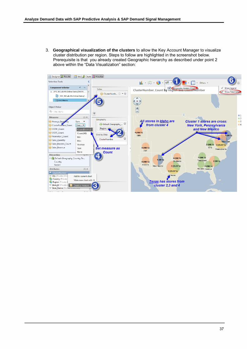
3. Geographical visualization of the clusters to allow the Key Account Manager to visualizecluster distribution per region. Steps to follow are highlighted in the screenshot below.Prerequisite is that you already created Geographic hierarchy as described under point 2above within the “Data Visualization” section:


38

Result PersistencyBeside the predictive capabilities and the various useful visualization features, SAP PredictiveAnalysis solution allows you also to preserve your data and the analysis results into a given storagearea. For this we suggest exploring the “Data Preparation” section, under Predict, highlighted below:

Using the JDBC Writer component that you can configure as shown below, you will be able towrite the required data back into HANA:

Hint:You can follow what was described under the “Data Preparation” section to manipulate yourdata if needed before storage


39

SCENARIO 2: PREDICTIVE ANALYSIS WITHIN SAP HANA AND DATA VISUALIZATION WITH THESAP PA SOLUTION

In the second scenario, predictive analysis is performed directly in HANA, leveraging the PAL(Predictive Analysis Library) as well as the power of in-memory data mining capabilities for handlinglarge data volumes. The results are then extracted to the SAP Predictive Analysis solution to utilize theinteractive data visualization capabilities of PA through some very useful and known charts. This is doneusing HANA stored procedures and HANA Views.In comparison with the first scenario above, this approach has the following advantages:

Besides the predictive analysis capabilities provided by PA (like in the first scenario), you can inaddition leverage all the predictive capabilities powered by HANA:

all algorithms available in PAL and BFL library though the HANA R integration, it is possible to use all the R packages/algorithms

All the DSiM data is available for the predictive analysis and it is possible to leverage the HANAplatform to process Big data in DSiM. You therefore can overcome the data volume restrictions ofPA.

This approach ensures more predictive capability, more sophisticated data processing and processing bigdata volume.

Architectural Approach

Prerequisites

1. Use SAP Predictive Analysis 1.0.10 or later releases.2. SAP HANA SPS05 or later releases.3. Install the Application Function Library (AFL), which includes PAL. For more information, please refer

to the SAP HANA Server Installation Guide.http://help.sap.com/hana/SAP_HANA_Server_Installation_Guide_en.pdfCan be helpful to take a look at SAP HANA Predictive Analysis Library (PAL) Reference document:


40

https://help.sap.com/hana/hana_dev_pal_en.pdf4. Can be helpful to take a look at the SAP Predictive Analysis user guide:

http://help.sap.com/pa


41

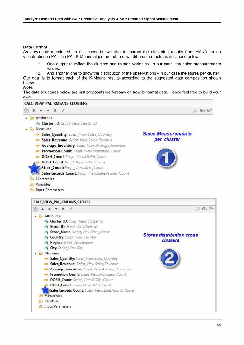
Data FormatAs previously mentioned, in this scenario, we aim to extract the clustering results from HANA, to dovisualization in PA. The PAL K-Means algorithm returns two different outputs as described below:

1. One output to reflect the clusters and related variables- in our case, the sales measurementsvalues.

2. And another one to show the distribution of the observations - in our case the stores per clusterOur goal is to format each of the K-Means results according to the suggested data composition shownbelow:Note:The data structures below are just proposals we foresaw on how to format data. Hence feel free to build yourown.


42

Note:Store_Count and SalesRecords_Count, highlighted above, are optional to have, as they are not partof the PAL K-Means results. Nevertheless, they might be good to have, to allow us to know thenumber of stores per cluster and to assess the data volume handled.

In the following section we will list the necessary HANA views to extract such data and also give some highlevel technical guidance on how to build them and on how to use PAL.HANA ViewsTo extract predictive analysis results, the HANA views below can be usedNote:

This section is not intended as a general presentation of the HANA Views. As well, the approach todesign/create HANA views, described in the coming sections is not the unique possible one. It is rather toillustrate a simplified approach that we followed to extract and prepare the DSiM data for the use ofpredictive capability provided in PA & HANA, according to the data format we set above.

SQL Script to Call PAL K-Means

To use PAL functions, we must do the following first:

1. Create the AFL_WRAPPER_GENERATOR procedure. This only needs to be done once.2. From within SQLScript code, generate a procedure that wraps the PAL function.3. Call the procedure, for example, from an SQL Script procedure.

In the following section we will describe step 1 and 2 above whereas step 3 will be covered under thedifferent HANA views sections since for each of the data format we wanted to cover, the procedure call maydiffer.


43

Step 1 – Create the AFL_WRAPPER_GENERATOR ProcedureBefore using any AFL function, you need to create the AFL_WRAPPER_GENERATOR procedure. For moredetails on how to achieve this we recommend you take a look to section ` Create theAFL_WRAPPER_GENERATOR Procedure ` within the SAP HANA Predictive Analysis Library (PAL)Reference document mentioned in the”Prerequisites” chapter.

Step 2 – Generate a PAL ProcedureAny user granted with the EXECUTE privilege on the system.afl_wrapper_generator procedure can generatea procedure for a specific PAL function. The generic syntax is described in the SAP HANA PredictiveAnalysis Library (PAL) Reference document we mention above. Below, we will be showing and detailing theversion adjusted to our use case.The SQL script is structured as described in the points below and you can find the SQL section related toeach point within the complete SQL script right after:

A. Define format of Data to ClusterWithin this step we define the structure/format of the data, we will be clustering meaning that we willbe submitting to K-Means, and create the related table type

B. K-Means configurationWithin this step we:

a. Define the table type, and create the related DB table, to set Parameters for PALAlgorithm/Function K-Means

b. Fill the created DB table with the necessary settings, like number of clusters, to configure theK-Means algorithm

Note: You need to re-run step b each time you want to change or re-set K-Means configuration

Hint: In case you want to run K-Means with different settings we suggest you create a DB table for eachsetting. This way you can switch from testing one setting to another easily.

C. K-Means output/resultsAs mentioned above, the PAL K-Means algorithm returns, as output, two tables as described below:

a. One table that holds the distribution of the observations, in our case the stores, per clustersb. And another table that holds the clusters and related variables, in our case the sales

measurements, values. This tale is also called centers’ table

In this section we create the table type for each result. We haveDSIM_POS_DATA_KMEANS_STORES_T for point a and DSIM_POS_DATA_KMEANS_CLUSTERS_T for point b

D. Create PAL procedure for K-MeansAt this level, we have all the necessary HANA content, as per the PAL syntax and our use caserequirements to call K-Means on the DSiM POS data. Hence, we just create the PAL procedure thatcan be called later on in our views to perform data clustering


44

/********SQL Script to Create the PAL Clustering Algorithm K-Means Procedure******/

SET SCHEMA _SYS_AFL;--> All the used/created content is under schema _SYS_AFL

--************************* (1) DATA to apply K-Means on (Data to cluster)--TYPEDROP TYPE DSIM_POS_DATA_TAB_T;CREATE TYPE DSIM_POS_DATA_TAB_T AS TABLE("ID" VARCHAR (10), -->must be called ID but in fact represents Store id for our case"OOSH_Count" INTEGER,"Promotion_Count" INTEGER,"Sales_Quantity" DOUBLE,"Sales_Revenue" DOUBLE,"Average_Inventory" DOUBLE,"OOST_Count" DOUBLE,PRIMARY KEY("ID"));--************************** (2) Parameters for PAL Algorithm K-Means-- (K-Means configuration)--TYPEDROP TYPE DSIM_POS_DATA_KMEANS_PAMAMETERS_T;CREATE TYPE DSIM_POS_DATA_KMEANS_PAMAMETERS_T AS TABLE("NAME" VARCHAR (50),"INTARGS" INTEGER,"DOUBLEARGS" DOUBLE,"STRINGARGS" VARCHAR (100));

--TABLEDROP TABLE DSIM_POS_DATA_KMEANS_PAMAMETERS_TAB;CREATE COLUMN TABLE DSIM_POS_DATA_KMEANS_PAMAMETERS_TAB("NAME" VARCHAR (50),"INTARGS" INTEGER,"DOUBLEARGS" DOUBLE,"STRINGARGS" VARCHAR (100));

--Parameters values/setting (K-Means configuration)INSERT INTO DSIM_POS_DATA_KMEANS_PAMAMETERS_TABVALUES ('THREAD_NUMBER',2,null,null);INSERT INTO DSIM_POS_DATA_KMEANS_PAMAMETERS_TABVALUES ('GROUP_NUMBER',4,null,null);-->number of clustersINSERT INTO DSIM_POS_DATA_KMEANS_PAMAMETERS_TABVALUES ('INIT_TYPE',4,null,null);INSERT INTO DSIM_POS_DATA_KMEANS_PAMAMETERS_TABVALUES ('DISTANCE_LEVEL',2,null,null);INSERT INTO DSIM_POS_DATA_KMEANS_PAMAMETERS_TABVALUES ('MAX_ITERATION',100,null,null);INSERT INTO DSIM_POS_DATA_KMEANS_PAMAMETERS_TABVALUES ('EXIT_THRESHOLD',null,0.000001,null);INSERT INTO DSIM_POS_DATA_KMEANS_PAMAMETERS_TABVALUES ('NORMALIZATION',2,null,null);--> This is to normalize results-- and make the values between 0 and 1


45

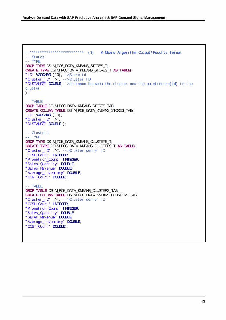
--************************** (3) K-Means Algorithm Output/Results format-- Stores-- TYPEDROP TYPE DSIM_POS_DATA_KMEANS_STORES_T;CREATE TYPE DSIM_POS_DATA_KMEANS_STORES_T AS TABLE("ID" VARCHAR (10),-->Store id"Cluster_ID" INT, -->Cluster ID"DISTANCE" DOUBLE -->distance between the cluster and the point/store(id) in thecluster);

-- TABLEDROP TABLE DSIM_POS_DATA_KMEANS_STORES_TAB;CREATE COLUMN TABLE DSIM_POS_DATA_KMEANS_STORES_TAB("ID" VARCHAR (10),"Cluster_ID" INT,"DISTANCE" DOUBLE );

-- Clusters-- TYPEDROP TYPE DSIM_POS_DATA_KMEANS_CLUSTERS_T;CREATE TYPE DSIM_POS_DATA_KMEANS_CLUSTERS_T AS TABLE("Cluster_ID" INT, -->Cluster center ID"OOSH_Count" INTEGER,"Promotion_Count" INTEGER,"Sales_Quantity" DOUBLE,"Sales_Revenue" DOUBLE,"Average_Inventory" DOUBLE,"OOST_Count" DOUBLE);

-- TABLEDROP TABLE DSIM_POS_DATA_KMEANS_CLUSTERS_TAB;CREATE COLUMN TABLE DSIM_POS_DATA_KMEANS_CLUSTERS_TAB("Cluster_ID" INT, -->Cluster center ID"OOSH_Count" INTEGER,"Promotion_Count" INTEGER,"Sales_Quantity" DOUBLE,"Sales_Revenue" DOUBLE,"Average_Inventory" DOUBLE,"OOST_Count" DOUBLE);


46

-- *************************** (4) Create PAL procedure for K-Means--Create the input table for the procedureDROP TABLE DSIM_POS_DATA_KMEAN_PROCED_INPUT;CREATE COLUMN TABLE DSIM_POS_DATA_KMEAN_PROCED_INPUT("ID" INT,"TYPENAME" VARCHAR(100),"DIRECTION" VARCHAR(100) );

--Submit the different procedure’s input/output tables' typeINSERT INTO DSIM_POS_DATA_KMEAN_PROCED_INPUTVALUES (1, '_SYS_AFL.DSIM_POS_DATA_TAB_T', 'in');INSERT INTO DSIM_POS_DATA_KMEAN_PROCED_INPUTVALUES (2, '_SYS_AFL.DSIM_POS_DATA_KMEANS_PAMAMETERS_T', 'in');INSERT INTO DSIM_POS_DATA_KMEAN_PROCED_INPUTVALUES (3, '_SYS_AFL.DSIM_POS_DATA_KMEANS_STORES_T', 'out');INSERT INTO DSIM_POS_DATA_KMEAN_PROCED_INPUTVALUES (4, '_SYS_AFL.DSIM_POS_DATA_KMEANS_CLUSTERS_T', 'out');

--Drop previous procedure if anyDROP PROCEDURE DSIM_POS_DATA_PAL_KMEANS;DROP TYPE DSIM_POS_DATA_PAL_KMEANS__TT_P1;DROP TYPE DSIM_POS_DATA_PAL_KMEANS__TT_P2;DROP TYPE DSIM_POS_DATA_PAL_KMEANS__TT_P3;DROP TYPE DSIM_POS_DATA_PAL_KMEANS__TT_P4;

--Create the procedure to call the PAL function KMEANSCALL SYSTEM.AFL_WRAPPER_GENERATOR('DSIM_POS_DATA_PAL_KMEANS', 'AFLPAL', 'KMEANS',DSIM_POS_DATA_KMEAN_PROCED_INPUT);


47

Create Attribute ViewsSame concept and technical steps/details described under Create Attribute View for Scenario 1 aboveCreate Analytic ViewsSame concept and technical steps/details described under Create Attribute View for Scenario 1 aboveCreate Calculation ViewsNote:You must execute the SQL Script to Generate a PAL Procedure before you create the views describedbelow

A. HANA view to output the Clusters

1. Use HANA Studio and create a Calculation view of type SQL Script. We called itCALC_VIEW_PAL_KMEANS_CLUSTERS.

Note: You must set schema to “_SYS_AFL” in the view properties as shown below:

2. In the Script View provide the necessary SQL Script, like the one shown below, to call the PAL K-Means function


48

/** Apply K-Means, on DSiM POS Data, using PAL - Returns Clusters Results **//********* Begin Procedure Script ************/BEGIN/* NOTE: - Default schema _SYS_AFL is set in the properties of the procedure - Assumption is that all necessary types, tables and K-Means Stored Procedure (with necessary input parameters) are created in advance*/--**************** (1) Fetch data to be used as input for KMEANS algorithm--********** (A) to count the records or the data volume queriedselect01 = SELECT"Location_int", "Product_int","Location", "Location_Description", "Country", "Region", "City","Stock","Out_Of_Stock","Promotion","Sales_Quantity","Sales_Revenue","Out_Of_Shelf"FROM "_SYS_BIC"."ab-data-pos/ANAL_VIEW_DSIM_STOCK_DATA";


--Union sales and stock recordsselect03 = CE_UNION_ALL(:select02,:select01);

--Count number of records per storevar_Records_Count = SELECT "Location" , COUNT("Product_int") AS"SalesRecords_Count" FROM :select03 GROUP BY "Location";

--************* (B) Aggregate the data per location/Storevar_sales_data = SELECT DISTINCT"Location_int" AS "ID",AVG("Stock") AS "Average_Inventory",SUM("Out_Of_Stock") AS "OOST_Count",SUM("Promotion") AS "Promotion_Count",SUM("Sales_Quantity") AS "Sales_Quantity",SUM("Sales_Revenue") AS "Sales_Revenue",SUM("Out_Of_Shelf") AS "OOSH_Count"FROM :select03GROUP BY "Location_int"ORDER BY "Location_int" ASC;


49

3. Complete the view with the output below. Save and activate.

--**************** (2) Fetch the parameters from PAL procedurevar_parameters = SELECT * FROM DSIM_POS_DATA_KMEANS_PAMAMETERS_TAB;

--The following is a dummy internal table that is necessary to initialize thestructure of K-Means resultsvar_results_stores = SELECT TOP 0 * FROM DSIM_POS_DATA_KMEANS_STORES_TAB;var_results_clusters = SELECT TOP 0 * FROM DSIM_POS_DATA_KMEANS_CLUSTERS_TAB;

--***************** (3) Call the wrapper stored procedure for the PAL K-MeansCALL DSIM_POS_DATA_PAL_KMEANS(:var_sales_data, :var_parameters,:var_results_stores , :var_results_clusters);

--***************** (4) Format results for outputvar_store_Number = SELECT "Cluster_ID", COUNT("ID") AS "Store_Count" FROM:var_results_stores GROUP BY "Cluster_ID";

var_records_Number = SELECT "Location_int" AS "ID", COUNT("Product_int") AS"SalesRecords_Count" FROM :select03 GROUP BY "Location_int";

var_tab1 = CE_JOIN(:var_records_Number, :var_results_stores, ["ID"],["ID","Cluster_ID","SalesRecords_Count"]);

var_tab2 = SELECT "Cluster_ID", SUM("SalesRecords_Count") AS"SalesRecords_Count" FROM :var_tab1 GROUP BY "Cluster_ID";

var_out_tmp =CE_JOIN(:var_store_Number, :var_tab2,["Cluster_ID"],["Cluster_ID","Store_Count","SalesRecords_Count"]);

var_out = CE_JOIN(:var_results_clusters, :var_out_tmp, ["Cluster_ID"],["Cluster_ID","Store_Count","OOSH_Count","Promotion_Count","Sales_Quantity","Sales_Revenue","Average_Inventory","OOST_Count","SalesRecords_Count"]);

END /********* End Procedure Script ************/


50

B. HANA view to output the Stores per clusters

1. Use HANA Studio and create a Calculation view of type SQL Script. We called itCALC_VIEW_PAL_KMEANS_STORES.

Note: You must set schema to “_SYS_AFL” in the view properties as shown below:


51

2. In the Script View provide the necessary SQL Script, like the one shown below, to call the PAL K-Means function.

Note: You can reuse part (1.A), (2) and (3) from the SQL Script for clusters view described above/** Apply K-Means, on DSiM POS Data, using PAL - Returns Clusters Results **/

/********* Begin Procedure Script ************/BEGIN/* NOTE: - Default schema _SYS_AFL is set in the properties of the procedure - Assumption is that all necessary types, tables and K-Means Stored Procedure (with necessary input parameters) are created in advance*/--**************** (1) Fetch data to be used as input for KMEANS algorithm--********** (A) to count the records or the data volume queriedselect01 = SELECT"Location_int", "Product_int","Location", "Location_Description", "Country", "Region", "City","Stock","Out_Of_Stock","Promotion","Sales_Quantity","Sales_Revenue","Out_Of_Shelf"FROM "_SYS_BIC"."ab-data-pos/ANAL_VIEW_DSIM_STOCK_DATA";


--Union sales and stock recordsselect03 = CE_UNION_ALL(:select02,:select01);

--Count number of records per storevar_Records_Count = SELECT "Location" , COUNT("Product_int") AS"SalesRecords_Count" FROM :select03 GROUP BY "Location";


52

--************* (B) Aggregate the data per location/Store-- Fetch the region descriptionselect04 = select tbl_sales_data.*, tlb_region.TXTSH as "Region" from :select03AS tbl_sales_dataINNER JOIN "SAPSRH"."/BI0/TREGION" as tlb_regionon tbl_sales_data."Region_key" = tlb_region.REGION;

var_sales_data = SELECT"Store_ID" as "ID", "Country", "Region", "Store_Name", "City",AVG("Stock") AS "Average_Inventory",SUM("Out_Of_Stock") AS "OOST_Count",SUM("Promotion") AS "Promotion_Count",SUM("Sales_Quantity") AS "Sales_Quantity",sum("Sales_Revenue") AS "Sales_Revenue",sum("Out_Of_Shelf") AS "OOSH_Count"FROM :select04GROUP BY "Store_ID","Country", "Region","Store_Name","City"ORDER BY "Store_ID","Country", "Region","Store_Name","City" ASC;

--**************** (2) Fetch the parameters from PAL procedurevar_parameters = SELECT * FROM DSIM_POS_DATA_KMEANS_PAMAMETERS_TAB;

-- Dummy internal table necessary to initialize the structure of K-Means resultsvar_results_stores = SELECT TOP 0 * FROM DSIM_POS_DATA_KMEANS_STORES_TAB;var_results_clusters = SELECT TOP 0 * FROM DSIM_POS_DATA_KMEANS_CLUSTERS_TAB;

--***************** (3) Call the wrapper stored procedure for the PAL algorithmCALL DSIM_POS_DATA_PAL_KMEANS(:var_sales_data, :var_parameters,:var_results_stores , :var_results_clusters);

--***************** (4) Format results for output--count number of sales records per storevar_count_sales_records = SELECT "Store_ID" AS "ID", COUNT("Product_int") AS"SalesRecords_Count" FROM :select03 GROUP BY "Store_ID";

--Increase cluster number by 1 to avoid having zero as cluster numbervar_results_stores = SELECT "ID", "Cluster_ID" + 1 as "Cluster_ID", "DISTANCE" from :var_results_stores;var_results_clusters = SELECT "Cluster_ID" + 1 as "Cluster_ID",

"OOSH_Count", "Promotion_Count","Sales_Quantity","Sales_Revenue","Average_Inventory","OOST_Count"from :var_results_clusters;

--assign sales records to store/clustervar_tab1 = CE_JOIN(:var_count_sales_records, :var_results_stores, ["ID"],["ID","Cluster_ID","SalesRecords_Count"]);

--format outputvar_out = selecttbl_kmeans_stores."Cluster_ID", tbl_sales_data."OOSH_Count" ,tbl_sales_data."Promotion_Count" , tbl_sales_data."Sales_Quantity",tbl_sales_data."Sales_Revenue" , tbl_sales_data."Average_Inventory" ,tbl_sales_data."OOST_Count", tbl_kmeans_stores."SalesRecords_Count",tbl_sales_data."ID" as "Store_ID", "Store_Name", "Country", "Region", "City"from :var_sales_data as tbl_sales_dataINNER JOIN :var_tab1 as tbl_kmeans_storesON tbl_sales_data."ID" = tbl_kmeans_stores."ID" ;END /********* End Procedure Script ************/


53

3. Complete the view with the output below. Save and activate.


54

Predictive AnalysisNow that we have the necessary views (for clusters and stores) to call the PAL K-Means, we will describe, inthe sections below how to use the Predictive Analysis solution to perform analysis on the DSiM POS dataacross stores.

1. Click on the button “New Document” and chose “HANA Offline” as data source

Note:We use HANA Offline, instead of HANA Online, connection since the PAL K-Means, iscalled/executed beforehand in the HANA view. In PA we will export the results to perform datavisualization and analysis through the various visualization capabilities provided or possible


55

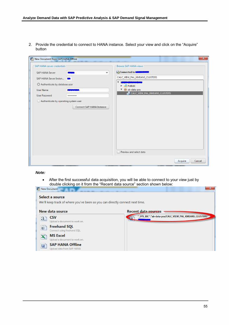
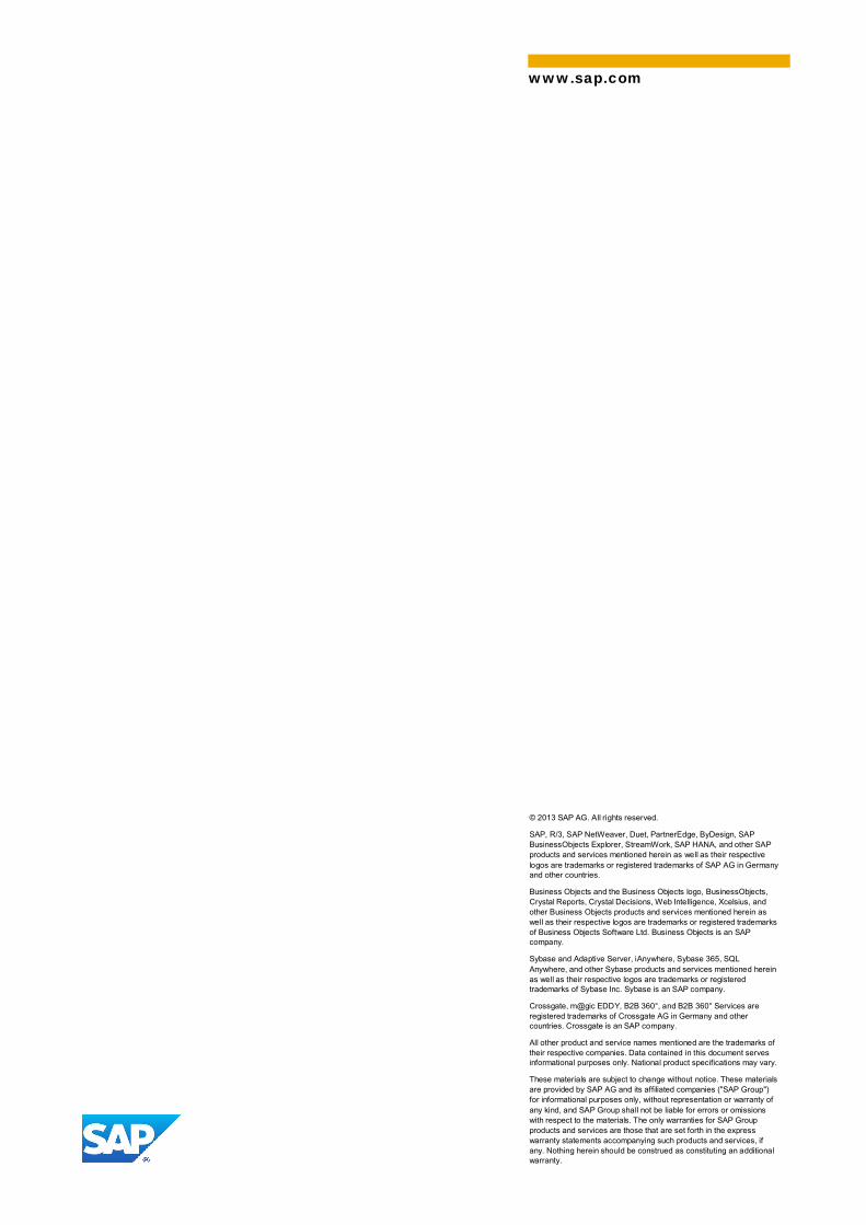
2. Provide the credential to connect to HANA instance. Select your view and click on the “Acquire”button

Note:

After the first successful data acquisition, you will be able to connect to your view just bydouble clicking on it from the “Recent data source” section shown below:


56

Data Visualization

To avoid redundancy, we suggest you take a look to the Data Visualization section for the first scenario andtry to apply it at your conveniences.

Result AnalysisIn this section we will try to perform similar data analysis, described for scenario 1, under “Result”interpretation section.As you might have already guessed, we don’t have default charts, as it was the case for scenario1. We willtherefore need to build them by ourselves.

Note:We will mainly focus on the following charts or data representations:

1. Clusters size: to get an idea of store numbers per cluster

2. the Radar chart, to allow us do a deeper analysis for each cluster and derive accurate actions thatthe situation requires

3. Store distribution per cluster: to help the Key Account Manager to start to plan his action itemseasily

For the charts analysis part, and for sake to avoid redundancy, we suggest you take a look at the Resultinterpretation section for the first scenario and try to do same here.

1. Clusters size: as shown below, it represents number of stores per cluster and can be achieved byfollowing the steps highlighted in the screenshot below

2. Radar chart: as shown below, it represents number of stores per cluster and can be achieved byfollowing the steps highlighted in the screenshot below


57

Hint:To display the Radar chart per cluster you can use one of the options below:A – Make usage of the filter as highlighted below and set the clutter ID you want to display

B – Make usage of the “Trellis” area/feature, as highlighted below, either per Row (first screenshot) or byColumn (second screenshot)


58


59

3. Store distribution per cluster: for this part of analysis you need to:a. Connect to the stores calculation view CALC_VIEW_PAL_KMEANS_STORES describe

aboveb. Refer to the part “Some Ad hoc charts”, under the Result interpretation section to build

necessary charts

Result PersistencyYou need to persist the data. You can follow what is described under same section for scnerio1.

Data Preparation

In case you need to perform any manipulation to the data/results you uploaded, we also suggest you take alook to the Data Preparation section for the first scenario and try to apply it at your conveniences.

COMPLIANCY

The two scenarios utilize HANA views created on-top-of BW Tables. Hence:

1. It is to clarify whether the HANA (and DSiM) license agreement is applicable for this kind of HANAusage.

2. Please check the SAP note 1682131 for detailed information about the restriction of this kind ofusage of BW tables. This SCN document will be updated once the alternative BW/HANA feature (i.e.the so-called OLAP Views based on BW tables) described in this note, are available.

3. The 2 scenarios described in this doc focus on leveraging predictive capability in HANA, the BWauthorizations and DSiM authorizations could not be used. In this case the HANA privileges shouldbe used to control the access of DSiM data. Please consider to use HANA privileges to control theaccess of DSiM data.

ADDITIONAL LINKS

SCN community link for PA: http://scn.sap.com/community/predictive-analysisSAP Predictive Analysis User Guide: http://help.sap.com/paSAP HANA Server Installation Guide (Installing Application Function Libraries (AFLs)):http://help.sap.com/hana/SAP_HANA_Server_Installation_Guide_en.pdfSAP HANA Predictive Analysis Library (PAL) Reference document:https://help.sap.com/hana/hana_dev_pal_en.pdf

© 2013 SAP AG. All rights reserved.

SAP, R/3, SAP NetWeaver, Duet, PartnerEdge, ByDesign, SAPBusinessObjects Explorer, StreamWork, SAP HANA, and other SAPproducts and services mentioned herein as well as their respectivelogos are trademarks or registered trademarks of SAP AG in Germanyand other countries.

Business Objects and the Business Objects logo, BusinessObjects,Crystal Reports, Crystal Decisions, Web Intelligence, Xcelsius, andother Business Objects products and services mentioned herein aswell as their respective logos are trademarks or registered trademarksof Business Objects Software Ltd. Business Objects is an SAPcompany.

Sybase and Adaptive Server, iAnywhere, Sybase 365, SQLAnywhere, and other Sybase products and services mentioned hereinas well as their respective logos are trademarks or registeredtrademarks of Sybase Inc. Sybase is an SAP company.

Crossgate, m@gic EDDY, B2B 360°, and B2B 360° Services areregistered trademarks of Crossgate AG in Germany and othercountries. Crossgate is an SAP company.

All other product and service names mentioned are the trademarks oftheir respective companies. Data contained in this document servesinformational purposes only. National product specifications may vary.

These materials are subject to change without notice. These materialsare provided by SAP AG and its affiliated companies ("SAP Group")for informational purposes only, without representation or warranty ofany kind, and SAP Group shall not be liable for errors or omissionswith respect to the materials. The only warranties for SAP Groupproducts and services are those that are set forth in the expresswarranty statements accompanying such products and services, ifany. Nothing herein should be construed as constituting an additionalwarranty.

www.sap.com

Analyze Demand Data with SAP Predictive Analysis & SAP ... · PDF fileAnalyze Demand Data with...

Documents

Transcript of Analyze Demand Data with SAP Predictive Analysis & SAP ... · PDF fileAnalyze Demand Data with...