Analyticity of solutions to nonlinear

parabolic equations on manifolds and

an application to Stokes flow

Joachim Escher and Georg Prokert

Dedicated to Herbert Amann on the occasion of his 65th birthday

Abstract

We prove a general regularity result for fully nonlinear, possibly nonlocalparabolic Cauchy problems under the assumption of maximal regularityfor the linearized problem. We apply this result to show joint spatial andtemporal analyticity of the moving boundary in the problem of Stokesflow driven by surface tension.

Key words: nonlinear parabolic equation, maximal regularity, Stokesflow, surface tension

AMS subject classification: 35K55, 35Q30, 35R35, 76D07

1 Introduction

The theory of maximal regularity for (linear) parabolic evolution equations hasproved itself to be a powerful tool for the treatment of nonlinear parabolic prob-lems ( see [2, 3, 18] e.a.). In a functional analytic framework of function spaces inwhich this theory is applicable, questions of existence, uniqueness, ”linearizedstability analysis”, existence of invariant manifolds etc. can be treated to agreat extent in a fashion similar as in the case of (finite dimensional) ordinarydifferential equations.

Of course, an additional issue for parabolic equations is the smoothing prop-erty of the evolution: A function satisfying a parabolic Cauchy problem will be”as smooth as the operator and the right-hand side will allow” immediately afterthe initial time. The classical method of proving this in the case of quasilinearequations is by ”bootstrapping”, i.e. proving higher smoothness of an alreadyestablished solution inductively by invoking smoothness results for linear equa-tions in every step. One encounters considerable technical difficulties, however,when one tries to apply this technique to fully nonlinear problems and to theproof of analyticity in space.

1

In [3, 4], Angenent introduced a different approach to the proof of thesmoothing property, relying also on the maximal regularity property: By in-troducing two parameters representing a scaling in time and a translation inspace, respectively, the desired smoothness result follows immediately from theImplicit Function theorem. More precisely, this theorem yields smooth depen-dence of the solution of the parameter-dependent problem on the parameters,and this can be straightforwardly translated to a smoothness result (in spaceand time) for the solution of the original problem. This elegant and transparentapproach is immediately applicable to fully nonlinear problems and also yieldsanalyticity of the solution. Besides the framework of maximal regularity, thecrucial condition for its applicability is the equivariance of the evolution op-erator with respect to translations. For an application of this approach to aproblem on Rn, see [10].

In subsequent work, Angenents idea has been generalized to apply it tobroader problem classes. In [13], a localized version is given which can beused to establish regularity properties (including analyticity) for solutions ofparabolic (as well as elliptic) differential equations on domains in Rn. In [12],evolution equations on an arbitrary symmetric space are considered, where theunderlying Lie group plays the role of the group of translations in the caseof Rn. Both in [12] and [13], the equivariance condition is relaxed to a morenatural assumption which allows, for example, to treat differential operatorswith variable coefficients.

It is the first aim of the present paper to generalize the idea described aboveeven further. We present a set of conditions on a family of flows on a manifoldwhich enable us to perform this ”parameter trick”, and we show the existenceof such a family if the underlying manifold is compact. Then a general resulton the smoothing property for abstract parabolic evolution equations is shown.As our main interest is in analyticity here, the assumptions and results areformulated in the Cω-class. It is clear, however, that the same techniques arealso applicable in lower smoothness classes.

The second part of the present paper is devoted to an application of ourabstract result to a moving boundary problem occurring in low Reynolds numberflow. The application is nontrivial in two senses: The result we prove is new, andin the general case it cannot be obtained via previous versions of the parametertrick. We consider the deformation of a liquid drop driven by the capillaryforces on its boundary. The velocity and pressure fields inside the drop aregoverned by the (homogeneous and incompressible) Stokes equations, and theboundary of the drop moves according to the velocity field. The influence ofthe capillary forces is modelled by a so-called traction boundary condition, i.e.a dynamic boundary condition relating the curvature to the stress tensor. Forthe precise problem formulation as well as for references to previous results onthis problem, we refer to Section 5. We show that the boundary of the movingdrop becomes analytic in space and time immediately. It should be pointedout that substantial parts of the analysis which is carried out here are in factnot particular to the discussed problem. Various techniques can be used also inparallel investigations of other (nonlocal) parabolic moving boundary problems.

2

This paper is organized as follows: In Section 2, the basic facts on continuousmaximal regularity are reviewed. The abstract key result is proved in Section 3.Section 4 contains a series of technical results on the smoothness of a parameter-dependent pull-back, considered as a function of the parameter. These resultsare essentially parallel to the following prototype: For u ∈ BUC(R), k ∈ N, themapping [µ 7→ u(· + µ)] is in Ck(R, BUC(R)) if (and only if) u ∈ BUCk(R).The results as well as their proofs are oriented at [13]. Finally, the applicationof the abstract result to the Stokes flow problem is carried out in Section 5.Here, two independent results on the Stokes equation with traction boundaryconditions in little Holder spaces on a fixed, smooth domain are used. These areproved in Appendix A. Finally, we also need a generation result on little Holderspaces for an operator which is the sum of the Dirichlet-Neumann operator forthe Laplacian and a first order differential operator with smooth coefficients onthe boundary of a smooth, bounded domain. This is proved in Appendix B.

2 Continuous Maximal Regularity

In this section we briefly introduce the notion of maximal regularity in the senseof Da Prato-Grisvard. For this let E0 and E1 be Banach spaces such that E1

is continuously injected and dense in E0. Let H(E1, E0) denote the subset ofall A ∈ L(E1, E0) such that −A, considered as a, in general, unbounded linearoperator in E0, generates a strongly continuous analytic semigroup on E0. LetD ⊂ E1 be open and assume that

P ∈ Cω(D,E0) with ∂P (v) ∈ H(E1, E0), v ∈ D. (2.1)

Given T > 0, set

E0 := C([0, T ], E0), E1 := C([0, T ], E1) ∩ C1([0, T ], E0),

and let γ : E0 → E0, u 7→ u(0) denote the trace operator in E0. We assumethat (E0,E1) is a pair of maximal regularity for ∂P (v), this means that weimpose the following assumption:

( ddt

+ ∂P (v), γ)∈ Lis(E1,E0 ×E1), v ∈ D. (2.2)

We are now ready to formulate the following existence and uniqueness result:

Theorem 2.1 Assume that (2.1) and (2.2) hold true. Then, given any u0 ∈ Dand f ∈ C(R+, E0), there exist t+ := t+(u0) > 0 and a unique maximal solution

u := u(·, u0) ∈ C([0, t+), D) ∩ C1([0, t+), E0) (2.3)

of the initial value problem

d

dtu+ P (u) = f, u(0) = u0. (2.4)

3

Remarks 2.2 a) Theorem 2.1 essentially goes back to Da Prato and Grisvard[8]. For some refinements and generalizations see also [3].

b) Observe that assumption (2.2) and Theorem 2.1 coincide in the linearcase, i.e., if D = E1 and P ∈ L(E1, E0). Nevertheless, it is not at all clearwhether or not property (2.2) can be verified if E1 6= E0. In fact, it followsfrom a result of Baillon [7] that, in the case E1 6= E0, property (2.3) can onlybe expected if E0 contains an isomorphic copy of the sequence space c0. Inparticular, (2.3) will never be true in reflexive Banach spaces. However, in [8] thecontinuous interpolation functor (·, ·)0

θ,∞ was introduced, an interpolationmethod producing non-reflexive Banach spaces for which condition (2.2) can beverified.

c) Let us briefly introduce an important scale of Banach spaces, which maybe realized as continuous interpolation spaces. Given s ∈ R, define the littleHolder spaces to be

bucs(Rm) := closure of BUC∞(Rm) in Bs∞,∞(Rm),

where Bs∞,∞(Rm) stands for the Besov spaces as defined in [23]. Note that the

spaces Bs∞,∞(Rm) coincide with the usual Holder space BUCs(Rm), provided

s > 0 is not an integer, see Theorem 2.5.7 and Remark 2.2.2.3 in [23]. Then itis shown in [18], Theorem 1.2.17 that

(BUC(Rm), BUCn(Rm))0θ,∞ = bucθn(Rm)

for all n ∈ N and θ ∈ (0, 1) such that θn 6∈ N.

d) A further scale of Banach spaces for which maximal regularity can beverified are the so-called little Nikol’skii spaces. They can be realized as contin-uous interpolation spaces of Bessel potential spaces, cf. [8], Section 6 and [21],Section 6.

e) Assume that Σ is a smooth compact Riemannian manifold. Then hs(Σ)are defined to be the closure of BUC∞(Σ) in BUCs(Σ). Again we have that

(BUC(Σ), BUCn(Σ))0θ,∞ = hθn(Σ)

for all n ∈ N and θ ∈ (0, 1) such that θn 6∈ N, cf. the proof of Corollary 1.2.19in [18].

f) Let Σ be as above and fix s0, s1 ∈ (0,∞), θ ∈ (0, 1). Setting sθ :=(1 − θ)s0 + θs1, we have

(hs0(Σ), hs1 (Σ))0θ,∞ = hsθ (Σ),

provided s0, s1, and sθ are not integers. This follows from (e), Theorem 7.4.4in [24], and a density argument.

g) Consider again the ”linear” case D = E1 and P ∈ L(E1, E0) and supposein addition that f ≡ 0. Then problem (2.4) has a unique solution in the class E1

for each u0 ∈ E1 (and any T > 0, of course), provided −P generates a strongly

4

continuous semigroup, which does not need to be analytic. However, it is shownin [8] that the semigroup is automatically analytic if condition (2.2) is supposedto hold, see also Proposition III.3.1.1 in [2].

h) A well-known characterization of generators of analytic semigroups yieldsthat A ∈ L(E1, E0) belongs to H(E1, E0) if and only if there are positive con-stants κ and ω such that ω ∈ ρ(−A) and

|λ| ‖(λ+A)−1‖L(E0) ≤ κ, Reλ ≥ ω.

i) We mention that Theorem 2.1 remains true under a much weaker regu-larity assumption for P . Indeed, it suffices to assume that P is continuouslyFrechet differentiable. Under these regularity assumption it can also be shownthat the mapping

⋃

x∈D

[0, t+(x)) × x → D, (t, x) 7→ u(t, x)

is a semiflow on D, provided f does not depend on t. However, since we arelooking for possible smoothing properties of solutions, we presuppose analyticityof P from the very beginning in the abstract part of this paper.

j) Let Σ be as in (e) and assume that A ∈ H(hk+l+σ(Σ), hk+σ(Σ)) forsome k, l ∈ N, σ ∈ (0, 1). Let further θ ∈ (σ, 1) and suppose that hk+l+θ(Σ)is the domain of the hk+θ(Σ)-realization of A. Setting E0 := hk+θ(Σ) andE1 := hk+l+θ(Σ), it follows from Theoreme 3.1 in [8] and (f) that (E0,E1) is apair of maximal regularity for A.

3 The smoothing property

Throughout this section we presuppose the following:

• Σ is a compact closed analytic manifold of dimension m,

• assumptions (2.1) and (2.2) hold true,

where E0 and E1 are Banach spaces of functions over Σ such that

E1 → C1(Σ), E1d→ E0 → C(Σ). (A1)

We fix u0 ∈ D and let u denote the unique maximal solution of (2.4) on [0, t+).For the sake of simplicity we assume further that f ≡ 0. Finally, we set

u(t, p) := u(t)(p) for (t, p) ∈ [0, t+) × Σ. (3.1)

Our aim is to show that (2.4) enjoys a smoothing property, i.e. to show that uhas regularity properties superior to those guaranteed by Theorem 2.1, see (2.3).Hence subdividing the interval of existence and using the semiflow property ofu, see Remark 2.2 i), we may assume without loss of generality that t+ ≤ 1.

5

Further, we fix T ∈ (0, t+) and set I := [0, T ].

Let Vω(Σ) denote the vector space of all real-analytic vector fields on Σ.Our first result in this section provides a family of analytic flows S(µ, ·, ·) on Σ,where the parameter µ is taken from RN , such that the corresponding family ofvector fields

vµ :=∂

∂tS(µ, t, ·)|t=0 ∈ Vω(Σ) ; µ ∈ RN

(3.2)

span the tangent space TpΣ for every p ∈ Σ and such that vµ depends linearlyon the parameter µ.

Lemma 3.1 There exist an N ∈ N and a mapping

S ∈ Cω(RN × R × Σ,Σ) (3.3)

with the following properties:

S(µ, t, ·) ∈ Diff ω(Σ), (µ, t) ∈ RN × R, (3.4) ∂

∂tS(µ, t, p)|t=0 ; µ ∈ RN

= TpΣ, p ∈ Σ, (3.5)

[µ 7→ ∂

∂tS(µ, t, ·)|t=0

]∈ Hom(RN ,Vω(Σ)). (3.6)

Proof: (i) Recall that Σ is compact and analytic. Hence Whitney’s embeddingtheorem guarantees that there is an N ∈ N such that Σ is smoothly embedded inRN , i.e. the set of all smooth embeddings Emb∞(Σ,RN ) from Σ into RN is notempty, cf. Theorem 1.3.4 in [17]. Pick e0 ∈ Emb∞(Σ,RN ). Since Emb∞(Σ,RN )is open in C∞(Σ,RN ), see Theorem 2.1.4 in [17], there is an open neighbourhoodO of e0 in Emb∞(Σ,RN ). Since we also know from Theorem 2.5.1 in [17] thatCω(Σ,RN ) is dense in C∞(Σ,RN ), we conclude that O ∩ Cω(Σ,RN ) 6= ∅.

(ii) Fix e ∈ O ∩Cω(Σ,RN ). Let η be the Euclidean metric on RN and writeg := e∗η for the Riemannian pull-back metric on Σ. Define P : Σ×RN → TMby the demand that, given p ∈ Σ, the mapping Tpe P(p, ·) is the orthogonalprojection onto Tpe[TpΣ]. In order to express P in local co-ordinates, let p ∈ Σbe given and let e = (e1, . . . , eN ) be a real analytic local parametrization of anopen neighbourhood of p in Σ. We write ∂α ; α = 1, . . . ,m for the basis ofTpΣ induced by e. Then we have

P(p, µ) = (p, gαβ(p)∂βej(p)µj∂α), (3.7)

where gαβ are the local contravariant co-ordinates of the metric g. The localrepresentation (3.7) clearly shows that P is an analytic bundle map over theidentity. Given µ ∈ RN , let cµ denote the constant section [p 7→ (p, µ)] inΣ × RN and define vµ := P cµ for µ ∈ RN . Then vµ ∈ Vω(Σ) and byconstruction vµ(p) ; µ ∈ RN = TpΣ. Moreover, it is clear that [µ 7→ vµ] ∈Hom(RN ,Vω(Σ)).

6

(iii) Given (µ, p) ∈ RN × Σ, let yµ(·, p) : R → Σ denote the unique globalsolution to the initial value problem

z = vµ(z), z(0) = p, (3.8)

and set S(µ, t, p) := yµ(t, p). Recalling that vµ depends linearly on µ, we seethat S satisfies (3.3) and (3.6). Due to (ii) property (3.5) holds true as well.Finally, (3.4) is a consequence of the unique solvability of (3.8).

Remarks 3.2 (a) Let N0(Σ) be the smallest integer such that (3.3)–(3.6) holdtrue. Then N0(Σ) ≤ m + 1, provided Σ is an embedded analytic hypersurface.Indeed, this follows from the above proof by choosing e : Σ → Rm+1 to be thenatural embedding.

(b) There are situations where a parameter-dependent family of flows onΣ with the properties (3.3)–(3.6) can be obtained by a construction which isdifferent from the one used in the above proof. Let us start with a paradigmaticexample: Let Σ := Tm := Rm/Zm be the m-dimensional torus. Setting N = mand defining

S(µ, t, p) := p+ tµ

satisfies (3.3)–(3.6). More generally, assume that Σ is a globally symmetricRiemannian manifold. Then there is a finite dimensional Lie group G actinganalytically and transitively on Σ, and S can be constructed by

S(µ, t, p) := exp(tµkXk) · p, (3.9)

where X1, . . . , XN is a vector space basis of the Lie algebra of G, and · denotesthe action of G on Σ. For details and proofs we refer to [12]. Note that thisconstruction does not rely on the compactness of Σ.

We now introduce

Wµ(t)v := S(µ, t, ·)∗v, (µ, t) ∈ RN × R, v ∈ Ej , j = 0, 1.

In general, we do not distinguish notationally between these operators actingon E0 or on E1. Since S(µ, ·, ·) is a flow on Σ it follows that the mapping[t 7→ Wµ(t)] is a representation of the group (R,+) in the group (Isom(Ej), ).We next assume that the linear operators Wµ(t) are bounded on Ej and thatthe mapping [t 7→ Wµ(t)v] is continuous for every v ∈ Ej , i.e. we assume thatfor any µ ∈ RN :

[t 7→ Wµ(t)] is a strongly continuous group on Ej , j = 0, 1. (A2)

Let Aµ denote the infinitesimal generator of W 0µ(t) ; t ∈ R. It is well-known

that Aµ is a closed operator in E0, see Theorem 1.6.3 in [19]. Thus its domaindom(Aµ), endowed with the graph norm of Aµ, is a well-defined Banach space.We assume that

E1 → dom(Aµ) for any µ ∈ RN . (A3)

7

Observe that (A3) implies that

Aµ ∈ L(E1, E0) for any µ ∈ RN . (3.10)

The next result expresses the action of Aµ in terms of the vector field vµ:

Lemma 3.3 Given w ∈ E1, we have

Aµw(p) = Tpwvµ(p), (µ, p) ∈ RN × Σ. (3.11)

Proof: It follows from (3.2) and the first part of the assumption (A1) that

Tpwvµ(p) =d

dtw(S(µ, t, p))|t=0.

On the other hand, due to (A2), we also have

1

t[Wµ(t)w − w] =

1

t[w(S(µ, t, ·)) − w] → Aµw in E0 as t→ 0

Hence, the last part of (A1) yields the assertion.

Lemma 3.3 clearly shows that [(µ,w) 7→ Aµw] maps RN ×E1 bilinearly into E0.Our next assumption ensures that this mapping is continuous.

[(µ,w) 7→ Aµw] ∈ L2(RN ×E1, E0). (A4)

We shall now formulate the crucial assumption on the nonlinear operator P . Inorder to do this, we set

Sµ := S(µ, 1, ·) ∈ Diff ω(Σ), µ ∈ RN . (3.12)

Clearly, we have Sµ = exp(vµ), where exp : TΣ → Σ stands for the usualRiemannian exponential mapping. Moreover, let S∗

µ and Sµ∗ := (Sµ)∗ = (S−1

µ )∗

denote the pull-back and push-forward operators on Ej , j = 0, 1, respectively.This means that

S∗µv = v Sµ and Sµ

∗ v = v S−1µ , v ∈ Ej , j = 0, 1.

Observe that d0 := dist(u0, ∂D) is positive and set D0 := BE1(u0,

d0

2 ). Then itfollows by continuity that

∃ r0 > 0 : Wµ(t)D0 ⊂ D for all µ ∈ BRN (0, r0), t ∈ I. (3.13)

Hence the following operator is well-defined:

Q(µ, v) := S∗µP (Sµ

∗ v) for (µ, v) ∈ BRN (0, r0) ×D0, (3.14)

so that we can formulate our crucial assumption concerning the operator P :

Q ∈ Cω(BRN (0, r0) ×D0, E0). (A5)

We will show in Section 5 that the operator coming from the Stokes flow withsurface tension satisfies assumption (A5). In the case of a symmetric manifoldassumption (A5) is always true, provided P is equivariant with respect to theunderlying Lie-structure.

8

Example 3.4 Assume that Σ is a globally symmetric Riemannian manifold.Using the notation introduced in Remark 3.2 b), we say that P is equivariantwith respect to G if there is an open neighbourhood O of the unit e in G suchthat O ·D ⊂ D and

P (g · v) = g · P (v) for (g, v) ∈ O ×D.

Here, of course, we used the notation

g · v : Σ → R, p 7→ v(g · p).

Let S be given by (3.9). Then the equivariance of P with respect to G impliesthat

Q(µ, v) = exp(µkXk) · P (exp(−µkXk) · v) = P (v).

Thus, due to the assumption (2.1), hypothesis (A5) is clearly satisfied . Concreteexamples of translation and rotation equivariant operators, respectively, werediscussed in detail in [10, 12].

We next lift property (A5) to the time dependent function spaces Ej . For thislet D1 := C(I,D0) ∩ C1(I, E0), pick (µ,w) ∈ BRN (0, r0) × D1, and define

Q(µ,w)(t) := S(µ, t, ·)∗P (S(µ, t, ·)∗w(t)), t ∈ I.

Observe that due to (3.6) we have that

Stµ = S(tµ, 1, ·) = S(µ, t, ·) for (µ, t) ∈ RN × R . (3.15)

Indeed, the assertion is clear if t = 0. Thus fix (µ, t, p) ∈ RN ×R×Σ with t 6= 0and define y(s) := S(tµ, s/t, p) for s ∈ R. Then y(0) = p and, using (3.6), weinfer that

y′(s) =1

t∂2S(tµ, s/t, p) =

1

tvtµ(y(s)) = vµ(y(s)). (3.16)

Thus we have y(s) = S(µ, s, p), which gives (3.15). It follows from (3.15) that

Q(µ,w)(t) = Q(µt, w(t)), (µ,w) ∈ BRN (0, r0) × D1, t ∈ I. (3.17)

After this preparation we can prove now the following result:

Lemma 3.5 Assume that (A5) holds true. Then there is an r ∈ (0, r0) suchthat

Q ∈ Cω(BRN (0, r) × D1,E0).

Proof: For simplicity, write B := BRN (0, r0) and let (µ0, w0) ∈ B × D1 begiven. By assumption, given any (λ0, v0) ∈ B ×D0, there exist M0, r > 0 suchthat

‖∂kQ(λ, v)[ν, h]k‖E0≤M0r

kk!(|ν| + ‖h‖E1)k

9

for all (ν, h) ∈ RN ×E1 and all (λ, v) ∈ BB×D0((λ0, v0), r). Observing now that

(µ0t, w0(t)) ; t ∈ I is a compact subset of RN × D0, we conclude that thereare positive numbers M0 and r such that

‖∂kQ(µ0t, w0(t))[ν, h]k‖E0

≤M0rkk!(|ν| + ‖h‖E1

)k (3.18)

for all t ∈ I and all (ν, h) ∈ RN × E1. Moreover, given t ∈ I and (λ, v) ∈BB×D0

((µ0t, w0(t)), r), we have

Q(λ, v) =

∞∑

k=0

1

k!∂kQ(µ0t, w0(t))[λ − µ0t, v − w0(t)]

k. (3.19)

Pick r ∈ (0, r) and let (µ,w) ∈ BB×D1((µ0, w0), r) be given. Since T ≤ 1, there

is a β ∈ (0, 1) such that

|µt− µ0t| + ‖w(t) − w0(t)‖E1≤ βr, t ∈ I. (3.20)

Further, using (3.17) and (3.19), we infer

Q(µ,w)(t) = Q(µt, w(t))

=

∞∑

k=1

1

k!∂kQ(µ0t, w0(t))[(µ− µ0)t, w(t) − w0(t)]

k (3.21)

for all t ∈ I . It follows from (3.18) and (3.20) that the series in (3.21) is ma-jorized in E0 by M0

∑∞k=1 β

k. Hence the Weierstrass majorant criterion and(3.21) imply that Q(µ,w) is represented in E0 as a power series centered at(µ0, w0). This completes the proof.

Remark: We have

∂kQ(µ,w)(t) = tk∂kQ(µt, w(t)) for t ∈ I,

since (3.21) is the Taylor expansion of Q centered at (µ0, w0).

The operators Wµ will be used to transform the solution u spatially. We shallalso need a dilatation in time for elements of EI

0 . For this we fix ε0 > 0 suchthat λt ∈ [0, t+) for all λ ∈ (1 − ε0, 1 + ε0) and all t ∈ [0, T ]. Then, given(λ, µ) ∈ (1 − ε0, 1 + ε0) × RN , we define vλ,µ ∈ EI

0 by

vλ,µ(t) := Wµ(t)u(λt) for t ∈ I. (3.22)

This means that, given (λ, µ) ∈ (1 − ε0, 1 + ε0) × RN , we have

vλ,µ(t)(p) = u(λt, S(µ, t, p)) for (t, p) ∈ I × Σ. (3.23)

Our next result shows that vλ,µ, as a function of t ∈ I , solves a parameter-dependent evolution equation involving the operators Q and Aµ. In order toeconomize our notation, we assume that ε0 ∈ (0, r) and set

Π := Π(ε0) := (1 − ε0, 1 + ε0) × BRN (0, ε0).

10

Lemma 3.6 Given (λ, µ) ∈ Π, we have

(i) vλ,µ ∈ D1.(ii) vλ,µ solves the evolution equation

d

dtw + λQ(µ,w) = Aµw, w(0) = u0. (3.24)

Proof: (i) Given w ∈ E1, it follows from (A2) and (A3) that

[t 7→Wµ(t)w] ∈ C(R, E1) ∩ C1(R, E0),

and thatd

dt[Wµ(t)w] = AµWµ(t)w = Wµ(t)Aµw, (3.25)

see Theorem 1.2.4 in [19]. Hence (2.3) and (3.13) imply the assertion.

(ii) Using (3.25) and (2.4) (recall that f = 0), we find that

d

dtvλ,µ = AµWµ(t)u(λt) + λWµ(t)

du

dt(λt)

= Aµvλ,µ − λWµ(t)P(u(λt)

), t ∈ I.

But, by definition,

Wµ(t)P(u(λt)

)= S(µ, t, ·)∗P

(S(µ, t, ·)∗S(µ, t, ·)∗u(λt)

)

= S(µ, t, ·)∗P(S(µ, t, ·)∗Wµ(t)u(λt)

)

= Q(µ, vλ,µ),

which completes the proof.

Our next result contains the key argument to show via the Implicit Functiontheorem that the mapping (λ, µ) 7→ vλ,µ is analytic.

Lemma 3.7 Given ((λ, µ), w) ∈ Π × D1, let

F ((λ, µ), w) :=

(d

dtw + λQ(µ,w) −Aµw,w(0) − u0

).

ThenF ∈ Cω(Π × D1,E0 ×E1) (3.26)

and∂2F ((1, 0), w) ∈ Lis(E1,E0 ×E1), w ∈ D1, (3.27)

where ∂2F denotes the Frechet derivative of F with respect to w ∈ D1.

11

Proof: (i) Recall that γ stands for the trace operator [w 7→ w(0)]. Hence it isclear that (

d

dt, γ

)∈ L(E1,E0 ×E1).

Moreover, it follows from assumption (A4) that

[(µ,w) 7→ Aµw] ∈ L2(Π × E1,E0) .

Therefore (3.26) follows from Lemma 3.5.

(ii) Let (w, h) ∈ D1 × E1 be given. Then we have

∂2F ((1, 0), w)h =d

dεF ((1, 0), w + εh)|ε=0 =

(d

dth+ ∂P (w)h, h(0)

).

Combining (2.2) with Remark III 3.4.2(c) in [2] we conclude that, given (f, ϕ) ∈E0 × E1, there is a unique solution h ∈ E1 to the inhomogeneous evolutionequation

d

dth+ ∂P (w(t))h = f(t), h(0) = ϕ.

(3.27) is now a consequence of the open mapping theorem.

We are now prepared to prove that the mapping [(λ, µ) 7→ vλ,µ] is analytic.

Proposition 3.8 There is an ε0 > 0 such that [(λ, µ) 7→ vλ,µ] ∈ Cω(Π(ε0),D1).

Proof: Let F be defined as in Lemma 3.7 and observe that F ((λ, µ), w) = 0 ifonly if w ∈ D1 is a solution to

d

dtw + λQ(µ,w) = Aµw, w(0) = u0.

Thus the assertion follows from Lemma 3.6, Lemma 3.7, and the Implicit Func-tion theorem in Banach spaces.

It remains to translate the above proposition into the desired analyticity ofu, see (3.1).

Theorem 3.9 Assume that (A1)–(A5) hold true. Then u ∈ Cω((0, t+) × Σ).

Proof: Let (t0, p0) ∈ (0, T ]×Σ be given. It follows from Lemma 3.1 that thereare b1, . . . , bm ∈ RN with ‖bk‖ = 1 for k = 1, . . . ,m such that (vb1 , . . . , vbm

) isa basis of Tp0

Σ. In the following we write µB :=∑m

k=1 µkbk for (µ1, . . . , µm) ∈

Rm. Moreover, given ε ∈ (0, ε0), we define

ϕ : Π(ε) → (0, t+) × Σ, (λ, (µ1, . . . , µm)) 7→(λt0, S(µB, t0, p0)

).

Due to Lemma 3.1 we have that ϕ ∈ Cω(Π(ε), (0, t+) × Σ) and (3.15) impliesthat

T(1,0)ϕ(ξ, (η1, . . . , ηm)) = t0

(ξ,

m∑

k=1

ηkvbk

(p0))∈ R × Tp0

Σ

12

for all (ξ, (η1 . . . , ηm)) ∈ R × Rm, hence T(1,0)ϕ is bijective. Thus the InverseFunction theorem ensures that ϕ is an analytic parametrization of an openneighbourhood O of (t0, p0) in (0, t+)×Σ, provided ε > 0 is chosen small enough.Observe further that from assumption (A1) we know that D1 ⊂ C(I, C(Σ)).Thus the evaluation mapping

D1 → R, w 7→ w(t0)(p0)

is well-defined and clearly analytic. Combining this with Proposition 3.8 we get

[(λ, µ) 7→ vλ,µB(t0)(p0)] ∈ Cω(Π(ε),R).

But ϕ∗u(λ, µ) = vλ,µB(t0)(p0) for (λ, µ) ∈ Π(ε), see (3.23). This shows thatu ∈ Cω(O,R) and completes the proof.

Remark: Let k ∈ N ∪ ∞ with k ≥ 1 be given and assume that the hy-potheses (2.1) and (A5) are replaced by those formulated in the correspondingCk-category. Then the above proof shows that u ∈ C k((0, t+) × Σ).

4 Parameter-dependent pull-back

To apply the abstract result of the previous section, a crucial point is to checkassumption (A5). For a simple but illuminating example we refer to Remark3.7 b) in [12]. It is the purpose of this section to prove a rather general analyt-icity result for parameter-dependent pull-backs which is a key tool for proving(A5) not only in our application given below but for large classes of concrete evo-lution equations. Both our approach and our result are partial generalizationsof those in [13], Sections 2 and 3.

We start by considering a local case. Let X be a domain in Rm, x0 ∈ X andε0 > 0 such that B(x0, 4ε0) ⊂ X , and χ ∈ D(B(x0, 2ε0),R) such that χ ≡ 1 onB(x0, ε0) and 0 ≤ χ ≤ 1. Furthermore, let

w = [µ 7→ wµ] ∈ Hom(RN ,Vω(X))

be given, i.e. w is a linear map from RN into the space of real-analytic vectorfields on X . For x ∈ B(x0, 3ε0), consider the initial value problem

z = wµ(z), z(0) = x. (4.1)

If r0 > 0 is sufficiently small and |µ| < r0, then

z(1) =: Tµ(x) (4.2)

exists and defines a mapping

T = [(µ, x) 7→ Tµ(x)] ∈ Cω(BRN (0, r0) × B(x0, 3ε0),B(x0, 4ε0)).

Note that Tµ = exp(wµ); in particular, T0 = IdB(x0,3ε0) and, as w is linear,

DµT (0, x)[η] = wη(x), η ∈ RN , x ∈ B(x0, 3ε0),

13

cf. (3.16). As T is real-analytic, it extends to a holomorphic map

TC ∈ Cω(V,Cm)

where V is some open neighbourhood of BRN (0, r0) × B(x0, 3ε0) in CN × Cm.A standard compactness argument shows that by diminishing r0 we can ensure

BCN (0, r0) × B(x0, 2ε0) ⊂ V

andTC(BCN (0, r0) × B(x0, 2ε0)) ⊂ BCm(x0, 3ε0).

Hence, given x ∈ X , µ ∈ BCN (0, r0), we can define

θµ(x) := x+ χ(x)(TC

µ (x) − x). (4.3)

Lemma 4.1 (Properties of θµ)There is an r0 > 0 such that

(i) [(µ, x) 7→ θµ(x)] is Lipschitz on BCN (0, r0) ×X,

(ii) θµ ∈ Diff∞(X), µ ∈ BRN (0, r0).

Proof: Note that [(µ, x) 7→ θµ(x)] is smooth and

Dµθµ(x) = χ(x)DµTC

µ (x),

Dxθµ(x) = IdRm + χ(x)(DxTC

µ − IdRm) + ∇χ(x) ⊗ (Tµ(x) − x).

These derivatives are uniformly bounded for small |µ|, and (i) follows. Moreover,Dxθµ = IdRm + Rµ where R0 vanishes due to DxT0 = T0 = IdRm . Using theuniform boundedness of DµTµ and DxDµTµ we get

supx∈X

‖Rµ(x)‖ ≤ 1

2, µ ∈ BRN (0, r0)

for r0 sufficiently small. Now (ii) can be proved in the same way as Proposition2.2. in [13].

Let U ⊂ X be a bounded open set with smooth boundary such that B(x0, 4ε0) ⊂U . Fix l ∈ N and σ ∈ (0, 1), and let r0 be as above. Clearly θµ ∈ Diff∞(U).

Lemma 4.2 (Properties of θ∗µ)

(i) θ∗µ ∈ Lis(hl+σ(U)), and there is an M > 0 such that

‖θ∗µ‖L(hl+σ(U)) ≤M, µ ∈ BRN (0, r0).

(ii) For any u ∈ hl+σ(U),

[µ 7→ θ∗µu] ∈ C(BRN (0, r0), hl+σ(U)).

14

(iii) For any u ∈ hl+1+σ(U),

[µ 7→ θ∗µu] ∈ C1(BRN (0, r0), hl+σ(U)),

and the partial derivatives are given by

∂µj(θ∗µu) =

m∑

i=1

χ(θ∗µ∂iu)∂µjT i

µ, j = 1, . . . , N. (4.4)

Proof: The assertion (i) can be proved literally as the corresponding result inProposition 2.4 (a) in [13]. To show (ii), we first prove

[µ 7→ θ∗µu] ∈ C(BRN (0, r0), BUC(U)) (4.5)

for u ∈ BUC(U). For given ε > 0, there is a δ > 0 such that x, y ∈ U ,

|x − y| < δ implies |u(x) − u(y)| < ε. Due to Lemma 4.1 (i) there is a δ > 0

such that µ, µ0 ∈ BRN (0, r0), |µ− µ0| < δ implies |θµ(x) − θµ0(x)| < δ and thus

|θ∗µu(x) − θ∗µ0u(x)| < ε. Hence (4.5) is proved. Now (ii) can be proved in the

same way as the corresponding result in Proposition 2.4 (b) in [13].Fixing u ∈ hl+1+σ(U) and setting g(µ) := θ∗µu, we get for µ ∈ BRN (0, r0),

|h| sufficiently small, and j = 1, . . . , N :

1

h(g(µ+ hej) − g(µ)) −

m∑

i=1

χ(θ∗µ∂iu)∂µjT i

µ

=

m∑

i=1

∫ 1

0

(χ(θ∗µ+τhej∂iu)∂µj

T iµ+τhej

− χ(θ∗µ∂iu)∂µjT i

µ) dτ.

It follows from the continuity results of (ii) that the integrals on the right ap-proach 0 in hl+θ(U) as h → 0. This proves (4.4). It follows from (ii) thatthe partial derivatives are continuous, hence the differentiability result of (iii)follows.

Lemma 4.3 (Higher regularity)

(i) Suppose k ∈ N∗ ∪ ∞, a ∈ Cl+k(X). Then

[µ 7→ χ|α|θ∗µ∂αa] ∈ C(BRN (0, r0), BUC

l(U)), 0 < |α| ≤ k.

(ii) Suppose k ∈ N ∪ ∞, ω, a ∈ Cl+k(X) ∩ BUCl(U). If k = ω supposeadditionally

a has a holomorphic extension whose domain of def-inition contains BCm(x0, 3ε0).

(4.6)

Then[µ 7→ θ∗µa] ∈ Ck(BRN (0, r0), BUC

l(U)),

15

and

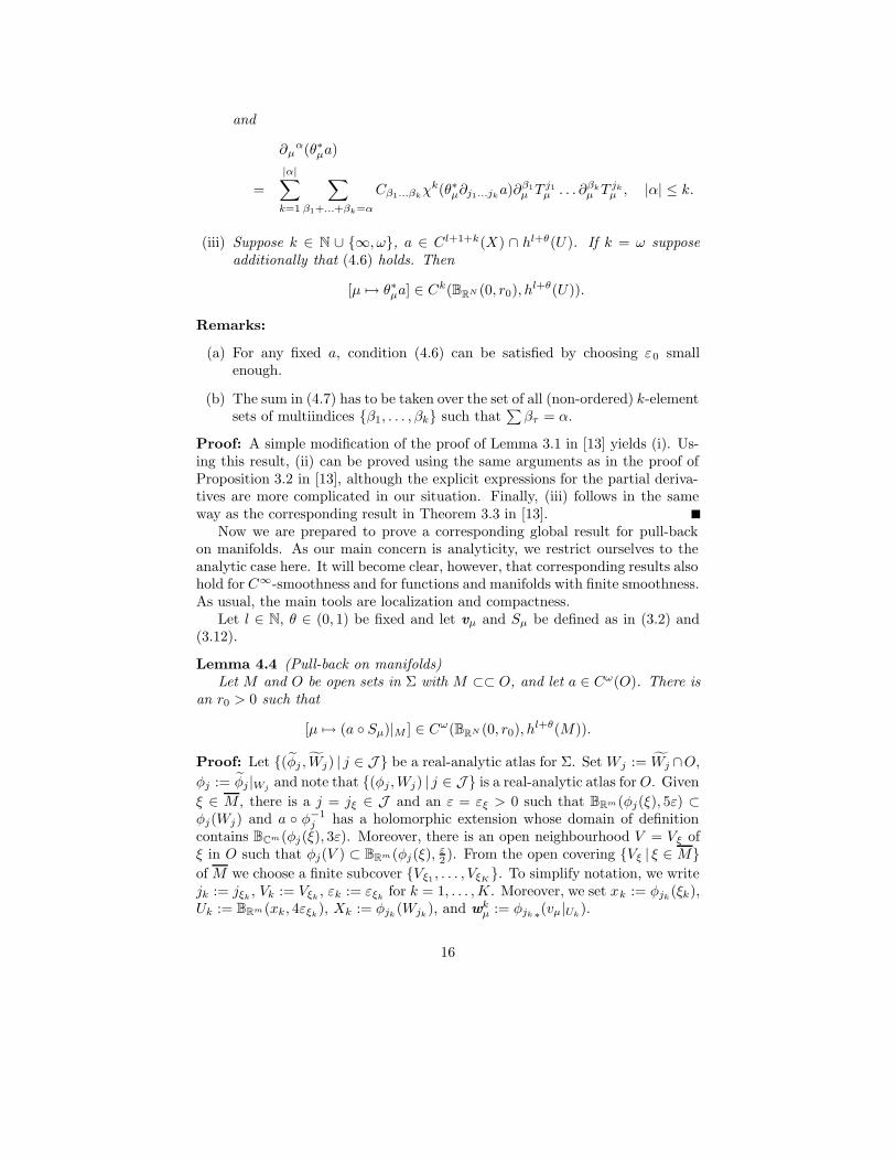
∂µα(θ∗µa)

=

|α|∑

k=1

∑

β1+...+βk=α

Cβ1...βkχk(θ∗µ∂j1...jk

a)∂β1

µ T j1µ . . . ∂βk

µ T jkµ , |α| ≤ k.

(iii) Suppose k ∈ N ∪ ∞, ω, a ∈ Cl+1+k(X) ∩ hl+θ(U). If k = ω supposeadditionally that (4.6) holds. Then

[µ 7→ θ∗µa] ∈ Ck(BRN (0, r0), hl+θ(U)).

Remarks:

(a) For any fixed a, condition (4.6) can be satisfied by choosing ε0 smallenough.

(b) The sum in (4.7) has to be taken over the set of all (non-ordered) k-elementsets of multiindices β1, . . . , βk such that

∑βτ = α.

Proof: A simple modification of the proof of Lemma 3.1 in [13] yields (i). Us-ing this result, (ii) can be proved using the same arguments as in the proof ofProposition 3.2 in [13], although the explicit expressions for the partial deriva-tives are more complicated in our situation. Finally, (iii) follows in the sameway as the corresponding result in Theorem 3.3 in [13].

Now we are prepared to prove a corresponding global result for pull-backon manifolds. As our main concern is analyticity, we restrict ourselves to theanalytic case here. It will become clear, however, that corresponding results alsohold for C∞-smoothness and for functions and manifolds with finite smoothness.As usual, the main tools are localization and compactness.

Let l ∈ N, θ ∈ (0, 1) be fixed and let vµ and Sµ be defined as in (3.2) and(3.12).

Lemma 4.4 (Pull-back on manifolds)Let M and O be open sets in Σ with M ⊂⊂ O, and let a ∈ Cω(O). There is

an r0 > 0 such that

[µ 7→ (a Sµ)|M ] ∈ Cω(BRN (0, r0), hl+θ(M)).

Proof: Let (φj , Wj) | j ∈ J be a real-analytic atlas for Σ. Set Wj := Wj ∩O,

φj := φj |Wjand note that (φj ,Wj) | j ∈ J is a real-analytic atlas for O. Given

ξ ∈ M , there is a j = jξ ∈ J and an ε = εξ > 0 such that BRm(φj(ξ), 5ε) ⊂φj(Wj) and a φ−1

j has a holomorphic extension whose domain of definitioncontains BCm(φj(ξ), 3ε). Moreover, there is an open neighbourhood V = Vξ ofξ in O such that φj(V ) ⊂ BRm(φj(ξ),

ε2 ). From the open covering Vξ | ξ ∈ M

of M we choose a finite subcover Vξ1, . . . , VξK

. To simplify notation, we writejk := jξk

, Vk := Vξk, εk := εξk

for k = 1, . . . ,K. Moreover, we set xk := φjk(ξk),

Uk := BRm(xk, 4εξk), Xk := φjk

(Wjk), and w

kµ := φjk∗(vµ|Uk

).

16

In this setting, we construct T kµ and θk

µ from xk, εk, wkµ in the same way as

Tµ and θµ have been constructed from x0, ε0, wµ in (4.1)–(4.3). There is ansk > 0 such that |µ| < sk implies T k

µ (BRm(xk,εk

2 )) ⊂ BRm(xk, εk). This ensuresthat

θkµ = T k

µ = φjk (Sµ|φ−1

jk(BRm (xk,

εk2

))) φ−1jk, |µ| < sk, (4.7)

on BRm(xk,εk

2 ). Moreover, let πk ∈ C∞0 (Xk) be such that πk ≡ 1 on Uk. For

b ∈ hl+θ(Uk), define Tk(b) := ((πkb) φjk)|M and note that

Tk ∈ L(hl+θ(Uk), hl+θ(M)). (4.8)

We have a φ−1jk

∈ Cω(Xk) ∩ hk,θ(Uk) and therefore, by Lemma 4.3 (iii),

[µ 7→ θkµ

∗(a φ−1

jk)] ∈ Cω(BRN (0, rk), hl+θ(Uk)) (4.9)

for some rk > 0. Set r0 := minrk, sk | k = 1, . . . ,K.Let ψ0, ψ1, . . . , ψK be a partition of unity for Σ subordinate to the open

covering Σ\M,V1, . . . , VK. In particular,∑K

k=1 ψk ≡ 1 on M . Using (4.7)and (4.9) we get by multiplication with ψk φ−1

jk

[µ 7→ (ψk(a Sµ)) φ−1jk

] ∈ Cω(BRN (0, r0), hl+θ(Uk)), (4.10)

k = 1, . . . ,K. Finally,

Tk((ψk(a Sµ)) φ−1jk

) = ψk(a Sµ)|M

and (4.8) yield

[µ 7→ (ψk(a Sµ))|M ] ∈ Cω(BRN (0, r0), hl+θ(M)),

and the lemma follows by summation over k.Remarks:

(a) As Σ is compact, the case M = O = Σ is covered in the above lemma.

(b) The lemma continues to hold if Σ is noncompact. In particular, we canset Σ = Rm.

5 Stokes flow driven by surface tension

In the remaining part of this paper we discuss an application of the abstractresult to a parabolic moving boundary problem from fluid mechanics. Thisapplication is nontrivial in the sense that the evolution equation describing theproblem is nonlocal and the underlying manifold is not assumed to be diffeomor-phic to a symmetric space, hence the results of [13] and [12] are not applicablehere.

Our problem models the creeping flow of a capillary liquid drop and hasthe following exact description (in normalized form): Given a (bounded) initial

17

domain Ω∗ ⊂ Rm+1, we are looking for a family of domains Ω(t) ⊂ Rm+1,parametrized by time t ≥ 0 such that Ω(0) = Ω∗, and t 7→ Γ(t) := ∂Ω(t) is amoving hypersurface such that

Vn(t) = U(·, t)|Γ(t) · ν(t). (5.1)

Here Vn(t) denotes the normal velocity of Γ(t), ν(t) is the outer unit normalvector field on Γ(t) and U(·, t) ∈ C2(Ω(t),Rm+1) is the velocity field of Stokesflow driven by surface tension on Ω(t), i.e. the first component in the solution(U(·, t),Π(·, t)) of

−∆U(·, t) + ∇Π(·, t) = 0 in Ω(t),divU(·, t) = 0 in Ω(t),

T (U(·, t),Π(·, t))ν(t) = κν(t) on Γ(t),

(5.2)

t ≥ 0. Here κ(t) denotes the (m-fold) mean curvature of Γ(t) with the signchosen such that κ(t) is negative if Ω(t) is convex, and T (U,Π) denotes thestress tensor whose cartesian coordinates are

Tij(U,Π) := ∂iUj + ∂jUi − δijΠ.

To enforce uniqueness, (5.2) has to be augmented by the auxiliary conditions

∫

Ω(t)

U(x, t) dx = 0,

∫

Ω(t)

(∂iUj − ∂jUi)(x, t) dx = 0, 1 ≤ i, j ≤ m+ 1, (5.3)

t ≥ 0. (The solvability of (5.2), (5.3) for fixed t in appropriate function spaceswill be addressed below.)

Short-time existence and uniqueness results for (5.1)–(5.3) holding in arbi-trary spatial dimensions are given in [16] and [22], in [16] it is also shown thatthe free boundary is C∞-smooth for all positive times for which the solutionexists, even if Γ(0) has finite smoothness only. For m = 1, see also [5, 6, 14, 20].In these papers, analyticity of the free boundary is proved under the assumptionthat Γ(0) is analytic. Our method enables us to prove analyticity of Γ(t) fort > 0 jointly in space and time under the assumption Γ(0) ∈ h3+θ.

To reformulate our moving boundary problem as an evolution equation on afixed manifold, let Σ be compact closed embedded real-analytic hypersurface inRm+1 near Γ(0) which bounds the bounded domain Ω. We fix θ ∈ (0, 1). Givenk ∈ N, the norm of the space hk+θ(Σ) will be denoted by ‖ · ‖k+θ. Let n denotethe normal field on Σ (exterior to Ω), let U ⊂ Rm+1 be an open neighbourhoodof Σ and let δ > 0 be such that X ∈ Diffω(Σ × (−δ, δ),U) with

X(ξ, ρ) = ξ + ρn(ξ).

Let X−1 := (Ξ, d). Then ∇d(x) = n(Ξ(x)).

18

Suppose r ∈ h2+θ(Σ) is sufficiently small. Then we define

Γr := X(ξ, r(ξ)) | ξ ∈ Σ.

This is an embedded hypersurface in Rm+1 which bounds a bounded domainΩr. To describe the moving boundary we use a mapping [t 7→ r(t)], t ∈ [0, T ],taking small values in h2+θ(Σ), such that Γ(t) = Γr(t), and derive a (nonlocal)evolution equation for r. To simplify notation, we will write r(t, ξ) instead ofr(t)(ξ) for t ∈ [0, T ], ξ ∈ Σ.

Let [t 7→ x(t) := X(ξ(t), r(t, ξ(t)))] be the path of a ”particle” on the movingboundary in Rm+1. Then x(t) = U(x(t), t). This implies (5.1), and we have, inlocal coordinates,

ξα(t) = ∂iΞα(X(ξ, r(t, ξ)))U i(X(ξ, r(t, ξ)), t),

∂tr(t, ξ) + ∂αrξα(t) = ni(ξ)U

i(X(ξ, r(t, ξ)), t),

Hence, suppressing the time argument and setting ψr := Ξ(·, r(·)) we get

∂tr = −P (r) = (ni − ∂αr((∂iΞα) ψr))(U

i ψr). (5.4)

This is the nonlinear evolution equation to which we will apply our abstractresult.

Our next aim is to show assumption (A5) for the operator P . Pick a mapping

S having properties (3.3)–(3.6) and define Sµ according to (3.12). Let D be anopen neighbourhood of 0 in h2+θ(Σ) which is small enough to ensure that P

is well defined on D. Set D := D ∩ h3+θ(Σ). There are neighbourhoods D0

and D0 of 0 in h2+θ(Σ) and h3+θ(Σ), respectively, and an r0 > 0 such that

D0 ⊂ D0, Sµ∗ v ∈ D for all (µ, v) ∈ BRN (0, r0) × D0, and Sµ

∗w ∈ D for all

(µ,w) ∈ BRN (0, r0) × D0. (In the sequel, r0, D0, and D0 will be diminishedwhen necessary without explicit mentioning.)

For (µ,w) ∈ BRN (0, r0) ×D0, let Q(µ,w) be defined by (3.14) with P from(5.4). Then, setting r := Sµ

∗w, using that this implies

∂αw = S∗µ∂βr∂αS

βµ ,

and introducing

φµ,w := ψr Sµ = X(Sµ(·, w(·)) = Sµ + w(n Sµ),

we obtain

Q(µ,w) = P (r) Sµ = ((∂αr Sµ)(∂iΞα φµ,w) − ni Sµ)U i φµ,w

= (∂βw([∂γSδµ]−1)β

α(∂iΞα φµ,w) − ni Sµ)U i φµ,w. (5.5)

Due to (3.3) and Lemma 4.4 we have

[µ 7→ n Sµ] ∈ Cω(BRN (0, r0), (h3+θ(Σ))m+1). (5.6)

19

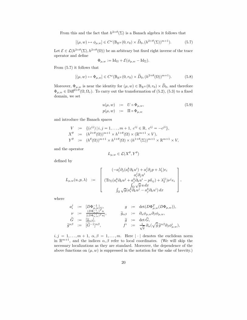
From this and the fact that h2+θ(Σ) is a Banach algebra it follows that

[(µ,w) 7→ φµ,w] ∈ Cω(BRN (0, r0) × D0, (h2+θ(Σ))m+1). (5.7)

Let E ∈ L(h2+θ(Σ), h2+θ(Ω)) be an arbitrary but fixed right inverse of the traceoperator and define

Φµ,w := IdΩ + E(φµ,w − IdΣ).

From (5.7) it follows that

[(µ,w) 7→ Φµ,w] ∈ Cω(BRN (0, r0) × D0, (h2+θ(Ω))m+1). (5.8)

Moreover, Φµ,w is near the identity for (µ,w) ∈ BRN (0, r0) × D0, and therefore

Φµ,w ∈ Diff2+θ(Ω,Ωr). To carry out the transformation of (5.2), (5.3) to a fixeddomain, we set

u(µ,w) := U Φµ,w, (5.9)

p(µ,w) := Π Φµ,w

and introduce the Banach spaces

V := (cij) | i, j = 1, . . . ,m+ 1, cij ∈ R, cij = −cji,Xθ := (h2+θ(Ω))m+1 × h1+θ(Ω) × (Rm+1 × V ),

Y θ := (hθ(Ω))m+1 × h1+θ(Ω) × (h1+θ(Σ))m+1 × Rm+1 × V,

and the operatorLµ,w ∈ L(Xθ, Y θ)

defined by

Lµ,w(u, p, λ) :=

(−ajl ∂j(a

kl ∂ku

i) + aji∂jp+ λi

1)ei

aji∂ju

i

(TrΣ(aki ∂ku

j + akj ∂ku

i − pδij) + λij2 )νjei∫

Ω

√g u dx∫

Ω

√g(ak

i ∂kuj − ak

j ∂kui) dx

,

where

aji := [DΦ−1

µ,w]ij , g := det(DΦTµ,w(DΦµ,w)),

ν :=(DΦ−1

µ,w)T n

|(DΦ−1µ,w)T n|

, gαβ := ∂αφµ,w∂βφµ,w,

G := [gαβ ], g := det G,

gαβ := [G−1]αβ , f i := 1√g∂α(

√g gαβ∂βφ

iµ,w),

i, j = 1, . . . ,m + 1, α, β = 1, . . . ,m. Here | · | denotes the euclidean normin Rm+1, and the indices α, β refer to local coordinates. (We will skip thenecessary localizations as they are standard. Moreover, the dependence of theabove functions on (µ,w) is suppressed in the notation for the sake of brevity.)

20

Pulling back our boundary value problem from Ω(t) = Ωr to Ω via Φµ,w

shows that (5.2), (5.3) is equivalent to

Lµ,w(u(µ,w), p(µ,w), 0) = (0, 0, f, 0, 0),

f := f iei. Here we have used the well-known fact that on an embedded Rieman-nian hypersurface Γ with the metric induced by the ambient space and normalvector n, the curvature vector κn is given by

κn = ∆Γx (5.10)

where ∆Γ is the Laplace-Beltrami operator on Γ and x denotes the embedding ofΓ into the ambient space. The space V is a finite dimensional space of auxiliaryparameters which are necessary to enforce bijectivity of Lµ,w.

Lemma 5.1 We have

aji , g,

√g ∈ Cω(BRN (0, r0) × D0, h

1+θ(Ω)),

ν ∈ Cω(BRN (0, r0) × D0, (h1+θ(Σ))m+1),

gαβ, g,√g gαβ ∈ Cω(BRN (0, r0) ×D0, h

2+θ(Σ)),

f ∈ Cω(BRN (0, r0) ×D0, (h1+θ(Σ))m+1).

Proof: From (5.8) we get

[(µ,w) 7→ DΦ(µ,w)] ∈ Cω(BRN (0, r0) ×D0, h1+θ(Ω)(m+1)×(m+1)). (5.11)

The arguments given in the sequel are based on the fact that the spaces hk+θ(Ω),hk+θ(Σ) are Banach algebras with respect to pointwise multiplication for k ∈ N.This will be used without explicit mentioning. The assertion on g is implied by(5.11), and the assertion on

√g follows from this and the fact that the square

root is an analytic map on the open set

h1+θ+ (Ω) := v ∈ h1+θ(Ω) | v > 0

This can be proved, for example, using the analytic version of the Implicit Func-tion Theorem. As DΦ0,0 = I , we get the assertion on aj

i from the analyticity ofmatrix inversion. Noting additionally that (DΦµ,w)−1)Tn does not vanish, weobtain the assertion on ν i from the analyticity of the map z 7→ 1

|z| from

v ∈ h1+θ(Σ) | v(x) 6= 0 ∀x ∈ Σ

to h1+θ(Σ).Using (5.6), we get, parallel to (5.7),

[(µ,w) 7→ φµ,w] ∈ Cω(BRN (0, r0) ×D0, (h3+θ(Σ))m+1),

and the remaining assertions of the lemma follow from this by arguments anal-ogous to the ones given above.

21

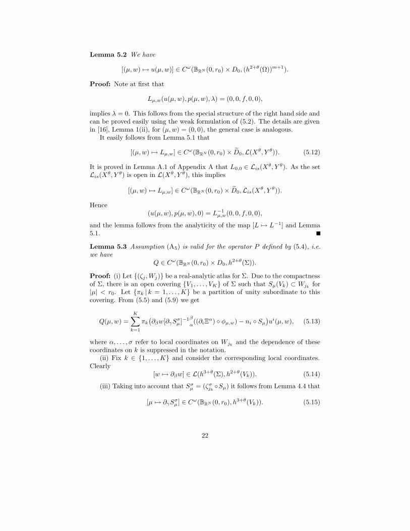
Lemma 5.2 We have

[(µ,w) 7→ u(µ,w)] ∈ Cω(BRN (0, r0) ×D0, (h2+θ(Ω))m+1).

Proof: Note at first that

Lµ,w(u(µ,w), p(µ,w), λ) = (0, 0, f, 0, 0),

implies λ = 0. This follows from the special structure of the right hand side andcan be proved easily using the weak formulation of (5.2). The details are givenin [16], Lemma 1(ii), for (µ,w) = (0, 0), the general case is analogous.

It easily follows from Lemma 5.1 that

[(µ,w) 7→ Lµ,w] ∈ Cω(BRN (0, r0) × D0,L(Xθ, Y θ)). (5.12)

It is proved in Lemma A.1 of Appendix A that L0,0 ∈ Lis(Xθ, Y θ). As the set

Lis(Xθ, Y θ) is open in L(Xθ, Y θ), this implies

[(µ,w) 7→ Lµ,w] ∈ Cω(BRN (0, r0) × D0,Lis(Xθ, Y θ)).

Hence(u(µ,w), p(µ,w), 0) = L−1

µ,w(0, 0, f, 0, 0),

and the lemma follows from the analyticity of the map [L 7→ L−1] and Lemma5.1.

Lemma 5.3 Assumption (A5) is valid for the operator P defined by (5.4), i.e.we have

Q ∈ Cω(BRN (0, r0) ×D0, h2+θ(Σ)).

Proof: (i) Let (ζj ,Wj) be a real-analytic atlas for Σ. Due to the compactnessof Σ, there is an open covering V1, . . . , VK of Σ such that Sµ(Vk) ⊂ Wjk

for|µ| < r0. Let πk | k = 1, . . . ,K be a partition of unity subordinate to thiscovering. From (5.5) and (5.9) we get

Q(µ,w) =

K∑

k=1

πk

(∂βw[∂γS

σµ ]−1β

α((∂iΞ

α) φµ,w) − ni Sµ

)ui(µ,w), (5.13)

where α, . . . , σ refer to local coordinates on Wjkand the dependence of these

coordinates on k is suppressed in the notation.(ii) Fix k ∈ 1, . . . ,K and consider the corresponding local coordinates.

Clearly[w 7→ ∂βw] ∈ L(h3+θ(Σ), h2+θ(Vk)). (5.14)

(iii) Taking into account that Sσµ = (ζσ

jkSµ) it follows from Lemma 4.4 that

[µ 7→ ∂γSσµ ] ∈ Cω(BRN (0, r0), h

3+θ(Vk)). (5.15)

22

Recall that ∂γSσ0 = δσ

γ . Hence the matrix [∂γSσµ ] is invertible in the Banach

algebra (h3+θ(Vk))m×m for small µ, and by the analyticity of matrix inversion,

[µ 7→ [∂γSσµ ]−1] ∈ Cω(BRN (0, r0), (h

3+θ(Vk))m×m). (5.16)

(iv) From Ξ ψr = IdΣ it follows that Ξ φµ,w = Sµ. Differentiating thisidentity with respect to the spatial coordinates and with respect to w yields, inlocal coordinates,

∂βφiµ,w(∂iΞ

α) φµ,w = ∂βSαµ , β = 1, . . .m,

(ni Sµ)(∂iΞα) φµ,w = 0

where α = 1, . . . ,m. For any fixed α, these equations constitute a regular linearsystem of equations for (∂iΞ

α) φµ,w, i = 1 . . .m+ 1, provided (µ,w) is small.Again, by the analyticity of matrix inversion and (5.15),

[(µ,w) 7→ (∂iΞα) φµ,w ] ∈ Cω(BRN (0, r0) ×D0, h

3+θ(Σ)). (5.17)

The assertion of the lemma follows now from (5.6), Lemma 5.2, (5.13),(5.14),(5.16), and (5.17).

Due toP (r) = Q(0, r) = (∂αr(∂iΞ

α φ0,r − ni)ui(0, r),

Lemma 5.3 implies P ∈ Cω(D0, h2+θ(Σ)). Our next aim is to determine the

Frechet derivative ∂P (0) and to show that it generates an analytic semigroupon h2+θ(Σ). From Lemma 5.2 and (5.17) we get

[r 7→ ∂iΞα φ0,r] ∈ Cω(D0, h

3+θ(Σ)),

u(0, ·) ∈ Cω(D0, (h2+θ(Ω))m+1).

Suppressing the fixed argument µ = 0 and writing Π1 for the canonical projec-tion from Xθ onto (h2+θ(Ω))m+1, we get from this

∂P (0)[h] = −ni∂ui(0)[h] + ∂αh∂iΞ

αui(0)

= −n · Π1(L−10 (0, 0, ∂f(0)[h], 0, 0)− L−1

0 ∂L0[h](u(0), p(0), 0))

+∂αh∂iΞαui(0). (5.18)

It remains to calculate ∂f(0)[h]. Using (5.10) and the well-known formula

κ = gαβ∂αβφkrν

k

we getf = gαβ∂αβφ

krν

kν.

The Frechet derivatives of νk, g, and gαβ at r = 0 are given simply by first-orderdifferential operators with smooth coefficients, hence

∂f(0)[h] = gαβ(0)∂αβhhnkn+R1h = ∆Σ(hknk)n+R2h

23

where R1, R2 are given by first-order differential operators with smooth coef-ficients and the gαβ(0) are the contravariant coefficients of the metric on Σinduced from the ambient space.

Consequently, from this and (5.18) we have

∂P (0) = A+B +R3 (5.19)

where

A = n · Π1L−10 (0, 0,−∆Σ(h · n)n, 0, 0),

R3 = n · Π1L−10 ((0, 0,−R2h, 0, 0) + ∂L0[h](u(0), p(0), 0)),

and B is a first-order differential operator with smooth coefficients. From (5.12)and Lemma A.1 it follows that

R3 ∈ L(h2+θ(Σ)). (5.20)

The operator A involves the solution of a BVP for the Stokes equations.Instead of proving a generation result for A + B directly, we will identify Aas a small perturbation of the well-known Dirichlet-Neumann operator for theLaplacian for which generation results are more easily available. To be pre-cise, recall the standard result on the Dirichlet problem for the Laplacian, cf.Theorem B.1,

(∆,TrΣ) ∈ Lis(h3+θ(Ω), h1+θ(Ω) × h3+θ(Σ))

and defineA0 := ∂n(∆,TrΣ)−1(0, ·).

Lemma 5.4 We have

A− 1

2A0 ∈ L(h3+θ(Σ)).

Proof: For h ∈ h3+θ(Σ), let ψ be defined by

ψ := (∆,TrΣ)−1(0, h · n).

Then

L0(∇ψ, 0, 0) = (0, 0, 2(∂2nψ + P(∂ijψnjei)),

∫

Ω

∇ψ dx, 0)

where P denotes the orthogonal projection from Rm+1 onto TΣ again. Defining(v, q, λ) by

L0(v, q, λ) = (0, 0,−2∆Σ(h · n)n, 0, 0)

and using the identity

(∆ψ)|Σ = ∆Σ(ψ|Σ) + ∂2nψ + κ∂nψ

24

we get from Lemmas A.1 and A.2

‖(A0 − 2A)h‖3+θ = ‖(∇ψ − v) · n‖3+θ

= ‖n · Π1L−10 (0, 0, 2(∆Σ(ψ|Σ) + ∂2

nψ + P(∂ijψnjei)),

∫

Ω

∇ψ dx, 0)‖3+θ

≤ 2‖n · Π1L−10 (0, 0,P(∂ijψnjei), 0, 0)‖3+θ

+C‖(0, 0,−2κ∂nψ,

∫

Σ

ψ · n dx, 0)‖Y1+θ

≤ C‖ψ‖3+θ ≤ C‖h‖3+θ.

Together with the fact that both A and A0 map smooth functions to smoothfunctions, this implies the lemma.

Now we are able to prove that P satisfies the crucial assumption on theparabolic character of the evolution problem.

Lemma 5.5 The operator P defined by (5.4) satisfies

∂P (r) ∈ H(h3+θ(Σ), h2+θ(Σ)), r ∈ D0.

Proof: As H(h3+θ(Σ), h2+θ(Σ)) is open in L(h3+θ(Σ), h2+θ(Σ)), it is sufficientto show ∂P (0) ∈ H(h3+θ(Σ), h2+θ(Σ)). We have, according to (5.19),

∂P (0) =1

2(A0 + 2B) + (A− 1

2A0) +R3.

It is shown in Appendix B that A0 +2B ∈ H(h3+θ(Σ), h2+θ(Σ)). Fix θ′ ∈ (0, θ),and ε > 0. Using Lemma 5.4 with θ replaced by θ ′ and the fact that the littleHolder spaces are stable under continuous interpolation, cf. Remark 2.2 f), weget

‖(A− 1

2A0)h‖2+θ ≤ ‖(A− 1

2A0)h‖3+θ′ ≤ ‖h‖3+θ′ ≤ ε‖h‖3+θ + Cε‖h‖2+θ

for any h ∈ h3+θ(Σ) with Cε independent of h. Together with (5.20), thisimplies the lemma by a well-known perturbation result on generators of analyticsemigroups.Remark: Actually, we even have A− 1

2A0 ∈ L(h2+θ(Σ)) and hence it is possibleto have ε = 0 in the last inequality. A proof for this, however, would be moretechnical, an we do not need this result for our present purposes.

Settingr(p, t) := (r(t))(p), p ∈ Σ,

we can prove now our final result on Stokes flow driven by surface tension:

Theorem 5.6 For arbitrary r0 ∈ D0, there is a t+ = t+(r0) > 0 such that theinitial value problem

∂tr + P (r) = 0,r(0) = r0

(5.21)

25

has a unique maximal solution

r = r(·, r0) ∈ C([0, t+), D0) ∩ C1([0, t+), h2+θ(Σ))

andr|Σ×(0,t+) ∈ Cω(Σ × (0, t+)).

Proof: Existence and uniqueness of the solution to (5.21) follow from Lemma5.5, Remark 2.2 j), and Theorem 2.1. It is easy to check that Assumptions(A1)–(A4) hold for the function spaces E0 = h2+θ(Σ) and E1 = h3+θ(Σ) andany family S of mappings satisfying (3.3)–(3.6). Finally, Lemma 5.3 shows thevalidity of Assumption (A5). Thus, our analyticity result follows from Theorem3.9.

Appendices

In the following we prove two results for the BVP (5.2), (5.3) on a fixed domainand a perturbation result for the Dirichlet-Neumann operator which were usedin Section 5, but may be of interest in their own right.

Throughout these appendices, let Ω denote a bounded domain in Rm+1 withsmooth boundary Σ. Given s ≥ 0, we write ‖ · ‖s,Ω and ‖ · ‖s for the norm ofthe spaces hs(Ω) and hs(Σ), respectively. Furthermore, we fix θ ∈ (0, 1).

A The Stokes problem with traction boundary

conditions in little Holder spaces

In this appendix we first establish a regularity result in little Holder spaces in aform suitable for our purposes. Secondly, a sharper estimate is proved which canbe interpreted in the following way: Note that (5.2) is a Neumann problem asthe traction boundary condition (5.2)3 is the natural boundary condition for theStokes operator. The estimate we are going to prove is a consequence of the factthat the ”Neumann-to-Dirichlet operator” belonging to the Stokes equationshas diagonal structure in highest order with respect to the decomposition intotangential and normal components at the boundary. This means, in particular,that the operator mapping the tangential component of the Neumann data tothe normal component of the velocity field at the boundary is of order −2 whilethe full operator has order −1 only. We will prove this using an auxiliary BVPfor the Laplacian.

Recall that we have set

V := (cij) | i, j = 1, . . . ,m+ 1, cij ∈ R, cij = −cji,Xθ := (h2+θ(Ω))m+1 × h1+θ(Ω) × (Rm+1 × V ),

Y θ := (hθ(Ω))m+1 × h1+θ(Ω) × (h1+θ(Σ))m+1 × Rm+1 × V.

26

We further define L := L0,0 ∈ L(Xθ, Yθ) by

L(u, p, λ) =

−∆u+ ∇p+ λ1

divu

T (u, p)n+ λij2 njei∫

Ω u dx∫Ω(∂iu

j − ∂jui) dx

.

Lemma A.1 We haveL ∈ Lis(Xθ, Yθ).

Proof: Let

VR = v ∈ (C∞(Ω))m+1 | vi(x) = sijxj + ci,

sij , ci ∈ R, sij = −sji, i, j = 1, . . . ,m+ 1

be the space of velocity fields belonging to the rigid body motions. Define themappings φ1 and φ2, valued in Rm+1 and V , respectively, by

φ1 : v 7→∫

Ω

v dx,

φij2 : v 7→ 1

2

∫

Σ

(vinj − vjni) dΣ =1

2

∫

Ω

(∂jvi − ∂iv

j) dx

and note that (φ1, φ2) is bijective from VR onto Rm+1 ×V . Choose wj , zij ∈ VR

such that

φj1(wk) = δjk, φij

2 (zkl) = δikδjl, φ1(zkl) = 0, φ2(wk) = 0.

Assume L(u, p, λ) = (f, g, h,M1,M2), λ = (λ1, λ2). The integral identity

1

2

∫

Ω

(∂iuj + ∂ju

i)(∂ivj + ∂jv

i) dx−∫

Ω

p div v dx

=

∫

Ω

(−∆u+ ∇p−∇divu) · v dx+

∫

Σ

T (u, p)n · v dΣ, (A.1)

valid for arbitrary u, v ∈ (h2+θ(Ω))m+1, p ∈ h1+θ(Ω) then implies

λj1 =

∫

Ω

(f −∇g) · wj dx+

∫

Σ

h · wj dΣ,

λij2 =

∫

Ω

(f −∇g) · zij dx+

∫

Σ

h · zij dΣ.

Consequently,|λ| ≤ C(‖f‖θ,Ω + ‖g‖1+θ,Ω + ‖h‖1+θ). (A.2)

In particular, L(u, p, λ) = 0 implies λ = 0 and by (A.1) with v = u also∂iu

j + ∂jui = 0, i.e. u ∈ VR. This yields u = 0 because of

∫Ω u dx = 0,∫

Ω(∂iu

j − ∂jui) dx = 0. Consequently, also p = 0. Hence, L is injective.

27

To show surjectivity, fix (f, g, h,M1,M2) ∈ Yθ and approximate f , g, and hby sequences of smooth functions fk, gk, and hk, respectively, in thenorms of the corresponding spaces. It follows from [16], Lemma 2(i), andthe Sobolev imbedding theorem that there are (uk, pk, λk) ∈ (C∞(Ω))m+1 ×C∞(Ω) × (Rm+1 × V ) such that

L(uk, pk, λk) = (fk, gk, hk,M1,M2). (A.3)

We recall that the Stokes equations form an elliptic system in the sense ofDouglis-Nirenberg and the boundary operator (u, p) 7→ T (u, p)n satisfies thecomplementing boundary condition. Consequently, we have an a priori estimate(cf. [1])

‖uk − ul‖2+θ,Ω + ‖pk − pl‖1+θ,Ω

≤ C(‖fk − fl − ((λk)1 − (λl)1)‖θ,Ω + ‖gk − gl‖1+θ,Ω

+‖hk − hl − ((λk)ij2 − (λl)

ij2 )njei‖1+θ

+‖uk − ul‖L2(Ω)m+1 + ‖pk − pl‖L2(Ω)

).

From a discussion of the weak formulation of (A.3) it follows that

‖uk − ul‖H1(Ω)m+1 + ‖pk − pl‖L2(Ω)

≤ C(‖fk − fl‖((H1(Ω))m+1)′ + ‖gk − gl‖L2(Ω) + ‖hk − hl‖

H12 (Ω)m+1

).

Together with an estimate for λk − λl parallel to (A.2) this yields

‖uk − ul‖2+θ,Ω + ‖pk − pl‖1+θ,Ω

≤ C(‖fk − fl‖θ,Ω + ‖gk − gl‖1+θ,Ω + ‖hk − hl‖1+θ

),

and the surjectivity follows by a standard approximation argument.Remark: A very similar result is stated in [22], Proposition 2.

Lemma A.2 Suppose h ∈ (h1+θ(Σ))m+1 with h · n = 0 and

(u, p, λ) = L−1(0, 0, h, 0, 0). (A.4)

Then u · n ∈ h3+θ(Σ), and there is a constant C independent of h such that

‖u · n‖3+θ ≤ C‖h‖1+θ.

Proof: In the sequel, we will write ∂n = ni∂i for the normal derivative at theboundary. Fix a function d ∈ BUC∞(Ω) with the properties

d|Σ = 0, (∇d)|Σ = n, ∂n(∇d) = 0.

Such a function can easily be constructed by using the signed distance functionnear Σ and cutting it off at large distance from Σ. Extend the normal vectorfield into Ω by setting n = ∇d there.

28

Note that∆p = div(∆u− λ1) = 0 in Ω, (A.5)

and, due to the assumptions on h and the extension of n,

T (u, p)n · n = 2ninj∂iuj − p = 2nj∂nuj − p

= 2∂n(u · n) − p = −λij2 ninj on Σ. (A.6)

Set nowψ := u · n− d

p

2.

Then, because of (A.4) and (A.5),

∆ψ = (∇p− λ1) · n+ 2∂iuj∂inj + u · ∆n− p

2∆d−∇d∇p

= −λ1 · n+ 2∂iuj∂inj + u · ∆n− p

2∆d

and on Σ, due to (A.6),

∂nψ = ∂n(u · n) − p

2= −1

2λij

2 ninj .

A standard a priori estimate for the Laplacian with Neumann boundary datain Holder spaces and Lemma A.1 yield

‖u · n‖3+θ ≤ ‖ψ‖3+θ,Ω ≤ C(‖∆ψ‖1+θ,Ω + ‖∂nψ‖2+θ + ‖ψ‖1+θ,Ω

)

≤ C(‖u‖2+θ,Ω + ‖p‖1+θ,Ω + |λ|Rm+1×V

)≤ C‖h‖1+θ.

B A perturbation result for the Dirichlet-Neu-

mann operator

It is known that the negative Dirichlet-Neumann operator is an elliptic pseudo-differential operator of first order which generates a strongly continuous analyticsemigroup on suitable Holder spaces. We show in this appendix that this gener-ation property is stable under additive perturbations by first order differentialoperators. Note that we do not assume any condition on the L∞-bound of thecoefficients of the perturbation. This means that the general perturbation re-sults for generators of analytic semigroups are not applicable in our setting.

We assume that we are given

ajk, aj , a0 ∈ C∞(Ω), 1 ≤ j, k ≤ m+ 1, b0 ∈ C∞(Σ),

and that there is a positive constant c such that

ajk(x)ξjξk ≥ c|ξ|2, x ∈ Ω, ξ ∈ Rm+1.

29

Given u ∈ h2+θ(Ω), let

Au := −ajk∂j∂ku+ aj∂ju+ a0u, Bu := ajk(TrΣ∂ju)νk + b0TrΣu,

where ν = (ν1, . . . , νm+1) stands for the outer unit normal on Σ and where TrΣ

denotes the trace operator with respect to Σ, i.e. TrΣu = u|Σ is the restictionof u ∈ C1(Ω) to Σ. For simplicity we assume that a0 ≥ 0. It will become clearlater that this is without loss of generality for our purposes, see Theorem B.1.Let (f, g) ∈ hθ(Ω) × h2+θ(Σ) be given. Then it is well-known that there existsa unique classical solution the following BVP

Au = f in Ω, TrΣu = g on Σ. (B.1)

It can be shown that this solution belongs to h2+θ(Ω), see Theorem B.1 below.Let

T := (A, TrΣ)−1∣∣(0 × h2+θ(Σ)

)∈ L(h2+θ(Σ), h2+θ(Ω))

denote the corresponding solution operator with f = 0. Then we call BT theDirichlet-Neumann operator on Σ. It is not difficult to see that

BT ∈ L(h2+θ(Σ), h1+θ(Σ)).

Let now X be a smooth vector field on Σ and define V ∈ L(h2+θ(Σ), h1+θ(Σ))by

Vh := dh(X) for h ∈ h2+θ(Σ).

Observe thatVh = LXh = Xh = (∇Σh|X),

where LX stands for the Lie derivative of h with respect to X .

We next fix l ∈ N with l ≥ 1 and set

E0 := hl+θ(Σ), E1 := hl+1+θ(Σ).

Let L : dom(L) ⊂ h1+θ(Σ) → h1+θ(Σ) be a linear operator. We define theE0-realization LE0

of L to be the linear operator in E0, given by dom(LE0) :=

u ∈ dom(L) ∩ E0 ; Lu ∈ E0 and LE0u = Lu for u ∈ dom(LE0

). Using thisnotation we define

A := E0 − realization of BT , V := E0 − realization of V .

In order to provide a detailed study of the operator A we need the followingadaption of the well-known Agmon-Douglis-Nirenberg a priori estimate:

Theorem B.1 There are λ0 ≥ 0 and µ0 > 0 such that, given λ ≥ λ0 andµ ≥ µ0, we have

(λ+ A,TrΣ) ∈ Lis(hl+1+θ(Ω), hl−1+θ(Ω) × hl+1+θ(Σ)),

(λ+ A, µTrΣ + B) ∈ Lis(hl+1+θ(Ω), hl−1+θ(Ω) × hl+θ(Σ)).

30

Moreover, given λ1 ≥ λ0, there is a positive constant C such that

‖u‖l+1+θ,Ω ≤ C(‖(λ+ A)u‖l−1+θ,Ω + ‖TrΣu‖l+1+θ)

for all u ∈ hl+1+θ(Ω) and all λ ∈ [0, λ1].

Theorem B.1 was shown in [9] in the case l = 1 and for a particular BVP (A, B)on an unbounded domain. The proof there is based on the classical Agmon-Douglis-Nirenberg estimates in Holder spaces, the maximum principle, and thecontinuity method. A careful inspection of that proof shows that it carries overto our situation here. Some arguments are even easier, since we consider here aBVP with smooth coefficients on a bounded domain.

Based on Theorem B.1 we can show the following mapping properties of A:

Lemma B.2 (i) E1 = dom(A), E1 ⊂ dom(V ), and A, V ∈ L(E1, E0).

(ii) µ+A ∈ Lis(E1, E0), provided µ ≥ µ0.

Proof: (i) It follows from Theorem B.1 that E1 = hl+1+θ(Ω) belongs to thedomain of A and that A ∈ L(E1, E0). To verify that dom(A) is contained in E1,let g ∈ dom(A) be given. By construction we have that h := µ0g + BT g ∈ E0

and that v := T g is a solution to

Av = 0 in Ω, (µ0TrΣ + B)v = µ0g + BT g = h on Σ.

Hence Theorem B.1 implies that v ∈ hl+1+θ(Ω) and therefore g = v|Σ ∈hl+1+θ(Σ) = E1. The assertion for V is clear.

(ii) Let µ ≥ µ0 and assume that g ∈ E1 satisfies (µ+A)g = 0. Writing v := T g,we have

Av = 0 in Ω, (µTrΣ + B)v = µg + BT g = 0 on Σ.

Thus Theorem B.1 implies that g = 0. Let now f ∈ E0 be given. Then TheoremB.1 ensures that there is a v ∈ hl+1+θ(Ω) such that

Av = 0 in Ω, (µTrΣ + B)v = f on Σ.

This yields

T TrΣv = (A,TrΣ)−1(0,TrΣv) = (A,TrΣ)−1(A,TrΣ)v = v.

Putting now g := TrΣv, we conclude that g ∈ E1 and that

(µ+A)g = (µ+ BT )g = (µTrΣ + B)v = f.

Hence (i) and the open mapping theorem imply the assertion. This completesthe proof.

Remark: Assume that X(p) 6= 0 for all p ∈ Σ. Then one can show thatdom(V ) = E1 if and only if m = 1. We omit a proof of this assertion, since we

31

shall not need this property of V in the following.

Let now (U,ϕ) be a local chart of Ω such that U ∩ Σ 6= ∅. We may assumethat the corresponding parameter domain ϕ(U) is given by B := Bm+1∩ Hm+1

+ ,

where Hm+1+ := x ∈ Rm+1, xm+1 ≥ 0 denotes the ”positive half space” in

Bm+1 with respect the (m + 1)-th co-ordinate. The local representations of(A, B, V) are denoted by (A, B, V). This means that

Aϕ∗ = ϕ∗A, Bϕ∗ = ϕ∗B, Vϕ∗ = ϕ∗V .

It is well-known that there are

ajk, aj , a0, bj ∈ BUC∞(B), 1 ≤ j, k ≤ m+ 1,

b0, cα ∈ BUC∞(B ∩ (Rm × 0)), 1 ≤ α ≤ m,

such that

[ajk(x)] is symmetric and positive definite, bn(x) > 0, (B.2)

for all x ∈ B, and such that

A = −ajk∂j∂k + aj∂j + a0, B = −bj∂j + b0, V = cα∂α.

Let now

ajk0 := ajk(0), bj0 := bj(0), cα0 := cα0 (0), 1 ≤ j, k ≤ m+ 1, 1 ≤ α ≤ m.

Furthermore, we introduce

~a := (a1(m+1)0 , . . . , a

m(m+1)0 ), e0 := a

(m+1)(m+1)0 , d0(ξ) := aαβ

0 ξαξβ ,

where ξ ∈ Rm, and define the following parameter-dependent quadratic poly-nomial:

qξ(z) := 1 + d0(ξ) + 2i(~a|ξ)z − e0z2, z ∈ C.

It follows from the fact that the matrix [ajk0 ] is positive definite that, given

ξ ∈ Rm, there exists exactly one root λ(ξ) of qξ(·) with positive real part, whichis given by

λ(ξ) =i(~a|ξ)e0

+1

e0

√e0(1 + d0(ξ)) − (~a|ξ)2.

This root is now used to introduce the following Fourier multiplication operator,acting on functions defined on Rm. Given g ∈ hl+1+θ(Rm), let

T0g(x, y) := [F−1e−λ(·)yFg](x), (x, y) ∈ Rm × R+,

where F denotes the Fourier transform on Rm. Finally, we define the followingoperators

Gt := B0T0 + tV0, t ∈ [0, 1], (B.3)

32

where B0 := −bj0∂j and V0 := cα0 ∂α, and the function

gt(ξ) := bm+10 λ(ξ) − i(~b+ t~c|ξ), ξ ∈ Rm, t ∈ [0, 1],

where ~b := (b10, . . . , bm0 ) and ~c := (c10, . . . , c

m0 ). Then one shows as in Lemma 4.1

in [11] that Gt is a Fourier multiplication operator with symbol gt, i.e. we have

Gt = F−1gtF , t ∈ [0, 1]. (B.4)

Based on (B.4), we now obtain as in [11, Theorem 4.2]:

Theorem B.3 Gt ∈ H(hl+1+θ(Rm), hl+θ(Rm)), t ∈ [0, 1].

Setting Gt := A + tV for t ∈ [0, 1], we are prepared to prove for the followinggeneration result:

Theorem B.4 Gt ∈ H(E1, E0), t ∈ [0, 1].

Proof: (i) We first introduce an equivalent norm on hl+k+θ(Σ), k ∈ 0, 1,which will be useful in what follows. In order to do so, we note that there exists afinite family of charts (Ur, ϕr) ; 1 ≤ r ≤ N such that Ur∩Σ, ϕr |(Ur∩Σ) ; 1 ≤r ≤ N is an atlas for Σ. Further, there exist test functions ψr ∈ D(Ur) suchthat ψr ; 1 ≤ r ≤ N is a partition of unity on a compact neighbourhood of Σin ∪N

r=1Ur. Finally, in the following we write ‖ · ‖s,Rm for the norm in hs(Rm),s > 0. It is known that

[h 7→ max1≤r≤N

‖(ϕr)∗(ψrh)‖l+k+θ,Rm ] (B.5)

defines an equivalent norm on hl+k+θ(Σ) for k ∈ 0, 1, see [23].

(ii) Given r ∈ 1, . . . , N, we obtain a family of operators G rt ; t ∈ [0, 1] of the

form (B.3), using the above construction on the chart (Ur, ϕr). In the followingwe suppress the index r ∈ 1, . . . , N. Clearly, we can and will choose theconstants in the estimates below to be independent of r. Invoking TheoremB.3, we know that there are positive constants C1 and λ1 such that

‖g‖l+1+θ,Rm + |λ|‖g‖l+θ,Rm ≤ C1‖(λ+ Gt)g‖l+θ,Rm (B.6)

for all g ∈ hl+1+θ(Rm), λ ∈ [Re z ≥ λ1], and t ∈ [0, 1].

(iii) Fix σ ∈ (0, θ). Shrinking the diameter of the chart domain U , we mayassume that there exists a positive constant C2 such that

‖ϕ∗(ψGth) − Gtϕ∗(ψh)‖l+θ,Rm ≤ 1

2C1‖ϕ∗(ψh)‖l+1+θ,Rm + C2‖h‖l+1+σ (B.7)

for all h ∈ hl+1+θ(Σ). The proof of (B.7) is based on the fact that T0 canbe interpreted as the solution operator of the elliptic BVP on the half spaceHm+1

+ , which arises from the original BVP given by (A, B) after flattening the

33

boundary, freezing the coefficients, and considering top order terms only. Forthe details we refer to [11, Lemma 5.1]. Combining (B.6) and (B.7), we get

‖ϕ∗(ψh)‖l+1+θ,Rm + |λ|‖ϕ∗(ψh)‖l+θ,Rm

≤ 2C1‖ϕ∗(ψ(λ +Gt)h)‖l+θ,Rm + C2‖h‖l+1+σ(B.8)

for all h ∈ hl+1+θ(Σ), λ ∈ [Re z ≥ λ1], and t ∈ [0, 1]. Using the norm given in(B.5), we find a positive constant C such that

‖h‖l+1+θ + |λ|‖h‖l+θ ≤ C

2‖(λ+Gt)h‖l+θ + C‖h‖l+1+σ (B.9)

for all h ∈ hl+1+θ(Σ), λ ∈ [Re z ≥ λ1], and t ∈ [0, 1].

(iv) We next absorb the second term on the right-hand side of (B.9) into theleft-hand side of (B.9). For this recall that

hl+1+σ(Σ) = (hl+θ(Σ), hl+1+θ(Σ))01−θ+σ,∞,

see Remark 2.2 f). Using the corresponding interpolation inequality, it followsfrom Young’s inequality that there is a positive constant C3 such that

‖h‖l+1+σ ≤ 1

2C‖h‖l+1+θ + C3‖h‖l+θ, h ∈ hl+1+θ(Σ). (B.10)

Combining (B.9) and (B.10), we find

‖h‖l+1+θ + |λ|‖h‖l+θ ≤ C‖(λ+Gt)h‖l+θ (B.11)

for all ∈ hl+1+θ(Σ), λ ∈ [Re z ≥ λ∗], and t ∈ [0, 1], where λ∗ := 2 maxλ1, CC3.

(v) It follows from (B.11), Lemma B.4(ii), and a well-known homotopy argu-ment, cf. [15, Theorem 5.2], that there is a λ0 > 0 such that

λ0 +Gt ∈ Lis(hl+1+θ(Σ), hl+θ(Σ)), t ∈ [0, 1]. (B.12)

Now the assertion follows from (B.11), (B.12) and Remark 2.2 h).

References

[1] Agmon, S., Douglis, A., Nirenberg, L.: Estimates near the boundary forsolutions of elliptic partial differential equations satisfying general boundary con-ditions II; Comm. Pure Appl. Math. 17 (1964) 35–92.

[2] Amann, H.: Linear and Quasilinear Parabolic Problems, Vol. I, Birkhauser, 1995.

[3] Angenent, S.: Nonlinear analytic semiflows. Proc. Roy. Soc. Edinburgh 115A

(1990), 91–107.

[4] Angenent, S.: Parabolic equations for curves on surfaces, Part I. Curves withp-integrable curvature. Annals of Math. 132 (1990) 451–483.

34

[5] Antanovskii, L.K.: Analyticity of a free boundary in plane quasi-steady flowof a liquid form subject to variable surface tension, in: Proc. of Conference: TheNavier-Stokes Equations II: Theory and Numerical Methods, Oberwolfach 1991,Springer 1993, 1–16.

[6] Antanovskii, L.K.: Creeping thermocapillary motion of a two-dimensional de-formable bubble: existence theorem and numerical simulation, Eur. J. Mech.,B/Fluids 11 (1992) 6 741–758.

[7] Baillon, J. B.: Caractere borne de certains generateurs de semigroup lineairedans les espaces de Banach, C.R. Acad. Sc. Paris 290 A (1980), 757–760.

[8] Da Prato, G., Grisvard, P.: Equations d’evolution abstraites nonlineaires detype parabolique, Ann. Mat. Pura Appl. 120 (1979), 329–396.

[9] Escher, J., Simonett, G.: Maximal regularity for a free boundary problem,NoDEA 2 (1995), 463–510.

[10] Escher, J., Simonett, G.: Analyticity of the interface in a free boundaryproblem, Math. Ann. 305 (1996), 439–459.

[11] Escher, J., Simonett, G.: Classical solutions of multidimensional Hele-Shawmodels, SIAM J. Math. Anal. 28 (1997), 1028–1047.

[12] Escher, J., Simonett, G.: Analyticity of solutions to fully nonlinear parabolicevolution equations on symmetric spaces, to appear.

[13] Escher, J., Pruß, J., Simonett, G.: A new approach to the regularity ofsolutions for parabolic equations, to appear.

[14] Friedman, A., Reitich, F.: Quasistatic motion of a capillary drop. I. Thetwo-dimensional case, J. Diff. Eq. 178 (2002) 212–263.

[15] Gilbarg, D., Trudinger, N. S.: Elliptic Partial Differential Equations of Sec-ond Order, Springer, 1977.

[16] Gunther, M., Prokert, G.: Existence results for the quasistationary motion ofa capillary liquid drop, Zeitschrift fur Analysis und ihre Anwendungen 16 (1997)2 311–348.

[17] Hirsch, M.W.: Differential Topology, Springer 1997.

[18] Lunardi, A.: Analytic Semigroups and Optimal Regularity in Parabolic Equa-tions. Birkhauser, Basel, 1991.

[19] Pazy, A. Semigroups of Linear Operators and Applications to Partial DifferentialEquations, Springer 1983.

[20] Prokert, G.: On the existence of solutions in plane quasistationary Stokes flowdriven by surface tension, Euro. Journ. of Appl. Math. 6 (1995) 539–558.

[21] Simonett, G.: Center manifolds for quasilinear reaction-diffusion systems, Dif-ferential Integral Equations 8 (1995), 753–796.

35

[22] Solonnikov, V.A.: On quasistationary approximation in the problem of mo-tion of a capillary drop, in: Escher, J., Simonett, G. (Eds.):Topics in nonlinearanalysis, Birkhauser 1999, 643–671.

[23] Triebel, H.: Theory of Function Spaces, Birkhauser, Basel, 1983.

[24] Triebel, H.: Theory of Function Spaces II, Birkhauser, Basel, 1992.

Joachim Escher

Institute of Applied Mathematics, University of Hannover, Welfengarten 1, 30167 Han-nover, Germany

e-mail: escher@ifam.uni-hannover.de

Georg Prokert

Faculty of Mathematics and Computing Science, Technical University Eindhoven, POBox 513, 5600 MB Eindhoven, The Netherlands

e-mail: g.prokert@tue.nl

36