Analytical-Numerical Solution of a Parabolic Diﬀusion ...¬€usion equations arise in many...

Ingeniería y CienciaISSN:1794-9165 | ISSN-e: 2256-4314ing. cienc., vol. 11, no. 22, pp. 49–72, julio-diciembre. 2015.http://www.eafit.edu.co/ingcienciaThis article is licensed under a Creative Commons Attribution 4.0 by

Analytical-Numerical Solution of a

Parabolic Diffusion Equation Under

Uncertainty Conditions Using DTM with

Monte Carlo Simulations

Gilberto González-Parra1, Abraham J. Arenas2 and Miladys Cogollo 3

Received: 09-02-2015 | Accepted: 18-06-2015 | Online: 31-07-2015

MSC: 35K10, 65C05, 65M99, 35R60

doi:10.17230/ingciencia.11.22.3

Abstract

A numerical method to solve a general random linear parabolic equationwhere the diffusion coefficient, source term, boundary and initial condi-tions include uncertainty, is developed. Diffusion equations arise in manyfields of science and engineering, and, in many cases, there are uncertaintiesdue to data that cannot be known, or due to errors in measurements andintrinsic variability. In order to model these uncertainties the correspon-ding parameters, diffusion coefficient, source term, boundary and initialconditions, are assumed to be random variables with certain probabilitydistributions functions. The proposed method includes finite differenceschemes on the space variable and the differential transformation methodfor the time. In addition, the Monte Carlo method is used to deal withthe random variables. The accuracy of the hybrid method is investigatednumerically using the closed form solution of the deterministic associated

1 Universidad de Los Andes, Mérida, Venezuela, [email protected] Universidad de Córdoba Montería, Colombia, [email protected] Universidad EAFIT, Medellín, Colombia, [email protected] .

Universidad EAFIT 49|

http://www.eafit.edu.co/ingciencia/

http://orcid.org/0000-0001-5847-678X

http://orcid.org/0000-0003-3106-1271

http://orcid.org/0000-0002-6583-4693

mailto:[email protected]



Analytical-Numerical Solution of a Parabolic Diffusion Equation Under Uncertainty

Conditions Using DTM with Monte Carlo Simulations

equation. Based on the numerical results, confidence intervals and ex-pected mean values for the solution are obtained. Furthermore, with theproposed hybrid method numerical-analytical solutions are obtained.

Key words: random linear diffusion models; uncertainty conditions; fi-nite difference schemes; differential transformation method; analytical-numerical solution

Solución numérico-analítica de una ecuación dedifusión bajo condiciones de incertidumbreutilizando DTM y Monte Carlo

ResumenUn método numérico para resolver una ecuación parabólica general aleato-ria lineal donde el coeficiente de difusión, el término fuente, las condicionesde contorno e iniciales incluyen la incertidumbre, se ha desarrollado. Ecua-ciones de difusión surgen en muchos campos de la ciencia y la ingeniería,y en muchos casos, existen la incertidumbres debido a los datos que no sepueden saber, o debido a errores en las mediciones y la variabilidad intrín-seca. Para modelar estas incertidumbres los parámetros correspondientes,coeficiente de difusión, término fuente, condiciones de contorno e iniciales,se suponen que son variables aleatorias con determinadas distribucionesde probabilidad. Basándose en los resultados numéricos, se obtienen losintervalos de confianza y valores medios esperados para la solución. Ade-más, se obtienen con las soluciones numéricas-analíticas del método híbridopropuesto.

Palabras clave: modelos lineales de difusión aleatorios; condiciones de

incertidumbre; Esquemas de diferencias finitas; método de transformación

diferencial; solución analítica-numérica

1 Introduction

Differential equations, in general, describe the rate of change in the physi-cal property of matter with respect to time and/or space. Real phenomenalead to complicated differential equations, which seldom have exact solu-tions. The difficulty of obtaining analytical solutions and the availabilityof fast computing power make numerical techniques attractive. However,numerical methods can have slow convergence and instability problems.

Mathematical models dealing with uncertainty in differential equationshave been considered in recent decades in a wide variety of applied areas,

|50 Ingeniería y Ciencia

G. González, A. J. Arenas and M. Cogollo

such as physics, chemistry, biology, economics, sociology and medicine.Differential deterministic equations have been extensively studied, bothfrom both analytical and numerical viewpoints. However, in many situ-ations, equations with random inputs are better suited in describing thereal behavior of quantities of interest than their counterpart deterministicequations. Randomness in the input may arise because of errors in theobserved or measured data, variability in experiment and empirical condi-tions, uncertainties (variables that cannot be measured or missing data) orplainly because of lack of knowledge [1],[2].

Differential equations where some or all the coefficients are consideredrandom variables or that incorporate stochastic effects (usually in the formof white noise) have been increasingly used in the last few decades to dealwith errors and uncertainty and represent a growing field of great scientificinterest [3],[4],[5],[6]. Additionally, uncertainty can be considered on the ini-tial conditions or source term. Applications of the aforementioned randomdifferential equations are wave propagations in homogeneous media, sys-tems and structures with parametric excitations, dynamics of imperfectlyknown systems in physics, epidemics, medicine and biology [7],[8],[4].

Analytical treatment of random differential equations has been done by[4]. It is important to remark that in general the statistical moments suchas mean and variance of the solution process cannot be determined easily,see [4, Ch. 6] for details. Several applications to real world problems thatconsider randomness or uncertainty have been developed [9],[10],[11]

The present work combines finite difference schemes for the discretiza-tion space with the differential transformation method for the time dis-cretization. In addition, randomness is introduced in the diffusion PDE

which models several physical processes and to the best of our knowledgethis whole process has not be done before. The differential transformationmethod has been applied in several works and recently has been extendedsuccessfully to random differential equations [12],[13]. The randomness isincorporated since inaccuracies in the physical measurements can affectseveral inputs of the diffusion PDE such as diffusion coefficient, sourceterm, boundary and initial conditions, and can thus introduce some degreeof uncertainty. In real world applications, the probability density functionsof those quantities can only be estimated from physical measurements. Itis important to remark that even if these measurements are done with the

ing.cienc., vol. 11, no. 22, pp. 49–72, julio-diciembre. 2015. 51|



utmost care, the measured values will differ somewhat and some statisticaltests are necessary to find the probability density distributions of thesemeasurements.

The most commonly used distribution is the Gaussian one [1]. However,other distributions such as Uniform, Beta and Gamma are also used andmay be more appropriate if enough data points are available to suggestthose distributions.

The real world is much more complex than anything that can be createdwith arithmetic and logical operations [14, p.341 and p.342]. Therefore itis necessary to use methods that include some real world complexity likerandomness [15]. The Monte Carlo method is one of the most versatileand widely used numerical methods to deal with randomness. The powerof Monte Carlo simulation modeling allows us to include more complexityto the deterministic mathematical model by incorporating the impact ofrandomness on the dependent variables [16]. Random effects and the va-riations produced by using different probability distributions can be studiedusing Monte Carlo simulations. Applications of the Monte Carlo methodin different areas are given, for example, in [17],[18],[11].

The Monte Carlo method is used here with the aim of obtaining quali-tative and quantitative behavior of the numerical solutions of the randomdiffusion PDE. The Monte Carlo simulation differs from traditional simu-lation in that the model input parameters are treated as random variables,rather than as fixed values. These parameters must be identified with theiruncertainty ranges and shapes of their probability density functions pres-cribed. There are no restrictions on the shapes of the probability densityfunctions, although most studies make use of the basic ones, such as nor-mal, log-normal, uniform, or triangular. Maximum and minimum limits oneach input parameter can be prescribed to prevent unrealistic selection ofextreme values [19].

The main reason here to apply the Monte Carlo method is due to thesimplicity and effectiveness with which it deal with random variables. Themajor challenge with the method is to efficiently carry out many realizationsand then to summarize the results into a few useful values such as theexpectation and higher moments of the solution stochastic processes [20].The Monte Carlo method for solving random differential equations can be



described briefly as:

• Generate sample values of the random input from their known orassumed probability density function.

• Solve the deterministic equation corresponding to each value.

• Calculate statistics, such as mean and variance, of the set of deter-ministic solutions.

The number of realizations or runs can be as large as desired. However,there is always a compromise that must be reached concerning the optimalnumber of runs, since each run takes a certain time on the computer. Diffe-rent criteria can be used to choose the number of realizations and this is nota straightforward task. A useful criteria on to select the optimal numberof realizations is to stop when the increasing them does not significantlychange expected value and variance of the physical process solution. Othercriteria include theoretical ones using Central Limit Theorem, t-Student

distribution and other probabilistic tools. Finally, it is important to remarkthat the numerical simulation time can be easily reduced using parallelprocesses.

The paper is organized as follows. In Section 2 the diffusion PDE ispresented. Section 3 is devoted to present the basic properties of the diffe-rential transformation method. Numerical results for the deterministic andrandom PDE, including studies of the accuracy, are presented in Section4. Finally, in Section 5 discussion and conclusions are presented.

2 Diffusion differential equation

In this paper, we consider a general random linear parabolic equation wherethe diffusion coefficient, source term, boundary and initial conditions in-clude uncertainty. The deterministic associated problem is the followingparabolic equation:

ut(x, t) = [p(x, t)ux(x, t)]x + f(x, t), 0 < x < 1, t > 0, (1i)

u(0, t) = g1(t), t > 0, (1ii)




u(1, t) = g2(t), t > 0, (1iii)

u(x, 0) = g(x), 0 ≤ x ≤ 1. (1iv)

Physically speaking, this model describes the heat conduction proce-dure in a given inhomogeneous medium with some input heat source f(x, t).The coefficient p(x, t) represents heat conduction property namely the heatcapacity. The type of boundary condition used occurs when the ends ofthe bar are at given temperatures.

In a limited set of cases, solutions can be obtained in closed form byseparation of variables. Thus, the great importance of numerical methodsto calculate approximate solutions. Numerical approximations should pre-serve the dynamical behavior of the exact solution of the model and careshould be used to avoid spurious solutions and instabilities. It is well knownthat the relation ∆t

∆x2 , where ∆t is the time step and ∆x the spatial gridsize, is critical for the numerical stability of the explicit finite differenceschemes for this class of PDE, which puts serious restrictions on the timestep. Therefore it is necessary to develop schemes that are robust with athreshold of convergence greater than for the traditional schemes.

In this paper, we introduce a hybrid method that combines the finitedifference numerical schemes and an analytic-numerical method, the diffe-rential transformation method, to solve the diffusion PDE (1i)-(1iv) withrandomness. The differential transformation technique is used to transformthe governing equations from the time domain into the spectrum domain,followed by use of the finite difference method to formulate discretized ite-ration equations appropriate for rapid computation. Unlike the traditionalhigh-order Taylor series method, which requires a many symbolic com-putations, the present method involves simple iterative procedures in thespectrum domain. The approximate solution is then obtained from a thepartial sum of the inverse process.

3 Basic definitions of differential transformation method

Pukhov [21], proposed the concept of differential transformation, where theimage of a transformed function is computed by differential operations. It isdifferent from traditional integral transforms such as Laplace and Fourier.



This method becomes a numerical-analytic technique that formalizes theTaylor series in a totally different manner. The differential transformationis a computational method that can be used to solve linear and non-linearordinary and partial differential equations with their corresponding initialand/or boundary conditions. A pioneer using this method to solve ini-tial value problems is Zhou [22], who introduced it in a study of electricalcircuits. Additionally, the differential transformation method (DTM) hasbeen applied to solve a variety of problems that are modeled with differ-ential equations [23],[24],[25],[26],[27]. Some authors mentioned that DTMcan be seen as computer-specialized procedure to compute the Taylor series[28].

The method consists of, given a system of differential equations andrelated initial conditions, transforming these into a system of recurrenceequations that finally leads to a system of algebraic equations whose solu-tions are the coefficients of a power series solution. The numerical solutionof the system of differential equation in the time domain can be obtainedin the form of a finite-term series in terms of a chosen system of basis func-tions. In this method, we take tk+∞

k=0 as a basis functions and thereforethe solution is obtained in the form of a Taylor series. Other bases may bechosen, see [29]. The advantage of this method is that it is not necessary todo linearization or perturbations. Furthermore, large computational workand round-off errors are avoided. It has been used to solve effectively, easi-ly and accurately a large class of linear and nonlinear problems. However,to the best of our knowledge, the differential transformation has not beenapplied yet in seasonal epidemic models. For the sake of clarity, we presentthe main definitions of the DTM as follows:

Definition 3.1. Let x(t) be analytic in the time domain D, then it hasderivatives of all orders with respect to time t. Let

ϕ(t, k) =dkx(t)

dtk, ∀t ∈ D. (2)

For t = ti, then ϕ(t, k) = ϕ(ti, k), where k belongs to a set of non-negativeintegers, denoted as the K domain. Therefore, (2) can be rewritten as

X(k) = ϕ(ti, k) =

[

dkx(t)

dtk

]

t=ti

(3)




where X(k) is called the spectrum of x(t) at t = ti.

Definition 3.2. Suppose that x(t) is analytic in the time domain D, thenit can be represented as

x(t) =∞∑

k=0

(t− ti)k

k!X(k). (4)

Thus, the equation (4) represents the inverse transformation of X(k).

Definition 3.3. If X(k) is defined as

X(k) = M(k)

[

dkx(t)

dtk

]

t=ti

(5)

where k ∈ Z+ ∪ 0, then the function x(t) can be described as

x(t) =1

q(t)

∞∑

k=0

(t− ti)k

k!

X(k)

M(k), (6)

where M(k) 6= 0 and q(t) 6= 0. M(k) is the weighting factor and q(t) isregarded as a kernel corresponding to x(t).

Note, that if M(k) = 1 and q(t) = 1, then Eqs. (3), (4), (5) and (6)are equivalent.

Definition 3.4. Let [0,H] be the interval of simulation with H the timehorizon of interest. We take a partition of the interval [0,H] as 0 =t0, t1, ... , tn = H such that ti < ti+1 and Hi = ti+1− ti for i = 0, ... , n− 1.

Let M(k) =Hk

i

k! , q(t) = 1 and x(t) be a analytic function in [0,H]. It thendefines the differential transformation as

X(k) =Hk

i

k!

[

dkx(t)

dtk

]

t=ti

where k ∈ Z+ ∪ 0, (7)

and its differential inverse transformation of X(k) is defined as follow

x(t) =∞∑

k=0

(

t

Hi

)k

X(k), for t ∈ [ti, ti+1]. (8)



For the interested readers, the operation properties of the differentialtransformation method can be found in [21],[22].

From the definitions above, we can see that the concept of differentialtransformation is based upon the Taylor series expansion. Note that, theoriginal functions are denoted by lowercase letters and their transformedfunctions are indicated by uppercase letters. Thus, applying the DTM , asystem of differential equations in the domain of interest can be transformedto an algebraic equation system in the K domain and, thus x(t) can beobtained by a finite-term Taylor series plus a remainder, i.e.,

x(t) =1

q(t)

n∑

k=0

(t− ti)k

k!

X(k)

M(k)+Rn+1 =

n∑

k=0

(

t

H

)k

X(k) +Rn+1, (9)

where

Rn+1 =

∞∑

k=n+1

(

t

H

)k

X(k), and Rn+1 → 0 as n → ∞.

In many modeling situations, the computation interval [0,H] is notalways small, and in order to accelerate the rate of convergence and to im-prove the accuracy of the calculations, it is necessary to divide the entiredomain H into n subdomains. This process can be seen as a implementa-tion of an analytic continuation process due to the fact that the range ofconvergence of the direct sum of the series is too limited [28]. Moreover,in this case, the DTM is truly different from the raw Taylor series methodwhich, stricto sensu, does not involve any consideration of analytic conti-nuation [28]. The main advantage of the domain splitting process is thatonly a few Taylor series terms are required to construct the solution in asmall time interval Hi, where H =

∑ni=1Hi. It is important to remark

that, Hi can be chosen arbitrarily small if necessary. Thus, the system ofdifferential equations can be solved in each subdomain [24]. Consideringthe function x(t) in the first sub-domain (0 ≤ t ≤ t1, t0 = 0), the onedimensional differential transformation is given by

x(t) =n∑

k=0

(

t

H0

)k

X0(k) , where X0(0) = x0(0). (10)




Notice that since the series converges in the domain [ti, ti + 1], its sumprovides the solution in this domain with a sensible accuracy. Moreover, ifthis is true for each value ti then one gets, step by step, an approximatesolution in the whole domain [0,H], each initial value x(Hi being (appro-ximately) provided by the sum of the series at the second boundary ofthe preceding sub-domain. Therefore, the differential transformation andsystem dynamic equations can be solved for the first subdomain and X0

can be solved entirely in the first subdomain. The end point of functionx(t) in the first subdomain is x1, and the value of t is H0. Thus, x1(t) isobtained by the differential transformation method as

x1(H0) = x(H0) =

n∑

k=0

X0(k). (11)

Since that x1(H0) represents the initial condition in the second subdomain,then X1(0) = x1(H0). And so the function x(t) can be expressed in thesecond sub-domain as

x2(H1) = x(H1) =n∑

k=0

X1(k). (12)

In general, in each i− 1 subdomain one gets,

xi(Hi) = xi−1(Hi−1)+

n∑

k=1

Xi−1(k) = Xi−1(0)+

n∑

k=1

Xi−1(k), i = 1, 2, ..., n.

(13)Using the D spectra method described above, the function x(t) can beobtained throughout the entire domain.

4 Construction of the hybrid scheme using DTM and finite

differences for reaction-diffusion PDE

Our goal in this section is to construct a hybrid scheme for Eq. (1i) com-bining the DTM and finite differences as follows: we begin taking thedifferential transforms of both sides of the governing equations from the



time domain into the spectrum domain, i.e., taking the differential trans-formation with respect to the time variable t only. Thus, from Eq. (1) onegets the following spectrum:

(k + 1)U(x, k)

Hi

=∂

∂x

( k∑

l=0

P(x, k)∂U(x, k − l)

∂x

)

+F(x, k), 0 < x < 1, k ≥ 0, (14i)

U(0, k) = G1(k), k ≥ 0, (14ii)

U(1, k) = G2(k), k ≥ 0, (14iii)

U(x, 0) = g(x), 0 ≤ x ≤ 1, (14iv)

where U(x, k), G1(k), G2(k) are the differential transform of u(x, t), g1(t),and g2(t), respectively.

The finite difference method is then applied to Eq. (14), which containsonly derivatives with respect to the space coordinates x. The whole domainis divided into M equal subintervals of length ∆x of the interval 0 ≤ x ≤ 1.The x coordinates of the grid points are given by xj = j∆x, for j = 0, ...,M .Using the central difference formula on the first and second derivatives, andthe convolution of transformation in Eq. (14), the corresponding differenceequation is given by

(k + 1)Uj(k)

Hi

=

k∑

l=0

Pj+ 1

2

(k)Uj+1(k − l)

∆x2+

k∑

l=0

(

Pj+ 1

2

(k) +Pj− 1

2

(k)

)

Uj(k − l)

∆x2

+

k∑

l=0

Pj− 1

2

(k)Uj−1(k − l)

∆x2+Fj(k), k ≥ 0.

Thus, we obtain a numerical scheme to compute the coefficients of thepower series to obtain the solution in the respective subinterval, which isgiven by:

Uj(k) =Hi

k + 1

k∑

l=0

Pj+ 1

2

(k)Uj+1(k − l)

(∆x)2+

k∑

l=0

(

Pj+ 1

2

(k) +Pj− 1

2

(k)

)

Uj(k − l)

(∆x)2

+

k∑

l=0

Pj− 1

2

(k)Uj−1(k − l)

(∆x)2+ Fj(k)

k ≥ 0, (15i)




U0(k) =G1(k), k ≥ 0, (15ii)

UM (k) =G2(k), k ≥ 0, (15iii)

Uj(0) =gj , For j = 0, ...,M , (15iv)

where bold uppercase letters are for the transformed functions. Thus, froma process of inverse differential transformation, the solutions on each sub-domain can be obtained using n+ 1 terms for the power series, i.e.,

uj(t) =n∑

k=0

(

t

Hi

)k

Uj(k), 0 ≤ t ≤ Hi, (16)

and then the solution is given by:

u(x, t) =

M−1∑

j=1

uj(t), for 0 < x < 1. (17)

5 Numerical results

In this section, numerical comparisons between the hybrid method and theanalytical solution are presented in order to show the accuracy of the hybridmethod for solving the diffusion PDE. In addition, combining the hybridmethod with the Monte Carlo simulations we investigate the effect of in-troducing randomness on the diffusion coefficient, source term, boundaryand initial conditions. Numerical simulations are performed with differentrealizations, time step sizes and parameters of the probabilistic distribu-tions. The expected solution is computed as the average of several randomsolutions. The numerical results are presented mostly at the value x = 0.5,since this is the middle point of the interval of interest and generally is thepoint where the numerical methods give less accurate results. Graphicalresults corroborate this last fact. The randomness is included assuming auniform probabilistic distribution. However, the methodology it is easilyextendable to other probabilistic distributions. It is important to mentionthat the methodology proposed here is three-folded. The first step is to



obtain the numerical scheme to compute the coefficients of the power se-ries. This step includes to obtain the spectra of the equation consideredand its discretization. In the second step, the numerical solution for eachrealization is computed. Finally, based on the Monte Carlo method manyrealizations are obtained and some statistics regarding the ensemble arecomputed. Therefore, the computation time of the whole process dependson many variables such as, the spectra, time step (for DTM and the finitedifference scheme) and number of realizations. However, it has been men-tioned in other works that the DTM is faster than the multistage Adomianmethod, but the Runke-Kutta methods require less computation time incomparison with DTM and multistage Adomian [12].

Example 5.1. We consider the following deterministic problem

ut(x, t) = [p(x, t)ux(x, t)]x + f(x, t),

u(0, t) = et, 0 < t ≤ 1,

u(1, t) = e1+t, 0 < t ≤ 1,

u(x, 0) = ex, 0 < x < 1,

where u(x, t) is unknowns in (0, 1)×(0, 1], and the terms f(x, t) = ex+t(1−(1 + 0.1xt) − 0.1t) and p(x, t) = 1 + 0.1xt are given. The exact solution isgiven by u(x, t) = ex+t, [30].

We also consider the random version of Example (5.1), by introducingthe following perturbations:

u(x, 0, γ) =ex + γ, (18i)

u(0, t, γ) =et + γ, u(1, t, γ) = e1+t + γ, (18ii)

p(x, t, γ) =1 + 0.1xt + γ, and (18iii)

f(x, t, γ) =− 0.1ex(1 + x)tet + γ, (18iv)

where the unknown u(x, t, γ) as well as u(x, 0, γ), u(0, t, γ), u(1, t, γ), p(x, t, γ),f(x, t, γ), are stochastic processes (s.p.) defined on a common probabilityspace (Ω,F ,P) and γ is the random variable (r.v.), which consists of threecomponents:




1. The sample space Ω which is a non-empty set that collects all theelementary events or states ω.

2. A collection of subsets of Ω called σ-algebra F ( or Borel field) thatsatisfies: the empty set is an element of F , F is closed under com-plementation and under countable unions.

3. A probability function P with domain F , and γ is a random varia-ble (r.v.) defined on the original sample space Ω with probabilityfunction.

A solution of Example (5.1) with randomness means that for each γ ∈ Ω,u(x, t, γ) is a solution of the deterministic problem obtained from Example(5.1) taking realizations of the involved r.v, and where derivatives andlimits are regarded in the mean square sense, see [4] for details. Sincethe solutions are stochastic processes, we can rely on the Monte Carlomethod to compute them. It is important to remark that here we considerrandomness on the initial conditions, diffusion coefficient, source term andboundary conditions separately.

The Monte Carlo method (with Simple Random Sampling) for uncer-tainty analysis is quite simple. At first, the more important inputs have tobe identified as shown in (18). Next, uncertainty ranges and shapes of theirprobability density functions need to be chosen. Here, we choose as a firstapproach to test the methodology with uniform probability density func-tions for each r.v.. Thus, Example (5.1) is solved for each value assigned tothe random variables to obtain results using the probability density func-tion prescribed. The process is repeated many times, with the values ofthe input random parameters chosen from the corresponding distributions,in order to obtain a large ensemble of solutions [19]. In other words, wesample from the probability density function in order to assign that valueto the random variable considered, and solve the Example (5.1) using theDTM for each number sampled. It is important to emphasize that themethod can be used with the input parameters having an arbitrary shapeof probability density function.

In order to compute the coefficients of the power series of the randomsolution in the algebraic system (15) the following spectra are introduced:



Uj(k, γ) =ej∆x + δ(k)γ, (19i)

U0(k, γ) =Hk

i eiHi

k!+ δ(k)γ, UM (k, γ) = eM∆xHk

i eiHi

k!+ δ(k)γ, (19ii)

Pj± 1

2

(k, γ) =δ(k) + 0.1(j ±1

2)∆xδ(k − 1) + δ(k)γ, and (19iii)

Fj(k, γ) =− 0.1(1 + j∆x)ej∆x

k∑

l=0

Hk+1−li eiHi

(k − l)!δ(k − 1) + δ(k)γ, (19iv)

where i denotes the i-th split domain.

5.1 Numerical comparisons in accuracy

In Table 1 we present the absolute errors at x = 0.5 comparing the hy-brid method and the analytical solutions of the deterministic problem ofExample (5.1) when a space step size ∆x = 0.05 is used. The accuracy ofthe DTM hybrid method is improved by using the h-refinement approach(reducing the time step size).

In Table 2 we present the absolute errors at x = 0.5 comparing thehybrid method and the analytical solutions of the deterministic problem ofExample (5.1) using different space step sizes ∆x and a fixed time step size∆t = 0.0001. The accuracy of the DTM hybrid method is improved in thiscase by using the h-refinement approach in the space variable x. However,as it is remarked in [31] high space segmentation may cause divergencephenomenon. On the other hand, the p-refinement approach (increasingthe number of terms) does not increase the accuracy of the hybrid methodfor this specific reaction-diffusion PDE due to its structure.

On the left hand side of Figure 1 it can be seen that the hybrid methodreproduces the correct behavior of the solution for the diffusion PDE. Inaddition, on the right hand side of Figure 1 it can be observed that theabsolute value of the error of the hybrid method increases with time andthe maximum values are around the middle of the interval [0, 1]. Thus, thestudy of the error at x = 0.5 is justified. These results show the numericalconsistency of the hybrid method.




Table 1: Numerical absolute errors using the hybrid method with 3-terms, diffe-rent time step sizes and a space step size ∆x = 0.05 for the deterministic versionof Example (5.1) at x = 0.5

T ime h = 0.001 h = 0.0005

0.1 0.39E − 4 0.52E-50.2 0.58E − 4 0.70E-50.5 0.82E − 4 0.61E-51.0 0.12E − 3 0.31E-52.0 0.24E − 3 0.76E-4

Table 2: Numerical absolute errors using the hybrid method with 3-terms, di-fferent space step sizes and a fixed time step size h = 0.0001 for the deterministicversion of Example (5.1) at x = 0.5

T ime ∆x = 0.05 ∆x = 0.04 ∆x = 0.033

0.1 0.39E − 4 0.11E-4 0.59E-50.2 0.58E − 4 0.17E-4 0.93E-50.5 0.82E − 4 0.29E-4 0.16E-41.0 0.12E − 3 0.56E-4 0.31E-42.0 0.24E − 3 0.18E-3 0.11E-3

Figure 1: Numerical solution for the deterministic version of Example (5.1) using 5 terms

for the DTM with h = 0.001 and ∆x = 0.1 for the finite difference (left). Plotting of the error

for different times and values of the space variable x. (right)



5.2 Randomness on the initial condition

Graphical results of Monte Carlo simulations using 50 realizations for therandom version of Example (5.1) presented in and assuming a uniformprobabilistic distribution for the initial conditions are shown on the lefthand side of Figure 2. It can be observed that the expected solution (i.e.average of the ensemble of the realizations) does not agree with the solutionof the deterministic version Example (5.1). However, it can be seen on theright hand side that when the number of realizations is increased to 200the expected solution agrees very well with the solution of the deterministicversion of Example (5.1).

In addition, it can be seen in Figures 2 and 3 that the amplitude of theconfidence intervals decreases and converges to the expected solution, as weincrease the number of realizations. This fact is of paramount importancefrom a physical point of view since it means that no matter how large isthe error of the initial conditions measure, the solution will approximateasymptotically to the deterministic solution. The right hand side of Figure3 shows the expected solution and confidence intervals when it is assumednormal probabilistic distribution for the initial conditions. Notice thatthe numerical results are similar to the ones with uniform probabilisticdistribution but with less dispersion as was expected from the Gaussianform of the normal distribution.

0 0.02 0.04 0.06 0.08 0.11

1.2

1.4

1.6

1.8

2

2.2

2.4

Time t

u(0

.5,t)

Solution

Expected Solution

95% Confidence Interval

0 0.02 0.04 0.06 0.08 0.10.8

1

1.2

1.4

1.6

1.8

2

2.2

2.4

2.6

Time t

u(0

.5,t)

Solution

Expected Solution


Figure 2: Numerical solution for the random version of Example (5.1) at x = 0.5 assuming

that initial conditions are perturbed by a term that follows a uniform distribution [−1.0, 1.0]

with 50 (left) and 200 (right) realizations. Solutions are computed using 5 terms in the DTM ,

h = 0.0001 and ∆x = 0.1 for the finite difference.




0 0.1 0.2 0.3 0.4 0.51

1.2

1.4

1.6

1.8

2

2.2

2.4

2.6

2.8

Time t

u(0

.5,t)

Solution

Expected Solution


0 0.02 0.04 0.06 0.08 0.11

1.2

1.4

1.6

1.8

2

2.2

2.4

Time t

u(0

.5,t)

Solution

Expected Solution



that initial conditions are perturbed by a term that follows a uniform distribution [−1.0, 1.0](left)

and a normal distribution [0, 1/1.96] (right) with 150 and 200 realizations respectively. Solutions

are computed using 5 terms in the DTM , h = 0.0001 and ∆x = 0.1 for the finite difference.

5.3 Randomness on the boundary condition

In this subsection some Monte Carlo simulations are performed in order toobserve the impact of boundary conditions uncertainties on the solution ofthe random version of Example (5.1).

0 0.2 0.4 0.6 0.8 11.5

2

2.5

3

3.5

4

4.5

5

Time t

u(0

.5,t)

Solution

Expected Solution


0 1 2 3 4 50

50

100

150

200

250

Time t

u(0

.5,t)

Solution

Expected Solution



that boundary conditions are perturbed by a term that follows a uniform distribution [−0.1, 0.1]

with 100(left) and 20(right) realizations. Solutions are computed using 5 terms in the DTM ,

h = 0.0001 and ∆x = 0.1 for the finite difference.



In Figure 4 it can be seen that the expected solution has a similarbehavior as the deterministic solution when a uniform probabilistic distri-bution is used for the boundary conditions. The right hand side of Figure 4shows that the amplitude of the confidence interval does not increase withtime since the variance of the solution is exactly the variance of γ. This isdue to the fact that perturbing the boundary conditions leads to an exactsolution u(x, t) = ex+t + γ.

5.4 Randomness on the source term

In Figure 5 it can be seen that the expected solution agrees with the de-terministic solution when a uniform probabilistic distribution is used forthe source term. Notice that the amplitude of the 95% confidence interval(i.e. he range in which 95% of the realizations are found) increases withtime. Therefore, the uncertainty on the source term is propagated over thetime, giving rise with large probability to unpredictable feasible solutions.This fact is important from the physical point of view since it means thatcareful attention must be paid to the measure or estimation of the sourceterm in order to have realistic solutions.

0 0.02 0.04 0.06 0.08 0.11.6

1.65

1.7

1.75

1.8

1.85

1.9

1.95

Time t

u(0

.5,t)

Solution

Expected Solution



that the source term has in addition an uncertainty term that follows an uniform distribution

[−1.0, 1.0] and performing 100 realizations. It is computed using 5-term in the DTM , h = 0.0001

and ∆x = 0.1 for the finite difference.




5.5 Randomness on the diffusion coefficient

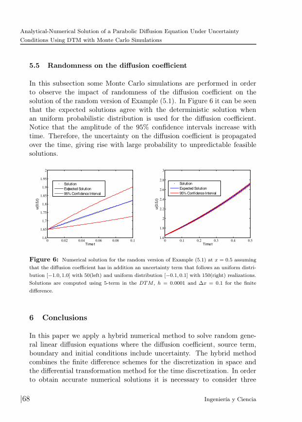
In this subsection some Monte Carlo simulations are performed in orderto observe the impact of randomness of the diffusion coefficient on thesolution of the random version of Example (5.1). In Figure 6 it can be seenthat the expected solutions agree with the deterministic solution whenan uniform probabilistic distribution is used for the diffusion coefficient.Notice that the amplitude of the 95% confidence intervals increase withtime. Therefore, the uncertainty on the diffusion coefficient is propagatedover the time, giving rise with large probability to unpredictable feasiblesolutions.

0 0.02 0.04 0.06 0.08 0.11.6

1.65

1.7

1.75

1.8

1.85

1.9

1.95

2

Time t

u(0

.5,t)

Solution

Exphected Solution


0 0.1 0.2 0.3 0.4 0.51.6

1.8

2

2.2

2.4

2.6

2.8

3

Time t

u(0

.5,t)

Solution

Expected Solution



that the diffusion coefficient has in addition an uncertainty term that follows an uniform distri-

bution [−1.0, 1.0] with 50(left) and uniform distribution [−0.1, 0.1] with 150(right) realizations.

Solutions are computed using 5-term in the DTM , h = 0.0001 and ∆x = 0.1 for the finite

difference.

6 Conclusions

In this paper we apply a hybrid numerical method to solve random gene-ral linear diffusion equations where the diffusion coefficient, source term,boundary and initial conditions include uncertainty. The hybrid methodcombines the finite difference schemes for the discretization in space andthe differential transformation method for the time discretization. In orderto obtain accurate numerical solutions it is necessary to consider three



issues: the first is the time step size used in the differential transformationmethod. The second one is the step size in the space for the finite differencescheme and the last is the order of the differential method. The accuracyof the DTM hybrid method can be improved by using the h-refinementapproach in time and space variables. In addition due to the structureof the considered PDE the p-refinement approach does not improve theaccuracy of the solutions for more than 3-terms. Nevertheless, in generalincreasing the differential transform order gives more accurate solutions atthe expense of more computation time.

The diffusion PDE has been selected due to the fact that reaction-diffusion equations arise in many fields of science and engineering, and, inmany cases, there are uncertainties due to data that cannot be known, ordue to errors in measurements and intrinsic variability. In order to modelthese uncertainties some probability distributions functions are assumedfor the diffusion coefficient, source term, boundary and initial conditions.

The effect of introducing randomness in the diffusion PDE is justifiedby the fact that the diffusion coefficient, source term, boundary and ini-tial conditions have some degree of uncertainty. Therefore, the randomdiffusion PDE is investigated by means of the well known Monte Carlomethod. Based on the numerical results, confidence intervals and expectedmean values for the solution are obtained. These confidence intervals areproportional to the variance of the probabilistic distributions of the ran-dom variable assumed for the diffusion coefficient, source term, boundaryand initial conditions. This means that the dynamics behavior of the di-ffusion physical process can be predicted with some probability despite theuncertainty of the diffusion coefficient, source term, boundary and initialconditions. Finally it is important to mention that Monte Carlo simula-tions give realistic values which are consistent with the results obtained forthe deterministic diffusion PDE. Future works can be developed for morecomplex cases such a nonlinear system with two interacting scalar fields.

Acknowledgements

The authors thank the anonymous reviewers for their helpful suggestionsand remarks. The first author has been partially supported by CDCHTA-ULA project grant I-1289-11-05-A.




References

[1] F. Boano, R. Revelli, and L. Ridolfi, “Stochastic modelling of DO and BODcomponents in a stream with random inputs,” Advances in Water Resources,vol. 29, no. 9, pp. 1341 – 1350, 2006. 51, 52

[2] B. Chen-Charpentier, B. Jensen, and P. Colberg, “Random Coefficient Dif-ferential Models of Growth of Anaerobic Photosynthetic Bacteria,” ETNA,vol. 34, pp. 44–58, 2009. 51

[3] B. Oksendal, Stochastic Differential Equations. Springer, New York, 1995.51

[4] T. Soong, Probabilistic Modeling and Analysis in Science and Engineering.Wiley, New York, 1992. 51, 62

[5] B. M. Chen-Charpentier, J.-C. Cortés, J.-V. Romero, and M.-D. Roselló,“Some recommendations for applying gPC (generalized polynomial chaos)to modeling: An analysis through the Airy random differential equation,”Applied Mathematics and Computation, vol. 219, no. 9, pp. 4208 – 4218,2013. 51

[6] G. González-Parra, B. Chen-Charpentier, and A. J. Arenas, “Polynomialchaos for random fractional order differential equations,” Applied Mathemat-

ics and Computation, vol. 226, pp. 123 – 130, 2014. 51

[7] E. Vanden Eijnden, “Studying random differential equations as a tool forturbulent diffusion,” Phys. Rev. E, vol. 58, no. 5, pp. R5229–R5232, Nov 1998.[Online]. Available: http://link.aps.org/doi/10.1103/PhysRevE.58.R5229 51

[8] B. Kegan and R. West, “Modeling the simple epidemic with deterministicdifferential equations and random initial conditions,” Math. Biosc, vol. 195,pp. 197–193, 2005. 51

[9] H. Kim, Y. Kim, and D. Yoon, “Dependence of polynomial chaos on randomtypes of forces of KdV equations,” Applied Mathematical Modelling, vol. 36,no. 7, pp. 3080 – 3093, 2012. 51

[10] J. Wu, Y. Zhang, L. Chen, and Z. Luo, “A Chebyshev interval method fornonlinear dynamic systems under uncertainty,” Applied Mathematical Mod-

elling, vol. 37, no. 6, pp. 4578 – 4591, 2013. 51

[11] S. Bhatnagar and Karmeshu, “Monte-Carlo estimation of time-dependent sta-tistical characteristics of random dynamical systems,” Applied Mathematical

Modelling, vol. 35, no. 6, pp. 3063 – 3079, 2011. 51, 52


http://link.aps.org/doi/10.1103/PhysRevE.58.R5229


[12] G. Gonzalez-Parra, L. Acedo, and A. Arenas, “Accuracy of analytical-numerical solutions of the Michaelis-Menten equation,” Computational &

Applied Mathematics, vol. 30, no. 2, pp. 445–461, 2011. 51, 61

[13] L. Villafuerte and B. Chen-Charpentier, “A random differential transformmethod: Theory and applications,” Applied Mathematics Letters, vol. 25,no. 10, pp. 1490–1494, 2012. 51

[14] F. Morrison, The Art of Modeling Dynamic Systems. John Wiley, 1991. 52

[15] Y. Chen, J. Liu, and G. Meng, “Incremental harmonic balance method fornonlinear flutter of an airfoil with uncertain-but-bounded parameters,” Ap-

plied Mathematical Modelling, vol. 36, no. 2, pp. 657 – 667, 2012. 52

[16] V. Mallet and B. Sportisse, “Air quality modeling: From deterministic tostochastic approaches,” Comput. Math. Appl, vol. 55, no. 10, pp. 2329–2337,5 2008. 52

[17] S. D. Brown, R. Ratcliff, and P. L. Smith, “Evaluating methods for approx-imating stochastic differential equations,” Journal of Mathematical Psychol-

ogy, vol. 50, no. 4, pp. 402–410, 8 2006. 52

[18] S. Wu, “The Euler scheme for random impulsive differential equations,” Ap-

plied Mathematics and Computation, vol. 191, no. 1, pp. 164–175, 2007. 52

[19] S. R. Hanna, J. C. Chang, and M. E. Fernau, “Monte Carlo estimates ofuncertainties in predictions by a photochemical grid model (uam-iv) due touncertainties in input variables,” Atmospheric Environment, vol. 32, no. 21,pp. 3619–3628, 1998. 52, 62

[20] K. M. Hanson, “A framework for assessing uncertainties in simulation pre-dictions,” Physica D: Nonlinear Phenomena, vol. 133, no. 1-4, pp. 179–188,1999. 52

[21] G. Pukhov, Differential Transformations of Functions and Equations.Naukova Dumka (in Russian), 1980. 54, 57

[22] J. Zhou, Differential Transformation and its Applications for Electrical Cir-

cuits. Huazhong University Press, Wuhan (in Chinese), 1986. 55, 57

[23] J. Biazar and M. Eslami, “Differential transform method for quadratic Riccatidifferential equation,” International Journal of Nonlinear Science, vol. 9,no. 4, pp. 444–447, 2010. 55

[24] A. J. Arenas, G. González-Parra, and B. M. Chen-Charpentier,“Dynamical analysis of the transmission of seasonal diseases usingthe differential transformation method,” Mathematical and Computer

Modelling, vol. 50, no. 5–6, pp. 765 – 776, 2009. [Online]. Available:http://dx.doi.org/10.1016/j.mcm.2009.05.005 55, 57


http://dx.doi.org/10.1016/j.mcm.2009.05.005



[25] I. A.-H. Hassan, “Application to differential transformation method forsolving systems of differential equations,” Applied Mathematical Modelling,vol. 32, pp. 2552–2559, 2008. 55

[26] M. Jang and C. Chen, “Analysis of the response of a strongly nonlineardamped system using a differential transformation technique,” Applied Math-

ematics and Computation, vol. 88, pp. 137–151, 1997. 55

[27] V. S. Ertürk, G. Zaman, and S. Momani, “A numeric–analytic method forapproximating a giving up smoking model containing fractional derivatives,”Computers & Mathematics with Applications, vol. 64, no. 10, pp. 3065–3074,2012. 55

[28] C. Bervillier, “Status of the differential transformation method,” Applied

Mathematics and Computation, vol. 218, no. 20, pp. 10 158 – 10 170, 2012.55, 57

[29] I. Hwang, J. Li, and D. Du, “A numerical algorithm for optimal controlof a class of hybrid systems: differential transformation based approach,”International Journal of Control, vol. 81, no. 2, pp. 277–293, 2008. [Online].Available: http://dx.doi.org/10.1080/00207170701556880 55

[30] C. E. Mejía and D. A. Murio, “Numerical identification of diffusivity coef-ficient and initial condition by discrete mollification,” Comput. Math. Appl,vol. 12, pp. 35–50, 1995. 61

[31] C.-K. Chen and S.-P. Ju, “Application of differential transformation totransient advective-dispersive transport equation,” Applied Mathematics and

Computation, vol. 155, no. 1, pp. 25 – 38, 2004. 63


http://dx.doi.org/10.1080/00207170701556880

Analytical-Numerical Solution of a Parabolic Diﬀusion ...¬€usion equations arise in many...

Documents

Transcript of Analytical-Numerical Solution of a Parabolic Diﬀusion ...¬€usion equations arise in many...