1

ANALYTICAL METHOD FOR THE PREDICTION OF RELIABILITY AND

MAINTAINABILITY BASED LIFE-CYCLE LABOR COSTS

Mark Fitzpatrick

ISDS, Product Support

The Boeing Company

Wichita, KS

Robert Paasch

Department of Mechanical Engineering

Oregon State University

Corvallis, OR

1 INTRODUCTION

In today's competitive marketplace, the quality of a product is becoming increasingly more

important. The informed customer not only weighs the ability of the product to meet his/her

requirements, and the purchase price of the product, but also the money that must be expended to

maintain the function of the product. Hence, lowering the life-cycle cost of a product will increase its

value and attractiveness to the customer.

Reliability and Maintainability greatly influence the life-cycle cost of complex systems. The

more reliable and the more maintainable the product is, the lower its life-cycle cost will be.

Reliability is defined as the probability that an item will adequately perform its specified purpose for a

specified period of time under specified environmental conditions (Leemis, 1995). Maintainability is

defined as the probability that an item will be retained in or restored to a specified condition within a

given period of time (Blanchard, 1995). A Portion of the research in Reliability and Maintainability

(R&M) addresses the importance of accurately quantifying the life-cycle cost of a product and

subsequently lowering that cost. However, most R&M research in this area has not attempted to

utilize R&M analysis as a design tool. The accepted R&M analysis methods are used for the

evaluation of existing products based on test data retrieved from the product. Unfortunately, if the

2

R&M analysis gives evidence for a design change, the implementation of that change would be very

expensive due to the tardiness its implementation.

The objective of this research was to develop an analytical method to adequately determine the

R&M based life-cycle cost of a product early in its design phase, with the ability to compare

competing designs or design changes and show the effects the competing designs or design changes

may have on the life-cycle cost of the product. Early in the design process, information needed to

accurately determine R&M costs will be missing or incomplete and any analysis must be regarded as a

rough estimation. As the design of the product becomes more refined, the predictive accuracy will

increase. The method presented in this paper was developed to aid the designer in optimizing the

operating costs of the product early in the design process instead of making design modifications after

a prototype has been built and tested.

The analytical method that is presented predicts three variables for each component within a

system, Mean Time Between Failure (MTBF), Mean Time Between Unscheduled Removal

(MTBUR), and Mean Time Between Maintenance Actions (MTBMA). Those variables are then used

to find the average Line Labor Cost (LLC) and Shop Labor Cost (SLC) for each component. All the

associated labor costs for the components in the system are summed together to supply the predicted

labor cost for maintaining the system.

The Bleed Air Control System (BACS) from the Boeing 737-300/400/500 was chosen as a test

model for the analysis for several reasons. First, there was very detailed life-cycle data available for

the 737 so a comparison of actual labor cost versus the predicted labor cost could be performed.

Second, there was a complete Failure Modes and Effects Analysis (FMEA) available on the 737

BACS that could be easily converted into a fault tree analysis. Lastly, the BACS has a history of

having high maintenance costs and being misdiagnosed, so there was a corporate interest in finding a

solution to increase the diagnosability and lower the maintenance costs of the BACS.

2 BACKGROUND

Most Reliability and Maintainability (R&M) analytical methods concentrate on utilizing

laboratory test data to provide an adequate estimate of the life-cycle cost of a product. All share a

commonality in that they utilize short time period test data to determine the life-cycle failure data.

3

Ansell (1994) explains and demonstrates a good number of the common reliability data analysis

methods.

Some R&M researchers have concentrated on specialized areas within the whole of Reliability and

Maintainability. A portion of this research is attempting to predict measures that influence the life-

cycle cost of a product prior to attaining test data from a prototype. One method being developed is

Service Mode Analysis (Bryan, 1992). Service modes are the ways in which a system may be serviced

and Service Mode Analysis is a method for describing which service modes will impact a particular

design and in what manner (Gershenson, 1991). This method separates analyzing service modes into

two categories, Component-based service modes and Phenomena based service modes. The superiority

of phenomena based service modes analysis is presented and phenomena based service cost is

expressed as a function of labor time, labor rate, necessary tools, necessary training, replacement part

cost, and replacement part availability. Later research in this area (Eubanks, 1993, Marks, 1993)

progresses the development of a computer software package to perform serviceability analysis. The

computer program operates by defining items and their connection to other items. Each item in a

system can be defined as either a component, subassembly, fastener, or process and its relationship to

other items can be described as covers, attaches to, connects to, engages, or supported by. Repair

operations within the program can be defined as replace, repair, overhaul, adjust/align, or

tighten/connect/lubricate. By assessing all the inputs, a method for analyzing and comparing

competing designs is developed. More recent research (Di Marko, 1995) introduces a computerized

method of performing an initial Failure Modes and Effects Analysis (FMEA), this is combined with

the previous research to increase the predictive ability of Service Mode Analysis. This research is

progressing the predictability of maintainability issues, however, it does not devote the same effort to

predicting reliability related issues or the diagnostic process.

Attention is also being devoted to the diagnosability of a product Research in this area by Ruff

(1997) developed form-to-function mapping. Form-to-function mapping is a method of graphically

representing the relationships between function, performance measures, and components in a

mechanical system. Ruff shows that modifying the interaction between components and performance

measures could increase the diagnosability of the system.

4

Clark (1996) developed a distinguishability metric for the evaluation a competing designs based

on diagnosability. The distinguishability metric is a function of the total number of failure

indications, the total number of components, and the number of candidate components per failure

indication. Clark utilized the Bleed Air Control System (BACS) on the Boeing 747 as a test model

to verify his results.

Wong (1994) attempted to link diagnosability directly with life-cycle-cost. This method utilizes

the probability of a failure indication occurring multiplied by the average time to diagnose the failure

indication and the hourly maintenance cost to yield a cost estimate based on diagnosability. When the

cost to diagnose all the possible failure indications for a system are summed, a life-cycle cost estimate

is arrived at. A similar method is utilized by Goldberg (1987) to determine component reliability of

an electric power feeder.

Murphy (1997) developed a method for determining the Mean Time Between Unscheduled

Removal (MTBUR) of system components. Unscheduled removal of components is separated into

two categories, justified and unjustified. The justified unscheduled removals are equivalent to the

Mean Time Between Failure (MTBF) of the component. An unjustified unscheduled removal is

defined as the unscheduled removal of a component that has not failed. A formula is developed to

determine the unjustified unscheduled removal of components based on the MTBF's of other possible

failed components and the labor involved in component removal.

The largest failing of the for-mentioned diagnosability research, based on predictability, is its

reliance on historical failure data. This research will utilize much that has been previously developed

in diagnosability, but with the addition of a process to predict the required failure data.

3 DESCRIPTION OF THE 737-300/400/500 BLEED AIR CONTROL SYSTEM

Since the 737 BACS is used as a test model to demonstrate the analysis method, it would be

appropriate to introduce the function and layout of the BACS before proceeding with a description of

the analysis method. The function of the BACS is to supply the air-using systems of the aircraft,

such as cabin air conditioning, anti-icing, and engine starting, with properly pressurized and

temperature controlled air. This mission is accomplished by a series of valves, ducts, electrical and

pneumatic controls, and a heat exchanger that take air from the jet engine compressors. Figure 1

shows a schematic drawing of the BACS.

5

Figure 1. 737 BACS Schematic

The system is composed of nine major components which are listed in Table 1 along with theirassociated abbreviationsCHECK: 5th Stage Check ValveHPSOV: High-Stage Pressure Shut-Off ValveHREG: High-Stage RegulatorPRSOV: Pressure Regulating and Shot-Off ValveBREG: Bleed-air RegulatorFAMV: Fan Air Modulating ValvePCLR: Precooler heat exchangerFSENS: Precooler temperature sensorTHERMO: 450F Thermostat

Table 1. 737 BACS Component List

Under most operating conditions, the air taken from the 5th stage of the compressor is capable of

supplying the proper air to the BACS through the 5th stage check valve, however, under low engine

output conditions the HPSOV is required to take air from the 9th stage compressor to maintain proper

air pressure. When the HPSOV is in operation, the 5th stage check valve prevents any back flow into

the 5th stage compressor. The HREG monitors the air pressure to control the operation of the

HPSOV. The PRSOV modulates to control the air pressure that is being supplied to the air-using

systems and the BREG monitors the air pressure to control the PRSOV. The THERMO also plays a

part in controlling the PRSOV, when the supplied air temperature goes above 450(F, the THERMO

limits the amount of air that the PRSOV will supply until the air temperature drops below 450(F

again. The FAMV regulates the amount of air that is taken engine fan to be run through the PCLR.

The FSENS monitors the temperature after the PCLR exit to control the FAMV. The PCLR is a heat

6

exchanger that uses fan air to cool the air taken from the compressors before it is supplied to the air-

using systems.

The BACS currently has five indications to determine wither the system is operating properly or

not, these indications are above and below normal air pressure in the BACS read from an analog

pressure gauge, a bleed trip off light that illuminates when the BACS has been shut down to prevent

over-temp or over-pressure, and lastly low cabin pressure and temperature readings from analog gauges.

For modeling purposes, the for-mentioned indications will be referred to by indication number as

listed in Table 2

Indication 1: BACS Pressure HighIndication 2: BACS Pressure LowIndication 3: Bleed Trip OffIndication 4: Cabin Pressure LowIndication 5: Cabin Temperature Low

Table 2. 737 BACS Failure

4 ANALYSIS METHOD

The analysis method that was developed contains five distinct operations (System Modeling,

Predict MTBF's, Predict MTBMA's, Predict MTBUR, and Figure Cost) with a total of 13 steps. The

end result of this process will yield an estimation of the labor costs that are to expected in maintaining

the product.

Some assumptions must be made up front to simplify the analysis method. First, all components

are assumed to be replaceable on the maintenance line and that maintenance personnel have all the

necessary tools and training to perform the removal. Second, only one component failure is

considered to have occurred at any point in time, no multiple component failures are considered.

Third, no passive failures or failures without indication are considered, and fourth, no indicator failures

are considered.

The system modeling phase will convert the FMEA of the system into usable information for the

analysis. This phase will require a complete FMEA for the system to be analyzed.

The phase to predict the MTBF's of the system components is a two step process. The first step

in this phase requires the engineer to rank all the systems components in the areas of complexity, use,

and working environment. The summation of the components ranks will indicate which components

are more prone to have higher failure rates. The result of this step is an ordered list of the systems

7

components from higher failure rates to lower failure rates. The next step in this phase presents a

common failure pattern for mechanical systems. This pattern is utilized with the results of the

previous step to determine component Failure Rates (FR), which are inverted to give MTBF's.

The phase to predict MTBMA is a four step process, each of the four steps must be performed for

every unique failure indication and indication combination. The four steps in this process determine

1) the probability of a failure indication occurring, 2) the order in which components should be

analyzed, 3) the probability of a given component causing the failure indication, and finally 4) the

average Maintenance Rates for the components that can cause the failure indication. The Maintenance

Rates (MR) for each component from the different failure indications are summed together and inverted

to get the MTBMA for each component. This phase will require the predicted Failure Rates from the

previous phase, the probability that the components failed in a particular mode, and the Average Time

to Perform a Maintenance Action (ATFMA) for each component is assumed to known or arrived at by

some other method.

The phase to predict the MTBUR's is a three step process. The first step in this phase figures the

justified MTBUR for each component, which is equivalent to its MTBF. The second step in this

phase finds the unjustified MTBUR for each component. The unjustified MTBUR is found for each

component in each different failure mode based on the MTBF's of other components and the Line and

Shop Labor Hours per Removal (LLHPR and SLHPR). All the unjustified MTBUR's for each

component are combined to get a total unjustified MTBUR. The third step in this phase uses the

justified and unjustified components of the MTBUR to give a total MTBUR for each component in

the system.

The final phase of this process is to compute the labor cost prediction based on the MTBMA,

MTBUR, ATFMA, LLHPR, and SLHPR of each component. The line and shop labor costs are

computed for each component and then summed together to receive a total labor cost for maintaining

the system.

4.1 Method for System Modeling

The first step that must be performed is to model the mechanical system so that it can analyzed.

To perform this step, a good knowledge of the system layout and function is required along with a

8

complete FMEA. The results of this step were previously determined by Murphy and the initial

method was developed by Ruff.

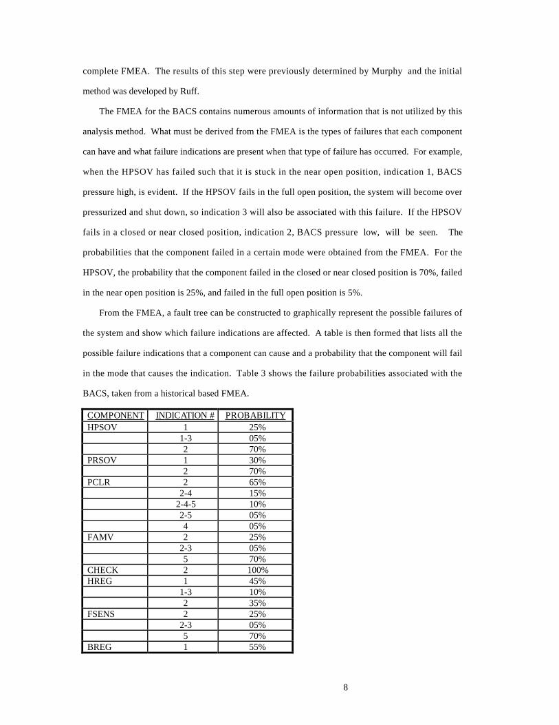
The FMEA for the BACS contains numerous amounts of information that is not utilized by this

analysis method. What must be derived from the FMEA is the types of failures that each component

can have and what failure indications are present when that type of failure has occurred. For example,

when the HPSOV has failed such that it is stuck in the near open position, indication 1, BACS

pressure high, is evident. If the HPSOV fails in the full open position, the system will become over

pressurized and shut down, so indication 3 will also be associated with this failure. If the HPSOV

fails in a closed or near closed position, indication 2, BACS pressure low, will be seen. The

probabilities that the component failed in a certain mode were obtained from the FMEA. For the

HPSOV, the probability that the component failed in the closed or near closed position is 70%, failed

in the near open position is 25%, and failed in the full open position is 5%.

From the FMEA, a fault tree can be constructed to graphically represent the possible failures of

the system and show which failure indications are affected. A table is then formed that lists all the

possible failure indications that a component can cause and a probability that the component will fail

in the mode that causes the indication. Table 3 shows the failure probabilities associated with the

BACS, taken from a historical based FMEA.

C O M P O N E N T I N D I C A T I O N # P R O B A B I L I T Y HPSOV 1 25%

1-3 05%2 70%

PRSOV 1 30%2 70%

PCLR 2 65%2-4 15%

2-4-5 10%2-5 05%4 05%

FAMV 2 25%2-3 05%5 70%

CHECK 2 100%HREG 1 45%

1-3 10%2 35%

FSENS 2 25%2-3 05%5 70%

BREG 1 55%

9

2 35%THERMO 2 10%

3 90%Table 3. 737 BACS Failure Indications

4.2 Predicting Mean Time Between Failures

The objective of this analysis method is to supply estimated MTBF data for the system

components without having historical or test data. Traditionally, component failure rates are

determined either from the underlying physics or from historical data. In the conceptual design phase

of a product, historical or test data is typically not available and the design may not be of enough

detail to perform an analytical failure analysis. To produce a rough estimate of failure rates for

components in a system, we propose extrapolation from the known failure rate data for one

component. By utilizing engineering judgment and common failure patterns, estimated MTBF data

can be generated very early in the design of a product.

The historical MTBF data for the BACS will be compared with the predicted MTBF data that is

developed at the end of this phase.

Step 1

This step yields what is called a failure order, the purpose is to determine which components are

more prone to failure. For the sake of maintaining a general analysis tool, it is assumed that the

specific reasons for component failure can be summarized by the following three Macroscopic reasons

for component failure (Complexity, Use, and Environment). The more complex a component is, the

more likely that it will fail before a less complex component. The more that a component is used, the

more the likelihood of its failure. The harsher the environment that a component is operated in, the

higher the probability that it will fail. Other factors may be more appropriate, as judged by the

engineer, for other systems. A underlying assumption of this method is that all the system

components are equally well designed.

By ranking the components in a system, in the engineering judgment of the engineer, from best to

worst (1 = best, 2 = next best, ..., n = worst) in the areas of complexity, use, and operating

environment, and summing the three numbers together, a failure order for the components within a

10

system is established. The components are ranked from highest numbers to lowest numbers with the

higher numbers indicating higher failure rates. Table 4 shows the analysis performed on the BACS.

C O M P O N E N T C O M P L E X

U S E E N V I R O N

T O T A L

BREG 9 9 7 25HREG 8 2 9 19PRSOV 7 8 6 21HPSOV 6 1 8 15FAMV 5 7 1 13PCLR 2 5 4 11THERMO 3 4 2 9FSENS 4 6 3 13CHECK 1 3 5 9

Table 4. 737 BACS Failure Order Analysis

Table 5 compares the predicted failure order with the actual.

P R E D I C T E D A C T U A L 1. BREG BREG2. PRSOV HREG3. HREG PRSOV4. HPSOV FAMV5. FAMV HPSOV6. FSENS FSENS7. PCLR THERMO8. THERMO PCLR9. CHECK CHECK

Table 5. Predicted vs. Actual Failure Order for the 737 BACS

As can be seen from the chart, this method develops the trend of the components failure rates.

Although this method does not accurately place every component, it does not miss place any

component by more than one place away from where it should be.

The method for predicting the failure order of system components has not been fully developed.

It has not yet been determined if complexity, use, and environment are equally responsible for causing

component failure. The method worked well on the BACS, however, further research in the

development of a failure order is indicated. Increased accuracy in the failure order will greatly increase

the accuracy of the method.

Step 2

11

This step will assign a failure rate to all of the components in the system based on the failure

order and an estimation of a failure rate from one of the components. Even on a newly designed

system, there is usually at least one component that has a known failure rate from its use in a older

system or by extrapolating data from a related component operating in a similar fashion. However, the

reliability of the known failure data is a important to the success of this method and should be

carefully selected.

Within the R&M industry, there is a general rule of thumb called the 80/20 rule. This rule of

thumb states that 80% of your maintenance expenses for a system will be caused by only 20% of the

components. For example, in a system with ten different components it can estimated that 80% of the

maintenance costs will be caused by the two most failed components. Again, this is a rule of thumb

and is by no means accurate nor does it give any clue to the actual maintenance cost. However, the

fact that a general rule like the 80/20 rule exists does give evidence that a predictable pattern of failure

rates exists relative to the components that compose a mechanical systems. The goal of this section is

to utilize historical data to prove the existence of a predictable failure pattern (failure pattern being

defined as the way the failure rates of the different system components relate over the system life-cycle)

for mechanical systems and then utilize that pattern to predict the MTBF's for the BACS components.

For the Boeing 737, six wholly separate mechanical systems were analyzed and failure rate data

plotted from the historical failure data. Two representative plots are shown in Figures 2 and 3, plots

from the other four systems were similar. Each point in the figure represents a component in the

system and the points were evenly spaced between 0 and 1 along the x-axis, most failed at 0 to least

failed at 1. The normalized failure rate, which is the y-axis, for each component was arrived at by

dividing the components actual failure rate by the failure rate of the most failed component in the

system. The line that connects the points in each graph is presented to aid in visualization of the

pattern.

12

0

0.2

0.4

0.6

0.8

1

No

rma

lize

d F

ailu

re R

ate

0 0.2 0.4 0.6 0.8 1 <- Most Failed Least Failed ->

Figure 2. Normalized Failure

Pattern - 737 Flap System

0

0.2

0.4

0.6

0.8

1

Nor

mal

ized

Fai

lure

Rat

e

0 0.2 0.4 0.6 0.8 1 <- Most Failed Least Failed ->

Figure 3. Normalized Failure

Pattern - 737 Fuel Pump System

As can be seen from the two figures, by portraying the historical failure data of the different

mechanical systems in this manner, a similar negative exponential pattern can be seen. From this

generalized failure pattern, a formula can be developed to predict the failure rates of all the components

in a system based on this pattern. An estimated failure rate of one component in the system is

required to provide an actual failure rate prediction instead of a normalized failure rate prediction. The

failure order that was developed in the previous step is needed to properly place the components on the

graph. The formula that was developed for failure rate prediction is based on exponential functions to

produce a curve that simulates the negative exponential pattern shown in the above graphs, it was

created by displaying all the available failure data on one graph and developing a formula to best fit

the average of that data.

FR

FRe e

e e

e e

e e

i

known

x

x

i

known

=

−−

�

���

�

���

−−

�

���

�

���

− −

−

− −

−

0375

0375

1

0 1

1

0 1

.

.(1)

where xi is the x-axis position of the component in question, and xknown is the x-axis position of

component for which the Failure Rate is known. The 0.375 factor is a result of curve fitting. The x-

13

axis position of all the components in the system are generated by evenly spacing the components

between 0 and one, most failed at zero to least failed at one, following the failure order that was

previously determined. The known component failure rate should be as far to the left on the curve as

possible for accuracy reasons.

Figure 4 shows the prediction curve from the formula developed above and the actual and

predicted failure rates for the BACS. The failure rate for the BREG was used as the known failure

rate.

0

0.05

0.1

0.15

0.2

Fai

lure

Rat

e/10

00 h

rs

0

0.05

0.1

0.15

0.2

0 0.2 0.4 0.6 0.8 1 <-- Most Failed Least Failed -->

Prediction Curve Actual Predicted

BREG

PRSOV

HREG

HPSOV FAMV

FSENS

PCLR

THERMO

CHECK

Figure 4. MTBF Prediction

By inverting the predicted failure rates from the Figure 4, a predicted MTBF for each component

is arrived at. Table 6 lists the predicted MTBF's versus the actual MTBF's for the BACS

components.

C O M P O N E N T P R E D I C T E D M T B F

A C T U A L M T B F

BREG 5980 5980PRSOV 14500 20220HREG 20600 11840HPSOV 28900 22348FAMV 39900 21489FSENS 59600 28232PCLR 91200 235348THERMO 214000 45762CHECK 2720000 471934

Table 6. Predicted vs. Actual MTBF's for the 737 BACS

There is expected error associated with this prediction method. The actual data was generated

from three years of maintenance logs across the entire 737 fleet, while the predicted data can be

generated in the conceptual design phase of product development. The accuracy of the predicted

14

MTBF data can be improved by improving the failure order that was previously developed. Current

research, as discussed in the summary, is attempting to refine this prediction technique.

4.3 Predicting Mean Time Between Maintenance Actions

For each unique failure indication, there is a diagnostic process that must be performed by the

maintenance personnel. The developed method attempts to simulate that diagnostic process and yields

a maintenance rate for all the possible components for that failure indication. The method that is

presented must be performed for each different failure indication to find the overall maintenance rates,

and conversely the MTBMA's, for each component.

The method used to predict MTBMA is a modified version of that developed by Wong (1994).

The main modifications to this method is the inclusion of the probabilities that a component failed in

a particular mode to cause a particular failure indication ( PF indi | ). This data was developed in the

system modeling phase and is listed in table 3. Also, the end result of the method utilized here is a

prediction of MTBMA data, while Wong attempted to solve directly for cost.

The average time to perform a maintenance action (ATFMA) for each component is needed to

perform this phase of the analysis. The ATFMA data is assumed to be known or arrived at by some

other method. For the BACS, the ATFMA's were developed from historical data by The Boeing

Company and are listed below.

C O M P O N E N T A T F M A ( h r s . ) HPSOV 0.40PRSOV 0.89PCLR 43.00FAMV 1.33CHECK 1.00HREG 2.00FSENS 0.05BREG 3.00THERMO 0.05

Table 7. ATFMA of the 737 BACS components

Other data that is needed is the predicted failure rate data from the previous phase.

The method presented here contains four steps. The first step finds the probability that a

particular failure indication will occur. The next step develops an optimum checking order to diagnose

system components and the checking order is utilized along with failure data to determine the

probabilities that a particular component will be the cause of a failure indication. The final step is to

15

determine the Maintenance Rate for each component per indication, which is a function of the

probability of the indication occurring multiplied by the probabilities that the previous checked

components in the diagnostic process have not failed.

Step 1

The probability of each failure indication occurring must be computed. The probability of a

failure indication occurring is a function of the failure rates of all the components that can cause that

given failure indication and the associated probabilities that the components will fail in a mode that

will cause the given failure indication. The formula below is used to find the probability of an

indication ( Pind ).

( )( )( )P FR PF indind i ii

n

= − −=

⊆1 11

| (2)

Where FRi is the failure rate of the component, which is arrived at by inverting the predicted

MTBF that was developed in the previous phase, and PF indi | is the probability that the component

failed in the mode to produce this given failure indication.

For example, four components (BREG, PRSOV, HREG, HPSOV) can fail in a mode that

causes indication 1, BACS pressure high. The probability of indication 1 occurring in 1000 flight

hours is presented.

( )( )( )P FR PF indind i ii

11

4

1 1 1= − −=

⊆ |

Where i=1 is BREG, i=2 is PRSOV, i=3 is HREG, and i=4 is HPSOV

( )( )( ) ( )( )( )( )( )( ) ( )( )( )

Pind1 11 01673 0 55 1 0 0688 0 30

1 0 0487 0 1 0 0346 0 25= −

− −

− −

���

�

↵√√

. . . .

. .45 . .

Pind1 013773= .

Step 2

The checking order index must be established to simulate the trouble shooting process. The

variables of failure rate and maintenance time were selected because they are the biggest factors that

influence a mechanics choice to check one component before another. This step will determine the

16

order in which components should be checked based on probabilities of failure and maintenance times.

The formula for the checking order index is presented.

( )( )CO

FR PF ind

ATFMAiindi i

|

|= (3)

Where ATFMA is the Average Time For Maintenance Action. A checking order index must be

determined for each candidate component for a given failure indication. The components are then

assumed to be checked in order from highest checking order index to lowest checking order index so

the analysis method can have a repeatable result. Some situations may determine that failure rate or

maintenance times are more important than the other variable. In this situation, the engineer should

weight the important variable to his/her informed discretion. No weighting was used for the analysis

on the BACS.

( )( ) ( )( )CO

FR PF ind

ATFMABREGBREG BREG

BREG

= = =| . .

..

1 01673 0 55

3000 0306

( )( ) ( )( )CO

FR PF ind

ATFMAPRSOVPRSOV PRSOV

PRSOV

= = =| . .

..

1 0 0688 0 30

0890 0232

( )( ) ( )( )CO

FR PF ind

ATFMAHREGHREG HREG

HREG

= = =| . .45

..

1 0 0487 0

2 000 0109

( )( ) ( )( )CO

FR PF ind

ATFMAHPSOVHPSOV HPSOV

HPSOV

= = =| . .

.40.

1 0 0346 0 25

00 0216

So the order in which the components should be checked for indication 1 is, BREG: PRSOV:

HPSOV: HREG.

Step 3

The probability that a given component is the cause of the failure indication must now be

determined by the formula listed below.

( )( )( )( )P

FR PF ind

FR PF indcompindcomp comp

i iunchecked

|

|

|=

� (4)

Aside from the inclusion of the probability of a component failing in a particular mode, this

formula was further modified from that of Wong (1994) to consider unchecked components only.

When a component is checked, it is determined if that component is the cause of the failure or not. If

17

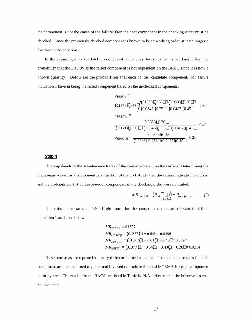
the component is not the cause of the failure, then the next component in the checking order must be

checked. Since the previously checked component is known to be in working order, it is no longer a

function in the equation.

In the example, once the BREG is checked and if it is found to be in working order, the

probability that the PRSOV is the failed component is not dependent on the BREG since it is now a

known quantity. Below are the probabilities that each of the candidate components for failure

indication 1 have in being the failed component based on the unchecked components.

( )( )( )( ) ( )( )( )( ) ( )( )

( )( )( )( ) ( )( ) ( )( )

( )( )( )( ) ( )( )

P

P

P

BREG

PRSOV

HPSOV

|

|

|

. .. . . .

. . . .45.

. .

. . . . . .45.40

. .

. . . .45.

1

1

1

01673 0 5501673 0 55 0 0688 0 30

0 0346 0 25 0 0487 00 64

0 0688 0 30

0 0688 0 30 0 0346 0 25 0 0487 00

0 0346 0 25

0 0346 0 25 0 0487 00 28

=+ +

+=

=

+ +=

=+

=

Step 4

This step develops the Maintenance Rates of the components within the system. Determining the

maintenance rate for a component is a function of the probability that the failure indication occurred

and the probabilities that all the previous components in the checking order were not failed.

( ) ( )MR P Pcompind ind compindchecked

| |= −⊆ 1 (5)

The maintenance rates per 1000 flight hours for the components that are relevant to failure

indication 1 are listed below.

( )( )( )( )( )

( )( )( )( )

MR

MR

MR

MR

BREG

PRSOV

HPSOV

HREG

|

|

|

|

.

. . .

. . .40 .

. . .40 . .

1

1

1

1

01377

01377 1 0 64 0 0496

01377 1 0 64 1 0 0 0297

01377 1 0 64 1 0 1 0 28 0 0214

=

= − == − − =

= − − − =

These four steps are repeated for every different failure indication. The maintenance rates for each

component are then summed together and inverted to produce the total MTBMA for each component

in the system. The results for the BACS are listed in Table 8. N/A indicates that the information was

not available.

18

C O M P O N E N T P R E D I C T E D M T B M A

A C T U A L M T B M A

BREG 4507 N/APRSOV 5585 10515HREG 18082 4000HPSOV 5300 3154FAMV 31496 9000FSENS 5337 31544PCLR 94905 27800THERMO 29720 N/ACHECK 2724796 N/A

Table 8. Actual vs. Predicted MTBMA for the 737 BACS

The results that were developed by this method seem fairly erred when compared to the actual

data. MTBMA data is not nearly as important to maintenance cost issues as MTBF or MTBUR data,

however, MTBMA data is necessary to fully use the Line Labor Cost Formula that is utilized by this

method. In the absence of another, more accurate, method to determine MTBMA, the presented

method was utilized so a fully predicted cost analysis could be performed.

4.4 Predicting Mean Time Between Unscheduled Removal

This analysis method was developed by Murphy (1997). The only deviation from Murphy's

method is the utilization of Predicted MTBF's instead of Historical MTBF's for the components in the

system.

Step 1

Murphy (1997) separates unscheduled component removals into two categories, justified and

unjustified. The justified unscheduled removals are equivalent to the failure rates of each component,

so the is equal to the MTBF for each component.

MTBUR comp MTBF compj | |= (6)

Step 2

The unjustified unscheduled removal of a component is due to misdiagnosis of the system, it

represents the removal of a component that was thought to be failed but in actuality was not. Murphy

presents a formula that specifies unjustified MTBUR as a function of the MTBF's of the other

candidate components for a failure indication and the probability of detection.

19

MTBUR ind

MTBF

PDujcomps

other

icomp

| =�

(7)

Where,

( )( )( )

( )( )( )

PD

FR PF ind

LLHPR SLHPR

FR PF ind

LLHPR SLHPR

i

i i

i i

i

n= +

+=�

|

|

1

(8)

Step 3

When both justified and unjustified MTBUR’s are known, the actual MTBUR can be

calculated as shown below.

MTBUR

MTBUR MTBUR

actual

j uj

=+

11 1 (9)

The MTBUR results for the BACS are listed in Table 9.

COMPONENT PREDICTEDMTBUR

ACTUALMTBUR

BREG 4488 4654PRSOV 8119 15664HREG 8900 8455HPSOV 15817 9996FAMV 29557 13520FSENS 26998 21256PCLR 81935 90987THERMO 172391 19957CHECK 1004908 471934

Table 9. Predicted vs. Actual MTBUR for the 737 BACS

The MTBUR results that were developed from the predicted MTBF data are equivalent to the

MTBUR data that was developed by Murphy using historical MTBF data. The MTBUR data is the

main influence in figuring maintenance costs so it is a promising occurrence to get similar results from

predicted MTBF data as is received from actual MTBF data.

20

4.5 Labor Cost Evaluation

Once the MTBF's, MTBUR's, and MTBMA's are known for each component in a system, a cost

analysis can be performed. The formulas for Line Maintenance Cost and Shop Maintenance Cost

where developed by the Boeing Company, however, Boeing utilized the formulas to figure the cost for

an airplane fleet per year. The formulas utilized here were simplified to solve for cost per 1000 flight

hours of a single plane.

Step 1

The formula for computing line labor maintenance cost is as follows.

Line Labor Cost = (hourly line labor cost)LLHPR

MTBUR

ATFMA

MTBMA��

�↵√

+ ��

�↵√

��

�↵√

(10)

Step 2

The formula for computing shop labor maintenance cost is as follows.

Shop Labor Cost = (hourly shop labor cost)SLHPR

MTBUR��

�↵√ (11)

Step 3

The total labor cost is found by summing the Shop Labor Cost and Line Labor Cost together

for all the components in the system. Historically, the BACS requires a labor cost of $517.00 per

1000 flight hours and the final cost developed from the prediction method presented is $416.00 per

1000 flight hours, an error of 20%. Although the error of the result is fairly large, the

resulting cost analysis is still of value. It must be remembered that the final labor cost was fully

predicted by the analysis method. Detailed historical data or laboratory test data is not required. As

will be demonstrated in the succeeding section, the analysis method is sensitive to prospective changes

in the system as well. This ability makes the method useful as a design tool to compare the up front

cost of a design change or a competing design idea versus the life time savings that the change will

produce.

21

5 ANALYSIS OF PROPOSED CHANGES TO BLEED AIR CONTROL SYSTEM

For an analysis method to be useful as a design tool, it must be coarse enough to yield reasonable

results without precise data, yet sensitive enough to pick-up small changes and produce the effect that

the change will induce. This section demonstrates the ability of the method to predict the effect of

design changes on maintainability costs. Four prospective changes to the BACS are examined in this

section. Each design change is considered independently of the other design changes

5.1 Design Change #1, PRSOV Failed Closed Indication

This design change adds a mechanical switch to the PRSOV that is depressed when the valve is in

the closed or near closed position. This switch gives another failure indication to the pilots if the

PRSOV is stuck in the closed position. This change was modeled by adding a failure indication 6 to

represent the PRSOV stuck in the closed position. This design change effectively removes the

PRSOV from the trouble-shooting process for failure indication 2 since the switch (indication 6) will

inform the mechanic if the PRSOV has failed in this mode or not.

By removing the PRSOV from indication 2, the probability of that indication occurring dropped

from .1562 to .1135 per 1000 flight hours and the failure probabilities of the components prior to the

PRSOV in the checking were increased slightly. This had the effect of raising the MTBMA's for all

the components in the BACS and greatly increasing the MTBMA for the PRSOV from 5585 hours to

10230 hours. A similar change in MTBUR is produced by the addition of the PRSOV switch. There

is a slight increase in MTBUR for all components and the MTBUR for the PRSOV changes from

8199 hours to 11486 hours. The result was a predicted 6% labor cost savings.

5.2 Design Change #2, Monitor Pressure Data to Determine PRSOV Failure

This design changes involves the addition of a computer method to monitor the bleed air pressure

gauge to determine PRSOV failure or not. This change was modeled as supplying failure indication

7, PRSOV failed.

The changes to the system analysis were very similar to Design Change #1. The MTBUR's and

MTBMA's were reduced further and the MTBUR and MTBMA for the PRSOV were both changed to

14532 hours, the same as the MTBF. Since there is now an indication that directly determines

22

PRSOV failure, there is no need to even check the component unless it is known to be failed. A 10%

labor cost savings was produced by this design change.

5.3 Design Change #3, External Marker on PRSOV to Indicate Valve Position

This design change placed an indicator on the outside of the PRSOV that showed valve position.

Although this change does not give another failure indication to the system, it does aid in the

diagnosis of the system. This change would allow diagnosis of the PRSOV on physical inspection

alone and prevent the need to remove the valve for inspection. This was modeled by reducing the

ATFMA for the PRSOV to 0.05 hours.

The effect that this change had on the calculations was changing the checking order for the failure

indications that involved the PRSOV. The effect that this had was lowering the MTBMA of the

PRSOV from 5585 hours to 3402 hours, since it is now first in the checking orders that it is involved

in. The MTBMA for the other components increased or decreased slightly. This is because the

change in the checking order changed the probabilities of the checked components being the failed

components. The predicted labor cost savings from this design change was 1.8%.

5.4 Design Change #4, Monitor Current to BREG to Determine Failure

This design change calls for the introduction of a computer logic card to monitor the current being

supplied to the BREG. By monitoring the current, it can be determined if the BREG has failed or

not. This was modeled in the formula by adding indication 8, BREG failure, to the possible failure

indications.

As with the PRSOV in design change #2, this design change effectively removes the BREG from

being a candidate in indication 1 and indication 2. Since the BREG has the highest failure rate in

the system, the isolation of this component drastically lowers the probability of indication 1 and 2

occurring, They change from 0.1377 and 0.1562 to 0.0504 and .1038 respectively. Also, the

probabilities of the checked component being the failed component noticeably increase with the BREG

removed from the equation. The MTBUR's of all the components are raised as well due to the reduces

ambiguity of the system. These effects combine to produce a 18.5% labor cost savings with this

design change.

23

6 CONCLUSIONS AND RECOMMENDATIONS

The end result of this research is a tool to aid in the design of a product based on life-cycle cost.

The developed method calculates the life-cycle labor cost that is to be expected while maintaining the

product. The developed method is also capable of comparing competing designs or design changes

based on cost. Although the inclusion of the capital costs of the product was not part of this research,

it is relatively easy to quantify and should be used to fully analyze life-cycle cost savings. This

method provides the designer the ability to make more informed decisions earlier in the design

process, so design changes can be made in the most inexpensive manner possible.

The assumption of knowing the SLHPR, LLHPR, ATFMA, and having a detailed FMEA in the

early stages of the design is fairly major. However, the Service Mode Analysis (Eubanks, 1993) that

is being developed addresses these variables and issues in a predictive manner. With the inclusion of a

method that predicts the variables that were assumed known in this research, the predictive ability of

this research increases greatly.

Further research in this area should concentrate in many different areas. The method that was

developed here is fairly long and tedious when performed by hand. Developing this method into a

computer program would increase its ease of use and greatly decrease the analysis time required. The

inclusion of a Service Modes Analysis would also be of benefit in the future. The inclusion of Service

Modes Analysis would effectively predict everything impacting the life-cycle cost of a product with

the bare minimum of assumptions. Lastly, more research should be placed into the assigning of the

failure ranking (Section 4.2). Increased accuracy in this area would greatly increase the accuracy of the

entire method.

ACKNOWLEDGMENTS

This material is based on work supported by the National Science Foundation under grant number

DMII-9309193. In addition, the authors would like to thank the Boeing Company for their assistance

on this project.

REFERENCES

24

Blanchard, Benjamin S., Verma, Dinesh, Peterson, Elmer L., 1995, Maintainability: A Key To

Effective Serviceability and Maintenance Management, John Wiley and Sons, New York.

Bryan, Christopher, Eubanks, Charles, Ishii, Kosuke, 1992, "Design For Serviceability Expert

System", ", Proc. of the 13th International Computers in Engineering Conference, pp91-98.

Clark, G. E. , Paasch, R. K., 1996, "Diagnostic Modeling and Diagnosability Evaluation of

Mechanical Systems", Journal of Mechanical Design, 118 (3): pp. 425-431.

Di Marko, Patrick, Eubanks, Charles F., Ishii, Kos, 1995, "Service Modes and Effects Analysis:

Integration of Failure Analysis and Serviceability Design", Proc. of the 15th International Computers

in Engineering Conference, Boston, MA, pp. 833-840.

Eubanks, Charles F., Ishii, Kosuke, 1993, "AI Methods for Life-Cycle Serviceability Design of

Mechanical Systems", Artificial Intelligence in Engineering, 8(2): pp127-140.

Gershenson, John, Ishii, Kosuke, 1991, "Life-Cycle Serviceability Design", Proc. of the 3rd

International Conference on Design Theory and Methodology, pp127-34.

Goldberg, Saul, Horton, William F., Rose, Virgil G., 1987, "Analysis of Feeder Service

Reliability using Component Failure Rates", IEEE Transactions on Power Delivery, 2, pp1292-6.

Leemis, Lawrence A., 1995, Reliability: Probabilistic Models and Statistical Methods, Prentice-

Hall, New Jersey.

Marks, Matthew D., Eubanks, Charles F., Ishii, Kos, 1993, "Life-Cycle Clumping of Product

Designs for Ownership and Retirement", Proc. of the 5th International Conference on Design Theory

and Methodology, Albuquerque, NM, pp83-90.

Murphy, M. D., Paasch, R. K., 1997, "Reliability Centered Prediction Technique for Diagnostic

Modeling and Improvement", Research in Engineering Design (1997) 9: 35-45.

Ruff, D. N., Paasch, R. K., 1997, "Evaluation of Failure Diagnosis in Conceptual Design of

Mechanical Systems", Journal of Mechanical Design, Vol. 119, No. 1, pp. 57-64

Wong, Bryan, 1994, "Diagnosability Analysis for Wong, Wong, Bryan, 1994, ”Mechanical

Systems and Human Factors in Diagnosability", M.S. Thesis, Department of Mechanical Engineering,

Oregon State University, Corvallis, Oregon