EU-10

0018-9464 © 2015 IEEE. Personal use is permitted, but republication/redistribution requires IEEE permission.

See http://www.ieee.org/publications_standards/publications/rights/index.html for more information. (Inserted by IEEE.)

1

Analytical Functions of Magnetization Curves

for High Magnetic Permeability Materials

Mehran Mirzaei1, and Pavel Ripka1

1 Faculty of Electrical Engineering, Czech Technical University, 16627 Prague, Czech Republic

In this paper, combined rational and power functions are used to represent magnetization curves of high magnetic permeability ferromagnetic materials. The proposed functions cover much wider range of magnetic fie lds than functions currently used in

simulation software packages. The objective is to present simple functions for approximation of magnetization curves with minimum

number of unknown constants. The calculated functions are finally compared with measured magnetization curves to validate the

precision in a wide fie ld range from 10 -2 to 106 A/m.

Index Terms— Analytical functions, high magnetic permeability materials, curve fitting, magnetization curves .

I. INTRODUCTION

HE most industrial used ferromagnetic materials could be

categorized to two major groups of metallic and non-

metallic magnetic materials. Non-metallic magnetic materials

are composed of Ferrite families. Metallic magnetic materials

are mostly iron alloys families such as cast iron and steels, low

carbon steels, silicon steels, nickel based iron alloy and cobalt

based iron alloy [1].

The nickel based iron alloys (Ni-Fe) have special industrial

applications because of very high maximum permeability with

small hysteresis losses and considerably high electrical

resistivity. The high magnetic permeability is caused by small

hysteresis loop and very low magnetic coercive force, which

makes sharp changing of magnetic flux density at low

magnetic field strength. These characteristics shows suitable

applications of Ni-Fe alloy for telecommunications functions.

They have also numerous industrial applications such as

magnetic sensors, high efficiency transformers, magnetic

recording heads and magnetic shields [1] -[3].

Analytical representations of the magnetization and B-H

curve of magnetic materials are used for magnetic modeling,

numerical analysis and design process. Using approximated

mathematical B-H curve could help for first design step of

magnetic devices [3]. It gives apparent and fast picture of

maximum magnetic relative permeability and magnetic

saturation without B-H data table. B-H curve could be

represented by different closed-form formula [4]. Several

publications have presented detailed analysis for B-H curve

modeling, for example, rational function [4] - [7] and

exponential function [8] - [10]. The modeled magnetic

materials for B-H functions were silicon steel laminations and

solid irons and steels in [4] - [10], which have small magnetic

permeability especially at low magnetic fields. Papers [5] and

[7] are mostly devoted to optimization of curve fitting.

Piecewise modeling of B-H curve with high precision is also

presented [11] but it does not obtain one closed-form equation.

Power functions could precisely model a fraction part of B-H

curve but not the whole B-H curve from low field part to

highly saturated part [12]-[14].

In this paper rational function and power function are

combined for modeling of very high permeability B-H curves.

The constants of the proposed function are calculated by curve

fitting tool. It is shown that the proposed function can

accurately fit the measured B-H curve despite its not-

complicated equation. Finally, the proposed function is used

for curve fitting of modified B-H curve corresponding to

fundamental component of flux density for AC analysis.

II. BASIC STUDY

A. Assumptions

Magnetization parameter, J versus magnetic field strength

and relative magnetic permeabilities are represented as

following:

dH

dH

dH

Hd

dH

dB

H

B

HBJ

ar

ar

ar

dr

ar

,

,

,0

00

,

0

,

0

).(11

1

.

(1)

where, 0 , ar , and dr , are free space magnetic

permeability, apparent relative permeability and differential

relative permeability. In order to calculate analytical function,

it must be considered that magnetization, J is becoming

constant when magnetic field strength, H is moving toward

infinite and apparent and differential relative permeabilities

must have one maxima between magnetic field strength, H=0

until H = ∞. The former condition is necessary to model

Rayleigh region of the B-H curve.

B. Basic function

First order rational function is simple analytical function,

which could match with B-H curve from low field to highly

saturation. The main disadvantage of first order rational

function is that it is not able to model Rayleigh region and

relative permeability maxima could not be reproduced. In

order to improve it, power of parameter, x must be adjusted to

value above 1:

T

Corresponding author: M. Mirzaei (e-mail: mirzameh@fel.cvut.cz).

EU-10

2

),)((,1

)( HxJxfxa

xaxf

b

b

(2)

where, a , a' and b are constants. The relative magnetic

permeability for basic function (2) is as following:

21

0

1

2

0

,,

1

0

,

1

11

1

)1(1

1

11

)),((,1

)(

b

b

b

b

b

ardr

b

b

ar

b

b

xa

xba

xaxa

xab

xa

xa

HxxfJxa

xaxf

(3)

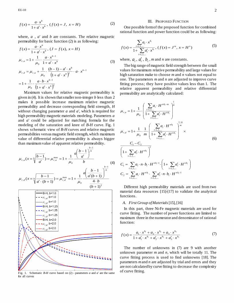
Maximum values for relative magnetic permeability is

given in (4). It is shown that smaller non-integer b less than 2

makes it possible increase maximum relative magnetic

permeability and decrease corresponding field strength, H

without changing parameter a and a', which is required for

high permeability magnetic materials modeling. Parameters a

and a' could be adjusted for matching formula for the

modeling of the saturation and knee of B-H curve. Fig. 1

shows schematic view of B-H curves and relative magnetic

permeabilities versus magnetic field strength, which maximum

value of differential relative permeability is always bigger

than maximum value of apparent relative permeability.

2

1

0

max

,,

1

0

max

,,

)1(

4

)1(

1

11)

)1(

1(

1

11)

1(

b

b

ba

ba

ba

bx

b

a

ba

a

bx

b

b

drb

dr

b

b

arb

ar

(4)

Fig. 1. Schematic B-H curve based on (2) - parameters a and a' are the same for all curves

III. PROPOSED FUNCTION

One possible form of the proposed function for combined

rational function and power function could be as following:

),)((,1

)(

,...2,1

,...2,1 nm

i

b

i

i

b

i

HxJxfxa

xa

xfi

i

(5)

where, ia ,

ia , ib , m and n are constants.

The big range of magnetic field strength between the small

values for maximum relative permeability and large values for

high saturation make to choose m and n values not equal to

one. The parameters m and n are adjusted to improve curve

fitting process; they have positive values less than 1. The

relative apparent permeability and relative differential

permeability are analytically calculated:

,...2,1

1

,...2,1

2

,...2,1,...2,1

1

1

2

,...2,1

21

1

,...2,1

,...2,1

0

,

1

,...2,1

,...2,1

0

,

1

1

1

111

1

11

i

bn

ii

i

bn

i

i

bn

i

i

bn

ii

i

bn

i

m

m

i

bn

i

i

bn

i

dr

m

i

bn

i

i

mbn

i

ar

ii

ii

i

i

i

i

i

HbnaHaC

HaHbnaC

Ha

CC

Ha

Ha

m

Ha

Ha

(6)

Different high permeability materials are used from two

material data resources [15]-[17] to validate the analytical

functions.

A. First Group of Materials [15], [16]

In this part, three Ni-Fe magnetic materials are used for

curve fitting. The number of power functions are limited to

maximum three in the numerator and denominator of rational

function:

321

321

321

321

1)(

bbb

bbb

xaxaxa

xaxaxaxf

(7)

The number of unknowns in (7) are 9 with another

unknown parameter m and n, which will be totally 11. The

curve fitting process is used to find unknowns [18]. The

parameters m and n are adjusted by trial and errors and they

are not calculated by curve fitting to decrease the complexity

of curve fitting.

EU-10

3

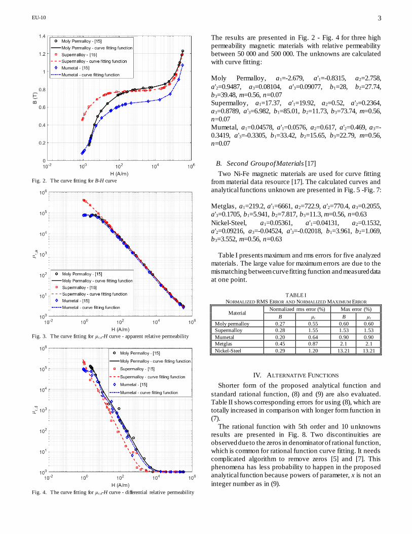
Fig. 2. The curve fitting for B-H curve

Fig. 3. The curve fitting for µr,a-H curve - apparent relative permeability

Fig. 4. The curve fitting for µr,d-H curve - differential relative permeability

The results are presented in Fig. 2 - Fig. 4 for three high

permeability magnetic materials with relative permeability

between 50 000 and 500 000. The unknowns are calculated

with curve fitting:

Moly Permalloy, a1=-2.679, a'1=-0.8315, a2=2.758,

a'2=0.9487, a3=0.08104, a'3=0.09077, b1=28, b2=27.74,

b3=39.48, m=0.56, n=0.07

Supermalloy, a1=17.37, a'1=19.92, a2=0.52, a'2=0.2364,

a3=0.8789, a'3=6.982, b1=85.01, b2=11.73, b3=73.74, m=0.56,

n=0.07

Mumetal, a1=0.04578, a'1=0.0576, a2=0.617, a'2=0.469, a3=-

0.3419, a'3=-0.3305, b1=33.42, b2=15.65, b3=22.79, m=0.56,

n=0.07

B. Second Group of Materials [17]

Two Ni-Fe magnetic materials are used for curve fitting

from material data resource [17]. The calculated curves and

analytical functions unknown are presented in Fig. 5 -Fig. 7:

Metglas, a1=219.2, a'1=6661, a2=722.9, a'2=770.4, a3=0.2055,

a'3=0.1705, b1=5.941, b2=7.817, b3=11.3, m=0.56, n=0.63

Nickel-Steel, a1=0.05361, a'1=0.04131, a2=0.1532,

a'2=0.09216, a3=-0.04524, a'3=-0.02018, b1=3.961, b2=1.069,

b3=3.552, m=0.56, n=0.63

Table I presents maximum and rms errors for five analyzed

materials. The large value for maximum errors are due to the

mismatching between curve fitting function and measured data

at one point.

TABLE I

NORMALIZED RMS ERROR AND NORMALIZED MAXIMUM ERROR

Material Normalized rms error (%) Max error (%)

B µr B µr

Moly permalloy 0.27 0.55 0.60 0.60

Supermalloy 0.28 1.55 1.53 1.53

Mumetal 0.20 0.64 0.90 0.90

Metglas 0.45 0.87 2.1 2.1

Nickel-Steel 0.29 1.20 13.21 13.21

IV. ALTERNATIVE FUNCTIONS

Shorter form of the proposed analytical function and

standard rational function, (8) and (9) are also evaluated.

Table II shows corresponding errors for using (8), which are

totally increased in comparison with longer form function in

(7).

The rational function with 5th order and 10 unknowns

results are presented in Fig. 8. Two discontinuities are

observed due to the zeros in denominator of rational function,

which is common for rational function curve fitting. It needs

complicated algorithm to remove zeros [5] and [7]. This

phenomena has less probability to happen in the proposed

analytical function because powers of parameter, x is not an

integer number as in (9).

EU-10

4

Fig. 5. The curve fitting for B-H curve

Fig. 6. The curve fitting for µr,a-H curve - apparent relative permeability

Fig. 7. The curve fitting for µr,d-H curve - differential relative permeability

Fig. 8. The curve fitting for B-H curve - calculated rational function, (9) unknowns: a1=0.7828, a2=-228.1, a3=969.1, a4=-2581, a5=3194, a'1 =-290.6,

a'2 =937.9, a'3 =-1792, a'4 = 634, a'5 = 3323

),)((,1

)(21

21

21

21 nm

bb

bb

HxJxfxaxa

xaxaxf

(8)

),)((

1)(

5

5

4

4

3

3

2

21

5

5

4

4

3

3

2

21

HxJxf

xaxaxaxaxa

xaxaxaxaxaxf

(9)

TABLE II

NORMALIZED RMS ERROR AND NORMALIZED MAXIMUM ERROR - FUNCTION

WITH LESS UNKNOWNS

Material Normalized rms error (%) Max error (%)

B µr B µr

Moly permalloy 0.59 2.06 2.62 2.62

Supermalloy 0.26 0.684 1.32 1.32

Mumetal 1.26 3.15 6.63 6.63

Metglas 3.32 6.56 8.6 8.6

Nickel-Steel 1.0 15.35 98.9 98.9

The unknowns are calculated for (8) with curve fitting:

Moly Permalloy, a1=4.256, a'1=4.894, a2=-4.337, a'2=-5.592,

b1=2.527, b2=1.222, m=0.56, n=0.07

Supermalloy, a1=0.6312, a'1=0.7258, a2=-0.4198, a'2=-1.408,

b1=4.737, b2=0.1899, m=0.56, n=0.07

Mumetal, a1=0.4232, a'1=0.5815, a2=0.003329, a'2=0.004199,

b1=15.23, b2=30.72, m=0.56, n=0.07

Metglas, a1= 0.000468, a'1= 0.0004867, a2= -0.0002592, a'2= -

0.9988, b1= 0.6358, b2= 0.000674, m=0.56, n=0.63

Nickel-Steel, a1=0.1039, a'1=0.09879, a2=0.001024, a'2=

0.0008324, b1= 2.629, b2= 4.219, m=0.56, n=0.63

Other functions comparison such as exponential functions

or closed-form trigonometric functions are skipped to be

presented in this paper, which could give less precision rather

than rational function.

EU-10

5

V. MODIFIED B-H CURVE

A modified B-H curve is used when magnetic materials are

involved in AC or time harmonic analysis especially with high

nonlinearity. The B-H curve is modified to B1-H, which B1 is

fundamental component of flux density when field strength

changes in sinusoidal form [14] and [15].

Fig. 9 and Fig. 10 show B1-H curve from measured values

and curve fitting function. The results are promising for B1-H

curve. The calculated results for maximum error of flux

density and relative permeability, rms error of flux density and

relative permeability are, 1.41% and 1.41%, 0.29% and

0.70%, respectively.

Fig. 9. The curve fitting for B1-H curve

Fig. 10. The curve fitting for µr,a,1-H curve - apparent relative permeability

VI. CONCLUSION

New analytical function has been presented, which could

precisely model B-H curve and relative permeability. The

selected materials were high magnetic permeability Ni-Fe

alloys but the presented analytical function could also be used

for other magnetic materials. The main advantages of

presented function are its compact format and high precision

even with low number of unknowns for curve fitting. The

typical value of rms error ranges from 0.3 to 1.6 %.

Standard rational function was compared with the proposed

analytical function, which has disadvantage of probable zeros

in denominator and discontinuities in the modeled curve.

Exponential functions for B-H curve modeling are not as

precise as rational functions. The unknowns of the proposed

analytical function could be calculated with simple curve

fitting function.

Compatibility of the proposed analytical function has been

presented for modified B-H curve corresponding to

fundamental component of flux density, which shows also

high precision.

REFERENCES

[1] C.W. Chen, Magnetism And Metallurgy Of Soft Magnetic Materials, North Holland , 1st January 1977

[2] P. Ripka, Magnetic Sensors and Magnetometers, Artech House, Jan 1, 2001 - Technology & Engineering - 494 pages

[3] S. Tumanski, Handbook of Magnetic Measurements, June 23, 2011 by CRC Press Reference - 404 Pages

[4] F. C. Trutt, E. A. Erdélyi, and R. E. Hopkins, “ Representation of the

magnetization characteristic of dc machines for computer use,” IEEE Trans. Power App. Syst., vol. 87, no. 3, pp. 665–669, Mar. 1968.

[5] G. F. T. Widger, “ Representation of magnetisation curves over extensive range by rational-fraction approximations,” Proc. Inst. Elect. Eng., vol.

116, no. 1, pp. 156–160, Jan. 1969. [6] J. Rivas, J. M. Zamarro, E. Martín, and C. Pereira, “ Simple

approximation for magnetization curves and hysteresis loops,” IEEE Trans. Magn., vol. 17, no. 4, pp. 1498–1502, Jul. 1981.

[7] Patrick Diez andJ. P. Webb,"A Rational Approach to B – H Curve Representation", IEEE Trans. on Magn. , Year: 2016, Volume: 52,

Issue: 3 [8] M. K. El-Sherbiny, "Representation of the magnetization characteristic

by a sum of exponentials", IEEE Trans. Magn., vol. MAG-9, no. 1, pp. 60-61, Mar. 1973.

[9] W. K. Macfadyen, R. R. S. Simpson, R. D. Slater, W. S. Wood, "Representation of magnetization curves by exponential series", Proc.

IEE, vol. 120, no. 8, pp. 902-904, 1973. [10] J. R. Brauer, “ Simple equations for the magnetization and reluctivity

curves of steel,” IEEE Trans. Magn., vol. 11, no. 1, p. 81, Jan. 1975. [11] P. Diez, "Symmetric Invertible B – H Curves Using Piecewise Linear

Rationals", IEEE Trans. on Magn. , Year: 2017, Volume: 53, Issue: 6 [12] Nejman, L.R., Skin effect in ferromagnetic bodies, GEI, Moscow-

Leningrad, 1949 [13] J Lammeraner, and M Stafl, Eddy Currents, Published by Iliffe, 1967

[14] S. A. Nasar; G. Y. Xiong; Z. X. Fu, "Eddy-current losses in a tubular linear induction motor", IEEE Trans. on Magn., 1994, Volume:

30, Issue: 4, Pages: 1437 - 1445, [15] http://www.femm.info/wiki/Documentation/

[16] Metals Handbook, Volume 1, American Society for Metals, 1966 [17] Free BH Curves, accessed on March 02, 2018. [Online]. Available:

http://www.magweb.us/free-bh-curves/ [18] https://www.mathworks.com/products/curvefitting.html