Analytical Formulae for Radar Cross Section of Flat Plates in Near Field and Normal Incidence

Progress In Electromagnetics Research B, Vol. 9, 263–279, 2008

ANALYTICAL FORMULAE FOR RADAR CROSSSECTION OF FLAT PLATES IN NEAR FIELD ANDNORMAL INCIDENCE

P. Pouliguen and R. Hemon †

Centre d’Electronique de l’ArmementDivision CGN35170 Bruz, France

C. Bourlier

IREENAPolytech’NantesLa Chantrerie, rue C. Pauc, 44306 Nantes cedex 3, France

J. F. Damiens

Centre d’Electronique de l’ArmementDivision CGN35170 Bruz, France

J. Saillard

IREENAPolytech’NantesLa Chantrerie, rue C. Pauc, 44306 Nantes cedex 3, France

Abstract—Radar Cross Section is most of the time defined in farfield. In that case, RCS is totally independent of the range betweenthe radar and the target. However, in several kinds of militaryscenario, it can be more realistic to deal with the target near-field scattering characteristics. Using a relation to define near-fieldRCS, this communication proposes simple and approximated analyticalformulas to express monostatic near-field RCS of perfectly conductingflat targets observed in normal incidence.

† Also with IREENA, Polytech’Nantes, La Chantrerie, rue C. Pauc, 44306 Nantes cedex3, France.

264 Pouliguen et al.

1. INTRODUCTION

In many operational military scenarios, it can be very useful todeal with the near-field scattering characteristics of the targets. Forexample, in naval electronic warfare, battleships are most of the timesobserved in the near-field zone of seekers. Below the Fraunhofer limit,RCS depends on the range between the target and the radar and needsto be evaluated versus this parameter.

To the authors knowledge, very few works are published on near-field RCS computation. Vogel et al. [1] have proposed a PhysicalOptics (PO) approximation in the near-field region. The surfaceof the target is approximated by flat surface patches sized in sucha way that for each individual patch the far-field approximationapplies. Then, the integration over each meshing element is carriedout analytically. The reflection from the entire object is calculatedby vectorial summation of all individual elementary reflections. Morerecently, Legault et al. [2] have implemented such a technique tocompute RCS of vessels in realistic configurations. In these both worksthe near-field RCS is defined as the far-field RCS, simply omitting thelimit R → ∞. To simulate the radar returns of an airborne targetfrom mid-course to end-game, the NcPTD and Npatch codes [3, 4] havebeen developed, based on PO/PTD and shooting and bouncing raysmethods. Pouliguen et al. have also proposed method [5, 6] to calculatenear-field RCS, based on PO and the division of the target surface insub-surfaces (triangular meshes), in such a way that all the elementarysurfaces are located in the far field of the transmitter and the receiver.Also, a new definition of near-field RCS has been proposed, using thetransmitter generator voltage rather than the electric field incident onthe target surface. This definition allows considering very naturallythe non uniform magnitude and phase of the incident EM field on thetarget surface.

Moreover, unlike the far-field, no simple analytical formulae existto calculate near-field RCS of simple shaped targets such as plates,discs. Previous works [6, 7] have focused on particular phenomenaappearing on monostatic RCS of perfectly conducting flat circular andsquare plates, when these targets are observed in near-field and for anormal incidence. These phenomena are the periodic or the pseudo-periodic behaviour of the monostatic RCS versus the frequency andalso that their maximum values, at a given range as the frequencyvaries, are only dependant of the observation range and always appearin near-field. This paper proposes simple and approximated analyticalformulae to express monostatic near-field RCS of perfectly conductingflat plates observed in normal incidence. Thus, some of the phenomena

Progress In Electromagnetics Research B, Vol. 9, 2008 265

shown just numerically in [6, 7] are here more rigorously demonstrated.

2. NEAR-FIELD RCS

In the following, we consider an isotropic antenna radiation in orderto focus only on the spherical wave effects. In near-field, the exactexpression of RCS (1) relates the electric and magnetic fields scatteredby the target

{�Es; �Hs

}with the electric and magnetic fields incident

on the target surface{�Eis; �His

},

σ = 4πR2

∣∣∣ �Es ∧ �H∗s

∣∣∣∣∣∣ �Eis ∧ �H∗is

∣∣∣ . (1)

Relation (1) is difficult to apply because it needs to consider the electricand magnetic fields incident on each point of the target surface. So,a first approximation consists in supposing that the EM field radiatedby the antenna has a spherical wave structure, locally plane on thetarget surface, which allows expressing the incident magnetic field infunction of the incident electric field. Then, considering the electricfield incident on the target in function of the generator voltage Vi (seerelation (A9) in appendix A), we obtain the more tractable relation tocalculate near-field RCS

σ ≈ 4πR4Z0

∣∣∣ �Es ∧ �H∗s

∣∣∣|Vi|2

. (2)

In the same way, a second approximation is to consider that thescattered EM wave front has a spherical structure, locally plane onthe receiving antenna. In that case, the relation (2) can be alsoapproximated by (3) and (4),

σ ≈ 4πR4

∣∣∣ �Es

∣∣∣2|Vi|2

, (3)

σ ≈ 4πR4Z20

∣∣∣ �Hs

∣∣∣2|Vi|2

. (4)


3. ANALYTICAL FORMULAE OF MONOSTATICNEAR-FIELD RCS OF FLAT PLATES IN NORMALINCIDENCE

We consider the case of flat plates observed in normal incidence (Radaraxis parallel to Z axis), as illustrated on Figure 1. The e−jωt time factorhas been assumed and suppressed. To demonstrate the remarkablebehaviors shown in [6] and [7], we consider the expression of themagnetic field scattered by a perfectly conducting target, obtainedfrom Stratton-Chu integral equation [8] simplified thanks to PhysicalOptics approximations [9]. Then, applying it to the particular case ofa flat surface, we obtain (see appendix A)

�Hs ≈ −j Vi

λZ0

∫∫S

[(r · n) hi −

(r · hi

)n] ej2kr

r2dS, (5)

with

r =∣∣∣�R− �ρ

∣∣∣ =√R2 + ρ2.

In monostatic condition, as r · hi = 0, Equation (5) becomes:

�Hs ≈ −j Vi

λZ0

∫∫S

(r · n) hiej2kr

r2dS. (6)

Figure 1. Geometry of the backscattering by a flat plate in near field.


Figure 2 shows the monostatic near-field RCS of a perfectlyconducting square plate of side a = 0.30 m, versus frequency, observedat the range R = 1 m, calculated using the PO integral (6) in solidline and using the Finite Element Method (FEM) in dashed line. Thetwo methods show a very good correlation, particularly for frequenciessuperior to 2 GHz, which validates the PO approach. One observessome differences at low frequencies (in and below the resonance region:F ≤ 2 GHz; a/λ ≤ 2) due to the limit of PO validity.

Figure 2. Near-field RCS of a metallic square plate of side 0.30 mversus frequency at R = 1 m Comparison between PO (solid line) andFEM (dashed line).

One considers the target size enough small to verify ρ2 R2 andto allow the following approximations:

for the amplitude terms r≈R, r · n ≈ 1 and hi ≈ Hi, (7a)for the phase term r≈R+ρ2/2R in cylindrical coordinates, (7b)

r≈R+(x2+y2)/2R in Cartesian coordinates.(7c)

These approximations are not a great constraint; for example if R = 3athe minimum value of the quantity r · n is equal to 0.986 and themaximum value of r = 3.0414a is approximated by r = 3a for theamplitude term and by r = 3.0417a for the phase term.A. The circular plate case

For the disc of radius a and surface S, considering cylindricalcoordinates and substituting approximations (7a) and (7b) in (6), amore compact form is found to describe the backscattered magnetic


field

�Hs ≈ −j 2πViHiej2kR

λZ0R2

a∫0

ρ ejk ρ2

R dρ. (8)

Integrating (8) by parts and using (4) leads to the simple formula ofthe near-field RCS

σ ≈ 2πR2

{1 − cos

(ka2

R

)}. (9)

This formula confirms the periodic behavior of RCS versus frequencyand the empirical formulae established in [6] and [7]. For example (9)shows that the maximum RCS of the disc, at a specified range R asthe frequency varies, is equal to

σmax ≈ 4πR2. (10)

Moreover we remark that when R tends toward infinity, relation (9)tends toward the well known formula

σR→∞−→ 4πS2

λ2. (11)

Figures 3 and 4(a) illustrate the validity of the simple formula(9). On Figure 3(a), the RCS of a perfectly conducting disc of radiusa = 0.30 m is plotted versus range R at 15 GHz, calculated using thePO integral and also the analytical formula (9). On Figure 3(b), theRCS of the same target is plotted versus frequency at R = 5 m and atR = 10000 m, calculated with the PO integral and (9). We note a goodaccuracy of the RCS calculated using the analytical formula (9), versusrange and frequency, except a slight shift due to the approximations(7).

Figure 4(a) is a zoom on the Figure 3(a) between ranges 0.5 m and3 m. Its analyze confirms a shift versus range and an error on RCSmaximum levels, which decrease as the range R increases, accordingto the approximations (7) done on the amplitude and phase terms in(6). The accuracy becomes quite acceptable as R becomes greater thanthree times the target diameter 2a; in that case the shift is lower than5 percent of the range.

At lower distances, to enhance accuracy, it is necessary to maintainhigher order terms in the phase approximation. For example, if weexpress the distance r in the phase term as the Taylor series expansion:

r ≈ R+ ρ2/2R− ρ4/8R3 + ρ6/16R5 − 5ρ8/128R7, (12)


(a)

(b)

Figure 3. Monostatic RCS of a disc of radius 0.30 m at normalincidence (a) Above: RCS versus range at F = 15 GHz (b) Below:RCS versus frequency at ranges 5 m and 10000 m.

one obtains the following expression of the backscattered magneticfield:

�Hs ≈ −j 2πViHiej2kR

λZ0R2

a∫0

ρejk

(ρ2

R− ρ4

4R3 + ρ6

8R5 −5ρ8

64R7

)dρ. (13)

Then, integrating (13) by parts and using (4), we obtain the following


(a)

(b)

Figure 4. Monostatic RCS of a disc of radius 0.30 m, at normalincidence, zoom versus range at F = 15 GHz (a) Above: analyticalformula (9) (b) Below: analytical formula (14).

relation for the near-field RCS:

σ ≈ πR2

1 +1(

1 − a2

2R2+

3a4

8R4− 5a6

16R6

)2

−2cos

(ka2

R

(1 − a2

4R2+

a4

8R4− 5a6

64R6

))

1 − a2

2R2+

3a4

8R4− 5a6

16R6

. (14)


Figure 4(b) shows the same result than given on Figure 4(a), butcomputed with the formula (14). It confirms that conserving moreterms in the phase expansion allows achieving a better accuracy. Weparticularly observe a significant reduction of the shift which becomeslower than 2.5 percent of the range on the total range domain analyzed.

We also notice that in both cases, formula (9) and (14) describe anidentical accuracy on maxima RCS levels. The error on RCS maxima isless than 1 dB as R becomes greater than 1.5 times the target diameter2a. To ameliorate this accuracy, it would be convenient to maintainhigher order terms also in the amplitude approximations (7).B. The rectangular plate case

For the rectangular plate of sides a and b, considering Cartesiancoordinates and substituting approximations (7a) and (7b) in (6), thebackscattered magnetic field is expressed as follows

�Hs ≈ −j ViHiej2kR

λZ0R2

a/2∫−a/2

ejk x2

R dx

b/2∫−b/2

ejk y2

R dy. (15)

Then, applying the stationary phase method [10] to evaluate theseintegrals (see appendix B) leads to

�Hs≈−j ViHiej2kR

λZ0R2

(√Rλ

2ej π

4 −j 2Rka

ej ka2

4R

)·(√

Rλ

2ej π

4 −j 2Rkb

ejk b2

4R

).

(16)

For the square plate of side a, putting (16) in (4) and developing allowwriting the monostatic near-field RCS under the analytical form

σ ≈ 4πR2

{14

+ 2X +X2 −X sin(

1πX

)

−√

2X (1 + 2X) sin(π

4− 1

2πX

)}, (17)

with

X =Rλ

π2a2.

This formula confirms the pseudo-periodic behavior of RCS versusfrequency and the empirical formulae published in [6] and [7].

In [6], it is shown numerically that the three first maxima of thesquare plate near-field RCS are:

σ1max ≈ 32

πR2, σ2

max ≈ 2πR2, σ3max ≈ 17

πR2. (18)


In the same way, in [6] it is shown numerically that the three firstminima of the square plate near-field RCS are:

σ1min ≈ π

3R2, σ2

min ≈ π

2R2, σ3

min ≈√πR2. (19)

We also observe that when the frequency F tends toward infinity andwhen the range keeps a finite value R, the relation (17) tends towardthe following formula:

σF→∞−→ πR2. (20)

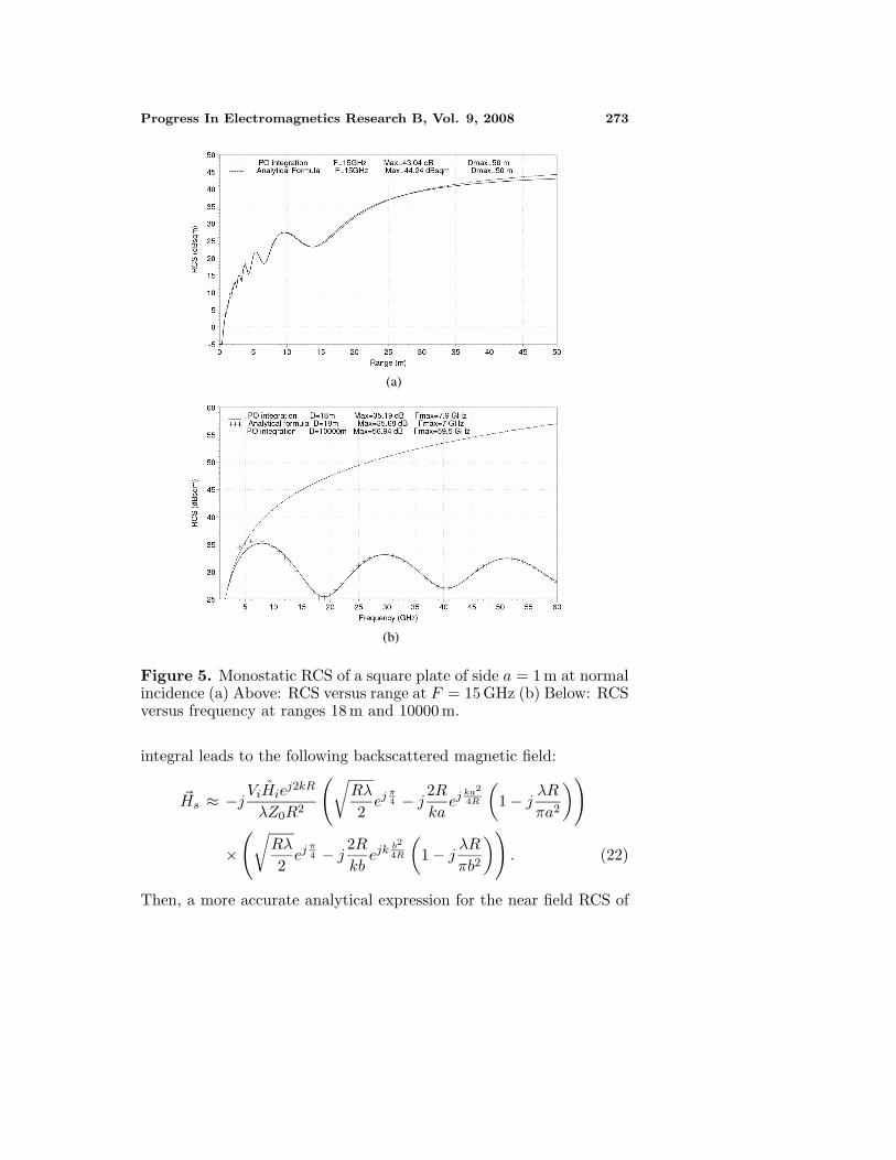
Figure 5 allows analyzing the validity of the simple formula (17).Figure 5(a) presents the RCS of a perfectly conducting square

plate of side a = 1 m, versus range R, at 15 GHz, calculated with thePO integral and with the analytical formula (17). Figure 5(b) showsthe RCS of the same target versus frequency at R = 18 m, calculatedusing the PO integral and using (17), then at R = 10000 m (far field)calculated with PO. In both cases, one notes a good accuracy of theanalytical formula (17) with the following restrictions:- When the range becomes important, the RCS calculated with theanalytical relation diverges from the PO integration result. Numericalcomputations show that to obtain RCS accuracy better than 1 dB with(17) it is necessary to verify the criterion:

R < 0.0932π2a2

λ. (21)

When the frequency becomes low (below 5GHz), the RCS calculatedwith the analytical relation diverges also from the PO integrationresult.

These upper and lower bounds of validity isversus range andfrequency are due to the fact that (17) has been established consideringonly the first term of the asymptotic expansion of the Fresnelintegral (B7) which appears when the magnetic field expression (15) isdeveloped using the stationary phase method [10]. This approximationis only valid for large arguments of the Fresnel integral; but whenthe range becomes large, or when the frequency becomes low, thisargument becomes small and it’s necessary to keep other terms.Keeping the two first terms of the asymptotic expansion of the Fresnel


(a)

(b)

Figure 5. Monostatic RCS of a square plate of side a = 1 m at normalincidence (a) Above: RCS versus range at F = 15 GHz (b) Below: RCSversus frequency at ranges 18 m and 10000 m.

integral leads to the following backscattered magnetic field:

�Hs ≈ −j ViHiej2kR

λZ0R2

(√Rλ

2ej π

4 − j2Rka

ej ka2

4R

(1 − j

λR

πa2

))

×(√

Rλ

2ej π

4 − j2Rkb

ejk b2

4R

(1 − j

λR

πb2

)). (22)

Then, a more accurate analytical expression for the near field RCS of


Figure 6a. Monostatic RCS of a square plate of side 1 m at normalincidence, versus range at F = 15 GHz — PO integration in solid line— formula (23) in dashed line.

5 10 15 20 25 30 35 40Frequency (GHz)

40

35

30

25

20

RC

S (

dBsq

m)

.... PO integration D=18m Max=35.19 dB Fmax=7.9 GH+++ Analytical formula D=18m Max=35.68 dBsqm Fmax=7 GH____ Analytical formula with more terms D=18m Max=35.55 dBsqm Fmax=8 GH

Figure 6b. Monostatic RCS of a square plate of side 1 m at normalincidence versus frequency at 18 m — PO integration in dashed line —formula (17) in cross — formula (23) in solid line.

the rectangular plate is obtained using (22) and (4)

σ ≈ 4πλ2

∣∣∣∣∣(√

Rλ

2ej π

4 − j2Rka

ej ka2

4R

(1 − j

λR

πa2

))

×(√

Rλ

2ej π

4 − j2Rkb

ejk b2

4R

(1 − j

λR

πb2

))∣∣∣∣∣2

(23)


Figure 6a presents the RCS of a perfectly conducting square plate ofside a = b = 1 m versus range R at 15 GHz, calculated with the POintegral and also with the analytical formula (23). One observes asignificant reduction of the error; now the criterion (21) gives RCSaccuracy better than 0.3 dB.- Numerical computations, with (17) and (23), show an error inferior to1 dB as R becomes greater than three times the target size. This lowerbound of validity versus R is mainly due to the phase and amplitudeapproximations (7). So, it is almost the same for the plate and thedisc. Therefore, these results can be enhanced if the amplitude andphase approximations (7) are limited.

4. CONCLUSION

A method based on Physical Optics has been developed to calculate thenear-field RCS of targets in the high frequency limit. Then, analyticalrelations have been established to approximate the monostatic near-field RCS of circular and square flat metallic plates observed in normalincidence. Some validity domains and asymptotic limits are establishedfor these formulae. These new expressions demonstrate the remarkablephenomena already underlined in [6, 7], as the periodic behavior versusfrequency of the near-field RCS of a metallic circular plate, and alsothe dependence of its maximum RCS which is only function of theobservation range. Future works will focus on finding such analyticalformulae valid in oblique incidence, for flat plates and for other simpleshapes. Also we will try to limit some approximations, done onamplitude and phase terms, in order to enhance the accuracy for verylow ranges.

APPENDIX A.

The magnetic field scattered by an obstacle of surface S is deducedfrom the Magnetic field integral equation (MFIE) [8, 9]

�Hs =14π

∫∫S

(jωε �Mφ+ �J ∧∇′φ+

j

ωµ

[�M · ∇′

]∇′φ

)ds (A1)

with the �M = �E ∧ n and �J = n ∧ �H the magnetic and electriccurrents induced on S, and with the total EM fields �E = �Ei + �Es

and �H = �Hi + �Hs, where { �Ei, �Hi} and { �Es, �Hs} are respectively theincident and scattered EM fields.


φ = ejkr

r is the Green function and its gradient

∇′φ = −∇φ = −(jk − 1

r

)· r (A2)

Using the relation [�L · ∇′]∇′φ = ∇′[�L · ∇′φ], one shows that[(�J

�M

)· ∇′

]∇′φ=

[−(1 − jkr)

(�J

�M

)+(3−j3kr−k2r2)

{r ·

(�J

�M

)}r

]φ

r2

(A3)

Then, replacing (A2) and (A3) in (A1), one obtains

�Hs =j

4πωµ

∫∫S

[(−1 + jkr + k2r2) �M − (k2r2 + jkr)Z �J ∧ r

+ (3 − j3kr − k2r2)(r · �M)r] φ

r2ds (A4)

Considering the surface S is such that its radii of curvature at allpoints are much larger than the wavelength [9], it allows approximatingit at any point as an infinite plane tangent to the surface at thatpoint. Moreover, if S is perfectly electric conducting, the magneticand electric currents induced on S are

�J = 2n ∧ �Hi (A5)�M = 0 (A6)

Putting (A5) and (A6) in (A4) leads to

�Hs ≈−j

2πωµ

∫∫S

[(k2r2 + jkr)Z0(n ∧ Hi) ∧ r

] φ

r2ds (A7)

and supposing kr � 1 allows to write

�Hs ≈−jλ

∫∫S

[(�n ∧ Hi) ∧ r

]φds (A8)

The incident magnetic field can be expressed

�Hi =Vi

Z0

ejkr

rhi (A9)

with Vi the generator voltage.Finally, substituting (A9) in (A8) and using the vectorial identity

(a ∧ b) ∧ c = (c · a)b− (c · b)a lead to

�Hs ≈ −j Vi

λZ0

∫∫S

[(r · n)hi − (r · hi)n

] ej2kr

r2ds (A10)


APPENDIX B.

We need to solve an integral of the form

I =∫ b2

b1

f(x)ejkg(x)dx (B1)

where f(x) = 1, g(x) = x2/R, b1 = −a/2 and b2 = a/2.The stationary phase approximation [10] allows expressing this

integral as

I = I0 − 2Ia/2 (B2)

with

I0 =

√2π

k|g′′(x0)|f(x0) exp

{j[kg(x0) +

π

4sgn(g′′(x0))

]}(B3)

Ia/2 = U(−ε)I0 + εf(a/2) exp{jkg(a/2) ∓ jv2

}×

√2

k|g′′(a/2)|F ∓ (v){g′′(α)

> 0< 0

}(B4)

where x0 is a first order stationary phase point defined by g′(x0) =0 and g′′(x0) �= 0: Here x0 = 0. ε = sgn(a/2 − x0), v =√

k2|g′′(a/2)| |g′(a/2)| and U(x) is the unit step function, i.e., U = 1

for x ≥ 0 and zero otherwise.F±(x) =

∫ ∞x e±jt2dt is the Fresnel integral defined for real

arguments,We have g(x0) = g′(x0) = 0, g′′(x0) = 2/R, g(a/2) =

a2/4R, g′(a/2) = a/R, g′′(a/2) = 2/R, v =√

ka2

4R , which give

I0 =

√Rλ

2kej π

4 (B5)

Ia/2 =

√R

kF ±

(√ka2

4R

)(B6)

For large arguments of the Fresnel integral, its asymptotic expansionis

F±(x) ≈ 12x

exp{±j

(x2 +

π

2

)} ∞∑m=0

j∓m

(12

)m

x−2m (B7)


where (12

)0

= 1,(

12

)m

=12

(12

+ 1)· · ·

(12

+m− 1)

Substituting the Fresnel integral by its asymptotic expansion in (B6),we get

Ia/2 =

√R

k

1

2

√4Rka2

exp{j

(ka2

4R+π

2

)} ∞∑m=0

j−m

(12

)m

(√ka2

4R

)−2m

(B8)

Then, limiting the asymptotic expansion to the first term (m = 0) andto the second term (m = 1), we find

Im=0a/2 = j

R

kaexp

{j

(ka2

4R

)}(B9a)

Im=1a/2 = j

R

kaexp

{j

(ka2

4R

)} (1 − j

λR

πa2

)(B9b)

Combining (B9a) and (B9a) with (B5) and (B2) gives finally

Im=0 =

√Rλ

2kej π

4 − j2Rka

exp{j

(ka2

4R

)}(B10a)

Im=1 =

√Rλ

2kej π

4 − j2Rka

exp{j

(ka2

4R

)} (1 − j

λR

πa2

)(B10b)

REFERENCES

1. Vogel, M. H., “The physical optics approximation in the near-fieldregion,” report no FEL 1989-100n TNO Physics and ElectronicsLaboratory, March 1989.

2. Legault, S. R. and A. Louie, “Validation and implementation ofa near-field Physical Optics formulation,” Defence R&D CanadaOttawa, Technical Memorandum, DRDC Ottawa TM 2004-131,August 2004.

3. Yu, C. L., R. Kipp, D. J. Andersh, and S. W. Lee, “Near-fieldelectromagnetic modeling and analysis,” IEEE AP-S InternationalSymposium and URSI Radio Science Meeting, Montreal, July 13–18, 1997.


4. Lee, S. W. and S. K. Jeng, “NcPTD 1.2 a high frequency near-fieldRCS computation code based on physical theory of diffraction,”DEMACO, Inc., Champaign, IL, June 1991.

5. Pouliguen, P., P. Gadenne, and J. Y. Marty, “Radar reflectivityof a target illuminated by a spherical wave,” Symposium AGARDsur l’analyse de la Signature Radar et de la Videoscopie des ciblesMilitaires, Ankara Turquie, Octobre 7–10, 1996.

6. Pouliguen, P. and L. Desclos, “A physical optics approach to near-field RCS computations,” Annals of Telecommunications, Vol. 51,Nos. 5–6, 219–226, May–June 1996.

7. Desclos, L. and P. Pouliguen, “The physical optics applied todiscs and square plates in near-fields leads to simple formula,”Microwave and Optical Technology Letters, Vol. 9, No. 5, 278–283,August 1995.

8. Stratton, J. A., Electromagnetic Theory, Mc Graw-Hill BookCompany, Inc., New York, 1947.

9. Ruck, G. T., D. E. Barrick, W. D. Stuart, and C. K. Krichbaum,Radar Cross Section Handbook, Plenum Press, New York, 1970.

10. James, G. L., Geometrical Theory of Diffraction for Electromag-netic Waves, 3rd Edition, Peter Peregrinus Ltd., 1986.

11. Pouliguen, P., R. Hemon, J. Saillard, and J. F. Damiens, “RCScomputation in near-field,” Days on Diffraction, St-Petersburg,May 30–June 2, 2006.

Analytical Formulae for Radar Cross Section of Flat Plates in Near Field and Normal Incidence

Documents

Transcript of Analytical Formulae for Radar Cross Section of Flat Plates in Near Field and Normal Incidence