Analytical and Numerical Modeling of Paraffin Wax in Pipelines - DiVA

Analytical and Numerical Modeling of Paraffin Wax in Pipelines

Marte Stubsjøen

Petroleum Geoscience and Engineering

Supervisor: Jon Steinar Gudmundsson, IPT

Department of Petroleum Engineering and Applied Geophysics

Submission date: June 2013

Norwegian University of Science and Technology

Preface

The presented master thesis is a result of the compulsory subject TPG 4905 Petroleum

production, master thesis conducted at the Department of Petroleum Engineering

and Applied Geophysics at the Norwegian University of Science and Technology

(NTNU) in the spring of 2012 . The study of the numerical wax deposit model was

initiated by Siljuberg (2012), taken one step further by the writer (Stubsjøen, 2013)

and is finally fulfilled with the current work.

I want to thank my supervisor Jon Steinar Gudmundsson for his kind support

throughout the semester, Erlend Vatevik for always fixing whatever computer trou-

ble I would meet, and Ole Martin Brende for being available whenever I would need

him.

i

Abstract

Paraffin wax deposition, or the settling of solid wax particles on pipelines

and equipment, is an extensive problem encountered in oil production and

transportation. Flowing through subsea pipelines, oil and condensate are sub-

ject to cooling. If the temperature of a supersaturated crude oil mixture drops

below the solubility limit of wax, known as the wax appearance temperature

(WAT), solid paraffin start to appear in solution. Assuming temperatures

below the WAT and a radial heat flux from the fluid to the surroundings,

paraffin will precipitate, adhere to the inner pipe wall and gradually accumu-

late. The result is an undesirable layer of paraffin wax on the inner pipe wall

causing flow restrictions, reduced production and a need for remediation.

In the current thesis, the applicability of five effective thermal conductivity

models for determination of the effective thermal conductivity of paraffin wax

deposits have been evaluated. Based on the structure of the deposit, the

Effective Medium Theory is found applicable. The influence of the deposit on

the thermal conditions in the pipeline has been examined, and the temperature

at the deposit surface is found to increase with an increasing wax deposit

thickness. The increased temperature at the oil/deposit interface reduces the

radial temperature gradient in the pipeline, being the thermal driving force

for deposition. The result is a reduced growth rate of the wax layer with

time and a need for dynamic simulations to avoid over prediction of the wax

deposit thickness.

The most important part of the presented work, is the implementation of

an analytical and a numerical model facilitating wax deposit predictions. Sim-

ulations have been conducted on a typical subsea pipeline and the results have

been compared. The analytical model, with its assumption of thermodynamic

equilibrium between the solubility of wax and the actual wax concentration

at ever point in the pipeline, has shown to yield a significantly higher amount

of wax to be expected, compared to the results obtained by the numerical

model, taking the precipitation kinetics of wax into account.

ii

Sammendrag

Avsetning av parafiner i forbindelse med produksjon og transport av olje er et ut-

bredt problem i petroleumsindustrien. Nar olje og kondensater strømmer gjennom

undervannsrørledninger fra reservoaret til produksjonsfasilitetene, utsettes fluidet

for kjøling. Dersom temperaturen i rørledningen faller under løselighetsgrensa for

voks, vil utfelling av parafiner i fast form inntreffe. Med temperaturer i røret un-

der voksutfellingsgrensa og en radiell varmestrømning fra fluidet til omgivelsene,

vil parafiner felles ut av raoljen og avsettes pa den indre rørveggen. Resultatet

er et uønsket lag av parafiner som skaper restriksjoner for strømning eller, i verste

fall, blokkerer røret fullstendig med redusert produksjon eller produksjonsstans som

følge.

Fem modeller som beregner den effektive termiske ledningsevnen til to-komponent

systemer har blitt undersøkt i den presenterte oppgaven for a kunne modellere den

termiske ledningsevnen til voksavsetningen. Basert pa avsetningens struktur er ”the

Effective Medium Theory” funnet anvendbar og blitt implementert i de senere vok-

savsetningsmodellene. Voksavsetningens innflytelse pa de termiske forholdende i

rørledningen har blitt undersøkt, og en økende tykkelse av vokslaget er funnet a gi

en økt temperatur pa overflaten av voksavsetningen. Som en konsekvens av den økte

temperaturen pa voksavsetningsens overflate, vil den radielle temperaturgradienten,

kjent som den termiske drivkraften for avsetning, avta med en økende vokstykkelsen.

Resultatet er en avtagende vekstrate med tid og en pakrevd dynamisk modellering

dersom en overestimering av vokslagets tykkelse skal unngas.

Undersøkelsene ovenfor leder frem til oppgavens hovedformal; en implemen-

tasjon av en analytisk og en numerisk voksavsetningsmodell med en pafølgende

sammenligning av simuleringsresultater. Den analytiske modellen baserer seg pa

termodynamisk likevekt der det antas at vokskonsentrasjonen følger løseligheten

i ethvert punkt i rørledningen, mens den numeriske modellen inkluderer en ”pre-

cipitation rate constant” som tar hensyn til avviket mellom løselighet og faktisk

konsentrasjon som kan oppsta ved turbulent strømning. Basert pa litteraturstudiet

og prinsippet beskrevet, var den analytiske modellen forventet a gi en større vok-

savsetningstykkelse enn de numeriske simuleringene. Dette ble bekreftet ved en

sammenligning av de analytiske og numeriske resultatene. For de simulerte forhold-

ene ga den analytiske modellen etter et døgn en maksimal voksavsetningstykkelse

som var 3.1 mm høyere enn den numeriske modellen og etter en uke var forskjell pa

15.8 mm.

iii

Contents

List of Figures viii

List of Tables ix

1 Introduction 1

1.1 The Problem of Wax Deposition . . . . . . . . . . . . . . . . . . . . . 1

1.2 Field Development . . . . . . . . . . . . . . . . . . . . . . . . . . . . 1

1.3 Current Work . . . . . . . . . . . . . . . . . . . . . . . . . . . . . . . 2

2 Modeling 3

2.1 Model Classifications . . . . . . . . . . . . . . . . . . . . . . . . . . . 3

2.2 Uncertainty in Modeling . . . . . . . . . . . . . . . . . . . . . . . . . 3

2.3 Programing Language . . . . . . . . . . . . . . . . . . . . . . . . . . 4

3 Transport Phenomena 5

3.1 General Equation . . . . . . . . . . . . . . . . . . . . . . . . . . . . . 5

3.2 Dimensionless Numbers . . . . . . . . . . . . . . . . . . . . . . . . . . 6

3.3 Flow Regimes . . . . . . . . . . . . . . . . . . . . . . . . . . . . . . . 6

3.3.1 Reynolds Number . . . . . . . . . . . . . . . . . . . . . . . . . 6

4 Heat Transfer 8

4.1 Conduction . . . . . . . . . . . . . . . . . . . . . . . . . . . . . . . . 8

4.1.1 Governing Equation . . . . . . . . . . . . . . . . . . . . . . . 8

4.1.2 Conduction Through Cylinders . . . . . . . . . . . . . . . . . 9

4.1.3 Conduction Through Multiple Layers . . . . . . . . . . . . . . 10

4.2 Dimensionless Numbers in Heat Transfer . . . . . . . . . . . . . . . . 11

4.2.1 Nusselt Number . . . . . . . . . . . . . . . . . . . . . . . . . . 11

4.2.2 Prandtl Number . . . . . . . . . . . . . . . . . . . . . . . . . 12

4.3 Fourier’s Law in the Turbulent Flow Regime . . . . . . . . . . . . . . 12

4.4 Convection . . . . . . . . . . . . . . . . . . . . . . . . . . . . . . . . . 13


4.4.2 Convective Heat Transfer Coefficient . . . . . . . . . . . . . . 14

4.5 Heat Transfer in Oil Flowing Pipelines . . . . . . . . . . . . . . . . . 14

5 Mass Transfer 16

5.1 Diffusion . . . . . . . . . . . . . . . . . . . . . . . . . . . . . . . . . . 16


5.2 Dimensionless Numbers in Mass Transfer . . . . . . . . . . . . . . . . 16

5.2.1 Schmidt Number . . . . . . . . . . . . . . . . . . . . . . . . . 17

iv

5.2.2 Sherwood Number . . . . . . . . . . . . . . . . . . . . . . . . 17

5.3 Fick’s Law in the Turbulent Flow Regime . . . . . . . . . . . . . . . 17

6 Paraffin Wax 19

6.1 Chemistry of Wax . . . . . . . . . . . . . . . . . . . . . . . . . . . . . 19

6.2 Wax Appearance . . . . . . . . . . . . . . . . . . . . . . . . . . . . . 19

6.3 Deposit Formation . . . . . . . . . . . . . . . . . . . . . . . . . . . . 20

6.4 Wax Handling . . . . . . . . . . . . . . . . . . . . . . . . . . . . . . . 21

7 Literature 22

7.1 Wax Deposition Mechanisms . . . . . . . . . . . . . . . . . . . . . . . 22

7.2 Wax Deposition Modeling . . . . . . . . . . . . . . . . . . . . . . . . 22

7.2.1 Analytical Model . . . . . . . . . . . . . . . . . . . . . . . . . 23

7.2.2 Numerical Model . . . . . . . . . . . . . . . . . . . . . . . . . 23

8 Effective Thermal Conductivity of Two Component Systems 25

8.1 Thermal Conductivity . . . . . . . . . . . . . . . . . . . . . . . . . . 25

8.2 Stratified Models . . . . . . . . . . . . . . . . . . . . . . . . . . . . . 26

8.3 Maxwell-Eucken Model . . . . . . . . . . . . . . . . . . . . . . . . . . 26

8.3.1 Maxwell-Eucken 1 . . . . . . . . . . . . . . . . . . . . . . . . . 26

8.3.2 Maxwell-Eucken 2 . . . . . . . . . . . . . . . . . . . . . . . . . 27

8.4 Effective Medium Theory . . . . . . . . . . . . . . . . . . . . . . . . . 27

8.5 Evaluation of Model Applicability . . . . . . . . . . . . . . . . . . . . 28

8.6 Application of Models . . . . . . . . . . . . . . . . . . . . . . . . . . 29

9 Interface Temperatures 31

9.1 Thermal Resistance for Conduction and Convection . . . . . . . . . . 31

9.2 Situation in the Oil Pipeline . . . . . . . . . . . . . . . . . . . . . . . 32

9.3 Temperature Calculations . . . . . . . . . . . . . . . . . . . . . . . . 33

9.4 Influence of the Wax Deposit . . . . . . . . . . . . . . . . . . . . . . 34

9.4.1 Influence of Deposit Thickness . . . . . . . . . . . . . . . . . . 34

9.4.1.1 Results . . . . . . . . . . . . . . . . . . . . . . . . . 34

9.4.2 Influence of Wax Fraction . . . . . . . . . . . . . . . . . . . . 36

9.4.2.1 Results . . . . . . . . . . . . . . . . . . . . . . . . . 36

9.4.3 Discussion . . . . . . . . . . . . . . . . . . . . . . . . . . . . . 37

10 Analytical Modeling 39

10.1 Application and Assumptions . . . . . . . . . . . . . . . . . . . . . . 39

10.2 Flow Regions . . . . . . . . . . . . . . . . . . . . . . . . . . . . . . . 39

10.3 Temperature Calculations . . . . . . . . . . . . . . . . . . . . . . . . 40

v

10.3.1 Average Bulk Flow Temperature . . . . . . . . . . . . . . . . 41

10.3.2 Boundary Layer Temperature . . . . . . . . . . . . . . . . . . 41

10.3.3 Interface Temperatures . . . . . . . . . . . . . . . . . . . . . . 42

10.4 Wax Deposit Calculations . . . . . . . . . . . . . . . . . . . . . . . . 42

10.5 Simulations . . . . . . . . . . . . . . . . . . . . . . . . . . . . . . . . 43

10.5.1 Results . . . . . . . . . . . . . . . . . . . . . . . . . . . . . . . 43

11 Numerical Modeling 46

11.1 Application and Assumptions . . . . . . . . . . . . . . . . . . . . . . 46

11.2 Mathematical Approach . . . . . . . . . . . . . . . . . . . . . . . . . 46

11.2.1 Continuity Equations . . . . . . . . . . . . . . . . . . . . . . . 47

11.2.2 Continuity Equations on a Finite-Difference Form . . . . . . . 48

11.2.3 Finite-Difference Solution . . . . . . . . . . . . . . . . . . . . 48

11.3 Numerical Calculations . . . . . . . . . . . . . . . . . . . . . . . . . . 49

11.3.1 Heat Transfer Calculations . . . . . . . . . . . . . . . . . . . . 49

11.3.2 Mass Transfer Calculations . . . . . . . . . . . . . . . . . . . . 51

11.4 Boundary Conditions . . . . . . . . . . . . . . . . . . . . . . . . . . . 53

11.5 Wax Deposit Calculations . . . . . . . . . . . . . . . . . . . . . . . . 53

11.6 Numerical Simulations . . . . . . . . . . . . . . . . . . . . . . . . . . 55

11.6.1 Results . . . . . . . . . . . . . . . . . . . . . . . . . . . . . . . 55

12 Model Comparison 58

12.1 External Material for Comparison . . . . . . . . . . . . . . . . . . . . 58

12.2 Comparison of Results . . . . . . . . . . . . . . . . . . . . . . . . . . 59

13 Shortcomings 62

13.1 Shortcomings in the Implemented Models . . . . . . . . . . . . . . . . 62

13.2 Shortcomings in the Conducted Work . . . . . . . . . . . . . . . . . . 62

14 Summary 64

15 Future Work 66

A References 67

B Heat Transfer Coefficient 71

B.1 Chilton-Colburn Correlation . . . . . . . . . . . . . . . . . . . . . . . 71

B.2 Dittus-Boelter Correlation . . . . . . . . . . . . . . . . . . . . . . . . 71

B.3 Pethukov Correlation . . . . . . . . . . . . . . . . . . . . . . . . . . . 72

B.4 Gnielski Correlation . . . . . . . . . . . . . . . . . . . . . . . . . . . 72

vi

C Diffusion Coefficient 74

D Precipitation Rate Constant 75

E Applied Solubility Function 77

F Simulation Input 78

G Effective Thermal Conductivity Models 80

H Heat Resistance Contribution 81

I Temperature Profiles 85

J Analytical Solution 88

K Numerical Solution 93

L MATLAB I Effective Thermal Conductivity Calculations 95

M MATLAB II Thermal Resistance 97

N MATLAB III Interface Temperatures 100

O MATLAB IV Analytical Wax Deposit Model 103

P MATLAB Numerical Wax Deposit Model 109

vii

List of Figures

4.1 Radial Heat Flow . . . . . . . . . . . . . . . . . . . . . . . . . . . . . 14

6.1 Wax Deposition . . . . . . . . . . . . . . . . . . . . . . . . . . . . . . 21

8.1 Microscope Observation of Wax Deposit . . . . . . . . . . . . . . . . 28

8.2 Effective Thermal Conductivity Models Applied on Wax Deposit . . . 29

10.1 Analytical Wax Deposit Profile . . . . . . . . . . . . . . . . . . . . . 44

11.1 Numerical Wax Deposit Profile . . . . . . . . . . . . . . . . . . . . . 56

12.1 Wax Deposit Profile by Commercial Software . . . . . . . . . . . . . 61

G.1 Effective Thermal Conductivity Models . . . . . . . . . . . . . . . . . 80

H.1 Influence of Wax Deposition on Inner Thermal Resistance . . . . . . 81

H.2 Influence of Wax Deposition on Thermal Resistance of Deposit . . . . 82

H.3 Influence of Wax Deposition on Thermal Resistance of Pipe . . . . . 83

H.4 Influence of Wax Deposition on Outer Thermal Resistance . . . . . . 84

I.1 Influence of Wax Deposition on Deposit Surface Temperature . . . . . 85

I.2 Influence of Wax Deposition on Inner Wall Temperature . . . . . . . 86

I.3 Influence of Wax Deposition on Outer Wall Temperature . . . . . . . 87

J.1 Initial Temperature in Bulk Flow and Viscous Sub-layer . . . . . . . 88

J.2 Initial Temperature at Inner and Outer Pipe Wall . . . . . . . . . . . 89

J.3 Inner and Outer Pipe Wall Temperature after 24 hours. . . . . . . . . 90

J.4 Temperature Difference Across Viscous Sub-layer . . . . . . . . . . . 91

J.5 Temperature at Deposit Surface after 1, 2 and 7 days . . . . . . . . . 92

K.1 Radial and Lateral Temperature Profile in Pipeline after 24 hours . . 93

K.2 Radial and Lateral Concentration Profile in Pipeline after 24 hours . 94

viii

List of Tables

1 Latin and Greek Symbols . . . . . . . . . . . . . . . . . . . . . . . . x

2 Dimensionless Numbers . . . . . . . . . . . . . . . . . . . . . . . . . . xiii

3 Acronyms and Abbreviations . . . . . . . . . . . . . . . . . . . . . . xiii

4 Thermal Conductivity Values . . . . . . . . . . . . . . . . . . . . . . 25

5 Effective Thermal Conductivity . . . . . . . . . . . . . . . . . . . . . 30

6 Influence of Deposit Thickness on Thermal Resistance . . . . . . . . . 35

7 Influence of Deposit Thickness on Interface Temperature . . . . . . . 35

8 Influence of Wax Content on Thermal Resistance . . . . . . . . . . . 36

9 Influence of Wax Content on Interface Temperature . . . . . . . . . . 37

10 Deposit Surface Temperature Variations . . . . . . . . . . . . . . . . 38

11 Deposit Thickness by Analytical Model . . . . . . . . . . . . . . . . . 44

12 Deposit Thickness by Numerical Model . . . . . . . . . . . . . . . . . 57

13 Comparison of Numerical Model to External Results . . . . . . . . . 59

14 Comparison of Analytical Model to External Result . . . . . . . . . . 60

15 Numerical versus Analytical Results . . . . . . . . . . . . . . . . . . . 60

16 Comparison of Numerical Model to Commercial Software . . . . . . . 61

17 Input Variables . . . . . . . . . . . . . . . . . . . . . . . . . . . . . . 78

18 Calculated Variables . . . . . . . . . . . . . . . . . . . . . . . . . . . 79

ix

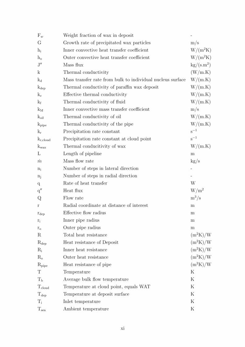
Nomenclature

Table 1: Latin and greek symbols applied.

Latin Symbols Unit

Ai Solid/liquid interface area m2

Alm Logarithmic mean area m2

Alm, deposit Logarithmic mean area of the deposit m2

Alm, pipe Logarithmic mean area of the pipe m2

Ap Surface area of nucleus m2

Awi Area of inner pipe wall m2

Awo Area of outer pipe wall m2

ACj Coefficient for numerical concentration calculations s−1

ATj Coefficient for numerical temperature calculations s−1

BCj Coefficient for numerical concentration calculations s−1

BTj Coefficient for numerical temperature calculations s−1

C Concentration of wax dissolved in solution wt-%

Cb Concentration of wax in the bulk flow wt-%

CCj Coefficient for numerical concentration calculations s−1

CTj Coefficient for numerical temperature calculations s−1

Cp Spesific heat capacity of oil J/(kg.K)

Cwall Concentration of wax in the near-wall region wt-%

CWAT Maximum concentration of wax in oil wt-%

C1 Eddy viscosity correlation constant -

C2 Eddy viscosity correlation constan -

d Inner pipe diameter m

dp Diameter of nucleus m

DAB Binary diffusion coefficient of solute A in solvent B m2/s

Dwo Binary diffusion coefficient of wax in oil m2/sdCdr

Concentration gradient wt-%/mdmdt

Mass deposit rate of wax in oil at liquid/solid interface kg/sdTdr

Temperature gradient K/mdV +

z

dy+ Temperature gradient K/m

Deff Effective binary diffusion coefficient m2/s

DCj Coefficient for numerical concentration calculations s−1

DTj Coefficient for numerical temperature calculations s−1

EA Activation energy J/mol

f Friction factor -

x

Fw Weight fraction of wax in deposit -

G Growth rate of precipitated wax particles m/s

hi Inner convective heat transfer coefficient W/(m2K)

ho Outer convective heat transfer coefficient W/(m2K)

J′′ Mass flux kg/(s.m2)

k Thermal conductivity (W/m.K)

kd Mass transfer rate from bulk to individual nucleus surface W/(m.K)

kdep Thermal conductivity of paraffin wax deposit W/(m.K)

ke Effective thermal conductivity W/(m.K)

kf Thermal conductivity of fluid W/(m.K)

kM Inner convective mass transfer coefficient m/s

koil Thermal conductivity of oil W/(m.K)

kpipe Thermal conductivity of the pipe W/(m.K)

kr Precipitation rate constant s−1

kr,cloud Precipitation rate constant at cloud point s−1

kwax Thermal conducitivity of wax W/(m.K)

L Length of pipeline m

m Mass flow rate kg/s

ni Number of steps in lateral direction -

nj Number of steps in radial direction -

q Rate of heat transfer W

q′′ Heat flux W/m2

Q Flow rate m3/s

r Radial coordinate at distance of interest m

rdep Effective flow radius m

ri Inner pipe radius m

ro Outer pipe radius m

R Total heat resistance (m2K)/W

Rdep Heat resistance of Deposit (m2K)/W

Ri Inner heat resistance (m2K)/W

Ro Outer heat resistance (m2K)/W

Rpipe Heat resistance of pipe (m2K)/W

T Temperature K

Tb Average bulk flow temperature K

Tcloud Temperature at cloud point, equals WAT K

Tdep Temperature at deposit surface K

Ti Inlet temperature K

Tsea Ambient temperature K

xi

Twi Temperature at inner pipe wall K

Two Temperature at outer pipe wall K

Tw+ Dimensionless wall temperature K

T∞ Fluid temperature K

U Overall heat transfer coefficient W/(m2K)

u Average fluid flow velocity m/s

uτ Friction velocity m/s

uz Fluid velocity in lateral direction m/s

v Volume fraction -

Va Molecular volume cm3/mol

Vz Axial velocity m/s

V+z Dimensionless turbulent velocity -

y Distance from inner pipe wall m

yτ Friction distance m

y+z Dimensionless distance from inner pipe wall -

z Axial distance m

Greek Symbols Unit

αT Thermal diffusivity m2/s

αtot Total thermal diffusivity m2/s

β Constant for heat of fusion crystallization -

∆r Grid size in radial direction m

∆rwall Wall thickness m

δ Deposit thickness m

ε Eddy diffusivity m2/s

εh Turbulent heat diffusivity m2/s

εm Turbulent mass diffusivity m2/s

γ Dimensionless function of molar volume -

µcloud Dynamic viscosity of oil at WAT Pa.s

µoil Dynamic viscosity of oil Pa.s

νoil Kinematic viscosity of oil m2/s

ρoil Density of oil kg/m3

ρwax Density of wax kg/m3

ρn Number density of nucleus 1/m3

τw Wall shear stress Pa

xii

Table 2: Dimensionless Numbers.

Symbol Number Definition

Re Reynolds Number udν

Pr Prandtl Number cpµ

k= ν

α

PrT Turbulent Analogy to the Prandtl Number εεh

Nu Nusselt Number hdkf

Sc Schmidt Number νDAB

ScT Turbulent Analogy to the Schmidt Number εεm

Sh Sherwood Number kMdDwo

Shp Sherwood Number for Micro Particles kddpDwo

Table 3: Acronyms and Abbreviations.

Abbreviation Description

CPM Cross Polar Microscopy

DSC Differential Scanning Calorimetry

FTIR Fourier Transform Infrared Spectoscopy

HRD Heat Resistance Distribution

HTGC High Temperature Gas Chromatography

MATLAB Matrix Laboratory

NMR Nuclear Magnetic Resoncance

OPEX Operational Expenditure

WAT Wax Apperance Temperature

WPC Wax Precipitation Curve

xiii

1 Introduction

As oil production is moving further offshore to colder regions and greater depths,

the oil industry is facing increasing challenges in the area of flow assurance. One of

the problems arising when tempting to ensure an economically feasible flow of hy-

drocarbons from the reservoir well bore to the treatment facilities, is the deposition

of high molecular weight paraffins at the inner pipe wall, a topic to be presented

below.

1.1 The Problem of Wax Deposition

The solubility of paraffins, interchangeably referred to as wax or paraffin wax, is

temperature dependent, decreasing with decreasing temperature. At typical reser-

voir conditions1, the wax molecules are kept dissolved in the oil. Flowing through

the subsea pipeline resting on the ocean floor, the waxy crude looses heat to the

colder surroundings and a radial temperature gradient over the cross-sectional area

of the pipe is established.

If the temperature of a supersaturated wax-oil mixture drops below the wax

appearance temperature (WAT), also known as the cloud point, solid wax molecules

start to appear in solution. Assuming the existence of a radial temperature gradient,

the precipitated wax will deposit on the inner pipe wall, causing flow restrictions or,

in worst case, plugs the pipeline entirely. The result is a need for intervention and

a possible shut-down of production (Huang, 2011).

1.2 Field Development

In 2012, there were more than 8500 km subsea export pipelines and 3000 km subsea

infield flow lines at the Norwegian continental shelf. Out of these, almost 1000 km of

the export lines were oil flowing and a substantial fraction of the produced and trans-

ported fluids were oils and gas condensates containing paraffin waxes (Rønningsen,

2012). On a global basis, waxy crudes have been estimated to represent about 20%

of the petroleum reserves produced and pipelined, making prediction of wax deposits

a relevant area for the petroleum industry (Frigaard et al., 2007).

Deposition of wax is recognized as a complex process involving a number of

disciplines, among those flow dynamics, fluid chemistry, precipitation kinetics (crys-

tal growth) and thermodynamics (Rønningsen, 2012). Currently there is no good

method available for detection of wax deposits in oil flowing pipelines; When the

pressure drop in a pipeline system has increased noticeably, the problem is already

1Typical off-shore reservoir conditions are temperatures between 70-150◦C and pressure in therange of 55-100 MPa (Singh et al., 2000).

1

severe (Schulkes, 2013). Without any satisfying methods for detection available,

mathematical modeling is a valid option for wax deposit prediction and what is

applied in the industry.

Running wax deposit simulations, the aim is to be able to predict whether de-

position should be expected or not, where in the pipeline accumulation of paraffin

wax might occur and how fast the potential situation will progress. The simulators

are meant to serve as a tool to support project decisions related to wax deposition,

including planning of thermal insulation, pigging intervals and other remediation

techniques to be applied.

Handling of wax deposits is an expensive affaire, adding significant costs to the

operational expenditure (OPEX). Addressing the problem of deposition at an early

stage of a field development project, may reduce the overall cost of the field. Apply-

ing insulation to prevent deposit formation in the first place may reducing or avoide

loss of system capacity and the use of expensive chemical injection (Leontaritis et

al., 2003).

1.3 Current Work

The aim of the current work, is to implement an analytical and a numerical model

for prediction of paraffin wax deposits on the wall of a typical subsea oil flowing

pipeline. If the applicability of the models is not be limited to flow loops, where

the temperature at the pipe wall can be kept artificially constant, calculations of a

varying wall temperature throughout the pipeline is required.

To gain knowledge and insight into the phenomena of heat and mass transfer,

a theoretical study will have to be conducted. The aim of the study is to be able

to mathematically derive and construct the wax deposit models and implement the

results in the chosen computer language. Assuming a successfully implementation of

the models, the final objective is to run simulations for comparison of the predicted

wax deposit thicknesses when the same fluid under the same flow conditions has

been applied. This will allow for quantification of the deviation between the results

obtained by the two models that will occur, if any.

2

2 Modeling

A simulator is a mathematical model or computer code imitating a real-world system

(O’Hagan, 2006). The aim of a simulator is to be able to predict the responses of a

system over time. To execute the simulations, a mathematical model based upon the

physical processes of the system in question will have to be developed. The model

represents the system to be examined and the simulations imitates what takes place

within the system.

2.1 Model Classifications

A simulator can be built as a probabilistic or a deterministic model. In a proba-

bilistic model, randomness is present and the outcome is a probability distribution

(O’Hagan, 2006). A probabilistic model provides a structured approach to account

for uncertainty and is frequently applied in the area of economy. A deterministic

model produces the same output values every time, if given the same input, and can

be regarded a mathematical function taking in a vector x (input values) resulting

in an output vector y = f(x) (O’Hagan, 2006).

Simulators can be further divided into static and dynamic models. In a static

model, the conditions of a system does not change with time, that is, steady state

is assumed. In a dynamic model, on the other hand, the evolving behavior of a

system is described. The changes in conditions, accounted for in a dynamic model,

results in a more complex and computational expensive model (O’Hagan, 2006). As

a result, the calculations of a dynamic model will have to be iterative, that is, at

each time step the dynamic model takes in the current state vector as parts of its

input and produces an updated vector to be used in the next step.

Since there is no randomness involved in the modeled wax deposition process, the

analytical and numerical wax deposit models are both deterministic. As the static

models are less computational expensive than the dynamic models, static simulations

are preferred if the situation allows for it. The need for dynamic simulations in the

current work will be evaluated in Chapter 9.

2.2 Uncertainty in Modeling

In every model there is uncertainty regarding how close the outcome of the simula-

tions are to the actual real-world values. This uncertainty is related to the accuracy

of the input values and the correctness of the model, that is, if the mathematical

model is a valid description of the actual conditions of the system (O’Hagan, 2006).

One way to gain knowledge about the uncertainty of a model, is to perform

a sensitivity analysis. The idea of a sensitivity analysis is to characterize how the

3

simulation outputs responds to a change in the input values (Kennedy and O’Hagan,

2001). Identifying which inputs the result is relatively sensitive, or insensitive, to

provides knowledge about which inputs one should pay extra close attention to. For

the purpose of uncertainty reduction, a sensitivity analysis on the implemented wax

deposit models will be recommended as part of a future work.

2.3 Programing Language

The wax deposit models have been implemented in MATLAB. MATLAB is an

acronym for Matrix Laboratory and a software widely used among engineers and

scientist in industry and academia (MathWorks, 2013). The program can be used

for development of algorithms, creation of models, numerical calculations and visu-

alization.

The main advantage of using MATLAB, compared to spreadsheets or traditional

programming languages, is the tools and built-in math functions (MathWorks, 2013).

The language was found suitable for the current work because of its flexibility and

ease of use.

4

3 Transport Phenomena

The overall behavior of paraffin wax in pipelines can be described theoretically by

heat, mass and momentum equations. As the transport phenomena can be charac-

terized by the same type of general equation, the processes are often considered as

one discipline (Geankoplis, 2003). Momentum transfer, or fluid mechanics is divided

into two branches; fluid statics and fluid dynamics. The former is dealing with flu-

ids at rest, whilst the latter applies to fluids in motion. In the current thesis, fluid

dynamics is utilized when calculating the temperature and concentration profiles of

the numerical solution. The main focus will, however, be at the principles of heat

and mass transfer as these are the governing mechanisms.

3.1 General Equation

The general transport equation describes the rate of transfer for any of the three

transport processes and can be written as (Geankoplis, 2003):

Rate of Transfer =Driving Force

Resistance(3.1)

or mathematically:

Ψz = −δ dΓ

dz(3.2)

where Ψz (amount of property/s.m2) is the flux of the property defined as amount of

property being transferred per unit time per unit cross-sectional area perpendicular

to the z direction of flow, δ (m2/s) is a proportionality constant termed diffusivity,

Γ (property/m3) is the concentration of property, and z (m) is the distance in the

transport direction.

Integrating and rearranging Equation (3.2), results in a general expression for

the flux of the property is obtained:

Ψz

z2∫z1

dz = −δΓ2∫

Γ1

dΓ (3.3)

Ψz =δ(Γ1 − Γ2)

z2 − z1

(3.4)

The transport equation is in heat and mass transfer known as Fourier’s law and

Fick’s law, respectively, and will be presented in the succeeding chapters.

5

3.2 Dimensionless Numbers

A dimensionless number is a quantity with no physical dimension associated with

it. It is widely used in mathematics and physics and also familiar from every-

day life (counting). Dimensionless numbers are often expressed as ratios of non-

dimensionless quantities, as are the case in the current thesis. When two or more

processes can be expressed by dimensionless equations of the same form, they are

referred to as analogous (Incropera et al., 2011).

Two pair of analog dimensionless numbers have been applied in the current

work. The Prandtl number in heat transfer is analog to the Schmidt number in

mass transfer, and the Nusselt number in heat transfer to the Sherwood number in

mass transfer. Additionally, the Reynolds number (Re) from momentum transfer

has been used.

3.3 Flow Regimes

Fluid flow can be divided into two flow regimes; laminar and turbulent flow. In the

laminar flow regime, the movement of the fluid is highly ordered and streamlines at

which the fluid particles move along can be identified. Under turbulent flow condi-

tions, the fluid movement is highly irregular and velocity fluctuations characterizes

the flow. The fluctuations in turbulent flow affects the transfer processes, increasing

the rate of transfer in the fluid (White, 2008).

3.3.1 Reynolds Number

The Reynolds number (Re) is a dimensionless quantity expressing the ratio of inertia

to viscous forces, defined as (White, 2008):

Re =ρud

µ=ud

ν(3.5)

where ρ (kg/m3) is the fluid density, u (m/s) is the fluid velocity, d (m) is the inner

pipe diameter, µ (kg/m.s) is the dynamic viscosity and ν (m2/s) is the kinematic

viscosity. The kinematic viscosity, defined as (White, 2008):

ν =ρ

µ(3.6)

where ρ (kg/m3) is the fluid density and µ (kg/m.s) the dynamic viscosity as above.

The kinematic viscosity is a transport property in momentum transfer, also referred

to as diffusivity of momentum.

The flow regime in which one are operating in is determined by the value of the

Reynolds number. When the Reynolds number is very low, the effects of inertia

6

are negligible and the fluid motion is viscous (creep). Moderate Reynolds number

indicates laminar flow, whilst high Reynolds numbers implies turbulent conditions

(White, 2008).

In a cylinder, the transition zone between laminar and turbulent flow is found

around the critical Reynolds number Red,crit ≈ 2300 (White, 2008). Below the

critical Reynolds number the flow is laminar and above a breakdown of the laminar

motion causes the flow to become turbulent (White, 2008). Under normal operative

conditions, the flow in oil flowing pipelines, as investigated in the current thesis, will

be turbulent.

7

4 Heat Transfer

Heat transfer, or heat, is defined as thermal energy in transit due to a spatial tem-

perature difference. There are three basic mechanisms of heat transfer; thermal

conduction, thermal convection and thermal radiation (Incropera et al., 2012). In

the current thesis, thermal conduction and thermal convection are the ones of in-

terest and to be applied in the temperature profile calculations.

4.1 Conduction

Heat transfer by conduction is a result of heat being conducted through a material

by the transfer of energy of motion between adjacent molecules. As higher molecular

energies are associated with higher temperatures, energy transfer by conduction will,

in the presence of a temperature gradient, occur in the direction of a decreasing

temperature (Incropera et al., 2011). This spontaneous heat flow continues to take

place until an equilibrium temperature has been reached. Examples of heat transfer

by conduction known from everyday life are heat transfer through walls and freezing

of the ground during winter.

The physical mechanisms of conduction varies depending on the state of the

material. In a gas, molecules are in continuous random motion, exchanging en-

ergy when colliding, transporting kinetic energy by molecule movement from high-

temperature regions to regions with lower temperature. Similarly, in a liquid, high

energy molecules collides with lower energy molecules, resulting in heat transfer

from regions with high temperatures to regions with low temperatures.

In solids, heat transfer by conduction can occur by two mechanisms. In all solids,

heat is conducted by the transmission of vibration between adjacent atoms. Addi-

tionally in metallic solids, the conduction occurs by free electrons moving through

the metal lattice (Geankoplis, aarstall).

4.1.1 Governing Equation

The rate at which heat is transferred by conduction is governed by Fourier’s law

(Incropera et al., 2011):

q′′ = −kdTdx

(4.1)

where q′′ (W/m2) is the heat flux due to conduction, defined as the rate of heat

transfer per unit area, k (W/m.K) is the thermal conductivity and dTdx

(K/m) is the

temperature gradient, or temperature difference dT (K) across a layer of thickness

dx (m).

8

Thermal conductivity is a material characteristic providing an indication of the

rate at which energy is transferred (Incropera et al., 2012). The values for a solid

varies greatly, from very high values for metals to very low values for insulating

materials. The conductive heat flux increases with an increasing thermal conduc-

tivity, as seen from Equation (4.1). The minus sign in Fourier’s law is a result of

the direction of energy transport being from higher to lower energy levels.

4.1.2 Conduction Through Cylinders

When a fluid holding a higher temperature than the surroundings is flowing through

a cylinder, heat is transferred through the walls. Expressing the heat flux as heat

transfer, q (W), per unit area, A (m), Fourier’s law in radial coordinates is written

as (Geankoplis, 2003):

q

A= −kdT

dr(4.2)

where k (W/m.K) is the thermal conductivity of the cylinder, dT (K) is the tem-

perature difference between the inside and outside of the cylinder and dr (m) is the

thickness of the wall. The interface area at which heat transfer occurs is given as:

A = 2πrL (4.3)

where r (m) is the radial coordinate and L (m) the length of the cylinder.

Considering a cylinder of length L (m), with an inside radius r1 (m) at a tempera-

ture T1 (K), and an outer radius r2 (m) with a temperature T2 (K), then substituting

Equation (10.11) into Equation (4.2), the following expression is obtained:

q

2πrL

r2∫r1

dr

r= −k

T2∫T1

dT (4.4)

which integrated and rearranged can be expressed as:

q = k2πL

ln(r2/r1)(T1 − T2) (4.5)

Multiplying the numerator and denominator by (r2-r1), an equation expressing the

radial heat flux through the wall of the cylinder is obtained:

q =T1 − T2

(r2 − r1)/(kAlm)=T1 − T2

R(4.6)

where Alm (m2) is the log mean area of the pipe and R (m2K/W) is the thermal

resistance, expressed as:

9

Alm =(2πLr2)− (2πLr1)

ln(2πLr2/2πLr1)=

A2 − A1

ln(A2/A1)(4.7)

R =r2 − r1

kAlm=ln(r2/r1)

2πkL(4.8)

where the variables are as presented.

4.1.3 Conduction Through Multiple Layers

Assuming a radial heat flux in the system and layer of paraffin wax on the inner

pipe wall, there will be heat flow through multiple layers in series in the pipeline.

Two concentric layers will, in such a case, have to be taken into consideration when

performing the heat flux calculations.

Since the rate of heat transfer is identical across each layer, the radial heat flow

in the pipe can be expressed as (Geankoplis, 2003):

q =Tdep − Twi

(rdep − rwi)/(kdepAlm,dep)=

Twi − Two(rwo − rwi)/(kpipeAlm,pipe)

(4.9)

where Tdep (K) is the interface temperature between oil and deposit, Twi (K) is the

temperature at the inner pipe wall, Two (K) is the temperature at the outer pipe

wall, rdep (m) is the radius measured from the centerline of the pipe to the deposit

interface, or the effective flow radius, rwi (m) is the inner pipe radius, rwo (m) is the

outer pipe radius, kdep (W/m.K) is the thermal conductivity of the deposit and kpipe

(W/m.K) is the thermal conductivity of the pipe. The log mean area of the deposit

and the log mean area of the pipe, Alm,dep (m2) and Alm,pipe (m2), respectively, are

given as:

Alm,dep =Awi − Adepln(Awi/Adep)

(4.10)

Alm,pipe =Awo − Awiln(Awo/Awi)

(4.11)

with the interface areas at which heat transfer occurs expressed as:

Adep = 2πrdepL (4.12)

Awi = 2πrwiL (4.13)

Awo = 2πrwoL (4.14)

10

From Equation (4.9), the temperature differences across the deposit and the pipe

wall can be found:

∆Tdep = q(kdepAlm,dep)

rdep − rwi(4.15)

∆Twall = q(kpipeAlm,pipe)

rwi − rwo(4.16)

Adding Equation (4.15) and Equation (4.16), the internal temperature drops out

and the final equation to be implemented in the wax deposit models can be written

as:

q =Tdep − Two

(rwi − rdep)/(kdepAlm,dep) + (rwo − rwi)/(kpipeAlm,pipe)(4.17)

q =Tdep − TwoRdep +Rpipe

=Tdep − Two∑

R(4.18)

where Tdep (K) is the temperature at the surface of the deposit, Two (K) is the

outer wall temperature, Rdep (m2K/W) is the thermal resistance of the deposit,

Rpipe (m2K/W) is the thermal resistance of the pipe and∑

R (m2K/W) is the sum

of the resistances in a series, or the total resistance towards heat flow.

4.2 Dimensionless Numbers in Heat Transfer

In the heat transfer calculations, the Nusselt number (Nu), the Prandtl number (Pr)

and the Reynolds number are the necessary quantities to determine the convective

heat transfer coefficient, the eddy diffusivity and the flow regime, the former being

variables presented below.

4.2.1 Nusselt Number

The Nusselt number is defined as the ratio of convective to conductive heat transfer

normal to the surface at which heat transfer occurs. The quantity equals a dimen-

sionless temperature gradient at the surface of the body, and provides a measure of

the convective heat transfer at the surface.

For a fluid flowing through a cylinder, the Nusselt number is defined as (Incropera

et al., 2011):

Nu =hd

kf(4.19)

where h (W/m2.K) is the convective heat transfer coefficient, d (m) is the inner pipe

diameter and kf (W/m.K) is the thermal conductivity of the fluid.

11

By the means of empirical correlations, the Nusselt number will be used to

determine the convective heat transfer coefficient. The applicable correlations are

presented in Appendix B.

4.2.2 Prandtl Number

The Prandtl number provides a measure of the relative effectiveness of energy trans-

port by diffusion. It is defined as the ratio of kinematic viscosity to thermal diffu-

sivity (Incropera et al., 2012):

Pr =Cpµ

kf=

ν

αT(4.20)

where Cp (J/K.kg) is the specific heat capacity of the fluid, µ (Pa.s) is the dy-

namic viscosity, kf (W/m.K) is the thermal conductivity, ν (m2/s) is the kinematic

viscosity and αT (m2/s) is the thermal diffusivity.

The Prandtl number will be applied in the eddy diffusivity calculations and in

the empirical Nusselt number correlations.

4.3 Fourier’s Law in the Turbulent Flow Regime

Fourier’s law, as written in Equation (4.1), is valid in the laminar flow regime only.

By the use of semi-empirical correlations, the applicability of the fundamental law

of transfer can be extended to the turbulent flow regime. Based on the concept of

heat transfer coefficients, Fourier’s law, including contribution from turbulent flow,

can be written as (Gudmundsson, 2012):

q′′ = −(αT + εh)dT

dr(4.21)

where αT (m2/s) is the thermal diffusivity, εh (m2/s) is the turbulent, or eddy, heat

diffusivity, and dTdr

(K/m) is the radial temperature gradient.

The eddy diffusivity for heat transfer is defined by Prandtl mixing length theory

(Geankoplis, 2003):

εhαT

=Pr

PrT

ε

ν(4.22)

where εh (m2/s) is the turbulent heat diffusivity, αT (m2/s) is the turbulent thermal

diffusivity, Pr and PrT are the dimensionless Prandtl number and turbulent Prandtl

number, respectively, ε (m2/s) is the eddy diffusivity and ν (m2/s) is the kinematic

viscosity.

The turbulent analogy of the Prandtl number expresses the ratio of thermal

turbulent diffusivity to molecular thermal diffusivity as (Geankoplis, 2003):

12

PrT =ε

εh(4.23)

The momentum diffusivity, ε (m2/s), is determined by Van Driest’s equation (Van

Driest, 1956):

ε

ν= (C1y

+)2

[1− exp

(−y+

C2

)]2 ∣∣∣∣dV +z

dy+

∣∣∣∣ (4.24)

where C1 and C2 are dimensionless eddy viscosity correlation constants, y+ is the

dimensionless wall normal distance and V +z is the dimensionless velocity determined

by:

V +z =

y+ y+ ≤ 5

5 ln y+ − 3.05 5 < y+ < 30

2.5 ln y+ + 5.5 y+ ≥ 30

(4.25)

where y+ = yν

√τwρ

=(1− r

R

)Re2

√f8, f = 0.305

Re0.25 , C1 = 0.4 and C2 = 26 (Lee, 2008).

4.4 Convection

In thermal convection, heat transfer occurs by bulk motion and mixing of macro-

scopic elements of warmer and cooler portions of a fluid (Geankoplis, 2003). Heat

transfer by convection often involves an energy exchange between a solid surface

and a fluid, as are the case with oil flowing through the pipeline.


The rate of heat transfer by convection is given by Newton’s law of cooling (Incropera

et al., 2011):

q′′ = h(Ts − T∞) (4.26)

where q” (W/m2) is the convective heat flux, Ts (K) is the temperature of the

surface, T∞ (K) is the temperature of the fluid and h (W/m2.K) is the convective

heat-transfer coefficient.

The convective heat flux is proportional to the difference between the surface

temperature and the fluid temperature, as can be seen from Equation (4.26). If

heat is transferred from the fluid to the surface (T∞>Ts), the heat flux is positive.

If the situation is reversed (T∞< Ts), the heat flux is negative.

13

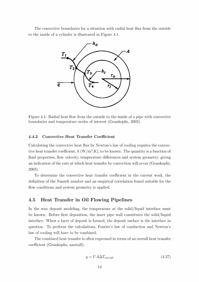
The convective boundaries for a situation with radial heat flux from the outside

to the inside of a cylinder is illustrated in Figure 4.1.

Figure 4.1: Radial heat flow from the outside to the inside of a pipe with convectiveboundaries and temperature nodes of interest (Geankoplis, 2003).

4.4.2 Convective Heat Transfer Coefficient

Calculating the convective heat flux by Newton’s law of cooling requires the convec-

tive heat transfer coefficient, h (W/m2.K), to be known. The quantity is a function of

fluid properties, flow velocity, temperature differences and system geometry, giving

an indication of the rate at which heat transfer by convection will occur (Geankoplis,

2003).

To determine the convective heat transfer coefficient in the current work, the

definition of the Nusselt number and an empirical correlation found suitable for the

flow conditions and system geometry is applied.

4.5 Heat Transfer in Oil Flowing Pipelines

In the wax deposit modeling, the temperature at the solid/liquid interface must

be known. Before first deposition, the inner pipe wall constitutes the solid/liquid

interface. When a layer of deposit is formed, the deposit surface is the interface in

question. To perform the calculations, Fourier’s law of conduction and Newton’s

law of cooling will have to be combined.

The combined heat transfer is often expressed in terms of an overall heat transfer

coefficient (Geankoplis, aarstall):

q = UA∆Toverall (4.27)

14

where q (W) is the rate of heat transfer, U (W/m2.K) is the overall heat transfer

coefficient, A (m2) is the interface area at which heat transfer occurs and ∆Toverall

(K) is the temperature difference between the average bulk flow temperature and

the ambient temperature.

For radial heat flux a cylinder [. . . ], Equation (4.6) and Equation (4.26) can be

combined to:

q = hiAwi(T1 − T2) =T2 − T3

(r2 − r1)/(kAAlm,A)= hoAwo(T3 − T4) (4.28)

where hi (W/m2.K) is the inner convective heat transfer coefficient, Ai (m2) is

the inner pipe wall (solid/liquid interface area), T1 (K) is the average bulk flow

temperature, T2 (K) and T3 (K) are the temperatures at the inner and outer pipe

wall, respectively, r2 (m) is the outer pipe radius, r1 (m) is the inner pipe radius,

kA (W/m.K) is the conductive heat transfer coefficient of the pipe, Alm,A (m2) is

the log mean area of the pipe, ho (w/m2K) is the outer heat transfer coefficient, Ao

(m2) is the outer pipe wall area and T4 (K) is the ambient temperature.

For an oil flowing pipeline with an existing layer of deposit, Equation (4.28) can

be written as:

q = hiAdep(Tb − Tdep) =Tdep − Twi

(rwi − rdep)/(kdepAlm,dep)

=Twi − Two

(rwo − rwi)/(kpipeAlm,pipe)=hoAwo(Two − Tsea)

(4.29)

where hi (W/m2.K) is the inner convective heat transfer coefficient, Adep (m2) is the

surface area of the deposit, Tb (K) is the average bulk flow temperature, Tdep (K) is

the temperature at the oil/deposit interface, Twi (K) is the temperature at the inner

pipe wall, rwi (m) is the inner pipe radius, rdep (m) is the effective flow radius, kdep

(W/m.K) is the thermal conductivity of the deposit, Alm,dep (m2) is the log mean

area of the deposit, kpipe (W/m.K) is the thermal conductivity of the pipe, Two (K)

is the temperature at the outer pipe wall, ho (W/m2K) is the outer convective heat

transfer coefficient, Awo (m2) is the outer pipe wall area, Two (m) is the temperature

at the outer pipe wall and Tsea is the ambient sea temperature.

The log mean areas of the deposit and the pipe are found by Equation (4.10)

and Equation (4.11), respectively. If there is no deposit in the pipe line, the second

term in Equation (4.29) falls out.

15

5 Mass Transfer

Mass transfer is defined as mass in transit as the result of a species concentration

difference in a mixture (Incropera et al., 2011). Just as a temperature difference in

a media inevitably results in heat transfer, a difference in concentration of chemical

species in a mixture leads to transfer of mass. The current chapter presents the

theoretical foundation necessary for the understanding of the wax deposition process.

5.1 Diffusion

Mass transfer due to random molecular motion is known as diffusion. Diffusion

of mass is analogue to the situation with heat transfer by conduction, but unlike

conduction heat transfer, diffusion of a species always involves the movement of

molecules or atoms from one region to another.


The rate of mass diffusion, or mass flux, in a binary mixture of chemical species A

and B is given by Fick’s law (Incropera et al., 2011):

J ′′ = −DABdC

dr(5.1)

where J′′ (kg/s.m2) is the mass flux or amount of solute A in solvent B transferred by

diffusion per unit time and per unit area perpendicular to the direction of transfer,

DAB (m2/s) is a binary diffusion coefficient, also known as the mass diffusivity, anddCdr

(kg/m4) is the radial concentration gradient. The minus sign in the equation

reflects that mass diffusion occurs in the direction of decreasing concentration.

The diffusion coefficient, DAB (m2/s), provides an indication of the rate at which

species A is transferred through species B by the diffusion process. The binary

diffusion coefficient is analogue to the kinematic viscosity in momentum transfer

and the thermal conductivity coefficient in heat transfer, that is, they represents

the proportionality constant, δ, in Equation (3.1). A correlation for calculation of

the diffusion coefficient for calculation of wax transfer in oil, Dwo (m2/s) will be

presented in Appendix C.

5.2 Dimensionless Numbers in Mass Transfer

The dimensionless numbers applied in the mass transfer calculations, are the Schmidt

number (Sc) and the Sherwood number (Sh).

16

5.2.1 Schmidt Number

The Schmidt number equals is defined as the ratio of kinematic viscosity to mass

diffusivity and provides a measure of the relative effectiveness of mass transport by

diffusion (Incropera et al., 2011):

Sc =ν

DAB

(5.2)

where ν (m2/s) is the kinematic viscosity and DAB (m2/s) is the binary diffusion

coefficient. The Schmidt number will be used in the calculations of the turbulent

mass diffusivities as presented below.

5.2.2 Sherwood Number

The Sherwood number equals a dimensionless concentration gradient at the surface

of a body. It provides a measure of the convection mass transfer occurring at the

surface and is defined as (Incropera et al., 2011):

Sh =kMd

Dwo

(5.3)

where kM (m/s) is the mass transfer coefficient, d (m) is the inner pipe diameter

and DAB (m2/s) is the binary diffusion coefficient. The Sherwood number will be

used to determine the mass transfer coefficient in the numerical modeling.

5.3 Fick’s Law in the Turbulent Flow Regime

Fick’s law, as defined by Equation (5.1), is only valid in the laminar flow regime.

Semi-empirical correlations can again be applied to extend the area of validity to the

turbulent flow regime. With the contribution from turbulent flow included, Fick’s

law is written as (Geankoplis, 2003):

J ′′ = −(DAB + εm)dC

dr(5.4)

where DAB (m2/s) is the binary diffusion coefficient, εm (m2/s) is the turbulent mass

diffusivity and dCdr

(kg/m4) is the concentration gradient in the mixture.

The turbulent, or eddy, mass diffusivity is defined by Prandtl mixing length

theory (Geankoplis, 2003):

εmDAB

=Sc

ScT

ε

ν(5.5)

where εm (m2/s) is the turbulent mass diffusivity, DAB (m2/s) is the binary diffusion

coefficient, Sc is the Schmidt number, ScT is the turbulent analogy to the Schmidt

17

number, ε (m2/s) is the eddy diffusivity and ν (m2/s) is the kinematic viscosity.

The turbulent analogy to the Schmidt number expresses the ratio of turbulent

mass diffusivity to molecular mass diffusivity:

ScT =ε

εm(5.6)

where ε (m2/s) is the momentum diffusivity and εm (m2/s) the turbulent mass

diffusivity. The momentum diffusivity is given by Equation (4.24).

18

6 Paraffin Wax

Crude oil is a mixture of a range of hydrocarbons including paraffins, aromatics,

naphtens, resins and asphaltens (Venkatesan, 2004). One of the problems associated

with hydrocarbon production, is the precipitation of paraffin molecules when the oil

is cooled leading to deposition. The current chapter introduces the chemistry and

physics behind wax deposition and presents methods to deal with the challenge in

the field.

6.1 Chemistry of Wax

Paraffin wax is a reference to linear chain alkanes (n-paraffins) containing more than

16 carbon atoms (Leontaritis et al., 2003). The general chemical formula of paraffins

is CnH2n+2. Depending on the chemical composition, paraffins might be in either

a gaseous, liquid or solid phase under ambient conditions. Paraffins with less than

four carbon atoms (C1-C4) will be at a gaseous state, paraffins with five to sixteen

carbon atoms (C5-C16) at a liquid state, and the series of C16-C70+, causing the

encountered wax deposition problems, will be in a solid state (Leontaritis et al.,

2003).

The carbon number distribution of paraffins in crude oils varies from one fluid

to another. Most of the paraffins found in crudes are in the range from C18-C65

(Ekweribe et al., 2008). To determine the exact wax composition, a laboratory

analysis will have to be conducted for each fluid in question. One method widely

used is the High Temperature Gas Chromatography (HTGC). The molecular weight

distribution of the hydrocarbons is then characterized as a function of the carbon

number, that is, the weight percent of all hydrocarbons with a certain carbon number

is identified (Singh et al., 2011).

6.2 Wax Appearance

Wax separation in hydrocarbon containing systems is mainly driven by thermo-

dynamic interaction. Because waxy crystals are incompressible and liquid hydro-

carbons only slightly compressible, a change in pressure induces little or no wax

appearance. Thus, a pressure drop at dynamic or static conditions has almost no

effect on wax precipitation. The separation of the heaviest components, is rather a

result of heat loss (cooling) from the liquid to the surroundings (Leonaritis et al.,

2003; Villazon and Civan, 2009).

The wax appearance temperature, is defined at the point where 0.02 mole percent

of the wax particles has precipitated out of solution, creating a binary mixture of

oil and wax (Singh et al., 2011). Since the solubility of wax is decreasing with

19

decreasing temperature, a lower cloud point will result in a later occurrence of wax

in solution, favorable for the situation.

The location of the WAT separates one region containing oil in a liquid phase

and waxy crystals in a solid phase, and another region in which the wax has not

precipitated out of solution yet (Villazon and Civan, 2009). The wax appearance

boundary where the flow is single phase above it and multiphase below, is in other

words inferred from the temperature profile.

There are several existing methods to determine the WAT, among those the

Cross Polar Microscopy (CPM) and the Differential Scanning Calorimetry (DSC).

Modeling of wax precipitation and subsequent deposition is found to be highly sen-

sitive towards the WAT prediction ability (Villazon and Civan, 2009). Because of

the importance of the parameter, it is recommended to make use of two indepen-

dent techniques to obtain a sufficient degree of accuracy when determining the WAT

(Venkatesan and Fogler, 2004; Venkatesan and Creek, 2010).

6.3 Deposit Formation

When oil in the near-wall region is cooled below the WAT, it starts to gel at the

pipeline wall. The deposition, or gelation, is a result of flocculation of orthorhombic

wax crystallites appearing in the fluid during cooling; the precipitated wax crystals

are forming a network. The gel deposited does not consist of pure solidified paraffins,

but is rather a wax-oil mixture containing a large fraction of oil trapped in a 3-D

network of wax crystals (Singh et al., 2000).

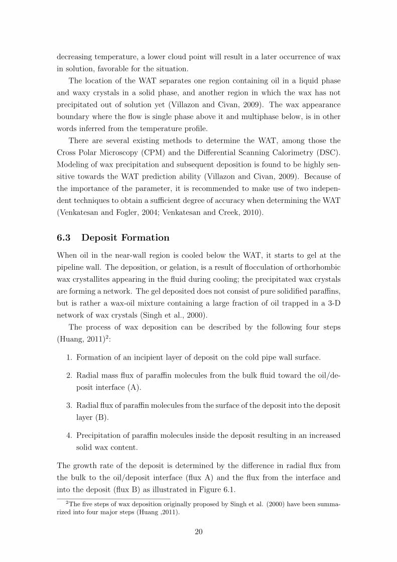
The process of wax deposition can be described by the following four steps

(Huang, 2011)2:

1. Formation of an incipient layer of deposit on the cold pipe wall surface.

2. Radial mass flux of paraffin molecules from the bulk fluid toward the oil/de-

posit interface (A).

3. Radial flux of paraffin molecules from the surface of the deposit into the deposit

layer (B).

4. Precipitation of paraffin molecules inside the deposit resulting in an increased

solid wax content.

The growth rate of the deposit is determined by the difference in radial flux from

the bulk to the oil/deposit interface (flux A) and the flux from the interface and

into the deposit (flux B) as illustrated in Figure 6.1.

2The five steps of wax deposition originally proposed by Singh et al. (2000) have been summa-rized into four major steps (Huang ,2011).

20

Figure 6.1: An illustration of the principles of wax deposition by molecular diffusion.The stippled line represents the centerline of the pipe and the thicker line the pipewall (Huang, 2011).

The driving force for deposition is the radial concentration gradient causing a

mass flux of wax molecules towards the inner pipe wall (Venkatesan, 2004). As the

concentration gradient is inferred from the temperature gradient, the temperature

profile in the pipeline is required when performing wax deposit simulations. The

radial concentration gradient is referred to as the mass driving force for wax deposi-

tion and the temperature radial gradient, ordifference, is referred to as the thermal

driving force (Huang, 2011).

6.4 Wax Handling

To avoid wax crystallization or to remove already existing deposits, various tools of

chemical and mechanical nature can be applied. To inhibit the formation of deposit

or to modify the WAT, paraffin inhibitors or dispersants can be used, preventing

agglomeration and deposition. For remediation of deposits already formed, the use

of hot solvents is a possible solution.

Examples of mechanical methods applied, are pipeline electrical heating and

pigging (mechanical scrapping), the latter being one of the most frequently used

remediation techniques in the field (Benall et al., 2008; Lee, 2008; Huang, 2011;

Singh et al., 2011). Paraffin wax deposition can also be prevented by insulation

of the pipelines, either by using external insulating coating or pipe-in-pipe systems

(Leontartis et al., 2003; Schulkes, 2013; Stokkenes, 2013).

21

7 Literature

The literature study introduces the possible mechanisms behind paraffin wax deposi-

tion and presents the theoretical foundation of the analytical and numerical models,

important for understanding of the presented results from the simulations in later

chapters.

7.1 Wax Deposition Mechanisms

Calculation of the radial mass transport of wax molecules in the viscous sub-layer

is considered one of the most important factors in the prediction of wax deposition

(Lee, 2008). A comprehensive study of the mechanisms responsible for wax depo-

sition was conducted by Burger et al. (1981), a work that has been a widely cited

reference since. Burger et al. (1981) identified four possible mechanisms responsible

for wax deposition: Molecular diffusion, Brownian diffusion, shear dispersion and

gravitational settling (Burger et al., 1981).

In the early 2000s, Azevedo and Teixeira (2003) did a review of the modeling

of wax deposition mechanisms. Molecular diffusion of paraffins, as described by

Burger et al. (1981), was acknowledged as the dominant mechanism responsible for

paraffin wax deposition. It was argued that experimental evidence suggests that

gravity settling and shear dispersion do not contribute significantly in the process.

However, not enough experimental evidence was found to exclude the possibility of

Brownian diffusion taking part (Azevedo and Teixeira, 2003).

A paper of more recent date states that the overall consensus in the field is

that molecular diffusion in the viscous sub-layer is the dominant mechanism of wax

deposition (Singh et al., 2011). Rønningsen (2012) is somewhat more careful in his

formulation, using the term fairly well-established when commenting upon molecular

diffusion as an important factor in control of the amount of wax molecules available

for deposition in the pipeline.

7.2 Wax Deposition Modeling

A number of mathematical models have been developed for the purpose of wax

deposit prediction. Among those are the models presented, representing two different

approaches towards wax deposit modeling in terms of mathematics and fundamental

assumptions.

22

7.2.1 Analytical Model

In the analytical model, the mass rate of wax transfer is calculated by Fick’s law.

The radial flux of wax molecules is computed with the assumption of thermodynamic

equilibrium in the mass transfer boundary layer, that is, the wax concentration is, in

other words, assumed to follow the solubility at every point in the pipeline (Azevedo

and Teixeira, 2003; Lee, 2008; Aiyejina et al., 2011).

The assumption of thermodynamic equilibrium in the viscous sub-layer is found

to be valid in the laminar flow regime only. Under turbulent flow conditions, as

encountered in oil flowing pipelines, the concentration field is found to be correlated

to the temperature field and must, in order to obtain correct modeling, be taken

into consideration (Venkatesan and Fogler, 2004).

When the difference in solubility and actual wax concentration in the boundary

layer is significant, the analytical model is expected to result in an over prediction of

wax deposits. The situation situation arises in turbulent flow, when the precipitation

kinetics of wax molecules in the boundary layer is slow (Venkatesan and Fogler, 2004;

Lee, 2008; Huang, 2011).

The analytical model assumes a constant weight fraction of wax in deposit during

the deposition process. This is a simplification of the situation, as the process

of deposition is described by a radial flux of wax molecules from the bulk to the

oil/deposit interface followed by a flux of molecules from the interface and into the

deposit where further precipitation of paraffin wax occurs (Singh et al., 2000). An

interesting study, however outside the scope of the current work, is an evaluation of

the growing wax content in the deposit and its consequences for deposit thickness

prediction and selection of remediation techniques.

7.2.2 Numerical Model

The implemented numerical model has been stepwise developed from a general math-

ematical model describing the process of wax deposition (Singh et al., 2001). Based

on the balance of energy and mass, a set of equations to calculate the growth rate

and aging of wax deposits was derived. To calculate the mass flux of wax molecules,

the convective mass transfer coefficient obtained from the laminar Sherwood number

was applied.

The model was found to successfully predict the results of wax deposition under

laminar flow conditions, but to over estimate the deposit thickness in the turbulent

flow regime (Lee, 2008). The over prediction is explained by a neglect of precipitation

of wax molecules in the oil phase, physically correct under laminar flow conditions,

but an important feature in the turbulent flow regime where the rate of cooling is

relatively slow (Huang, 2011).

23

A refinement of the model was presented by Venkatesan and Fogler (2004). The

basic equations derived by Singh et al. (2001) was applied to calculate the growth

rate of the deposit, but with the convective mass transfer rate estimated by the

Sherwood number and an experimentally obtained solubility curve (Lee, 2008). The

model showed to under predict the deposit thickness, a finding believed to be a result

of supersaturated wax molecules in solution without sufficient time to precipitate

that was not accounted for (Huang, 2011).

Based on the same equations, Lee (2008) developed a wax deposition model

applicable in both the laminar and the turbulent flow regime. The finite difference

method (FDM) was applied on a coupled set of heat and mass transfer equations and

a precipitation rate constant was included to account for precipitation kinetics of

the wax molecules. The correct results was explained by the impact of precipitation

kinetics on the diffusion mass flux in the boundary layer, reducing the diffusive

mass transfer rate of wax molecules significantly (Lee, 2008). The model has been

acknowledge as a correct correlation of the phenomena of heat and mass transfer

that provides a robust and rigorous way of predicting wax deposition in both flow

regimes (Aiyejina et al., 2011).

24

8 Effective Thermal Conductivity of Two Com-

ponent Systems

Correct wax deposition modeling requires correct modeling of the effective ther-

mal conductivity of the wax deposit. Since the gel layer at the pipeline wall is a

two component system composed of paraffin wax and oil, computational models to

determine the effective thermal conductivity of a heterogenous material has been

investigated

8.1 Thermal Conductivity

The effective thermal conductivity of heterogeneous materials is strongly affected

by its composition and structure. Several methods to determine the property exists.

Some includes the use of empirical parameters to account for variations in com-

position and structure, others make use of numerical techniques (Bunthebart and

Jobman, 2008).

In many applications analytical models are preferred. The main advantage of

an analytical model is the rapid and low cost calculations, and the independency

of empirical correlations. Each of the analytical models presented have a physi-

cal basis and are producing results of reasonable accuracy, even with an unknown

microstructure (Wang et al., 2006; Bunthebart and Jobman, 2008).

In the current work, the thermal conductivity of oil, wax, pipe and deposit are

required. The thermal conductivity of oil, wax and pipe duplex steel, being the

material of the pipe, are table values reported in Table 4. The effective thermal

conductivity of the wax deposit will have to be calculated from one of the proposed

models as it is a binary mixture of oil and wax.

Table 4: Thermal conductivity values of oil, paraffin wax and duplex steel to beapplied in the wax deposit models (Gudmundsson, 2012; Mirazizi, 2012).

SubstanceThermal Conductivity

[W/m.K]

Oil 0.10

Paraffin Wax 0.25

Duplex Steel 20

25

8.2 Stratified Models

The simplest analytical models are the Parallel model and the Series model. With

the heat flow being in the vertical direction, the Parallel model assumes a distribu-

tion of the two components in distinct vertical layers. Mathematically, the model is

expressed as (Wang et al., 2006):

ke = v1k1 + v2k2 (8.1)

where ke (W/m.K) is the effective thermal conductivity of the material, k1 (W/m.K)

is the thermal conductivity of the first component, k2 (W/m.K) is the thermal

conductivity of the second component, and v1 and v2 are the volume fractions of

the two components.

The Series model assumes a distribution of the two components in distinct hor-

izontal layers, the heat flow still being in the vertical direction. The model is given

as (Wang et al., 2006):

ke =

(v1

k1

+v2

k2

)−1

(8.2)

with the thermal conductivities and volume fractions as declared above.

The volume fractions can further be expressed as (Awad and Muzychka, 2008):

v2 = (1− v1) (8.3)

where v1 is the volume fraction of the first component and v2 is the volume fraction

of the second component.

8.3 Maxwell-Eucken Model

A conductivity formula suitable for two component systems consisting of a continu-

ous and a dispersed phase was presented by Maxwell (1904) and further developed

by Eucken (1940), resulting in the Maxwell-Eucken Model (Serpil and Servet, 2006).

The model assumes the dispersion of small spheres of one substance within a con-

tinuous matrix of a different component. Based on the thermal conductivity of the

components, two variations of the model exists.

8.3.1 Maxwell-Eucken 1

If the thermal conductivity of the continuous phase is higher than the thermal

conductivity of the dispersed phase (kcont > kdisp), the Maxwell-Eucken 1 (ME1) is

applicable (Awad and Muzychka, 2008):

26

k1 > k2

ke =k1v1 + k2v2

3k1

2k1+k2

v1 + v22k1

2k1+k2

(8.4)

where ke (W/m.K) is the effective thermal conductivity of the material, k1 and k2

(W/m.K) are the thermal conductivity of the two components and v1 and v2 are

the two volume fractions.

8.3.2 Maxwell-Eucken 2

In the reversed cases, if the thermal conductivity of the continuos phase is less than

the thermal conductivity of the dispersed phase, (kcont < kdisp), the Maxwell-Eucken

2 (ME2) is suitable (Awad and Muzychka, 2008):

k1 < k2

ke =k2v2 + k1v1

3k2

2k2+k1

v2 + v12k2

2k2+k1

(8.5)

with the thermal conductivities and volume fractions as above.

8.4 Effective Medium Theory

The basic assumption of the Effective Medium Theory (EMT), is a total random

distribution of the two components within a material (Wang et al., 2006). The

model is well suited in situations where neither of the components are continuous

or dispersed, but rather randomly distributed (Awad and Muzychka, 2008).

v1k1 − kek1 + 2ke

+ v2k2 − kek2 + 2ke

= 0 (8.6)

where the variables are as before.

Rearranging Equation (8.6), a quadratic equation suitable for implementation in

the computer program is obtained:

2(v1 + v2)k2e − (2v1v2 − v1k2 − v2k2 + 2v2k2)ke − (v1 + v2)k1k2 = 0 (8.7)

ke =−b ±

√b2 − 4ac

2a(8.8)

27

where

a = 2(v1 + v2)

b = −(2v1v2 − v1k2 − v2k2 + 2v2k2)

c = −(v1 + v2)k1k2

If Equation (8.8) yields two results, the positive outcome (ke > 0) is the value of

the effective thermal conductivity to be used.

8.5 Evaluation of Model Applicability

The applicability of the five effective thermal conductivity models for the wax deposit

have been evaluated on the basis of structure. The layer of deposit is made up of

a large fraction of oil trapped in a 3-D network of wax crystals, hence, the criteria

for using the Parallel and the Series models are not met, as those requires stratified

deposition into distinct layers.

The conclusion is confirmed by the microscope observations of a typical wax-

oil gel in Figure 8.1. The image reveals that the wax-oil gel does not deposit into

stratified layers. Additionally, neither the oil (black) nor the wax crystals (white)

appear as small spheres within a continuous matrix of the other component. Hence,

the Maxwell-Eucken Models are ruled out for application in the current work.

Figure 8.1: Microscope observations of a wax-oil gel (polarized light microscopyimage). The oil is dark and the wax crystals are the bright (Venkatesan, 2004).

28

Instead, the averaging scheme of the Effective Medium Theory seems to be a

reasonable model in the case of determining the effective thermal conductivity of

the wax deposit with the assumption of a random distribution of the components. As

a consequence, the EMT has been applied in the implemented wax deposit models.

A schematic representation of the model structures are summarized in Figure G.1

in Appendix G.

8.6 Application of Models

To quantify the deviation, of source of error, that would arise if one of the former

models were applied, the methods have been plotted as a function of wax. With

the EMT as a base case, the deviation in percentage is found to range between

-5.3% (Parallel model) and 11.1% (Series model). The graphs for the five effective

thermal conductivity models are given in Figure 8.2 and the numerical values of the

maximum deviation in Table 5.

Figure 8.2: The five effective thermal conductivity models of two component systemsplotted against weight fraction of wax in deposit. The EMT is found applicable forthe wax deposit modeling.

29

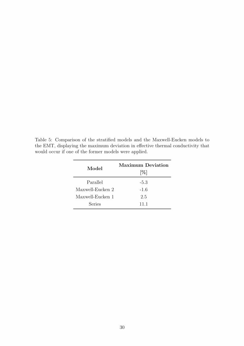
Table 5: Comparison of the stratified models and the Maxwell-Eucken models tothe EMT, displaying the maximum deviation in effective thermal conductivity thatwould occur if one of the former models were applied.

ModelMaximum Deviation

[%]

Parallel -5.3

Maxwell-Eucken 2 -1.6

Maxwell-Eucken 1 2.5

Series 11.1

30

9 Interface Temperatures

To establish the radial concentration gradient in the pipeline, being the mass driving

force for deposition, the temperature conditions in the system must be known. In

the current chapter, the influence of a layer of deposit on the thermal conditions

in the pipeline is examined. The aim is to see how the temperature at the deposit

surface changes with a layer of deposit and to evaluate if dynamic modeling of the

wax deposit process will be necessary or not.

9.1 Thermal Resistance for Conduction and Convection

Resistance is defined as the ratio of a driving potential to the corresponding transfer

rate. In case of thermal resistance, it is a measure of a substance’s resistance towards

heat flow (Incorpera and DeWitt, aarstall).

The thermal resistance for conduction heat transfer and convection heat transfer

are given by different expressions. For conduction, the thermal resistance is derived

from Fourier’s law and, in radial coordinates, given as (Geankoplis, 2003):

Rcond ≡Ts − T∞

q=r2 − r1

kAlm(9.1)

where Rcond (m2K/W) is the thermal resistance for conduction, Ts (K) is the tem-

perature of the surface, T∞ (K) is the temperature of the fluid, q (W) is the heat

transfer rate, r1 (m) is the inner radius of the cylinder, r2 (m) is the outer radius of

the cylinder, k (W/m.K) is the thermal conductivity of the cylinder and Alm is the

log mean area of the cylinder.

From Newton’s law of cooling, the thermal resistance for convection may be

derived (Incropera et al., 2011):

Rconv ≡Ts − T∞

q=

1

hA(9.2)

where Ts (K) is the temperature of the surface, T∞ (K) is the temperature of the

fluid, q (W) is the heat transfer rate, h (W/m2.K) is the convective heat-transfer

coefficient and A (m) is the area between surface and fluid.

Since the thermal resistances in a cylinder are in series (radial direction), a

total heat resistance can be expressed as the sum of the individual heat resistances


Rtot = Rin +m∑i=1

Rcond,i +Rout+ =n∑i=1

Ri (9.3)

where Rtot (m2K/W) is the total heat resistance, Rin (m2K/W) is the inner convec-

31

tive heat resistance, Rcond,i (m2K/W) is the individual conductive heat resistances,

Rout (m2K/W) is the outer resistance, and∑

Ri (m2K/W) is the sum of the indi-

vidual heat resistances. The index m is the total number of layers, and the index n

the number of layers plus the convective heat resistances (n = m+2).

9.2 Situation in the Oil Pipeline

In an oil flowing pipeline, the conductive thermal resistance of the pipe is found as:

Rpipe =1

(kpipeAlm, pipe)/(rwi − rwo)(9.4)

where Rpipe (m2K/W) is the heat resistances of the pipe, kpipe (W/m.K) is the

thermal conductivity of the pipe, Alm,pipe (m2) is the logarithmic mean area of the

pipe, rwi (m) is the inner wall radius and rwo (m) is the outer wall radius. The

conductive thermal resistance of a possible layer of wax deposit is given as:

Rdep =1

(kdepAlm, dep)/(rdep − rwi)(9.5)

where Rdep (m2K/W) is the individual heat resistance of the deposit, kdep (W/m.K)

is the thermal conductivity of the deposit, Alm,dep (m2) is the logarithmic mean

area, rdep (m) is the effective flow radius measured from the central line of the

interface pipe to the deposit interface and rwi (m) is the inner wall radius. The

logarithmic mean areas, Alm (m2) are calculated by Equation (4.11) and Equation

(4.10), respectively.

The inner convective heat resistance is calculated as:

Rin =1

hiAin(9.6)

where Rin (m2K/W) is the inner heat resistance, hi (W/m2K) is the inner heat

transfer coefficient, Ain (m2) is the interface area between oil and clean pipe wall if

no deposit is present or between oil and wax deposit if deposition has occurred.

The outer convective heat resistance is found as:

Rout =1

hoAwo(9.7)

where Rout (m2K/W) is the outer heat resistance, ho (W/m2K) is the outer heat

transfer coefficients and Awo (m2) is the outer pipe wall area or the interface area

between pipe and the surrounding sea water.

Expressing the heat flow in the system in terms of resistances, Equation (4.29)

is written as (Geankoplis, 2003):

32

q =Tb − Tsea

1/(hiAdep) + (rwi − rdep)/(kdepAlm,dep) + (rwo − rwi)/(kpipeAlm,pipe) + 1/hoAwo

q =Tb − Tsea

Ri +Rdep +Rpipe +Ro

=Tb − Tsea∑

R(9.8)

The contribution from the individual heat resistance to the total heat resistance

is, in percentage, found as:

contribution to heat resistance =R′

Rtot

· 100% (9.9)

where R′ (m2K/W) is the individual thermal resistance of interest and Rtot (m2K/W)

is the total thermal resistance.

9.3 Temperature Calculations

From Equation (4.28), expressing the radial heat flow in the system, the equations

to calculate the temperature at the wax deposit surface, the inner pipe wall and

the outer pipe wall can be derived. The temperature at the oil/deposit interface is

found as

Tdep = Tsub + qRi (9.10)

where Tdep (K) is the temperature at the oil/deposit interface, Tsub (K) is the

temperature in the near-wall region, q (W) is the radial heat flow and Ri (m2K/W)

is the inner heat resistance. If there is no wax deposit at the point of interest (clean

pipe wall), the temperature at the inner pipe wall is given as:

Twi = Tsub + qRi (9.11)

where Tdep (K) is the temperature at the oil/deposit interface, Tsub (K) is the

temperature in the near-wall region, q (W) is the radial heat flow and Ri (m2K/W)

is the inner heat resistance. If a layer of deposit exists, the inner wall temperature

is calculated as

Twi = Tdep + qRdep (9.12)

Twi (K) is the inner wall temperature, q (W) is the radial heat flow and Rdep

(m2K/W) is the individual heat resistance from the layer of deposit.

33

The outer wall temperature is in either case calculated as:

Two = Twi + qRpipe (9.13)

Two (K) is the outer pipe wall temperature and Rpipe (m2K/W) is the resistance of

the pipe.

9.4 Influence of the Wax Deposit

To examine the influence of the wax deposit on the thermal conditions in the pipeline,

the thickness of the deposit and the wax content have been evaluated separately.

First, the deposit thickness has been varied with the assumption of a constant wax

content in the deposit, then the deposit thickness has been kept constant and the

wax content has been varied.

9.4.1 Influence of Deposit Thickness

When investigating the influence of the deposit thickness on the thermal situation

in the pipeline, a deposit thickness ranging from 0-20 mm has been applied. This

covers the situation from a clean pipe wall to, what is characterized as, a severe wax

deposit buildup (Rønningsen, 2012).

Based on experiences from the Norwegian Continental Shelf, a wax fraction of

40 % in deposit has been applied (Rønningsen, 2012)3. The temperature in the

near-wall region at the point of interest is set equal to 25 ◦C and the ambient sea

temperature is assumed to hold 5◦C (Rønningsen, 1992).

9.4.1.1 Results The wax deposit is found to add a layer of insulation to the

system. With an increasing deposit thickness, the dominating heat resistance of

the system changes from being the outer convective heat resistance (-72.92%) to

the conductive heat resistance of the deposit (+75.54%). There is only a slight

reduction in the contribution of the inner heat resistance and the contribution of

the pipe as the deposit layer increases (-1.67% and -0.94%, respectively). The results

are presented in Table 6.

As a consequence of the increasing thermal insulation, the temperature at the

oil/deposit interface is found to increase as the layer of deposit grows. The tem-

peratures at the inner and outer wall are simultaneously decreasing. The numerical

values for the temperature changes of the simulated situation are given in Table

3The assumption of Rønningsen (2012) is based on experiences from the Norwegian ContinentalShelf where knowledge about wax content has been acquired from samples of wax from back flowof a stuck foam pig in the pipeline between the Heimdal and Brae A platforms in the North Sea.

34

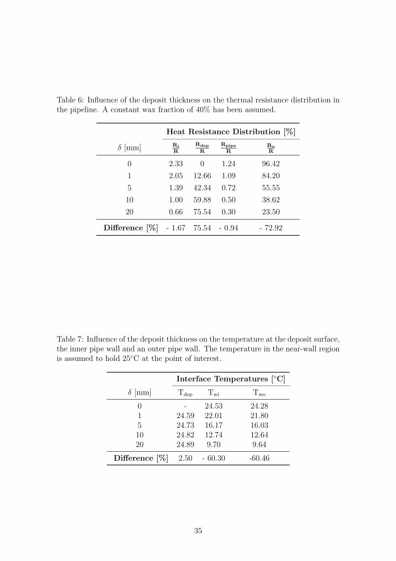
Table 6: Influence of the deposit thickness on the thermal resistance distribution inthe pipeline. A constant wax fraction of 40% has been assumed.

Heat Resistance Distribution [%]

δ [mm] Ri

R

Rdep

R

Rpipe

RRo

R

0 2.33 0 1.24 96.42

1 2.05 12.66 1.09 84.20

5 1.39 42.34 0.72 55.55

10 1.00 59.88 0.50 38.62

20 0.66 75.54 0.30 23.50

Difference [%] - 1.67 75.54 - 0.94 - 72.92

Table 7: Influence of the deposit thickness on the temperature at the deposit surface,the inner pipe wall and an outer pipe wall. The temperature in the near-wall regionis assumed to hold 25◦C at the point of interest.

Interface Temperatures [◦C]

δ [mm] Tdep Twi Two

0 - 24.53 24.281 24.59 22.01 21.805 24.73 16.17 16.0310 24.82 12.74 12.6420 24.89 9.70 9.64

Difference [%] 2.50 - 60.30 -60.46

35

7, shown an increase of 2.5% at the deposit surface and a decrease of -60.30% and

-60.46% at the inner and outer pipe walls, respectively.

9.4.2 Influence of Wax Fraction

Examining the influence of the weight fraction of wax in deposit, the thickness of

the layer has been kept constant at 20 mm. The investigated wax content ranges

from 5-70%, being data reported from the field (Venkatesan, 2004; Lee, 2008). The

temperature in the near-wall region at the point investigated is 25◦C and the ambient

temperature 5◦C.

9.4.2.1 Results A layer of deposit with a higher wax content is found to create

less resistance towards thermal flow than a layer of a corresponding thickness and

a lower wax content. The contribution from the inner heat resistance and the resis-

tance of the pipe are found to increase with 0.30% and 0.14%, respectively, whilst

the contribution of the deposit layer is reduced with -11.29% and the outer resistance

increased with 10.85% under the applied conditions when the wax content increases

from 5 to 70 %. The numerical results for varying wax contents are given in Table

8, showing what is commented upon.

Table 8: Influence of the weight fraction of wax in deposit on the thermal resistancedistribution in the pipeline. A deposit thickness of 20 mm has been applied.

Heat Resistance Distribution [%]

Wax [%] Ri

R

Rdep

R

Rpipe

RRo

R

5 0.50 81.39 0.23 17.8820 0.56 79.00 0.26 20.1740 0.60 75.54 0.30 23.5050 0.70 73.74 0.33 25.2370 0.80 70.10 0.37 28.73

Difference [%] 0.30 -11.29 0.14 10.85

The temperature at the oil/deposit interface is lower with a high content of wax

in the deposit, a finding caused by the thermal conductivity of wax being higher than

the thermal conductivity of oil. A deposit with a higher wax fraction will cause less

resistance towards heat flow than a layer of a corresponding thickness and a lower

wax content. At the inner and outer pipe wall, the temperatures will be higher with

a higher content of wax. The numerical values for the applied conditions are given

in Table 9.

36

Table 9: Influence of the weight fraction of wax in deposit on the temperature atthe deposit surface, the inner pipe wall and an outer pipe wall. The temperature inthe near-wall region is assumed to hold 25◦C at the point of interest.

Interface Temperatures [◦C]

Wax [%] Tdep Twi Two

5 24.91 8.62 8.5820 24.90 9.07 9.0240 24.89 9.70 9.6450 24.88 10.18 10.1270 24.86 10.86 10.78

Difference [%] -0.20 25.99 25.64

9.4.3 Discussion

With the assumption of a constant weight fraction of wax in the deposit, the insu-

lating effect of the layer has shown to increase with an increasing thickness. Varying

the wax content while keeping the deposit thickness constant, a higher wax fraction

is found to cause less resistance towards heat flow than a layer of corresponding

thickness with a lesser content of wax.

Assuming temperatures below the WAT and the existence of a radial tempera-

ture gradient in the pipeline, the deposit thickness and wax content are expected

to increase with time, acting as opposing mechanisms when it comes to thermal

resistance. Comparing the phenomena for the values of interest, the influence of the

deposit thickness is found to be greater than the influence of the wax content. The

percentage changes caused by an increased deposit thickness is given in the lower

row of Table 10 and the percentage changes caused by the increased wax content in

the last column, proving the deposit thickness to be the dominating factor.

The influence of the wax content in the deposit will not be further investigated in

the current thesis. It is noted that the wax content will affect the thermal conditions

in the pipeline, with a higher wax content causing the temperature at the deposit

surface to be slightly lower than is the case with a lower wax content. Hence, an

increased wax content in the deposit will cause a steeper thermal gradient, causing

less reduction in the thermal driving force for deposition than were the case without

aging. The consequences of an increasing wax content in the deposit is recommended

investigated as part of a future work.

Independent of the amount of wax in deposit, the temperature at the oil/deposit

interface will increase with a growing deposit thickness. The temperature at the

deposit surface will be brought closer to the average bulk flow temperature with

37

Table 10: Deposit surface temperature with a varying deposit thickness and weightfraction of wax in the deposit. In the lower row, the percentage change caused by theincreased deposit thickness is given, and in the column to the right the percentagechange caused by the increasing wax content.

Wax [%]

δ [mm] 5 20 40 50 70 Difference [%]

1 24.61 24.60 24.59 24.58 24.57 -0.165 24.77 24.75 24.73 24.72 24.70 -0.2810 24.85 24.84 24.82 24.80 24.78 - 0.2820 24.91 24.90 24.89 24.88 24.86 -0.20

Difference [%] 1.55 1.51 1.48 1.43 1.35

time, resulting in a lesser temperature gradient across the viscous sub-layer. A

lower temperature gradient means a reduced thermal driving force for deposition.

The result is a non-linear growth of the deposit thickness, where the mass rate of wax

transfer is expected to be fast initially and to slow down as the thickness of the layer

increases. To avoid over estimation of the final deposit thickness, the simulations

will have to be dynamic.

38

10 Analytical Modeling

In the analytical model, Fick’s law is applied to estimate the mass flux of wax

with the assumption of thermodynamic equilibrium in the viscous sub-layer. In the

current chapter, the mathematical model implemented in MATLAB is derived and

the results from simulations performed on the Norne crude oil under real field is

presented.

10.1 Application and Assumptions

The analytical wax deposition model is applicable for oil transporting pipelines.

The governing equations, and hence the model, is valid in situations where the

flow is non-reacting and there is no thermal energy generation in the fluid. The

fluid mixture is assumed to be incompressible and the density consequently treated

as constant. The density of wax is assumed equal to the density of oil, and the

fluid mixture is treated as a Newtonian fluid, that is, the viscosity is considered

independent of shear rate.

The maximum amount of wax dissolved in solution is determined by the wax

appearance temperature and the solubility function. Above the wax appearance

limit, the flow is single-phase (liquid only) and below it is a two phase mixture of

liquid oil and solid wax. Zero water content and zero gas rate in the system is

assumed.

The seawater surrounding the pipeline is assumed to hold a constant temperature

of 5 ◦C (Rønningsen et al., 1992). The fluid flow is treated as one dimensional,

with net flow of oil in the axial direction only, and the fluid velocity is assumed

constant. Molecular diffusion from the near-wall region to the solid/liquid interface

is considered as the sole mechanism for wax deposition, and the precipitated wax

molecules in the viscous sub-layer are expected to deposit at the solid/liquid interface

where the precipitation occurs. No shear-removal is included and there is no thermal

insulation of the system.

The Effective Medium Theory model has been applied for the calculation of the

effective thermal conductivity of the wax deposit, and the Dittus-Boelter correla-

tion is found applicable to calculate the inner convective heat transfer coefficient.

Thermodynamic equilibrium at every point in the pipeline has been assumed and

the weight fraction of wax in deposit is assumed.

10.2 Flow Regions

Turbulent flow in a cylinder can be divided into three flow regions. Adjacent to

the wall, there is a viscous sub-layer in which transfer processes are dominated by

39

diffusion. Next, there is a buffer layer, or transition zone, in which transfer by

diffusion and turbulent mixing are comparable. In the center of the pipe, the flow is

turbulent and the transport phenomena are dominated by turbulent mixing (White,

2008).

In operative oil flowing pipelines, turbulent diffusivities of temperature and chem-

ical species are assumed to cause an uniform distribution of temperature and con-

centration over the cross-sectional area of the pipe (Aijeijna et al., 2011). Since

the transport of wax is controlled by the prevailing gradients in the viscous sub-

layer, the thickness of the layer must be known to establish the temperature and

concentration profiles in the near-wall region (Azevedo and Teixeira, 2003).

To determine the extension of the flow regions, von Karman defined a dimen-

sionless wall distance (Kay and Nedderman, 1985):

y+ =y

yτ(10.1)

where y+ is the dimensionless wall distance, y (m) is the actual distance from the

pipe wall and yτ (m) is the friction distance found as:

yτ =µ

τwρ(10.2)

where µ (Pa.s) is the dynamic viscosity, ρ (kg/m3) is the fluid density and τw (Pa)

is the wall shear stress. The wall shear stress is given by (Incropera et al., 2011):

τw = µdu

dy=

1

2fρu2 (10.3)

where dudy

is the local velocity gradient, f is the friction factor, ρ (kg/m3) is the fluid

density and u (m/s) is the average flow velocity. The flow regions are divided into

(Kay and Nedderman, 1985):

y+ ≤ 5 Viscous sub-layer

5 < y+ < 30 Buffer layer

y+ ≥ 30 Turbulent core

10.3 Temperature Calculations

To establish the concentration gradient at the solid/liquid interface, the temperature

in the viscous sub-layer and at the solid/liquid interface must be known. To deter-

mine those quantities, the average bulk flow temperature throughout the pipeline is

required.

40

10.3.1 Average Bulk Flow Temperature

The average bulk flow temperature, or the lateral temperature profile, is calculated

as (Gudmundsson, 2009):

Tb = Tsea + (Ti − Tsea)exp(−UπdmCp

L

)(10.4)

where Tb (K) is the temperature of the bulk flow at the distance of interest, Tsea

(K) is the ambient temperature, Ti (K) is the inlet temperature, U (W/m2.K) is

the overall heat transfer coefficient, d (m) is the inner pipe diameter, m (kg/s) is

the mass flow rate, Cp (J/kg.K) is the heat capacity of oil and L (m) is the distance

of interest.

10.3.2 Boundary Layer Temperature

For a subsea pipeline cooled from the outside, the following equations can be used

to obtain the temperature profile (Kay and Nedderman, 1985):

T+ =

Tw

+ + (Pr)y+ y+ ≤ 5

Tw+ − 5Pr + 5ln[0.2(Pr)y+ + (1− Pr)] 5 < y+ < 30

Tw+ − 5Pr + 5ln[0.2(Pr)y+ + (1− Pr)]− 2.5lny

+

30y+ ≥ 30

(10.5)

where T+w is the dimensionless wall temperature, Pr is the Prandtl number andy+

is the dimensionless wall distance, given by:

y+ =ρu∗y

µ(10.6)

where ρ (kg/m3) is the density of the fluid, y (m) is the actual distance from the wall

and µ (Pa.s) is the dynamic viscosity and u∗ is the dimensionless friction velocityis,

given as:

u∗ =

√τwρ

= u

√f

8(10.7)

where τw (Pa) is the wall shear stress, u (m/s) is the average flow velocity and f is

the friction factor. The dimensionless wall temperature is then found as:

Tw+ = T

(ρCpu

∗

Q/A

)(10.8)

where T (◦C) is the temperature of interest, ρ (kg/m3) is the fluid density, Cp (J/K)

is the heat capacity of the fluid, u∗ is the friction velocity and the heat flow Q (W)

41

divided by the heat transfer area A (m2) equals the heat flux, q (W/m2). Finally,

the temperature in the viscous sublayer is then determined:

Tsub = T+ q

ρCpu∗(10.9)

where T+ is the dimensionless wall temperature, q (W/m2) is the radial heat flux,

ρ (kg/m3) is the fluid density, Cp (J/K) is the heat capacity of the fluid and u∗ is

the friction velocity.

10.3.3 Interface Temperatures

The temperatures at the inner pipe wall, the outer pipe wall and at the deposit

surface are calculated by Equation (9.10)-(9.13). When there is no deposit in the

pipeline, the inner wall represents the interface are at which deposition occurs and

the temperature of interest. When first deposition has occurred, the deposit surface

is the area at which wax deposits and the temperature at the oil/deposit interface

is the one sought for.

10.4 Wax Deposit Calculations

Based on the assumptions presented Fick’s law is applied to determine the mass

transfer rate in a binary mixture of wax and oil (Burger et al., 1981; Azevedo and

Teixeira, 2003; Sarica and Volk, 2004; Lee, 2008; Benall et al., 2008; Aiyejina, 2011;

Mirazizi et al., 2012) :

dm

dt= −ρwDwoAi

dC

dr

∣∣∣i

(10.10)

where dmdt

(kg/s) is the mass rate of wax transfer in oil, ρw (kg/m3) is the density of

solid wax, Dwo (m2/s) is the diffusion coefficient of wax in oil, Ai (m2) is the surface

area at which the deposition occurs, C (volume fraction) is the concentration of wax

in oil, and r (m) is the radial coordinate at the point of interest measured from the

centerline of the pipe. The radial concentration gradient, dCdr

is evaluated at the

solid/liquid interface.

Since the density of wax is assumed equal to the density of oil, the weight percent

of wax in solution corresponds to the volume percent of wax in solution. As a result,

the solubility functions in Appendix E can be used directly in the calculations.

The interface area available for deposition, Ai, can be calculated as:

Ai = 2πrL (10.11)

42

where r (m) is the radial coordinate of interest and L (m) is the length of the pipe.

If there is no wax deposit at the place of interest, the solid/liquid interface radius

equals the inner pipe radius, r(t) = ri. If deposition has occurred, the solid/liquid

interface equals the inner pipe radius minus the deposit thickness, r(t) = ri - δ(t).

The deposit thickness, δ (m), is found by integration of Equation (10.10):

δ(t) = −DwodC

dr

∣∣∣it (10.12)

where δ(t) (m) is the deposit thickness at the time of interest, Dwo (m2/s) is the

binary diffusion coefficient of wax in oil and dCdr

(unit) is the radial concentration

gradient at the solid/liquid interface.

As the driving force for deposition is found to change with time, the deposit

thickness will be calculated as:

δ(t+ ∆t) = δ(t) +

(−Dwo

dC

dr

∣∣∣i∆t

)(10.13)

where δ(t) (m) is the deposit thickness in the previous time step and ∆t (s) is the

time step.

10.5 Simulations

The conducted simulations are performed on the Norne crude oil with subsea pipelines

under realistic field condition. For determination of the viscous sub-layer thickness,

the outer limit (y+ = 5) has been applied. The outer limit is chosen to obtain the

maximum value of wax transfer across the sub-layer; as the temperature difference

over a thicker sub-layer is greater than over a thinner sub-layer, the driving force for

deposition will be at its maximum when the maximum sub-layer thickness is applied.

The resulting wax transfer represents an upper limit for wax deposition and, hence,

a worst case scenario to be applied in planning and design. In the analytical model,

a pipelenght of 10000 meter is chosen simulated, however no limitations regarding

pipe sizing exists. The remaining input values are found attached in Appendix F.

10.5.1 Results

The thickness of the wax deposit is found to increase with time. With the applied

conditions, the temperature in the viscous sub-layer reaches the WAT after 1284

meter. The maximum deposit thickness is observed at the point where the WAT

is reached, and from this point on the thickness of the deposit gradually decreases

throughout the pipeline.

The wax deposit profiles after one, two and seven days are plotted in Figure

10.1, graphically displaying the findings commented upon above. In Table 11, the

43

maximum deposit thicknesses (encountered at 1284 meter) and the thickness at the

outlet of the simulated pipeline are given.

Figure 10.1: Deposit thickness profiles after one day, two days and seven days ob-tained by the analytical model. The maximum deposit thickness is obtained at 1284meter, where the WAT is reached in the near-wall region.

The maximum deposit thickness is found to increase from 3.9 mm to 16.6 mm

from the first to the seventh day, hence, the growth rate of the deposit is found to

decrease with time. The findings are in correspondence with the results in Chapter

9, indicating a correct implementation of the model.

Table 11: Deposit thickness values obtained by the analytical model. The thicknessat 1284 meter is the maximum deposit thickness and the values at 10000 meter isat the end of the simulated pipeline.

Deposit Thickness [mm]

Time 1284 m 10000 m

1 day 3.9 0.72 days 6.9 1.37 days 16.6 4.1

44

The results of the analytical simulations will be compared to the numerical simula-

tions and results obtained by commercial software in Chapter 12.

45

11 Numerical Modeling

In the numerical model, the Finite Difference Method (FDM) is applied on a cou-

pled set of heat and mass equations. By including a precipitation rate constant,

the precipitation of wax molecules is accounted for and the correlation that exists

between heat and mass transfer in the turbulent flow regime is accounted for.

11.1 Application and Assumptions

The numerical model is applicable for oil transporting pipelines where the flow is

non-reacting and there is no thermal energy generation in the fluid. The fluid is

assumed to be incompressible, it is treated as a Newtonian fluid and the density of

wax is assumed equal to the density of oil.

The maximum amount of wax dissolved in solution is determined by the WAT

and the solubility function. Above the WAT the flow is single-phase and below it

is a two phase mixture of liquid oil and solid wax. Zero water content and zero gas

rate in the pipeline is assumed, and the surrounding seawater is assumed to hold a

constant temperature of 5 ◦C.

The fluid flow is treated as one dimensional and the fluid velocity assumed con-

stant. No shear removal is accounted for and there is no thermal isolation of the

pipeline. To calculate the effective thermal conductivity of the deposit, the EMT

has been applied. To calculate the inner convective heat transfer coefficient, the

Dittus-Boelter correlation is used.

The growth rate of the paraffin wax deposit is calculated as the difference in

radial flux from the bulk to the oil/deposit interface and the flux from the interface

into the deposit. The solid wax content in the deposit is assumed to increase with

time. The precipitation kinetics of wax is accounted for by a precipitation rate

constant, correlating the heat and has transfer phenomena.

11.2 Mathematical Approach

A numerical solution enables the determination of a variable at discrete points only.

To perform such a calculation, the medium will have to be subdivided into a number

of smaller regions. In the center of each region, a reference point called a nodal point,

or node, is assigned. At each nodal point the value of the variable is a measure of

the average value of the region or surrounding area, and together the nodes form a

nodal network.

46

11.2.1 Continuity Equations

A continuity equation is a mathematical description of transport of conserved quan-

tities and can be regarded as a local form of conservation laws. The continuity

equations for heat and mass transfer, or the heat and mass balance equations, will

be used to obtain the temperature and concentration gradients in the fluid.

Given in radial coordinates, the governing equation for heat transfer is written

as (Lee, 2008):

uz∂T

∂z=

1

r

∂

∂r

[r(εh + αT )

∂T

∂r

]− β(T − Two) (11.1)

where uz (m/s) is the fluid velocity in lateral direction, T (K) is the temperature,

z (m) is the axial distance, r (m) is the radial position, εh (m2/s) is the turbulent

heat diffusivity, αT (m2/s) is the thermal diffusivity, and β (s−1) a crystallization

constant for heat of fusion. For mass transfer, the corresponding equation is (Lee,

2008):

uz∂C

∂z=

1

r

∂

∂r

[r(εm +Dwo)

∂C

∂r

]− kr(C − Cwo) (11.2)

where uz (m/s) is the fluid velocity in lateral direction, C (kg/m3) is the concentra-

tion of wax dissolved in oil, z (m) is the axial distance, r (m) is the radial position, εm

(m2/s) is the turbulent mass diffusivity, Dwo (m2/s) is the binary diffusion coefficient

of wax in oil, and kr (s−1) is the precipitation rate constant.

The terms β(C-Cwo) and kr(C-Cwo) are generation terms resulting from possible

crystallization of wax in the bulk. In the heat balance equation, the contribution

from the precipitation term, β(C-Cwo), is reported to be less than 0.1 percent (Lee,

2008). The contribution of heat from bulk precipitation is therefore considered

insignificant and the precipitation term in Equation (11.1) negligible. Thus, the

appropriate form of the heat equation to be worked with in the current thesis is

written as:

uz∂T

∂z=

1

r

∂

∂r

[r(εh + αT )

∂T

∂r

](11.3)

The generation term in the mass transfer equation, kr(C-Cwo),, accounts for the

kinetics of wax precipitation and should on the other hand not be neglected in the

computations. Thus, Equation (11.2) should will be utilized in the concentration

profile calculations.

47

11.2.2 Continuity Equations on a Finite-Difference Form

The first step when solving a continuity equation is to write the equation on a dis-

crete form. The continuous model is then transferred into a discrete set of equations.

To solve the heat and mass balance equations, the finite-difference method (FDM)

will be used. The FDM is a numerical technique suitable for the interior nodes of a

two-dimensional network found. It is found applicable for the current work with the

boundary conditions given in Chapter 11.4. As it is less computational expensive

than the finite-element method (FEM), the FDM is chosen implemented.

The FDM requires an approximated equation to be written for each nodal point,

resulting in a set of equations to be solved simultaneously. The approximated equa-

tion is known as the finite-difference form of the continuity equation, giving name to

the method. The general expressions of the first derivatives are written as (Incropera

et al., 2011):

∂ψ

∂z

∣∣∣m+1/2,n

≈ ψm+1,n − ψm,n∆z

(11.4)

∂ψ

∂z

∣∣∣m−1/2,n

≈ ψm,n − ψm−1,n

∆z(11.5)

where ψ is the transport property in question and z is the direction of flow. The

subscripts, m and n, represents the nodal position in the network. The expression in

Equation (11.4) is known as forwards discretization and the expression in Equation

(11.5) as backwards discretization. The second derivate can further be written as


∂2ψ

∂z2

∣∣∣m,n≈

∂ψ∂z|m+1/2,n − ∂ψ

∂z|m−1/2,n

∆z(11.6)

where the variables are as above. Substituting Equation (11.4) and Equation (11.5)

into Equation (11.6) a central difference discretization is performed and the expres-

sion to be worked with is obtained:

∂2ψ

∂z2

∣∣∣m,n≈ ψm+1,n − 2ψm,n + ψm−1,n

(∆z)2(11.7)

For a further elaboration of the FDM, the reader is referred to a mathematical

textbook.

11.2.3 Finite-Difference Solution

To solve the network of finite-difference equations, a matrix system of N equations

corresponding to N unknown variables will have to be constructed with one equation

48

to be solved at each node. The nodal points are identified with integer subscripts

as above. The procedure begins by writing the set of equations as (Incropera and

Dewitt, 2008):

a11ψ1 + a12ψ2 + a13ψ3 + · · · + a1NψN = C1

a21ψ1 + a22ψ2 + a23ψ3 + · · · + a2NψN = C2

... +... +

... +... +

... =...

aN1ψ1 + aN2ψ2 + aN3ψ3 + · · · + aNNψN = CN

where a11, a12, ..., aNN and C1, C2, , CN are known coefficients and constants and

ψ is the variable to be found. Using matrix notation, the set of equations can be

written as a square coefficient matrix [A] and two column vectors [ψ] and [C]. In

such a notation, the system is expressed as:

[A][ψ] = [C] (11.8)

where

A =

A11 A12 · · · A1N

A21 A22 · · · A2N...

......

...

AN1 AN2 · · · ANN

, ψ =

ψ1

ψ2

...

ψN

, and C =

C1

C2

...

CN

. (11.9)

Performing the matrix multiplication implied on the left-hand side of Equation

(11.8), the set of equations listed above is obtained. By inverting the matrices,

the solution vector ψ is found.

11.3 Numerical Calculations

In the current sub-chapter, the continuity equations of heat and mass will be applied

on the situation in the pipeline, discretized and written in a matrix form. The final

matrices are the ones to be implemented in the computer code in order to obtain

the temperature and concentration profiles.

11.3.1 Heat Transfer Calculations

Initially, the derivatives of the heat balance equation are written out and a collective

expression for the thermal diffusivity and turbulent heat diffusivity, αtot = αT + εh,

is introduced to simplify the notation. Equation 11.3 can then be expressed as:

uz∂T

∂z= αtot

∂2T

∂r2+αtotr

∂T

∂r(11.10)

49

where uz (m/s) is the fluid velocity in lateral direction, T (K) is the temperature,

z (m) is the axial distance, r (m) is the radial position and αtot is the collective

expression for the thermal and turbulent heat diffusivity.

Using backward discretization on the convection term on the left hand side of

Equation 11.10, central discretization on the second order radial diffusion term and

forward discretization on the first order radial diffusion term of yields (Siljuberg,

2012):

uzTi,j − Ti−1,j

∆z= αtot

(Ti,j+1 − 2Ti,j + Ti,j−1

∆r2j

)+αtotrj−1

(Ti,j+1 − Ti,j

∆rj+1

)(11.11)

Rearranging the equation, the system can be written as (Lee, 2008):

ATj Ti,j +BTj Ti,j+1 + CT

j Ti,j−1 = DTj (11.12)

where:

ATj =vz,j∆zj

+1

rj

2

∆rj+1 + ∆rj

{[rj+1αtot,j+1 + rjαtot,j

2

](1

∆rj+1

)+

[rjαtot,j + rj−1αtot,j−1

2

](1

∆rj

)}(11.13)

BTj = − 1

rj

2

∆rj+1 + ∆rj

{[rj+1αtot,j+1 + rjαtot,j

2

](1

∆rj+1

)}(11.14)

CTj = − 1

rj

2

∆rj+1 + ∆rj

{[rjαtot,j + rj−1αtot,j−1

2

](1

∆rj

)}(11.15)

DTj =

vzTi−1,j

∆z(11.16)

For a uniform grid, that is, a grid where the differentials are of equal size throughout

the entire nodal network (∆ri = ∆ri+1), the coefficients are reduced to:

ATj =vz,j∆zj

+1

2rj∆r2(2rjαtot,j + rj+1αtot,j+1 + rj−1αtot,j−1) (11.17)

BTj = − 1

2rj∆r2(rj+1αtot,j+1 + rjαtot,j) (11.18)

50

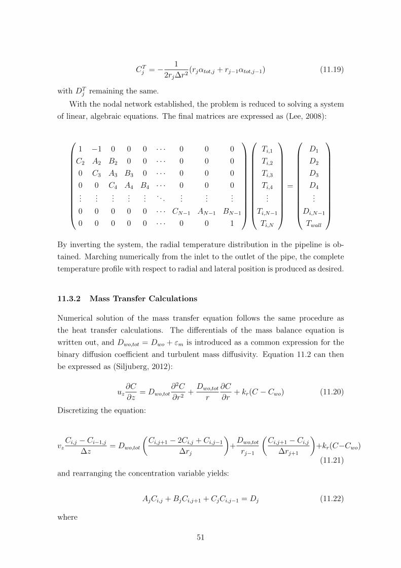
CTj = − 1

2rj∆r2(rjαtot,j + rj−1αtot,j−1) (11.19)

with DTj remaining the same.

With the nodal network established, the problem is reduced to solving a system

of linear, algebraic equations. The final matrices are expressed as (Lee, 2008):

1 −1 0 0 0 · · · 0 0 0

C2 A2 B2 0 0 · · · 0 0 0

0 C3 A3 B3 0 · · · 0 0 0

0 0 C4 A4 B4 · · · 0 0 0...

......

......

. . ....

......

0 0 0 0 0 · · · CN−1 AN−1 BN−1

0 0 0 0 0 · · · 0 0 1

Ti,1

Ti,2

Ti,3

Ti,4...

Ti,N−1

Ti,N

=

D1

D2

D3

D4

...

Di,N−1

Twall

By inverting the system, the radial temperature distribution in the pipeline is ob-

tained. Marching numerically from the inlet to the outlet of the pipe, the complete

temperature profile with respect to radial and lateral position is produced as desired.

11.3.2 Mass Transfer Calculations

Numerical solution of the mass transfer equation follows the same procedure as

the heat transfer calculations. The differentials of the mass balance equation is

written out, and Dwo,tot = Dwo + εm is introduced as a common expression for the

binary diffusion coefficient and turbulent mass diffusivity. Equation 11.2 can then

be expressed as (Siljuberg, 2012):

uz∂C

∂z= Dwo,tot

∂2C

∂r2+Dwo,tot

r

∂C

∂r+ kr(C − Cwo) (11.20)

Discretizing the equation:

vzCi,j − Ci−1,j

∆z= Dwo,tot

(Ci,j+1 − 2Ci,j + Ci,j−1

∆rj

)+Dwo,tot

rj−1

(Ci,j+1 − Ci,j

∆rj+1

)+kr(C−Cwo)

(11.21)

and rearranging the concentration variable yields:

AjCi,j +BjCi,j+1 + CjCi,j−1 = Dj (11.22)

where

51

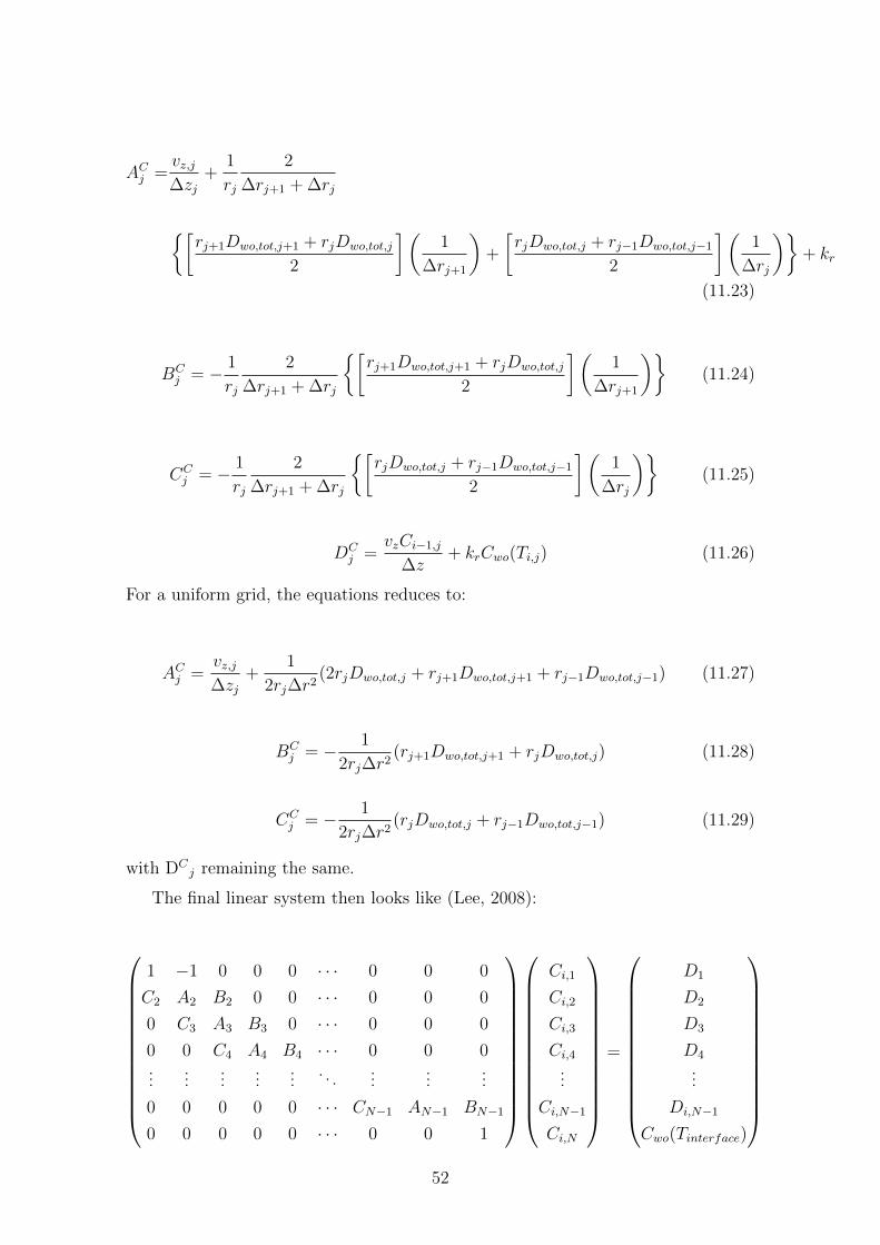
ACj =vz,j∆zj

+1

rj

2

∆rj+1 + ∆rj

{[rj+1Dwo,tot,j+1 + rjDwo,tot,j

2

](1

∆rj+1

)+

[rjDwo,tot,j + rj−1Dwo,tot,j−1

2

](1

∆rj

)}+ kr

(11.23)

BCj = − 1

rj

2

∆rj+1 + ∆rj

{[rj+1Dwo,tot,j+1 + rjDwo,tot,j

2

](1

∆rj+1

)}(11.24)

CCj = − 1

rj

2

∆rj+1 + ∆rj

{[rjDwo,tot,j + rj−1Dwo,tot,j−1

2

](1

∆rj

)}(11.25)

DCj =

vzCi−1,j

∆z+ krCwo(Ti,j) (11.26)

For a uniform grid, the equations reduces to:

ACj =vz,j∆zj

+1

2rj∆r2(2rjDwo,tot,j + rj+1Dwo,tot,j+1 + rj−1Dwo,tot,j−1) (11.27)

BCj = − 1

2rj∆r2(rj+1Dwo,tot,j+1 + rjDwo,tot,j) (11.28)

CCj = − 1

2rj∆r2(rjDwo,tot,j + rj−1Dwo,tot,j−1) (11.29)

with DCj remaining the same.

The final linear system then looks like (Lee, 2008):

1 −1 0 0 0 · · · 0 0 0

C2 A2 B2 0 0 · · · 0 0 0

0 C3 A3 B3 0 · · · 0 0 0

0 0 C4 A4 B4 · · · 0 0 0...

......

......

. . ....

......

0 0 0 0 0 · · · CN−1 AN−1 BN−1

0 0 0 0 0 · · · 0 0 1

Ci,1

Ci,2

Ci,3

Ci,4...

Ci,N−1

Ci,N

=

D1

D2

D3

D4

...

Di,N−1

Cwo(Tinterface)

52

ready to be implemented into the computer program.

11.4 Boundary Conditions

The boundary conditions for heat transfer are as follows:

T =

Tinlet at z = 0 (inlet)

Tb at r = R (radial position of interest)

Tdep at r = rdep (oil/deposit interface)

Twall at r = ri (inner pipe wall)

∂T

∂r= 0 at r = 0 (axial centerline)

where T (K) is the temperature of interest, Tinlet (K) is the inlet temperature, Tb (K)

is the average bulk flow temperature, Tdep (K) is the temperature at the oil/deposit

interface, Twall (K) is the temperature at the wall, Tdep (K) is the temperature at

the solid/liquid interface, z (m) is the distance in the axial direction, r (m) is the

radial distance, R (m) is the radial position at point of interest, ri (m) is the inner

pipe radius and ∂T∂r

(K/m) is the radial temperature gradient.

For mass transfer, the boundary conditions are given as a function of tempera-

ture:

Cinlet = f(Tinlet) at z = 0

Cb = f(Tb) at r = R

Cdep = f(Tdep) at r = R

Cwall = f(Twall) at r = ri

Cmax = f(WAT) at r = R

∂C

∂r= 0 at r = 0

where Cinlet (wt-%) is the concentration of wax dissolved in oil at the inlet, Cb (wt-%)

is the concentration of wax dissolved in the bulk, Cdep (wt-%) is the concentration

at the solid/liquid interface, Cwall (wt-%) is the concentration at the inner pipe wall

and Cmax (wt-%) is the maximum amount of wax dissolved in oil and ∂C∂r

(wt-%/m)

is the radial concentration gradient. The applied solubility equation is presented in

Appendix E.

11.5 Wax Deposit Calculations

As explained in Chapter 6.3, the growth rate and aging of the wax deposit are both

a result of the convective flux of wax molecules from the bulk to the oil/deposit

53

interface (Lee, 2008). The growth rate equals the difference between the convective

flux to the gel deposit surface and the internal diffusion away from the interface,

and is calculated as (Singh, 2000):

(−2πrdep)ρgelFwdrdepdt

= (2πrdep)kM(Cb − Cws(Ti))− (2πrdep)

(−De

dCwsdr

∣∣∣int

)(11.30)

where rsep (m) is the effective flow radius, Fw (-) is the weight fraction of wax in the

deposit, ρgel (kg/m3) is the density of the gel, kM (m/s) is the inner convective mass

transfer coefficient, Cb (wt-%) is the bulk concentration of wax, Cws (wt-%) is the

wax content at the solid/liquid interface, dCws

dris the radial concentration gradient

evaluated at the solid/liquid interface and De (unit) is the effective diffusivity in the

deposit given by Equation (C.3) in Appendix C.

drdepdt

=1

(−2πrdep)ρgelFw

{(2πrdep)kM(Cb − Cws(Ti))− (2πrdep)

(−De

dCwsdr

∣∣∣int

)}(11.31)

The effective flow radius is found as:

rdep(t) = ri −drdepdt

∆t (11.32)

where rsep (m) is the effective flow radius, ri (m) is the inner pipe radius and ∆t (s)

is the time of interest, and the deposit thickness given by:

δ(t) = ri − rdep(t) (11.33)

where δ (m) is the thickness of the deposit layer, ri (m) is the inner pipe radius and

rsep(t) (m) is the effective flow radius at the time of interest.

The aging of the deposit is calculated as follows (Lee, 2008):

πρgel(r2i − rdep2)

dFwdt

= −2πrdep

(−De

dCwsdr

∣∣∣int

)(11.34)

where ρgel (kg/m3) is the density of the deposit, ri (m) is the inner pipe radius, rdep

(m) is the effective flow radius, Fw (-) is the wax fraction in deposit,dFw

dt(s−1) is

the change of wax fraction in deposit with time (aging), De (m2/s) is the effective

diffusivity in the deposit, Cws (wt-%) is the wax content at the solid/liquid interface

and dCws

dr(wt-%/K) is the concentration difference at the solid/liquid interface.

Integrating and rearranging Equation (11.34), the weight fraction of wax to be

used in Equation (11.31) is given as:

54

Fw(t) =2rdepDe

dCws

dr

∣∣∣int

ρgel(r2i − ri2)

(11.35)

with the variables as presented above.

The numerical model requires the convective mass transfer coefficient, kM (m/s),

when calculating the mass transfer rate of wax. This is obtained by the Sherwood

number (Lee, 2008):

Sh =(−2rdep)

dCws

dr

∣∣∣int

Cb − Cdep=

(2rdep)kMDwo

(11.36)

where Sh is the Sherwood number and the variables are as above.

Rearranging Equation (11.36) yields the Equation for the calculation of the mass

transfer coefficient by the MWP:

kM = Dwo

(−2rdep)dCdr

∣∣∣int

Cb − Cdep(11.37)

11.6 Numerical Simulations

The flow conditions and fluid properties applied in the numerical simulations corre-

sponds to the input used in the analytical model, allowing for a direct comparison

of results, as will be done in the subsequent chapter. Because of its complexity, the

numerical model is found to be computational expensive. In the current work, a

pipeline of 1500 meter is chosen simulated. This ensures that the distance at which

the temperature in the viscous sub-layer in the analytical model reaches the WAT

is covered. It should be noted that the numerical model is applicable for any length

and pipeline dimensions and that computer capacity is the only limiting source.

11.6.1 Results

The wax deposit thickness is found to increase with time. The WAT is reached after

49 meter and the maximum deposit thickness is located where the WAT is reached.

From this point on in the pipeline, the deposit thickness is found to decrease. The

deposit thickness profiles obtained by the numerical model are given in Figure 11.1,

where the situation in the pipeline after one, two and seven days are plotted.

The shape of the deposit profiles are again a result of the temperature differ-

ence in the near-wall region being at its maximum where the WAT is reached then

decreasing along the pipeline. The growth rate of the layer decrease with time, in

correspondence with the findings in Chapter 9,

55

Figure 11.1: Deposit thickness profiles after 1 day, 2 days and 7 days obtained bythe numerical model. The maximum deposit thickness is found at 49 meter, wherethe WAT is reached in the near-wall region

56

The deposit thicknesses at 49 meter at the end of the simulated pipeline are

reported in Table 12. The results shows the decreased thickness with axial distance

and a slow growth of the deposit thickness with time. The results will be compared

to the analytical predictions and further commented upon in the subsequent chapter.

In Appendix K, the temperature and concentration profiles in the pipeline after 24

hours are found attached.

Table 12: Deposit thickness values obtained by the analytical model. The thicknessat 49 meter is the maximum deposit thickness and the values at 1500 meter is atthe end of the simulated pipeline..

Deposit Thickness [mm]

Time 49 m 1500 m

1 day 0.77 0.352 days 0.78 0.427 days 0.84 0.53

57

12 Model Comparison

The wax deposit profiles obtained by the analytical and the numerical models will

in the current chapter be compared to external results and to each other. The

numerical results will first be compared to simulations conducted with the same

mathematical model at a different university. The analytical results will then be

compared to wax deposit profiles obtained by a commercial software built upon the

same principles as the analytical model. Finally, the results from the analytical and

the numerical simulations will be compared to each other.

12.1 External Material for Comparison

The wax deposit predictions compared to the simulations conducted in the cur-

rent work, are acquired at the University of Michigan (UiM) and at the Norwegian

University of Science and Technolgoy (NTNU) (Lee, 2008; Kjøraas, 2012). The re-

sults from the UiM are calculated by the mathematical model termed the numerical

model in the current thesis, however, with a different crude oil and under different

flow conditions. Consequently, the deposit thickness predictions from the UiM are

suitable for a qualitative comparison with the numerical results only.

The deposit thickness predictions performed at the NTNU are obtained with

the commercial software HYSYS. HYSYS assumes molecular diffusion as the sole

mechanism for wax deposition using Fick’s law to calculate the mass transfer rate of

wax (Kjøraas, 2012). The concentration gradient is evaluated with the assumption

of thermodynamic equilibrium between the solubility of wax and the actual concen-

tration of wax in solution, hence, the simulations performed in HYSYS are based

upon the same principles as the implemented analytical model.

One distinction between HYSYS and the numerical model, is that HYSYS re-

quires a detailed oil composition as input, whilst a solubility equation considering

the paraffin wax as a pseudo component is applied in the analytical model. The

same oil has been applied in the analytical and in HYSYS, and except from an

assumed oil density of 800 kg/m3 and an inlet temperature of 50 ◦C in the HYSYS

simulations4, the applied fluid properties and flow conditions are identical in the

three simulators (Kjøraas, 2012). The HYSYS results are hence found suitable for

quantitative comparison with the wax deposit predictions obtained in the current

work.

4The oil density is assumed to be 750 kg/m3 and the inlet temperature set to 43◦C in thecurrent work. It should be noted that the inlet temperature only affects where the temperature ofthe fluid reaches the WAT in the pipeline and not the deposit thickness used for comparison.

58

12.2 Comparison of Results

Comparing the results from the UiM with the wax deposit profiles obtained by the

numerical model in the current work, it is observed how the results are in the same

order of magnitude. The deposit thicknesses obtained with the Norne crude oil is

slightly higher than the results reported from the UiM, a deviation that can be

accredited to the differences in flow conditions and applied fluid. The finding is

considered an implication of a correct implementation of the numerical model in

the presented work. The values and differences of the maximum deposit thicknesses

obtained at UiM and with the numerical model are given in Table 13.

Table 13: Maximum deposit thickness in the pipeline calculated by the analyticalmodel at the UiM (Lee, 2008) and NTNU. The results are in the same order of mag-nitude, indicating a correct implementation of the numerical model in the currentwork.

Maximum Deposit Thickness [mm]

Time UiM Numerical Difference

1 day 0.1 0.77 0.672 days - 0.78 -7 days 0.3 0.84 0.54

Comparing the results obtained by the analytical model with the deposit thick-

nesses acquired in HYSYS, the values of the analytical simulations are found to

be well above the results from HYSYS. As the models are based upon the same

principles and the same oil are applied under identical flow conditions, the results

were expected to be more congruent. The deviation may be accredited to the way

the fluid composition is given as input in the models. Kjøraas (2012) reports to

have included only the components up to C45 in the HYSYS simulations, whilst the

solubility equation applied in the analytical model is based on the total composition

of the Norne crude oil covering components up to C100. Since the deviation after

only one day is 3.0 mm and after a week has increased to 11.3 mm, the correctness

of the analytical model is not considered verified by the HYSYS comparison. The

compared results from the analytical simulations and HYSYS are found in Table 14.

The wax deposit thicknesses obtained by the analytical model are found to be

greater than the results obtained by the numerical model. The findings applies

to all three time steps and is in correspondence with the expectations based on

the literature study; the assumption of thermal equilibrium at every point in the

pipeline was expected to result in too high an amount of wax transfer in the viscous

sub-layer and, consequently, a deposit thickness over predicting the situation.

59

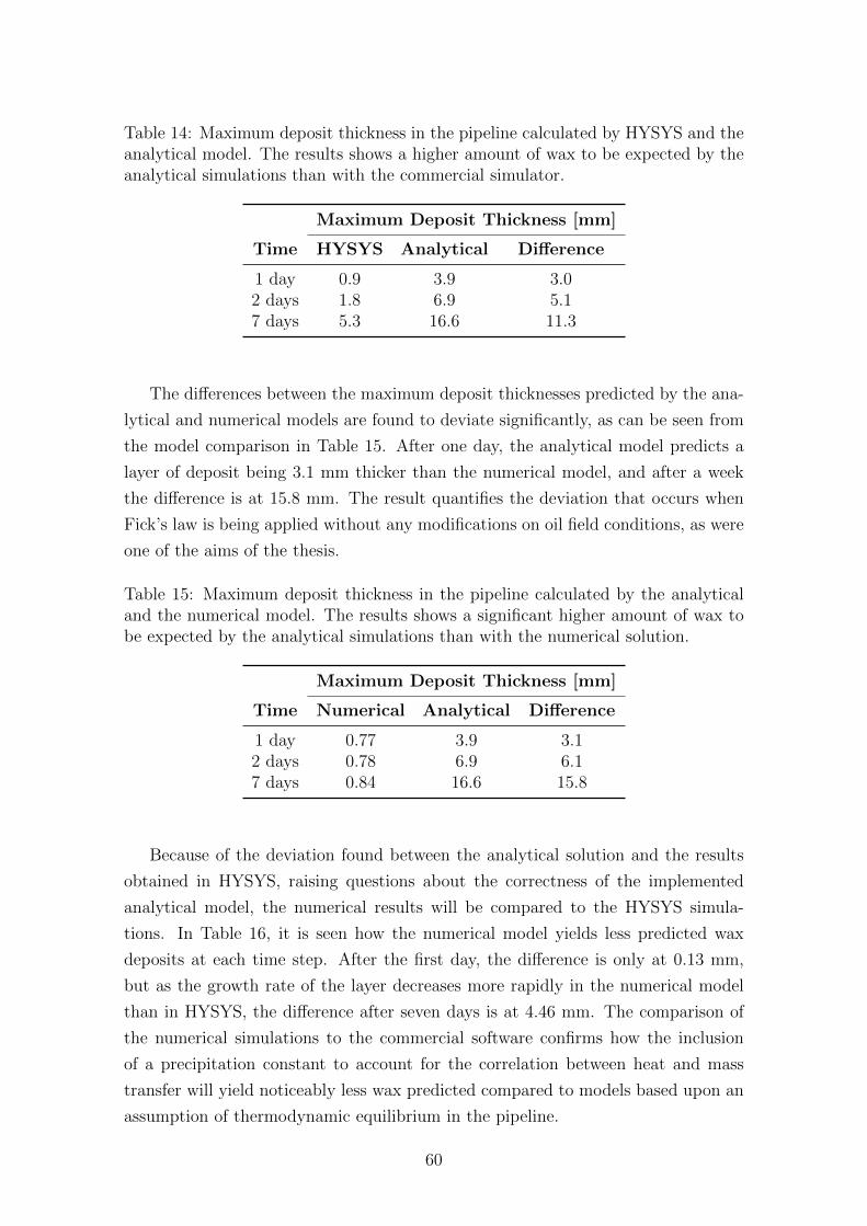
Table 14: Maximum deposit thickness in the pipeline calculated by HYSYS and theanalytical model. The results shows a higher amount of wax to be expected by theanalytical simulations than with the commercial simulator.


Time HYSYS Analytical Difference

1 day 0.9 3.9 3.02 days 1.8 6.9 5.17 days 5.3 16.6 11.3

The differences between the maximum deposit thicknesses predicted by the ana-

lytical and numerical models are found to deviate significantly, as can be seen from

the model comparison in Table 15. After one day, the analytical model predicts a

layer of deposit being 3.1 mm thicker than the numerical model, and after a week

the difference is at 15.8 mm. The result quantifies the deviation that occurs when

Fick’s law is being applied without any modifications on oil field conditions, as were

one of the aims of the thesis.

Table 15: Maximum deposit thickness in the pipeline calculated by the analyticaland the numerical model. The results shows a significant higher amount of wax tobe expected by the analytical simulations than with the numerical solution.


Time Numerical Analytical Difference

1 day 0.77 3.9 3.12 days 0.78 6.9 6.17 days 0.84 16.6 15.8

Because of the deviation found between the analytical solution and the results

obtained in HYSYS, raising questions about the correctness of the implemented

analytical model, the numerical results will be compared to the HYSYS simula-

tions. In Table 16, it is seen how the numerical model yields less predicted wax

deposits at each time step. After the first day, the difference is only at 0.13 mm,

but as the growth rate of the layer decreases more rapidly in the numerical model

than in HYSYS, the difference after seven days is at 4.46 mm. The comparison of

the numerical simulations to the commercial software confirms how the inclusion

of a precipitation constant to account for the correlation between heat and mass

transfer will yield noticeably less wax predicted compared to models based upon an

assumption of thermodynamic equilibrium in the pipeline.

60

Table 16: Maximum deposit thickness in the pipeline calculated by the numericalmodel and HYSYS. The results shows a higher amount of wax to be expected bythe HYSYS simulations than with the numerical solution.


Time Numerical HYSYS Difference

1 day 0.77 0.9 0.132 days 0.78 1.8 1.027 days 0.84 5.3 4.46

The wax deposit profiles for the Norne crude oil obtained in HYSYS are found

in Figure 12.1, showing the deposit thicknesses after 1, 2, 7 and 10 days (Kjøraas,

2012).

Figure 12.1: Wax deposit thickness for the Norne crude oil predicted by the com-mercial software HYSYS (Kjøraas, 2012). The deposit thicknesses are found to behigher than the results from the numerical simulations, but lower than the analyticalresults.

61

13 Shortcomings

The evaluation of the shortcomings in the thesis is divided into shortcomings asso-

ciated with the wax deposit models and shortcomings in the conducted work.

13.1 Shortcomings in the Implemented Models

Neither in the presented models nor in HYSYS is the effect of shear-removal, or the

balance between the deposit layer build up and erosion by the shear effect of the

fluid, included in the wax deposit predictions. Due to high shear at the oil/deposit

interface, the paraffin deposited on the pipeline wall may be sloughed of when the

flow is turbulent (Lee, 2008). Shear-removal is considered a random event and no

model based on first principles are available. If the effect is accounted for i modeling,

empirical tuning parameters are applied (Rønningsen, 2012).

Since the effect of shear-removal is not included in either of the presented models,

the comparative basis of the wax deposit profiles are correct. However, the physical

processes are not correctly described and modeled, representing a severe shortcoming

in the models. The result of including the effect of shear-removal would be a thinner

layer of deposit predicted. The reported deposit thicknesses should therefore be

considered an upper estimate of the actual situation in the pipeline.

Although being a model applied in literature and commercial software, a known

limitation with the analytical model is the area of validity being restricted to laminar

flow conditions. A direct application of the model to normal operative oil field con-

ditions will, per definition, yield incorrect results, an incorrectness being quantified

in the current thesis.

A shortcoming present in both the models, is the applicability of the simulators

being restricted to single phase flow. Oil flow in subsea pipelines is frequently ac-

companied by water and gas, however, neither of the models presented are applicable

for multiphase flow systems (Huang, 2011).

13.2 Shortcomings in the Conducted Work

In the conducted work, the assumption of a constant fluid density and viscosity has

been an applied simplification of the actual situation in the pipeline. In future stud-

ies, the impact of density and viscosity on the wax deposit profiles are recommended

investigated and functions accounting for variations in conditions implemented if

found necessary.

An original idea of the current work, was to compare the results of the analytical

and numerical simulations with what was believed to be a wax deposit profile of

the Norne crude oil applied for verification in previous work (Kjøraas, 2012). The

62

deposit thickness profile in question was acquired from a Statoil presentation held

at NTNU (Aske, 2007). Analyzing the results from Statoil, the rate of deposition

showed to increase with time, contradicting the findings in the current study. It was

confirmed by Statoil that the graphs were not true values from the Norne field, but

an example used for illustration only5 (Stokkenes, 2013b; Stokkenes, 2013c). Hence,

the results from Statoil could neither be used for verification nor falsification of the

implemented work, and the comparison of results obtained with the Norne crude oil

became restricted to three simulators instead of four.

Representing an impracticality just as much as a shortcoming, the numerical

method has shown to be expensive in terms of computer capacity and time required

for a single run. The written computer code is valid for all pipe dimensions, but

for future application, the mathematical model is recommended implemented in a

different language to reduce the runtime and requirement for computer capacity

when performing simulations.

5The deposit thickness was not produced by a combination of the commercial software PVTSimand OLGA which Statoil uses for wax deposit prediction, but was merely a product of power point(Stokkenes, 2013b; Stokkenes, 2013c).

63

14 Summary

A full implementation of an analytical and a numerical model facilitating the predic-

tion of paraffin wax deposits in oil flowing pipelines has been obtained. To account

for temperature variations in the pipeline with position and time, conductive heat

transfer equations have been included for calculation of the radial heat flux through

the wall and the growing layer of wax deposit. As a result, the applicability of the

models are not restricted to flow loops, but valid for real field conditions.

As part of the model construction, five effective thermal conductivity models for

determination of the effective thermal conductivity of the wax deposit have been

evaluated. Based on the structure of the deposit, being a random distribution of

wax and oil, the Effective Medium Theory is found suitable for the wax deposit

modeling.

To evaluate the need for dynamic simulations, the changes in thermal conditions

occurring in the pipeline when wax deposits on the inner pipe wall has been investi-

gated. The presence of deposits is found to add a layer of insulation to the system,

increasing the resistance towards heat flow with an increasing thickness of the layer.

A higher amount of wax in deposit is found to cause less resistance towards heat flow

than a layer of corresponding thickness and a lesser amount of wax. The result is

explained by the thermal conductivity of wax being higher than the thermal conduc-

tivity of oil. The influence of the deposit thickness on the temperature conditions is

found to be greater than the influence of the composition.

As a consequence of the added layer of insulation, the temperature at the oil/de-

posit interface is found to increase with an increasing deposit thickness. With the

temperature at the deposit surface brought closer the bulk flow temperature, the

radial temperature gradient in the pipeline, or the thermal driving force for depo-

sition, decreases. The decreasing driving force for deposition with an increasing

thickness yields a non-linear growth rate of the layer of deposit, requiring dynamic

simulations.

Dynamic wax deposition simulations on a field scale pipeline system under re-

alistic flow conditions have been performed with the analytical and the numerical

models. The results have been compared to external material and to each other.

The numerical model is found to yield results in the same order of magnitude as

what is obtained with the mathematical model at a different university. As different

crude oils under different flow conditions have been applied at the two institutions,

the results are valid for qualitative comparison only. The similarities in the deposit

thickness predictions is taken as an implication of a correct implementation of the

numerical model in the current work.

The analytical simulations have been compared to results obtained with a com-

64

mercial wax deposit predictor. The commercial software is built upon the same

assumptions as the analytical model and simulations are conducted with the same

fluid under identical flow conditions. The analytical model showed to predict a

thicker layer of wax to be expected than was the case with the commercial software.

A possible explanation is the difference in how the fluid composition are given as

input in the two models.

Finally, the analytical and the numerical results were compared. Based on the

literature study, the analytical model was expected to yield a higher amount of wax

deposits than the numerical model. The expectations was found to be true. After

only one day, the analytical model predicted a maximum wax deposit thickness be-

ing 3.1 mm higher than the numerical model and after a week the difference was

increased to 15.8 mm. The results quantifies the differences arising when the numer-

ical model, with its assumption of thermodynamic equilibrium at every point in the

pipeline, is applied, compared to the numerical model which is taking the precipita-

tion kinetics of wax into account. The comparison showed a significant discrepancy

between the expected wax deposit thickness predicted by the two models.

65

15 Future Work

A possible continuation of the current work is to apply the implemented models as

the tools they are meant to be. One option is to investigate the effect of thermal

insulation on the situation in the pipeline. With sufficient knowledge about the

prevailing conditions, the results can be used to evaluate if it will be economical

beneficial to isolate the pipeline or not. On the basis of wax deposit simulations,

pigging schedules for pipelines, with or without insulation, can be prepared, and

costs related to stuck pipe incidents and chemical assistance can be sought for. The

final product could be a report where recommendations for a field development

project, based upon the collected information, is presented.

Before applying the analytical model in any field development project or plan-

ning of operational activity, the area of validity should be extended to the turbulent

flow regime. As it is implemented today, the analytical model serves as the compar-

ative basis it was supposed to be, but it is not recommended applied without any

modifications. One possibility could be to include the turbulent mass diffusivity as

given by Prandtl mixing length theory in the existing computer code and perform

a new evaluation of the method.

An extension of the current work, could be to include the momentum equation

in the implemented models, allowing for dynamic simulations of the axial pressure

drop and the wall shear stress throughout the pipeline. A different direction of study

could be to explore the combination of heat and mass transfer with hydrodynamics

to extend the applicability of the models to multiphase oil/water flow.

66

A References

Aiyejina, A., a. C. D. P., Pilgrim, A., and Sastry, M. Wax formation

in oil pipelines: A critical review. International Journal of Multiphase Flow 37

(2011), 671–694.

Ajienka, J., and Ikoku, C. Criteria for the Design of Waxy Crude Oil Pipelines:

Maximum Pump (Horsepower) Pressure Requirement. Petroleum Science and En-

gineering 13 (1995), 87–94.

Armenante, P. M., and Kirwan, D. J. Mass Transfer to Microparticles in

Agitated Systems. Chemical Engineering Science 21 (2003), 393–408.

Aske, N. Wax - A flow assurance challenge. Guest lecture at NTNU, Statoil

(2007).

Awad, M., and Muzychka, Y. Effective property models for homogeneous

two-phase flow. Experimental Thermal and Fluid Science 33 (2008), 106–113.

Azevedo, L., and Teixeira, A. A Critical Review of the Modeling of Wax

Deposition Mechanisms. Petroleum Science and Technology 21 (2003), 393–408.

Benall, A., Maurel, P., Agassant, J. F., Darbouret, M., Avril, G.,

and Peuriere, E. Wax Deposition in Pipelines: Flow-Loop Experiments and

Investigations on a Novel Approach. SPE 115293, Society of Petroleum Engineers

(2008).

Bunthebarth, G., and Jobmann, M. On Thermal Conductivity of 2-

Component Systems. Presentation, Annual Meeting of the German Geophysical

Society (2008).

Burger, E. D., Perkins, T. K., and Striegler, J. H. Studies of Wax

Deposition in the Trans Alaska Pipeline. Journal of Petroleum Technology 33(6)

(1981), 1075–1086.

Dirksen, J., and Ring, T. Fundamentals of Crystallization: Kinetic Effects

on Particle Size Distribution and Morphology. Chemical Engineering Science 46

(1991), 2389–2427.

Ekweribe, C., Civan, F., Lee, H., and Singh, P. Effect of System Pressure

on Restart Conditions of Subsea Pipelines. SPE 115672, Society of Petroleum

Engineers (2008).

67

Frigaard, I., Vinay, G., and Wachs, A. Compressible Displacement of Waxy

Crude Oils in Long Pipeline Startup Flows. Journal of Non-Newtonian Fluid Me-

chanics 147 (2007), 45–64.

Geankoplis, C. Transport Processes and Separation Process Principles, vol. 4.

2003.

Gudmundsson, J. Grunnleggende enhetsoperasjoner i produksjon av olje og

gass. Compendium, NTNU Institutt for petroleumsteknologi og anvendt geofysikk

(2009).

Gudmundsson, J. S. Unpublished Material. 2012.

Hayduk, W., and Minhas, B. S. Correlations for Prediction of Molecular

Diffusivities in Liquids. The Canadian Journal of Chemical Engineering 60(2)

(1982), 295–299.

Huang, Z. Application of the Fundamentals of Heat and Mass Transfer to the

Investigation of Wax Deposition in Subsea Pipelines. PhD thesis, University of

Michigan, 2011.

Incropera, F., Dewitt, D., Bergman, T. L., and Lavine, A. Fundamentals

of Heat and Mass Transfer, vol. 7. 2011.

Kay, J., and Nedderman, R. Fluid mechanics and transfer processes, vol. 1.

1985.

Kennedy, M., and O’Hagan, A. Bayesian calibration of computer models.

Journal of the Royal Statistical Society 63 (2001), 425–464.

Kjøraas, M. Modeling of Wax Deposition in Subsea Pipelines. Project report,

Norwegian University of Science and Technology, 2012.

Labes-Carrier, C., Rønningsen, H., Kolsnes, J., and Leporche., E. Wax

Deposition in North Sea Gas Condensate and Oil Systems: Comparison Between

Operational Experience and Model Prediction . SPE 77573, Society of Petroleum

Engineers (2008).

Lee, H. S. Computational and Rheological Study of Wax Deposit and Gelation in

Subsea Pipelines. PhD thesis, the University of Michigan, 2011.

Leontaritis, K., and Leontaritis, J. Cloud Point and Wax Deposition Mea-

surements Techniques. SPE 80267, Society of Petroleum Engineers (2003).

68

MathWorks. MATLAB. http://www.mathworks.se/products/matlab/, June

2013.

Mirazizi, H. K., W., S., and Sarica, C. Paraffin Deposition Analysis for

Crude Oils under Turbulent Flow Conditions. SPE 159385, Society of Petroleum

Engineers (2012).

O’Hagan, A. Bayesian analysis of computer code inputs: A tutorial. Reliability

Engineering and System Safety 91 (2006), 1290–1300.

Rø nningsen, H. Rheological behavior of gelled, waxy North Sea crude oils.

Journal of Petroleum Science and Engineering 7 (1992), 177–213.

Rønningsen, H. P. Production of Waxy Oils on the Norwegian Continental Shelf:

Experiences, Challenges, and Practices. Energy and Fuels 26 (2012), 4124–4136.

Sarica, C., and Volk, M. Tulsa University Paraffin Deposition Projects. Tech.

rep., University of Tulsa, 2004.

Sculkes, R. Flow Assurance - Why oil companies focus on multiphase transport.

Guest lecture at NTNU, Statoil, 2013.

Serpil, S., and Servet, G. S. Physical Properties of Food, vol. 1. 2006.

Siljuberg, M. The Bulk Precipitation’s Impact on Concentration Driving Force

in Wax Depostion. Project report, Norwegian University of Science and Technology,

2011.

Siljuberg, M. Modelling of Paraffin Wax in Oil Pipelines. Master thesis, Nor-

wegian University of Science and Technology, 2012.

Singh, A., Lee, H., Singh, P., and Sarica, C. SS: Flow Assurance: Validation

of Wax Deposition Models Using Field Data from a Subsea Pipeline. OTC 21641,

The Offshore Technology Conference (2011).

Singh, P., Venkatesan, R., and Fogler, H. S. Formation and Aging of

Incipient Thin Film Wax-Oil Gels. AIChE Journal 46, 5 (2011), 1059–1074.

Stokkenes, A. Personal communication. E-mail, May, 2013b, Statoil.

Stokkenes, A. Personal communication. E-mail, June, 2013c, Statoil.

Stokkenes, A. Wax control. Guest lecture at NTNU, 2013a, Statoil.

Stubsjøen, M. Wax Modeling in Subsea Oil Pipelines. Project report, Norwegian

University of Science and Technology, 2012.

69

Van Driest, E. R. On Turbulent Flow Near a Wall. AIAA Journal Special

Supplement: Centennial of Powered Flight 23 (1956).

Venkatesan, R., and Creek, J. Wax Deposition and Rheology: Progress and

Problems From an Operator’s View. OTC 20668, Offshore Technology Conference

(2010).

Venkatesan, R., and Fogler, H. S. Comments on Analogies for Correlated

Heat and Mass Transfer in Turbulent Flow. AIChE Journal 47, 1 (2001), 6–18.

Villazon, G. M., and Civan, F. Modeling Multiphase Wax Deposition in

Submarine Pipelines After Shut-In, 5. SPE 124725, Society of Petroleum Engineers

(2009).

Wang, J., Carson, J., North, M., and Cleland, D. A new approach to

modeling the effective thermal conductivity of heterogeneous materials. Heat and

Mass Transfer 49 (2006), 3075–3083.

70

B Heat Transfer Coefficient

There are several empirical correlations available to determine the convective heat

transfer coefficient, h (W/m.K), correlations expressing the Nusselt number as a

function of the Reynolds number and the Prandtl number, Nu = f(Re,Pr). Com-

bined with the definition of the Nusselt number, they allow for the calculation of

the convective heat transfer coefficient. Which correlation found suitable for the

situation is dependent upon flow conditions and geometry. Below, four correlations

applicable for turbulent flow in a circular pipe are presented.

B.1 Chilton-Colburn Correlation

The Chilton-Colburn correlation, expressing the local Nusselt number as (Incropera

et al., 2011):

Nu = 0.023Re4/5Pr1/3 (B.1)

where Re is the Reynolds number and Pr is the Prandtl number. The equation is

valid for turbulent flow in a smooth pipe where:

0.7 ≤ Pr ≤ 160

Re ≥ 10000

L

d≥ 10

L (m) is the length of the pipe and d (m) is the inner pipe diameter.

B.2 Dittus-Boelter Correlation

The Dittus-Boelter correlation is a slightly modified version of the Chilton-Colburn

correlation, specifying whether the fluid is subject to cooling or heating (Incropera

et al., 2011):

Nu = 0.023Re4/5Prn (B.2)

where Re is the Reynolds number, Pr is the Prandtl number, n = 0.4 for heating

and n = 0.3 for cooling. Beyond this, the criterions for using the Dittus-Boelter

equation equals the criterions of the Chilton-Colburn correlation.

Because of their simplicity, the Chilton-Colburn and the Dittus-Boelter correla-

tion are widely applied. However, the equations are found to yield errors as large

71

as 25 %, and sometimes more complex correlation are preferred (Incropera et al.,

2011).

B.3 Pethukov Correlation

To reduce the uncertainty related to the value of the heat transfer coefficient cal-

culation in the model, the Pethukov correlation can be applied (Incropera et al.

2011):

Nu =f8RePr

1.07 + 12.7(f8

) 12 (Pr

23 − 1)

(B.3)

where f is the friction factor, Re is the Reynolds number and Pr is the Prandtl

number. The Pethukov correlation is valid when:

0.5 ≤ Pr ≤ 2000

104 < Re < 106

and the friction factor, f, can be obtained by a Moody chart or by (Incropera and

Dewitt, aarstall):

f = 0.0790 ln(Re− 1.64)−2 (B.4)

for flow in the range of

3000 ≥ Re ≥ 5 · 106

B.4 Gnielski Correlation

A modified version of the Pethukov equation is the Gnielski correlation, expressed

as (Incropera and Dewitt, aarstall):

Nu =f8

(Re− 1000)Pr

1 + 12.7(f8

) 12 (Pr

23 − 1)

(B.5)

where the friction factor can be found by a Moody chart or by Equation (B.4). The

correlation is valid when:

0.5 ≤ Pr ≤ 2000

3000 < Re < 5 · 106

72

Applying one of the more recent correlations, such as the Pethukov equation or the

Gnielinski equation, can reduce the uncertainty of the heat transfer coefficient value

to less than 10 % (Incropera and Dewitt, aarstall). Making use of a more complex

correlation in the wax deposit model will result in a more computational demanding

computer code.

In the wax deposit models, the Dittus-Boelter correlation is chosen applied,

because of its validity under the simulated flow conditions and its simplicity. As

part of a future sensitivity analysis, the influence of the heat transfer coefficient

correlation on the wax deposit prediction is recommended addressed.

73

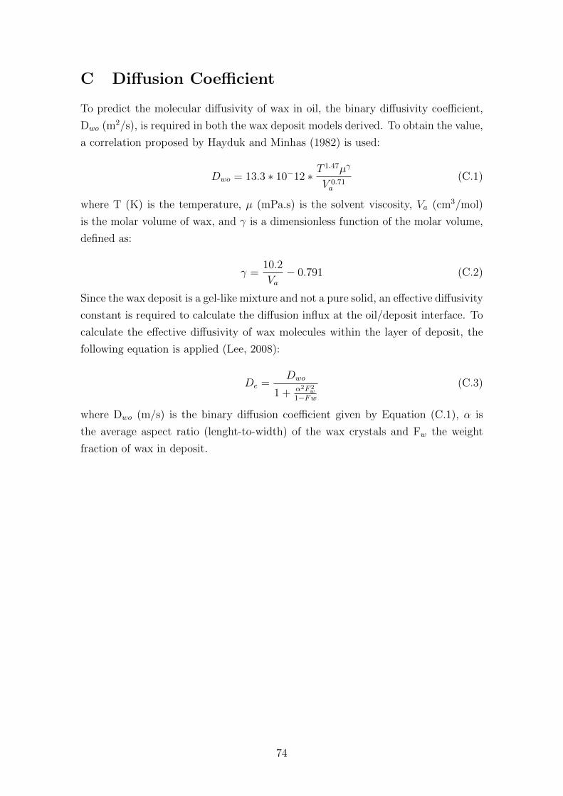
C Diffusion Coefficient

To predict the molecular diffusivity of wax in oil, the binary diffusivity coefficient,

Dwo (m2/s), is required in both the wax deposit models derived. To obtain the value,

a correlation proposed by Hayduk and Minhas (1982) is used:

Dwo = 13.3 ∗ 10−12 ∗ T1.47µγ

V 0.71a

(C.1)

where T (K) is the temperature, µ (mPa.s) is the solvent viscosity, Va (cm3/mol)

is the molar volume of wax, and γ is a dimensionless function of the molar volume,

defined as:

γ =10.2

Va− 0.791 (C.2)

Since the wax deposit is a gel-like mixture and not a pure solid, an effective diffusivity

constant is required to calculate the diffusion influx at the oil/deposit interface. To

calculate the effective diffusivity of wax molecules within the layer of deposit, the

following equation is applied (Lee, 2008):

De =Dwo

1 + α2F 2w

1−Fw

(C.3)

where Dwo (m/s) is the binary diffusion coefficient given by Equation (C.1), α is

the average aspect ratio (lenght-to-width) of the wax crystals and Fw the weight

fraction of wax in deposit.

74

D Precipitation Rate Constant

During precipitation, new particles are created by nucleation events (Dirksen and

Ring, 1991). To account for precipitation kinetics in the concentration profile cal-

culations, a precipitation rate constant is included in the numerical model. The

precipitation rate constant, or growth rate of wax nucleus in the supersaturated so-

lution, is a function of temperature, varying in the pipeline with time and position.

With diffusion assumed to be the rate determining process for particle growth,

the growth rate of precipitated wax particles is given by (Dirksen and Ring, 1991):

G = kdApρn(C − Cws) = kr(C − Cws) (D.1)

where G (m/s) is the growth rate of the precipitated particles, kd (s−1) is the mass

transfer rate from bulk to individual nucleus surface, Ap (m2) is the surface area of a

nucleus, ρn (kg/m3) the nuclei number density, C (kg/m3) is the wax concentration

at the point of interest Cws (kg/m3) is the solubility limit of wax molecules at a

given temperature and kr (s−1) is the precipitation rate constant. The mass transfer

rate from bulk to individual nucleus surface can be found as (Lee, 2008):

kd =ShpDwo

dp(D.2)

where Shp is the Sherwood number for micro particles, Dwo (m2/s) is the binary

diffusion coefficient of wax in oil found by the correlation of Hayduk and Minhas

(1981), and dp (m) i the diameter of the nucleus. Using a mass transfer coefficient

correlation for micro particles (Armenante and Kirwan, 1989):

Shp = 2 + 0.52Re0.52Sc1/3 (D.3)

.

where Re is the Reynolds number and Sc is the Schmidt number and combining

Equation (D.1)-(D.3), an expression for the precipitation rate constant is obtained:

kr =ShpApρn

dpDwo (D.4)

with the variables as above.

The viscosity is calculated from the Arrhenius equation (Lee, 2008):

µ = µcloudexp[EAri

(1

T− 1

Tcloud

)](D.5)

where µcloud (Pa.s) is the dynamic viscosity at the cloud point temperature, EA

(J/mol) is the activation energy, ri (m) is the inner pipe radius and T (K) is the

75

temperature at the point of interest.

Combining Equation (D.4)-(D.5) and taking the ratio between the precipitation

rate constant at any given temperature and the precipitation rate constant at the

cloud point temperature, the precipitation rate constant can be found as:

krkr,cloud

=

(T

Tcloud

)1.47

exp[γEAri

(1

T− 1

Tcloud

)](D.6)

where kr (s−1) is the precipitate rate constant at any temperature of interest, kr,cloud

is the precipitate rate constant at the wax appearance temperature, T (K) is the

temperature of interest, Tcloud is the wax appearance temperature, γ is the dimen-

sionless parameter found by Equation (C.2), EA (J/mol) is the activation energy

and ri (m) is the inner pipe diameter.

The only adjustable parameter in Equation (D.7), is the precipitation rate con-

stant at the wax appearance temperature. Based upon experiments conducted by

Huang (2011), kr,cloud = 1.4 s−1 is applied in the current thesis. Hence, the equation

implemented in the numerical model is:

kr = 1.4

(T

Tcloud

)1.47

exp[γEAri

(1

T− 1

Tcloud

)](D.7)

76

E Applied Solubility Function

To calculate the concentration profiles in both wax deposition models, a temperature

dependent solubility equation is applied. The solubility equation is an empirical

correlation estimating the fraction of wax forming components in the oil, considering

the paraffin as a pseudo component. Since the equation is integrated in the models,

no detailed input of the paraffin distribution is required in either of the models.

The oil applied in the simulations of the current thesis is acquired by Statoil at

the Norne field in the North Sea. The solubility equations for the Norne Crude Oil

is derived by Siljuberg (2012), and given as:

C(T ) = 0.0007T 2 + 0.00989T + 1.7706 (E.1)

where C (wt-%) is the concentration of wax and T (◦C) is the temperature at the

point of interest. The wax appearance temperature of the Norne crude oil is 39◦C

(Aske, 2007).

77

F Simulation Input

Table 17: Input values applied in the simulations.

Variable Symbol Value Unit

Inner pipe diameter d 0.3048 m

Wall Thickness ∆rwall 0.012 m

Pipe length L 2000 m

Ambient Temperature Tsea 5 ◦C

Inlet Temperature Tinlet 41 ◦C

Average Flow Velocity u 2 m/s

Density of Oil ρoil 750 kg/m3

Density of Wax ρwax 750 kg/m3

Dynamic Viscosity of Oil µoil 0.5 mPa.s

Activation Energy EA 37700 J/mol

Molecular Volume Va 430 cm3/mol

Heat Capacity of Oil Cp 2300 J/kg.K

Aspect Ratio of Wax Crystal α 3 -

Thermal Conductivity of Oil koil 0.1 W/m.K

Thermal Conducitivity of Wax kwax 0.25 W/m.K

Thermal Conductivity of Pipe kpipe 0.20 W/m.K

Precipitation Rate at WAT kr,cloud 1.4 s−1

Overall Heat Transfer Coefficient U 20 W/m2K

Time step ∆t 60 min

Number of Steps in Radial direction nj 100 -

Number of Steps in Axial Direction ni 10000 -

78

Table 18: Variables calculated in the simulations.

Variable Symbol Value Unit

Reynolds Number Re 91440 -

Prandtl Number Pr 11.5 -

Inner Heat Coefficient hi 922 W/m2K

Outer Heat Coefficient ho 20.7 W/m2K

79

G Effective Thermal Conductivity Models

Figure G.1: Schematic representation of the structure of the five effective thermalconductivity models evaluated for application in the wax deposit models. The heatflow is assumed to be in the vertical direction (Wang et al., 2006).

80

H Heat Resistance Contribution

Figure H.1: The inner heat resistance contribution to the total thermal resistanceis found to decrease with an increased deposit thickness. A higher wax content indeposit yields less reduction.

81

Figure H.2: The heat resistance contribution to the total thermal resistance of thelayer of deposit is found to increase with an increased deposit thickness. A higherwax content in deposit causes a higher increase.

82

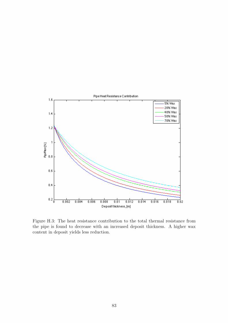
Figure H.3: The heat resistance contribution to the total thermal resistance fromthe pipe is found to decrease with an increased deposit thickness. A higher waxcontent in deposit yields less reduction.

83

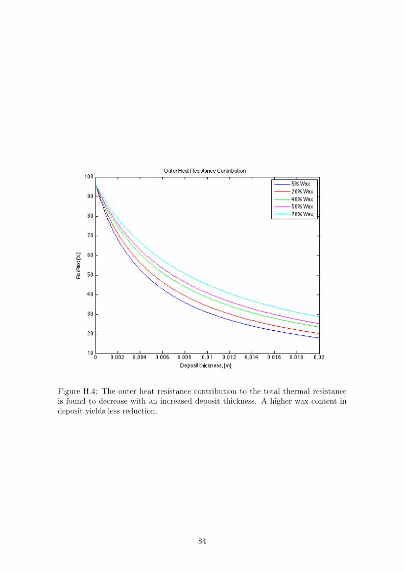
Figure H.4: The outer heat resistance contribution to the total thermal resistanceis found to decrease with an increased deposit thickness. A higher wax content indeposit yields less reduction.

84

I Temperature Profiles

Figure I.1: The temperature at the oil/deposit interface is found to increase with anincreased wax deposit thickness. The increase is higher with a higher wax contentin deposit.

85

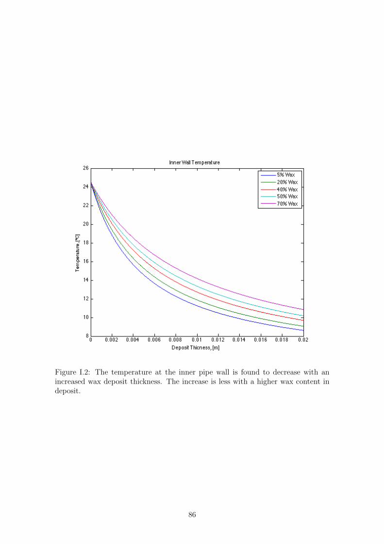
Figure I.2: The temperature at the inner pipe wall is found to decrease with anincreased wax deposit thickness. The increase is less with a higher wax content indeposit.

86

Figure I.3: The temperature at the outer pipe wall is found to decrease with anincreased wax deposit thickness. The increase is less with a higher wax content indeposit.

87

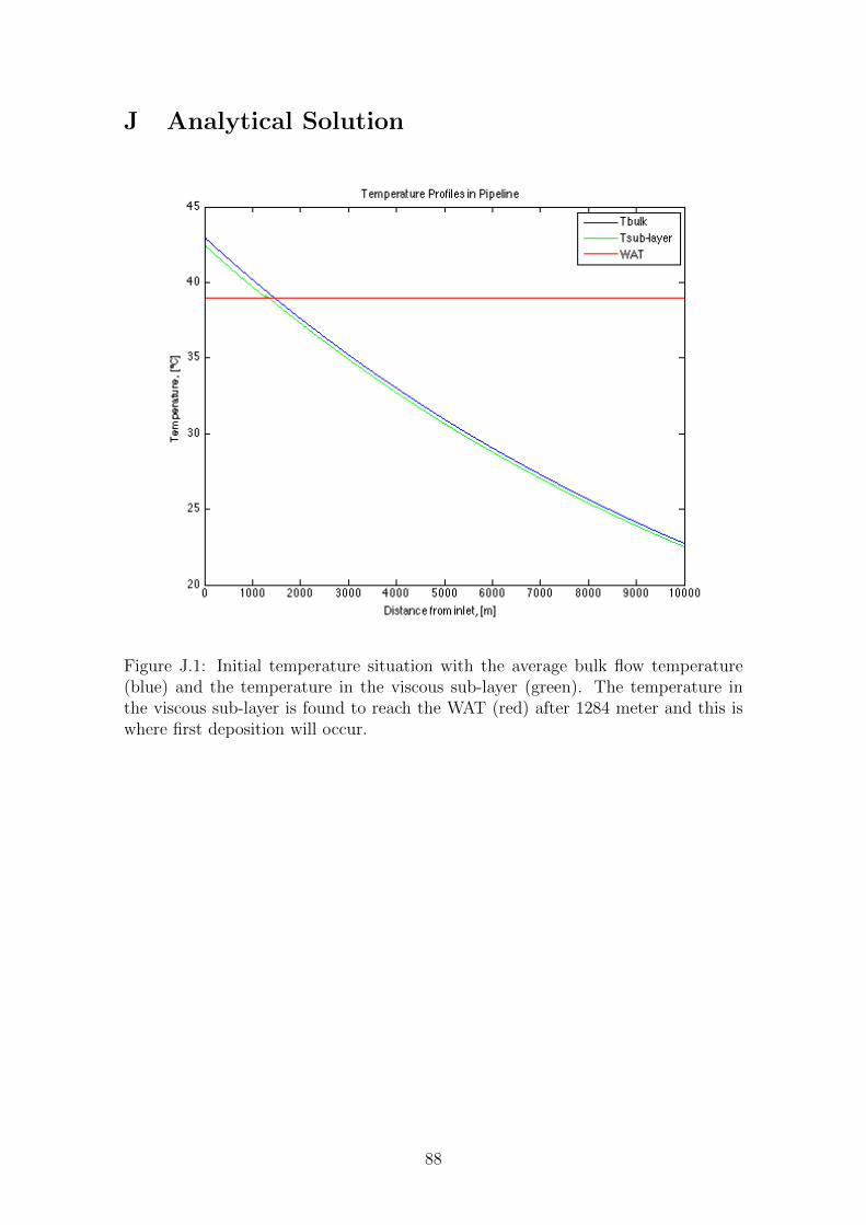
J Analytical Solution

Figure J.1: Initial temperature situation with the average bulk flow temperature(blue) and the temperature in the viscous sub-layer (green). The temperature inthe viscous sub-layer is found to reach the WAT (red) after 1284 meter and this iswhere first deposition will occur.

88

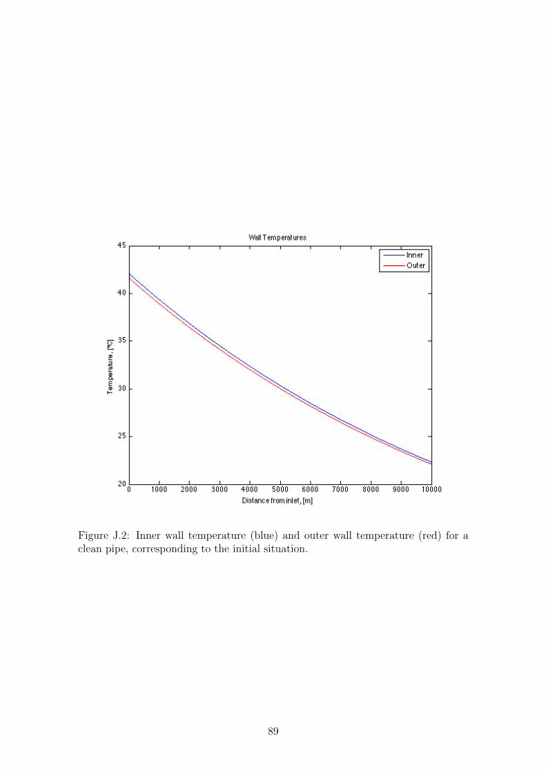
Figure J.2: Inner wall temperature (blue) and outer wall temperature (red) for aclean pipe, corresponding to the initial situation.

89

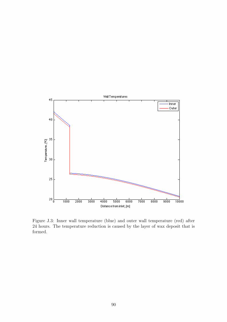
Figure J.3: Inner wall temperature (blue) and outer wall temperature (red) after24 hours. The temperature reduction is caused by the layer of wax deposit that isformed.

90

Figure J.4: Temperature difference across the viscous sub-layer after 24 hours. Themaximum temperature difference is at 1284 meter, where the WAT is reached, ex-plaining why the maximum deposit thickness is encountered here.

91

Figure J.5: Deposit surface temperature profiles after 1 day (blue), 2 days (green)and 7 days (pink) in a section of the pipe. The temperature at the deposit surfaceis found to increase with an increasing deposit thickness.

92

K Numerical Solution

Figure K.1: Temperature profile in the pipeline after 24 hours obtained by thenumerical model. The temperature in the near wall region is observed to be lowerthan the temperature in the bulk flow.

93

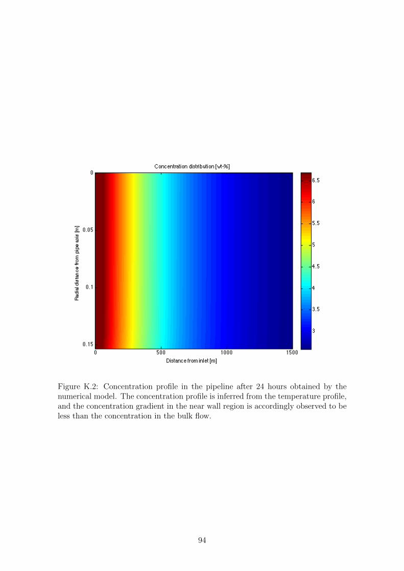
Figure K.2: Concentration profile in the pipeline after 24 hours obtained by thenumerical model. The concentration profile is inferred from the temperature profile,and the concentration gradient in the near wall region is accordingly observed to beless than the concentration in the bulk flow.

94

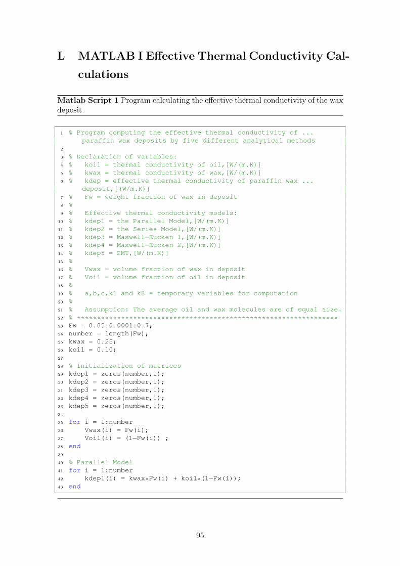
L MATLAB I Effective Thermal Conductivity Cal-

culations

Matlab Script 1 Program calculating the effective thermal conductivity of the waxdeposit.

1 % Program computing the effective thermal conductivity of ...paraffin wax deposits by five different analytical methods

2

3 % Declaration of variables:4 % koil = thermal conductivity of oil,[W/(m.K)]5 % kwax = thermal conductivity of wax,[W/(m.K)]6 % kdep = effective thermal conductivity of paraffin wax ...

deposit,[(W/m.K)]7 % Fw = weight fraction of wax in deposit8 %9 % Effective thermal conductivity models:

10 % kdep1 = the Parallel Model,[W/(m.K)]11 % kdep2 = the Series Model,[W/(m.K)]12 % kdep3 = Maxwell−Eucken 1,[W/(m.K)]13 % kdep4 = Maxwell−Eucken 2,[W/(m.K)]14 % kdep5 = EMT,[W/(m.K)]15 %16 % Vwax = volume fraction of wax in deposit17 % Voil = volume fraction of oil in deposit18 %19 % a,b,c,k1 and k2 = temporary variables for computation20 %21 % Assumption: The average oil and wax molecules are of equal size.22 % *****************************************************************23 Fw = 0.05:0.0001:0.7;24 number = length(Fw);25 kwax = 0.25;26 koil = 0.10;27

28 % Initialization of matrices29 kdep1 = zeros(number,1);30 kdep2 = zeros(number,1);31 kdep3 = zeros(number,1);32 kdep4 = zeros(number,1);33 kdep5 = zeros(number,1);34

35 for i = 1:number36 Vwax(i) = Fw(i);37 Voil(i) = (1−Fw(i)) ;38 end39

40 % Parallel Model41 for i = 1:number42 kdep1(i) = kwax*Fw(i) + koil*(1−Fw(i));43 end

95

1 % Series Model2 for i = 1:number3 kdep2(i)=1/((Fw(i)./kwax)+((1−Fw(i))./koil));4 end5

6 % Maxwell−Eucken 1 (ME1) with oil as the continuous phase and ...wax as the dispersed phase

7 for i = 1:number8 kdep3(i) = ...

(koil*Voil(i)+kwax*Vwax(i)*(3*koil/(2*koil+kwax)))./...9 (Voil(i)+Vwax(i)*((3*koil)/(2*koil+kwax)));

10 end11

12 % Maxwell−Eucken 2 (ME2) with wax as the continuous phase and ...oil as the dispersed phase

13 for i = 1:number14 kdep4(i) = ...

(kwax*Vwax(i)+koil*Voil(i)*(3*kwax/(2*kwax+koil)))./...15 (Vwax(i)+Voil(i)*((3*kwax)/(2*kwax+koil)));16 end17

18 % Effective Medium Theory (EMT) Model19 for i = 1:number20

21 a = −2*(Vwax(i)+Voil(i));22 b = 2*(Vwax(i)*kwax+Voil(i)*koil)−Voil(i)*kwax−Vwax(i)*koil;23 c = kwax*koil*(Vwax(i)+Voil(i));24 k1 = −b/(2*a) + sqrt(bˆ2−4*a*c)/(2*a);25 k2 = −b/(2*a) − sqrt(bˆ2−4*a*c)/(2*a);26

27 if k1 ≥ 028 kdep5(i) = k1;29 else30 kdep5(i) = k2;31 end32 end

96

M MATLAB II Thermal Resistance

Matlab Script 2 Program calculating the thermal resistance in the pipeline.

1 % Program calculating the thermal resistance in the pipeline2

3 % Declaration of variables:4 % d = inner pipe diameter, [m]5 % dr wall = wall thickness, [m]6 % dz = differential in axial direction, [m]7 % rd = effective pipe radius, [m]8 % ri = inner pipe radius, [m]9 % ro = outer pipe radius, [m]

10 %11 % Ad = area of wax deposit (at solid/liquid interface), [mˆ2]12 % Ai = inside area of pipe, [mˆ2]13 % Ao = outside area of pipe, [mˆ2]14 %15 % Alm d = log mean area of deposit, [mˆ2]16 % Alm p = log mean area of pipe, [mˆ2]17 %18 % q = heat transfer rate (heat flux), [W]19 %20 % hi = inner convective heat coefficient21 % ho = outer convective heat coefficient22 %23 % Ri = inner resistance24 % Rd = resistance of deposit25 % Rp = resistance of pipe26 % Ro = outer resistance27 % Rtot = total resistance28 %29 % u = flow velocity, [m/s]30 % mu = oil viscosity [mPs.s]31 % Utot init = overall heat transfer coefficient, [W/mˆ2.K]32 % rho oil = oil density, [kg/mˆ3]33 % Cp = heat capacaty of oil, [J/kg.K]34 %35 % Fw = weight fraction of wax in deposit36 %37 % koil = thermal conductivity of oil38 % kwax = thermal conductivity of wax39 % kpipe = thermal conductivity of pipe40 %41 % kdep = effective thermal conductivity of deposit42 %43 % Vwax = volume of wax in deposit44 % Voil = volume of oil in deposit45 %46 % a,b,c,k1 and k2 = temporary variables for computation47 % Assumption: The oil and wax molecules are of equal size.48 % *****************************************************************

97

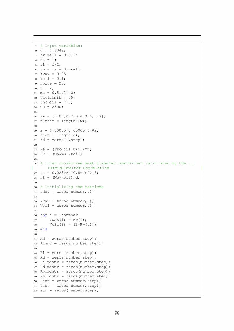
1 % Input variables:2 d = 0.3048;3 dr wall = 0.012;4 dz = 1;5 ri = d/2;6 ro = ri + dr wall;7 kwax = 0.25;8 koil = 0.1;9 kpipe = 20;

10 u = 2;11 mu = 0.5*10ˆ−3;12 Utot init = 20;13 rho oil = 750;14 Cp = 2300;15

16 Fw = [0.05,0.2,0.4,0.5,0.7];17 number = length(Fw);18

19 ∆ = 0.00005:0.00005:0.02;20 step = length(∆);21 rd = zeros(1,step);22

23 Re = (rho oil*u*d)/mu;24 Pr = (Cp*mu)/koil;25

26 % Inner convective heat transfer coefficient calculated by the ...Dittus−Boelter Correlation

27 Nu = 0.023*Reˆ0.8*Prˆ0.3;28 hi = (Nu*koil)/d;29

30 % Initializing the matrices31 kdep = zeros(number,1);32

33 Vwax = zeros(number,1);34 Voil = zeros(number,1);35

36 for i = 1:number37 Vwax(i) = Fw(i);38 Voil(i) = (1−Fw(i));39 end40

41 Ad = zeros(number,step);42 Alm d = zeros(number,step);43

44 Ri = zeros(number,step);45 Rd = zeros(number,step);46 Ri contr = zeros(number,step);47 Rd contr = zeros(number,step);48 Rp contr = zeros(number,step);49 Ro contr = zeros(number,step);50 Rtot = zeros(number,step);51 Utot = zeros(number,step);52 sum = zeros(number,step);

98

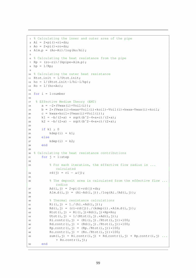
1 % Calculating the inner and outer area of the pipe2 Ai = 2*pi()*ri*dz;3 Ao = 2*pi()*ro*dz;4 Alm p = (Ao−Ai)/log(Ao/Ai);5

6 % Calculating the heat resistance from the pipe7 Rp = (ro−ri)/(kpipe*Alm p);8 hp = 1/Rp;9

10 % Calculating the outer heat resistance11 Rtot init = 1/Utot init;12 ho = 1/(Rtot init−1/hi−1/hp);13 Ro = 1/(ho*Ao);14

15 for i = 1:number16

17 % Effective Medium Theory (EMT)18 a = −2*(Vwax(i)+Voil(i));19 b = 2*(Vwax(i)*kwax+Voil(i)*koil)−Voil(i)*kwax−Vwax(i)*koil;20 c = kwax*koil*(Vwax(i)+Voil(i));21 k1 = −b/(2*a) + sqrt(bˆ2−4*a*c)/(2*a);22 k2 = −b/(2*a) − sqrt(bˆ2−4*a*c)/(2*a);23

24 if k1 ≥ 025 kdep(i) = k1;26 else27 kdep(i) = k2;28 end29

30 % Calculating the heat resistance contributions31 for j = 1:step32

33 % For each iteration, the effective flow radius is ...calculated

34 rd(j) = ri − ∆(j);35

36 % The deposit area is calculated from the effective flow ...radius

37 Ad(i,j) = 2*pi()*rd(j)*dz;38 Alm d(i,j) = (Ai−Ad(i,j))./log(Ai./Ad(i,j));39

40 % Thermal resistance calculations41 Ri(i,j) = 1./(hi.*Ad(i,j));42 Rd(i,j) = (ri−rd(j))./(kdep(i).*Alm d(i,j));43 Rtot(i,j) = Ri(i,j)+Rd(i,j)+Rp+Ro;44 Utot(i,j) = 1/(Rtot(i,j).*Ad(i,j));45 Ri contr(i,j) = (Ri(i,j)./Rtot(i,j))*100;46 Rd contr(i,j) = (Rd(i,j)./Rtot(i,j))*100;47 Rp contr(i,j) = (Rp./Rtot(i,j))*100;48 Ro contr(i,j) = (Ro./Rtot(i,j))*100;49 sum(i,j) = Ri contr(i,j) + Rd contr(i,j) + Rp contr(i,j) ...

+ Ro contr(i,j);50 end

99

N MATLAB III Interface Temperatures

Matlab Script 3 Program calculating the inner pipe wall temperature, the outerpipe wall temperature and the temperature at the deposit surface.

1 % Program calculating the temperatures at the different interfaces.2

3 % Declaration of variables:4 % d = inner pipe diameter, [m]5 % dr wall = pipe wall thickness, [m]6 % rd = effective pipe radius, [m]7 % ri = inner pipe radius, [m]8 % ro = outer pipe radius, [m]9 % mu = dynamic viscosity of oil or condensate, [Pa.s]

10 % rho oil = density of oil, [kg/mˆ3]11 % u = average flow velocity, [m/s]12 % Q = volumetric flow rate, [mˆ3/s]13 % m = mass flow, [kg/s]14 % Cp = heat capacity of oil, [J/kg.K]15 % Tb = bulk temperature, [ C ]16 % Td = temperature at solid/liquid interface, [ C ]17 % Twall in = inner wall temperature, [ C ]18 % Two = outer wall temperature, [ C ]19 % Tsea = ambient temperature, [ C ]20 % Tcheck = control variable, [ C ]21 % Fw = wax fraction in deposit22 % ∆ = deposit thickness, [m]23 % Re = Reynolds number24 % Pr = Prandtl number25 % Nu = Nusselt number26 % Across = pipe cross section area, [mˆ2]27 % Ad = area of wax deposit (at solid/liquid interface), [mˆ2]28 % Ai = inside area of pipe, [mˆ2]29 % Ao = outside area of pipe, [mˆ2]30 % Alm d = log mean area of deposit, [mˆ2]31 % Alm p = log mean area of pipe, [mˆ2]32 % q = heat transfer rate (heat flux), [W]33 % hi = inner convective heat coefficient, [W/mˆ2.K]34 % ho = outer convective heat coefficient, [W/mˆ2.K]35 % koil = thermal conductivity of oil, [W/(m.K)]36 % kwax = thermal conductivity of wax, [W/(m.K)]37 % kdeposit = thermal conductivity of deposit, [W/(m.K)]38 % kpipe = thermal conductivity of pipe, [W/(m.K)]39 % Ri = inner resistance, [W/(mˆ2.K)]40 % Rd = resistance of deposit, [W/(mˆ2.K)]41 % Rp = resistance of pipe, [W/(mˆ2.K)]42 % Ro = outer resistance, [W/(mˆ2.K)]43 % Rtot = total resistance, [W/(mˆ2.K)]44 % frac, thick = loop counters (for iteration)45 % ******************************************************************

100

1 % Assigning input values:2 d = 0.3048;3 dr wall = 0.012;4 dz = 1;5 Tsea = 5;6 Tb = 53;7 u = 2;8 U = 20;9 rho oil = 750;

10 Cp = 2300;11 mu = 0.5*10ˆ−3;12

13 kwax = 0.25;14 koil = 0.1;15 kpipe = 20;16

17 ∆ = 0.00001:0.00001:0.02;18 Fw = [0.05,0.2,0.4,0.5,0.7];19 thick = length(∆);20 frac = length(Fw);21 ri = d/2;22 ro = ri + dr wall;23 Across = pi()*riˆ2;24 Q = u*Across;25 m = Q*rho oil;26

27 Re = (rho oil*u*d)/mu;28 Pr = (Cp*mu)/koil;29 Nu = 0.023*Reˆ0.8*Prˆ0.3;30 hi = (Nu*koil)/d;31

32 % Initialization of matrices33 kdeposit = zeros(1,frac);34 diffTd = zeros(1,frac);35 diffTwi = zeros(1,frac);36 diffTwo = zeros(1,frac);37 diffTch = zeros(1,frac);38 rd = zeros(1,thick);39 Ad = zeros(1,thick);40 Alm d = zeros(1,thick);41 Rd = zeros(frac,thick);42 Rtot = zeros(frac,thick);43 q = zeros(frac,thick);44 Td = zeros(frac,thick);45 Twi = zeros(frac,thick);46 Two = zeros(frac,thick);47 Tcheck = zeros(frac,thick);48 ∆Td = zeros(frac,thick);49 ∆Tp = zeros(frac,thick);

101

1 Ao = 2*pi()*ro*dz;2 Alm p = (Ao−Ai)/log(Ao/Ai);3

4 R = 1/U;5 Ri = 1/(hi*Ai);6 Rp = (ro−ri)/(kpipe*Alm p);7 hp = 1/Rp;8 ho = 1/(R−1/hi−1/hp);9 Ro = 1/(ho*Ao);

10

11 for j = 1: frac12 for i = 1:thick13 rd(1,i) = ri − ∆(1,i);14 Ad(1,i) = 2*pi()*rd(1,i)*dz;15 Alm d(1,i) = (Ai−Ad(1,i))./log(Ai./Ad(1,i));16

17 % Effective Medium Theory (EMT)18 a = −2*(Vwax(i)+Voil(i));19 b = 2*(Vwax(i)*kwax+Voil(i)*koil)−Voil(i)*kwax−Vwax(i)*koil;20 c = kwax*koil*(Vwax(i)+Voil(i));21 k1 = −b/(2*a) + sqrt(bˆ2−4*a*c)/(2*a);22 k2 = −b/(2*a) − sqrt(bˆ2−4*a*c)/(2*a);23

24 if k1 ≥ 025 kdeposit(1,j) = k1;26 else27 kdeposit(1,j) = k2;28 end29

30 Rd(j,i) = (ri−rd(1,i))./(kdeposit(1,j).*Alm d(1,i));31 Rtot(j,i) = Ri+Rd(j,i)+Rp+Ro;32 q(j,i) = (Tsea−Tb)./Rtot(j,i);33

34 Td(j,i) = Tb+(q(j,i).*Ri);35 Twi(j,i) = Td(j,i)+(q(j,i).*Rd(j,i));36 Two(j,i) = Twi(j,i)+(q(j,i).*Rp);37 Tcheck(j,i) = Two(j,i)+(q(j,i).*Ro);38

39 ∆Td(j,i) = Td(j,i)−Twi(j,i);40 ∆Tp(j,i) = Twi(j,i)−Two(j,i);41 diffTd(1,j) = (1−Td(j,thick)./Td(j,1))*100;42 diffTwi(1,j) = (1−Twi(j,thick)./Twi(j,1))*100;43 diffTwo(1,j) = (1−Two(j,thick)./Two(j,1))*100;44

45 end46 end

102

O MATLAB IV Analytical Wax Deposit Model

Matlab Script 4 Analytical wax deposit model.

1 %Program calculating the wax deposit thickness by calling ...associated functions.

2

3 % Declaration of variables:4 % ni = number of steps in radial direction5 % nj = number of steps in aksial direction6 % dr = differential in radial direction7 % dz = differential in lateral direction8 % d = inner pipe diameter, [m]9 % ri = inner pipe radius, [m]

10 % dr wall = pipe wall thickness, [m]11 % ro = outer pipe radius, [m]12 % L = pipe length, [m]13 % Across = pipe cross section area14 % Tsea = ambient temperature, [ C ]15 % Ti = inlet temperature, [ C ]16 % WAT = Wax Appearance Temperature, [ C ]17 % Tsection = temporary storage variabel for calculations, [ C ]18 % mu = dynamic viscosity of oil or condensate, [Pa.s]19 % nu = kinematic viscosity of oil or condensate, [mˆ2/s]20 % rho oil = density of oil, [kg/mˆ3]21 % u = average flow velocity, [m/s]22 % Q = volumetric flow rate, [mˆ3/s]23 % m = mass flow, [kg/s]24 % Re = Reynolds number25 % Pr = Prandtl number26 % Cp = heat capacity of oil27 % hi = inner convective heat transfer coefficient28 % ho = outer convective heat transfer coefficient29 % U = overall heat transfer coefficient30 % koil = thermal conductivity of oil, [W/(m.K)]31 % kwax = thermal conductivity of wax, [W/(m.K)]32 % kpipe = thermal conductivity of pipe, [W/(m.K)]33 % kdeposit = thermal conductivity of deposit, [W/(m.K)]34 % Fw = wax fraction in deposit35 % Va = molecular volume of wax36 % ∆ = initial deposit thickness37 % y = actual distance from pipe wall, [m]38 % f = friction factor39 % u star = friction velocity40 % y p = dimensionless wall distance41 % Tw = inner wall temperature [ C ]42 % qdivA = heat flux, [q/A]43 % *****************************************************************44

45 % Input values:46 L = 10000;47 d = 0.3048;48 nj = L;49 dz = L/nj;

103

1 Tsea = 5;2 Ti = 43;3 u = 2;4 rho oil = 750;5 Cp = 2300;6 Va = 430;7 mu = 0.5*10ˆ−3;8 ∆ = 10ˆ−12;9 Fw = 0.4;

10 y p = 5;11 U = 20;12 WAT = 39;13

14 kwax = 0.25;15 koil = 0.1;16 kpipe = 20;17

18 Re = (rho oil*u*d)/mu;19 Pr = (Cp*mu)/koil;20 Nu = 0.023*Reˆ0.8*Prˆ0.3;21 hi = (Nu*koil)/d;22

23 gamma = 10.2/Va−0.791;24

25 ri = d/2;26 dr wall = 0.012;27 ro = ri + dr wall;28

29 Across = pi()*riˆ2;30 Q = u*Across;31 m = Q*rho oil;32

33 dt = 3600;34 t final = dt*24*7;35 t = 0:dt:t final;36 time = t final/dt;37

38 Vwax = Fw;39 Voil = (1−Fw);40

41 % Effective Medium Theory (EMT)42 a = −2*(Vwax+Voil);43 b = 2*(Vwax*kwax+Voil*koil)−Voil*kwax−Vwax*koil;44 c = kwax*koil*(Vwax+Voil);45 kdep1 = −b/(2*a) + sqrt(bˆ2−4*a*c)/(2*a);46 kdep2 = −b/(2*a) − sqrt(bˆ2−4*a*c)/(2*a);47

48 if kdep1 ≥ 049 kdeposit = kdep1;50 else51 kdeposit = kdep2;52 end

104

1 temperatureL = tempL(Tsea,Ti,U,d,Cp,dz,nj,time,m);2 [depThick,Tdep,Twin,Two,Tsub] = deposit(∆,ri,ro,hi,kpipe,...3 kdeposit,Tsea,temperatureL,dz,nj,time,mu,Va,gamma,WAT,dt,y p,Cp,...4 Re,U,rho oil,Pr,u);

Matlab Script 5 Function calculating the average bulk flow temperature.

1 function temperatur = tempL(Tsea,Ti,U,d,Cp,dz,nj,time,m)2

3 temperatur = zeros(time,nj);4 temperatur(:,1) = Ti;5

6 for i = 1:time7 Tsection = Ti;8

9 for j = 2:nj10 temperatur(i,j) = Tsea + ...

(Tsection−Tsea)*exp((−U*pi()*d*dz)/(m*Cp));11 Tsection = temperatur(i,j);12 end13 end14

15 end

Matlab Script 6 Function calculating the temperature in viscous sub-layer.

1 function [Tsub,y] = tempSub(rho,Pr,mu,u,y p,q,Tw,Cp,Re)2

3 f = 0.305/Reˆ0.25;4 u star = u*sqrt(f/8);5

6 Tw p = Tw*(rho*Cp*u star)/(−q);7

8 if y p ≤ 59 T p = Tw p + Pr*y p;

10 elseif y p > 5 | | y p < 3011 T p = Tw p + (5*Pr + 5*log(0.2*Pr*y p+(1−Pr)));12 else13 T p = Tw p + (5*Pr + 5*log(1+5*Pr) + 2.5*log(y p/30));14 end15

16 Tsub = T p*(−q)/(rho*Cp*u star);17 y = (y p*mu)/(rho*u star);18

19 end

105

Matlab Script 7 Function calculating the deposit thickness and the temperaturesat the inner pipe wall, the outer pipe wall and at the deposit surface.

1 function [depThick,Tdep,Twin,Two,Tsub] = ...2 deposit(thickness,ri,ro,hi,kpipe,kdep,Tsea,tempBulk,dz,...3 nj,time,mu,Va,gamma,WAT,dt,y p,Cp,Re,U,rho,Pr,u)4

5 Tdep = zeros(time,nj);6 Twin = zeros(time,nj);7 Two = zeros(time,nj);8 Tcheck = zeros(time,nj);9 Tsub = zeros(time,nj);

10

11 Ain = 2*pi()*ri*dz;12 Ao = 2*pi()*ro*dz;13 Alm p = (Ao−Ain)/log(Ao/Ain);14

15 Rpipe = (ro−ri)/(kpipe*Alm p);16 hpipe = 1/Rpipe;17 R = 1/U;18 ho = 1/(R−1/hi−1/hpipe);19 Rout = 1/(ho*Ao);20

21 Ad = zeros(time,nj);22 Alm d = zeros(time,nj);23

24 Roil = zeros(time,nj);25 Rdep = zeros(time,nj);26 Rtot = zeros(time,nj);27

28 q = zeros(time,nj);29

30 rdep = zeros(time,nj);31 rdep(1,:) = ri − thickness;32 dr = zeros(time,nj);33

34 depThick = zeros(time,nj);35 depThick(1,:) = thickness;36

37 conc dep = zeros(time,nj);38 conc sub = zeros(time,nj);39

40 Roil(1,:) = 1/(hi*Ain);41 Rtot(1,:) = Roil(1,1)+Rpipe+Rout;

106

1 for j = 1:nj2 q(1,j) = (Tsea − tempBulk(1,j))/Rtot(1,1);3 Twin(1,j) = tempBulk(1,j)+(q(1,j)*Roil(1,1));4 Two(1,j) = Twin(1,j)+(q(1,j)*Rpipe);5 Tcheck(1,j) = Two(1,j)+(q(1,j)*Rout);6 Tsub(1,j) = tempSub(rho,Pr,mu,u,y p,q(1,j),Twin(1,j),Cp,Re);7 end8

9 for i = 2:time10 for j = 1:nj11

12 if depThick(i−1,j) ≤ thickness;13

14 Alm d(i,j) = 0;15

16 Roil(i,j) = 1/(hi*Ain);17 Rtot(i,j) = Roil(i,j)+Rpipe+Rout;18

19 q(i,j) = (Tsea−tempBulk(i,j))./Rtot(i,j);20

21 Twin(i,j) = tempBulk(i,j)+(q(i,j).*Roil(i,j));22 Two(i,j) = Twin(i,j)+(q(i,j).*Rpipe);23 Tcheck(i,j) = Two(i,j)+(q(i,j).*Rout);24 [Tsub(i,j),dr(i,j)] = ...

tempSub(rho,Pr,mu,u,y p,q(i,j),Twin(i,j),Cp,Re);25

26 if Tsub(i,j) < WAT27

28 conc dep(i,j) = 0.0007*Twin(i,j)ˆ2 + 0.00989*Twin(i,j) + ...1.7706;

29 conc sub(i,j) = 0.0007*Tsub(i,j)ˆ2 + 0.00989*Tsub(i,j) + ...1.7706;

30

31 depThick(i,j) = (13.3*10ˆ−12*(Twin(i,j)ˆ1.47*muˆgamma)/...32 Vaˆ.71.*(conc sub(i,j)−conc dep(i,j))/(dr(i,j)*100)).*dt;33

34 if depThick(i,j) ≥ ri35 fprintf('The pipe is clogged after %d hours/days at %d ...

meter\n', i,j);36 return37 end38

39 rdep(i,j) = ri − depThick(i,j);40 Ad(i,j) = 2*pi()*rdep(i,j)*dz;41 end

107

1 else2 Alm d(i,j) = (Ain−Ad(i−1,j))./log(Ain/Ad(i−1,j));3

4 Roil(i,j) = 1./(hi.*Ad(i−1,j));5 Rdep(i,j) = (ri−rdep(i−1,j))./(kdep.*Alm d(i,j));6 Rtot(i,j) = Roil(i,j)+Rdep(i,j)+Rpipe+Rout;7

8 q(i,j) = (Tsea−tempBulk(i,j))./Rtot(i,j);9

10 Tdep(i,j) = tempBulk(i,j)+(q(i,j).*Roil(i,j));11 Twin(i,j) = Tdep(i,j)+(q(i,j).*Rdep(i,j));12 Two(i,j) = Twin(i,j)+(q(i,j).*Rpipe);13 Tcheck(i,j) = Two(i,j)+(q(i,j).*Rout);14 [Tsub(i,j),dr(i,j)] = tempSub(rho,Pr,mu,u,y p,q(i,j),...15 Tdep(i,j),Cp,Re);16

17 conc dep(i,j) = 0.0007*Tdep(i,j)ˆ2 + 0.00989*Tdep(i,j) + 1.7706;18 conc sub(i,j) = 0.0007*Tsub(i,j)ˆ2 + 0.00989*Tsub(i,j) + 1.7706;19

20 depThick(i,j) = depThick(i−1,j) + (13.3*10ˆ−12.*(Tdep(i,j).ˆ...21 1.47.*mu.ˆgamma)./Va.ˆ0.71.*(conc sub(i,j)−conc dep(i,j))./...22 (dr(i,j)*100)).*dt;23 rdep(i,j) = ri − depThick(i,j);24 Ad(i,j) = 2*pi()*rdep(i,j)*dz;25

26 if depThick(i,j) ≥ ri27 fprintf('The pipe is clogged after %d hours/days at %d ...

meter\n', i,j);28 return29 end30

31 end32 end33 end34 end

108

P MATLAB Numerical Wax Deposit Model

Matlab Script 8 Numerical Wax Deposition Model.

1 %Program calculating the wax deposit thickness by calling ...associated functions.

2

3 % Declaration of variables:4 % ni = number of steps in axial direction5 % nj = number of steps in radial direction6 % dr = differential in radial direction7 % dz = differential in lateral direction8 % d = inner pipe diameter, [m]9 % ∆Wall = wall thickness, [m]

10 % r = radius at point of interest, [m]11 % ri = inner pipe radius, [m]12 % ro = outer pipe radius, [m]13 % rd = effective flow radius, [m]14 % L = pipe length, [m]15 % Across = pipe cross section area16 % Ad = area of deposit surface, [mˆ2]17 % Ai = inside area of pipe, [mˆ2]18 % Ao = outside area of pipe, [mˆ2]19 % Alm d = log mean area of deposit, [mˆ2]20 % Alm p = log mean area of pipe, [mˆ2]21 % q = heat transfer rate (heat flux), [W]22 % Twi = inner wall temperature, [ C ]23 % Two = outer wall temperature, [ C ]24 % Ti = inlet temperature, [ C ]25 % Td = temperature at deposit surface, [ C ]26 % Tb = average bulk flow temperature, [ C ]27 % Tsea = ambient temperature, [ C ]28 % Tcheck = control variable, [ C ]29 % WAT = Wax Appearance Temperature, [ C ]30 % alpha = thermal diffusivity of wax in oil mixtures, [mˆ2/s]31 % Dwo = mass diffusivity of wax in oil mixtures, [mˆ2/s]32 % mu = dynamic viscosity of oil or condensate, [Pa.s]33 % nu = kinematic viscosity of oil or condensate, [mˆ2/s]34 % rho oil = density of oil, [kg/mˆ3]35 % rho gel = density of wax, [kg/mˆ3]36 % asp = wax crystal aspect ratio37 % Fw = weight fraction of wax in deposit38 % Va = molecular volume of wax, [cmˆ3/mol]39 % gamma = correlation coefficient40 % Cp = specific heat capacity of oil, [J/kg.K]41 % E = activation energy, [J/K.mol]42 % kr c = precipitation rate constant at WAT, [1/s]43 % Q = volumetric flow rate, [mˆ3/s]44 % u = average flow velocity, [m/s]45 % Re = Reynolds number46 % Pr = Prandtl number47 % Nu = Nusselt number48 % U = overall convective heat transfer coefficient, [W/mˆ2.K]49 % hi = inner convective heat transfer coefficient, [W/mˆ2.K]

109

1 % ho = outer convective heat transfer coefficient, [W/mˆ2.K]2 % Rtot = total thermal resistance, [mˆ2.K/W]3 % Ri = inner resistance, [mˆ2.K/W]4 % Rd = resistance of deposit, [mˆ2.K/W]5 % Rp = resistance of pipe, [mˆ2.K/W]6 % Ro = outer resistance, [mˆ2.K/W]7 % k = thermal conductivity,[W/(m.K)]8 % koil = thermal conductivity of oil, [W/(m.K)]9 % kwax = thermal conductivity of wax, [W/(m.K)]

10 % kpipe = thermal conductivity of pipe, [W/(m.K)]11 % kdeposit = thermal conductivity of deposit, [W/(m.K)]12 % dt = time step13 % t = final simlation time, [s]14 % Cw = concentration of wax in solution at the wall, [wt−%]15 % Ci = concentration of wax in solution at the inlet, [wt−%]16 % kr = precipitation rate constant, [1/s]17 % Sc = Schmidt number18 % Sc T = turbulent Schmidt number19 % C = concentration matrix20 % A C = coefficient matrix21 % D C = D−vector22 % gamma = diffusive constant23 % vz p = dimensionless turbulent velocity, Vz+24 % f = friction factor25 % eddyDiffusivity = diffusion rate coefficient, [mˆ2/s]26 % C1 = correlation constant27 % C2 = correlation constant28 % y p = dimensionless distance from wall, y+29 % y1 = dimensionless distance at radius r30 % y2 = dimensionless distance at radius (r+dr)31 % dy = difference between y1 and y232 % dv = dimensionless velocity difference between y1 and y233 % dvdy = derivative of dimensionless velocity to dimensionless ...

distance34 % kr c = precipitaion rate constant at the cloud point ...

temperature, [1/s]35 % Tc = cloud point temperature, or WAT, [ C ]36 % T = temperature at position of interest, [ C ]37 % E = activation energy, [J/mol]38

39 % Input values:40 d = 0.3048;41 ∆Wall = 0.012;42 L = 1500;43 ni = L;44 nj = 100;45 Tsea = 5;46 Ti = 43;47 WAT = 39;48 u = 2;49 U = 20;

110

1 ∆ = 10ˆ−12;2 ri = d/2;3 rd = ri−∆;4 ro = ri+∆Wall;5 kr c = 1.4;6 E = 37700;7 Fw = 0.4;8 Fwi = 0.05;9 kwax = 0.25;

10 koil = 0.1;11 kpipe = 20;12 mu = 0.5*10ˆ−3;13 Va = 430;14 rho oil = 750;15 rho gel = 750;16 Cp = 2300;17 asp = 3;18 gamma=10.2/Va−0.791;19 nu = mu/rho oil;20 Re = u*d/nu;21 alpha = koil/(rho oil*Cp);22 Pr=nu/alpha;23 Nu = 0.023*Reˆ0.8*Prˆ0.3;24 hi = (Nu*koil)/d;25 Across = pi()*riˆ2;26 Q = u*Across;27 dr=ri/nj;28 dz=L/ni;29 Ai = 2*pi()*ri*dz;30 Ao = 2*pi()*ro*dz;31 Alm p = (Ao−Ai)/log(Ao/Ai);32 Rtotal = 1/U;33 Rp = (ro−ri)/(kpipe*Alm p);34 hp = 1/Rp;35 ho = 1/(Rtotal−1/hi−1/hp);36 Ro = 1/(ho*Ao);37 dt = 3600;38 t final = dt*24*7;39 time = t final/dt;40 z=linspace(0,L,ni);41 r=linspace(0,ri,nj);42

43 if true % For folding and cell execution44

45 rdnew = zeros(time+1,ni);46 rdnew(1,:) = rd;47 R=rdnew;

111

1 dmdt = zeros(time,ni);2 ∆ = zeros(time,ni);3 ∆ in = 0;4

5 Fwax = zeros(time+1,ni);6

7 K = zeros(time,ni);8 Dwo = zeros(time,ni);9 dC = zeros(time,ni);

10 dCb = zeros(time,ni);11

12 waxFrac = zeros(time,ni);13 depThickness = zeros(time,ni);14

15 T=zeros(nj,ni,time);16 C=T;17

18 % Calling functions and performing simulations:19 for t = 1:time20

21 T(:,:,t) = ...temperature(ni,nj,ri,rdnew(t,:),ro,nu,Tsea,Ti,alpha,...

22 dr,dz,Fwi,hi,ho,kwax,koil,kpipe,Pr,u,Re);23 kr = kr generator(ni,nj,T(:,:,t),gamma,WAT,kr c,E,Re);24 C(:,:,t) = ...

concentration(ni,nj,rdnew(t,:),nu,Ti,T(:,:,t),mu,Va,...25 gamma,kr,dr,dz,u,Re);26 C(:,:,t) = wat solubility(nj,ni,C(:,:,t),WAT);27

28 for i = 1:ni29 dC(t,i) = C(end,i,t)−C(end−1,i,t);30 dCb(t,i) = C(1,i,t)−C(end,i,t);31

32 if dC(1,i)<033 Fwax(1,i) = Fwi;34 end35

36 if dC(t,i) == 037 Dwo(t,i) = 0;38 else39 K(t,i) = T(end,i,t)+273.15;40 Dwo(t,i) = ...

13.3*10ˆ−12*(K(t,i)ˆ1.47.*muˆgamma)./(Vaˆ0.71);41 end42

43 [Fwax(t+1,i),depThick(t,i),rdnew(t+1,i),Sh(t,i),dFwdt(t,i),...44 drddtout(t,i),De(t,i),kM(t,i)] = FwdepThick(asp,ri,rho gel,...45 dr,dt,rdnew(t,i),Fwax(t,i),Dwo(t,i),dC(t,i),dCb(t,i));46 end47 end

112

Matlab Script 9 Function calculating the temperature profile in the pipeline.

1 function [T] = ...temperature(ni,nj,ri,rd,ro,nu,Tsea,Ti,alpha,dr,dz,Fw,hi,...

2 ho,kwax,koil,kpipe,Pr,u,Re)3

4 % Initializing the temperature grid5 T = zeros(nj,ni);6 T(:,1) = Ti;7 T(nj,1) = Tw(Tsea,Ti,dz,Fw,hi,ho,kwax,koil,kpipe,rd(1,1),ri,ro);8 Tb = zeros(1,ni);9 Tb(1,1) = Ti;

10

11 % Initializing the coefficient matrix12 A T=zeros(nj,nj); A T(nj,nj) = 1; A T(1,1)=1; A T(1,2)=−1;13

14 for j=2:nj−115 % Calculating thermal diffusivities at different radial positions16 alpha1=alpha tot(dr*(j−1));17 alpha2=alpha tot(dr* (j) );18 alpha3=alpha tot(dr*(j+1));19

20 vz=velocity(j*dr,ri,nu,u,Re);21

22 % Writing the coefficient matrix23 A T(j,j−1)=−1/(2*j*drˆ3)*(j*dr*alpha2+(j−1)*dr*alpha1);24 A T(j,j)=vz/dz+1/(2*j*drˆ3)*(2*j*dr*alpha2+(j+1)*dr*alpha3+...25 (j−1)*dr*alpha1);26 A T(j,j+1)=−1/(2*j*drˆ3)*((j+1)*dr*alpha3+j*dr*alpha2);27 end28

29 % Initializing the D−vector30 D T=ones(nj,1); D T(1)=0;31

32 % Iterating along the pipe from inlet to outlet33 for i=2:ni % z−direction34 T(nj,i)=T(nj,i−1);35 T(nj−1,i)=T(nj,i−1);36

37 % Producing the D−vector38 for j=2:nj−139 vz=velocity(j*dr,ri,nu,u,Re);40 D T(j)=T(j,i−1)*vz/dz;41 end42

43 D T(nj) = Tw(Tsea,Tb(1,i−1),dz,Fw,hi,ho,kwax,koil,kpipe,...44 rd(1,i),ri,ro);45

46 % Solving the linear system47 T(:,i)=A T\D T;48 T(1,i)=T(2,i);49 Tb(i)=T(1,i);50 end

113

1 % Sub−function calculating the total thermal diffusivity2 function alpha t = alpha tot(r)3

4 if Re > 40005 Pr T=0.85+0.015/Pr;6 alpha t=alpha+eddyDiffusivity(r,ri,dr,Re)*Pr/Pr T*alpha;7 else8 alpha t = alpha;9 end

10 end11

12 end

114

Matlab Script 10 Function calculating the temperature at the inner wall, the outerwall and at the deposit surface.

1 function Td = Tw(Tsea,Tb,dz,Fw,hi,ho,kwax,koil,kpipe,rd,ri,ro)2

3 Vwax = Fw;4 Voil = 1−Fw;5

6 % Effective Medium Theory (EMT)7 a = −2*(Vwax+Voil);8 b = 2*(Vwax*kwax+Voil*koil)−Voil*kwax−Vwax*koil;9 c = kwax*koil*(Vwax+Voil);

10 kdep1 = −b/(2*a) + sqrt(bˆ2−4*a*c)/(2*a);11 kdep2 = −b/(2*a) − sqrt(bˆ2−4*a*c)/(2*a);12

13 if kdep1 ≥ 014 kdeposit = kdep1;15 else16 kdeposit = kdep2;17 end18

19 Ad = 2*pi().*rd*dz;20 Ai = 2*pi()*ri*dz;21 Ao = 2*pi()*ro*dz;22

23 Alm d = (Ai−Ad)./log(Ai./Ad);24 Alm p = (Ao−Ai)./log(Ao./Ai);25

26 Ri = 1/(hi*Ai);27 Rd = (ri−rd)/(kdeposit.*Alm d);28 Rp = (ro−ri)/(kpipe*Alm p);29 Ro = 1/(ho*Ao);30 Rtot = Ri+Rd+Rp+Ro;31

32 q = (Tsea−Tb)./Rtot;33

34 Td = Tb+(q.*Ri);35 Twall in = Td+(q*Rd);36 Two = Twall in+(q*Rp);37 Tcheck = Two+(q*Ro);38

39 end

115

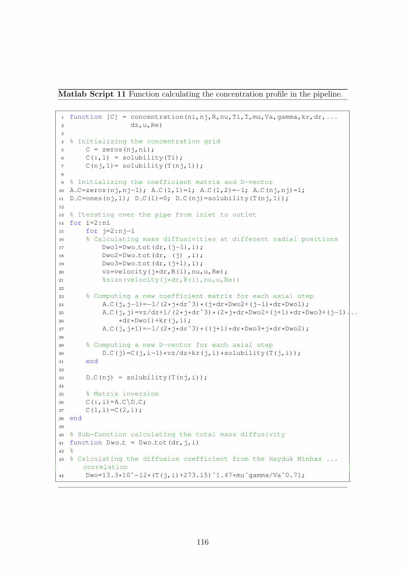
Matlab Script 11 Function calculating the concentration profile in the pipeline.

1 function [C] = concentration(ni,nj,R,nu,Ti,T,mu,Va,gamma,kr,dr,...2 dz,u,Re)3

4 % Initializing the concentration grid5 C = zeros(nj,ni);6 C(:,1) = solubility(Ti);7 C(nj,1)= solubility(T(nj,1));8

9 % Initializing the coefficient matrix and D−vector10 A C=zeros(nj,nj−1); A C(1,1)=1; A C(1,2)=−1; A C(nj,nj)=1;11 D C=ones(nj,1); D C(1)=0; D C(nj)=solubility(T(nj,1));12

13 % Iterating over the pipe from inlet to outlet14 for i=2:ni15 for j=2:nj−116 % Calculating mass diffusivities at different radial positions17 Dwo1=Dwo tot(dr,(j−1),i);18 Dwo2=Dwo tot(dr, (j) ,i);19 Dwo3=Dwo tot(dr,(j+1),i);20 vz=velocity(j*dr,R(i),nu,u,Re);21 %size(velocity(j*dr,R(i),nu,u,Re))22

23 % Computing a new coefficient matrix for each axial step24 A C(j,j−1)=−1/(2*j*drˆ3)*(j*dr*Dwo2+(j−1)*dr*Dwo1);25 A C(j,j)=vz/dz+1/(2*j*drˆ3)*(2*j*dr*Dwo2+(j+1)*dr*Dwo3+(j−1)...26 *dr*Dwo1)+kr(j,i);27 A C(j,j+1)=−1/(2*j*drˆ3)*((j+1)*dr*Dwo3+j*dr*Dwo2);28

29 % Computing a new D−vector for each axial step30 D C(j)=C(j,i−1)*vz/dz+kr(j,i)*solubility(T(j,i));31 end32

33 D C(nj) = solubility(T(nj,i));34

35 % Matrix inversion36 C(:,i)=A C\D C;37 C(1,i)=C(2,i);38 end39

40 % Sub−function calculating the total mass diffusivity41 function Dwo t = Dwo tot(dr,j,i)42 %43 % Calculating the diffusion coefficient from the Hayduk Minhas ...

correlation44 Dwo=13.3*10ˆ−12*(T(j,i)+273.15)ˆ1.47*muˆgamma/Vaˆ0.71;

116

1 if Re > 40002 Sc=nu/Dwo;3 Sc T=0.85+0.015/Sc;4 Dwo t=Dwo+eddyDiffusivity(j*dr,R(i),dr,Re)*Sc/Sc T*Dwo;5 else6 Dwo t = Dwo;7 end8 end9

10 end

Matlab Script 12 Function calculating the solubility of wax in oil.

1 function [solubility] = solubility(T)2 solubility= 0.0007*Tˆ2 + 0.0989*T + 1.7706;3 end

Matlab Script 13 Function calculating the maximum solubility of wax in oil.

1 function [wat sol] = wat solubility(nj,ni,C,Tc)2

3 wat sol = zeros(nj,ni);4 deposited = 0;5

6 solubility Tc= 0.0007*Tcˆ2 + 0.0989*Tc + 1.7706;7

8 for i=1:ni9 for j=1:nj

10 if deposited11 wat sol(j,i) = max(0, solubility Tc − C(j,i));12 else13 wat sol(j,i) = min(C(j,i), solubility Tc);14 end15 end16

17 end

117

Matlab Script 14 Function calculating the precipitation rate constant.

1 function [kr] = kr generator(ni,nj,T,gamma,Tc,kr c,E,Re)2

3 kr = zeros(size(T));4 for j=1:nj5 for i=1:ni6 if Re < 2300 | | T(j,i) > Tc7 kr(j,i) = 0;8 else9 kr(j,i) = ...

kr c*(T(j,i)/Tc)ˆ1.47*exp(((gamma*E)/8.314)*...10 ((1/T(j,i))−(1/Tc)));11 end12 end13 end

Matlab Script 15 Function calculating the eddy diffusivity.

1 function eddyDiff = eddyDiffusivity(r,R,dr,Re)2

3 C1=0.4;4 C2=26;5

6 f=0.305/Reˆ0.25;7 y2=y p(r+dr);8 y1=y p(r);9 dv=vz p(y2)−vz p(y1);

10 dy=y2−y1;11 dvdy=dv/dy;12

13 % Calculating the eddy diffusivity by Van Driests equation14 eddyDiff=(C1.*y p(r)).ˆ2.*(1−exp(−y p(r)/C2)).ˆ2.*dvdy;15

16 % Calculating the dimensionless turbulent velocity by the von Karman17 % correlation18 function vz p = vz p( y p )19 if (y p≤5)20 vz p=y p;21 elseif (5≤y p≤30)22 vz p=5*log(y p)−3.05;23 else24 vz p=2.5*log(y p)+5.5;25 end26 end27

28 % Calculating the dimensionless distance from the wall29 function y p=y p(r)30 y p =(1−r/R)*Re/2*sqrt(f/8);31 end32 end

118

Matlab Script 16 Function calculating the velocity profile.

1 function [velocity] = velocity(r,R,nu,u,Re)2

3 % Laminar flow, Re < 23004 if Re<23005 velocity = 2*u*(1−(r/R)ˆ2);6 return;7

8 % Transition zone 2300 < Re < 40009 elseif Re > 2300 && Re < 4000

10 velocity = 2*u*(1−(r/R)ˆ2);11 return;12

13 % Turbulent flow, Re > 400014 else15 y=R−r;16 f=0.305/Reˆ0.25;17 y p =(1−r/R)*Re/2*sqrt(f/8);18

19 if (y p≤5)20 vz p=y p;21 elseif (5≤y p≤30)22 vz p=5*log(y p)−3.05;23 else24 vz p=2.5*log(y p)+5.5;25 end26

27 velocity=vz p*nu/y*(1−r/R)*Re/2*sqrt(f/8);28 end29 end

119

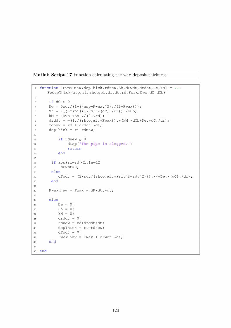
Matlab Script 17 Function calculating the wax deposit thickness.

1 function [Fwax new,depThick,rdnew,Sh,dFwdt,drddt,De,kM] = ...FwdepThick(asp,ri,rho gel,dr,dt,rd,Fwax,Dwo,dC,dCb)

2

3 if dC < 04 De = Dwo./(1+((asp+Fwax.ˆ2)./(1−Fwax)));5 Sh = (((−2*pi().*rd).*(dC)./dr))./dCb;6 kM = (Dwo.*Sh)./(2.*rd);7 drddt = −(1./(rho gel.*Fwax)).*(kM.*dCb+De.*dC./dr);8 rdnew = rd + drddt.*dt;9 depThick = ri−rdnew;

10

11 if rdnew ≤ 012 disp('The pipe is clogged.')13 return14 end15

16 if abs(ri−rd)<1.1e−1217 dFwdt=0;18 else19 dFwdt = (2*rd./(rho gel.*(ri.ˆ2−rd.ˆ2))).*(−De.*(dC)./dr);20 end21

22 Fwax new = Fwax + dFwdt.*dt;23

24 else25 De = 0;26 Sh = 0;27 kM = 0;28 drddt = 0;29 rdnew = rd+drddt*dt;30 depThick = ri−rdnew;31 dFwdt = 0;32 Fwax new = Fwax + dFwdt.*dt;33 end34

35 end

120

Analytical and Numerical Modeling of Paraffin Wax in Pipelines - DiVA

Documents

Transcript of Analytical and Numerical Modeling of Paraffin Wax in Pipelines - DiVA