The Best Cross-Platform Analytic Tools to Monitor Your Web Presence (for Any Budget)

ANALYTIC METHODS FOR SAR IMAGE FORMATIONIN THE PRESENCE OF NOISE AND CLUTTER
By
Huseyin Cagrı Yanık
A Dissertation Submitted to the Graduate
Faculty of Rensselaer Polytechnic Institute
in Partial Fulfillment of the
Requirements for the Degree of
DOCTOR OF PHILOSOPHY
Major Subject: ELECTRICAL ENGINEERING
Approved by theExamining Committee:
Birsen Yazıcı, Dissertation Adviser
Richard J. Radke, Member
John W. Woods, Member
Joyce R. McLaughlin, Member
Rensselaer Polytechnic InstituteTroy, New York
October 2014(For Graduation December 2014)

c© Copyright 2014
by
Huseyin Cagrı Yanık
All Rights Reserved
ii

CONTENTS
LIST OF TABLES . . . . . . . . . . . . . . . . . . . . . . . . . . . . . . . . . vii
LIST OF FIGURES . . . . . . . . . . . . . . . . . . . . . . . . . . . . . . . . ix
ACKNOWLEDGMENT . . . . . . . . . . . . . . . . . . . . . . . . . . . . . . xv
ABSTRACT . . . . . . . . . . . . . . . . . . . . . . . . . . . . . . . . . . . . xvi
1. INTRODUCTION . . . . . . . . . . . . . . . . . . . . . . . . . . . . . . . 1
1.1 Synthetic Aperture Radar . . . . . . . . . . . . . . . . . . . . . . . . 1
1.2 SAR Image Reconstruction Problem . . . . . . . . . . . . . . . . . . 2
1.3 Challenges in SAR Image Formation . . . . . . . . . . . . . . . . . . 3
1.4 The Goal of the Thesis . . . . . . . . . . . . . . . . . . . . . . . . . . 4
1.5 Contributions and Organization of the Thesis . . . . . . . . . . . . . 5
I 7
2. SAR IMAGE RECONSTRUCTION AS A GENERALIZED RADON TRANS-FORM . . . . . . . . . . . . . . . . . . . . . . . . . . . . . . . . . . . . . . 8
2.1 SAR Received Signal Model . . . . . . . . . . . . . . . . . . . . . . . 8
2.2 SAR Image Formation as Inversions of GRTs . . . . . . . . . . . . . . 11
2.2.1 SAR Image Reconstruction by Using the Deterministic Fil-tered -Backprojection . . . . . . . . . . . . . . . . . . . . . . . 12
3. SYNTHETIC APERTURE INVERSION FOR STATISTICALLY NON-STATIONARY TARGET AND CLUTTER SCENES . . . . . . . . . . . . 18
3.1 Related Work . . . . . . . . . . . . . . . . . . . . . . . . . . . . . . . 18
3.2 Statistical Models for Target, Clutter and Noise . . . . . . . . . . . . 21
3.2.1 Non-stationary Target Model . . . . . . . . . . . . . . . . . . 21
3.2.2 Model for the Measurement Noise . . . . . . . . . . . . . . . . 23
3.3 Filter Design Based on MMSE Criteria . . . . . . . . . . . . . . . . . 25
3.4 The Image Reconstruction Algorithm . . . . . . . . . . . . . . . . . . 31
3.4.1 The Estimation of the Space-Varying Spectral Density Function 31
3.4.2 The Steps of the Algorithm . . . . . . . . . . . . . . . . . . . 32
3.4.3 The Computational Complexity of the Algorithm . . . . . . . 33
iii

3.5 Numerical Simulations . . . . . . . . . . . . . . . . . . . . . . . . . . 36
3.5.1 Simulation Setup . . . . . . . . . . . . . . . . . . . . . . . . . 36
3.5.2 Evaluation Method . . . . . . . . . . . . . . . . . . . . . . . . 36
3.5.3 Results . . . . . . . . . . . . . . . . . . . . . . . . . . . . . . . 37
3.5.4 Numerical Simulations with Real Data . . . . . . . . . . . . . 39
3.6 Conclusion . . . . . . . . . . . . . . . . . . . . . . . . . . . . . . . . . 40
4. AN ANALYTIC SAR INVERSION METHOD BASED ON BEST LIN-EAR UNBIASED ESTIMATION . . . . . . . . . . . . . . . . . . . . . . . 49
4.1 Received Signal Model . . . . . . . . . . . . . . . . . . . . . . . . . . 49
4.1.1 Forward Model . . . . . . . . . . . . . . . . . . . . . . . . . . 49
4.1.2 Target, Clutter and Noise Models . . . . . . . . . . . . . . . . 50
4.2 Image Formation based on BLUE Criterion . . . . . . . . . . . . . . . 52
4.2.1 Problem Statement . . . . . . . . . . . . . . . . . . . . . . . . 52
4.2.2 The Bias and Total Variance of BLUE . . . . . . . . . . . . . 53
4.2.3 Derivation of the Imaging Filters . . . . . . . . . . . . . . . . 59
4.3 Numerical Simulations . . . . . . . . . . . . . . . . . . . . . . . . . . 64
4.4 Conclusion . . . . . . . . . . . . . . . . . . . . . . . . . . . . . . . . . 65
II 77
5. FBP-TYPE DIRECT EDGE ENHANCEMENT OF SYNTHETIC APER-TURE RADAR IMAGES . . . . . . . . . . . . . . . . . . . . . . . . . . . 78
5.1 Introduction . . . . . . . . . . . . . . . . . . . . . . . . . . . . . . . . 78
5.2 Forward Modeling and Image Formation . . . . . . . . . . . . . . . . 79
5.3 Segmentation via Edge Detection . . . . . . . . . . . . . . . . . . . . 80
5.4 Direct Segmentation of the SAR Data . . . . . . . . . . . . . . . . . . 82
5.4.1 Derivation of an Edge Detection Filter . . . . . . . . . . . . . 82
5.4.2 Point Spread Function of the Edge Enhanced Reconstruction . 84
5.5 Numerical Experiments . . . . . . . . . . . . . . . . . . . . . . . . . . 84
5.5.1 Synthetic Data Simulations . . . . . . . . . . . . . . . . . . . 84
5.5.2 Civilian Vehicles Dome Data Set . . . . . . . . . . . . . . . . 86
5.6 Conclusion . . . . . . . . . . . . . . . . . . . . . . . . . . . . . . . . . 86
iv

6. ITERATIVE ANALYTIC SAR INVERSION WITH Lp-TYPE REGU-LARIZATION . . . . . . . . . . . . . . . . . . . . . . . . . . . . . . . . . . 92
6.1 Introduction . . . . . . . . . . . . . . . . . . . . . . . . . . . . . . . . 93
6.2 Related Work . . . . . . . . . . . . . . . . . . . . . . . . . . . . . . . 93
6.3 Sparse Signal Recovery Problem . . . . . . . . . . . . . . . . . . . . . 95
6.4 Received Signal, Target, and Noise Models . . . . . . . . . . . . . . . 96
6.5 Analytic SAR Image Formation with Sparsity Promoting Prior Models 98
6.5.1 Problem Definition . . . . . . . . . . . . . . . . . . . . . . . . 98
6.5.2 Approximate Solutions for the Optimization Function . . . . . 99
6.5.2.1 Iterative Reweighted-type Analytic Reconstruction . 99
6.5.2.2 Iterative Shrinkage-type Analytic Reconstruction . . 102
6.6 Numerical Simulations . . . . . . . . . . . . . . . . . . . . . . . . . . 105
6.6.1 Numerical Simulations for IRtA with Synthetic Data . . . . . 105
6.6.1.1 Numerical Simulations for the Under-Sampled Data . 107
6.6.1.2 Numerical Simulations for the Regularly Sampled Data110
6.6.2 Numerical Simulations for IStA with Synthetic Data . . . . . 120
6.6.2.1 Numerical Simulations for the Under-Sampled Data . 120
6.6.2.2 Numerical Simulations for the Regularly Sampled Data124
6.6.3 Numerical Simulations for Lp-norm Regularization with CVDome Data Set . . . . . . . . . . . . . . . . . . . . . . . . . . 131
6.7 Comparison of IRtA and IStA with Other Sparse Recovery Techniques141
6.7.1 Computational Complexity . . . . . . . . . . . . . . . . . . . . 144
6.8 Conclusion . . . . . . . . . . . . . . . . . . . . . . . . . . . . . . . . . 147
7. CONCLUSION . . . . . . . . . . . . . . . . . . . . . . . . . . . . . . . . . 148
BIBLIOGRAPHY . . . . . . . . . . . . . . . . . . . . . . . . . . . . . . . . . 151
APPENDICES
A. METHOD OF THE STATIONARY PHASE . . . . . . . . . . . . . . . . . 167
B. PROOF OF THE LEMMA 1 . . . . . . . . . . . . . . . . . . . . . . . . . 168
C. PROOF OF THE THEOREM 1 . . . . . . . . . . . . . . . . . . . . . . . . 172
D. STATISTICS OF THE RECONSTRUCTED IMAGES . . . . . . . . . . . 176
E. ESTIMATION OF THE SVSD FUNCTIONS . . . . . . . . . . . . . . . . 180
F. A SHORT REVIEW ON BLUE . . . . . . . . . . . . . . . . . . . . . . . . 183
v

G. CALCULATION OF THE HESSIANS FOR CHAPTER 4 . . . . . . . . . 188
G.1 Hessian Matrix for (4.38) . . . . . . . . . . . . . . . . . . . . . . . . . 188
G.2 Hessian Matrix for (4.48) . . . . . . . . . . . . . . . . . . . . . . . . . 188
G.3 Hessian Matrix for (4.53) . . . . . . . . . . . . . . . . . . . . . . . . . 189
H. CONDITIONS FOR THE SPARSE SIGNAL RECOVERY . . . . . . . . . 190
vi

LIST OF TABLES
2.1 Table of Notations Part 1. . . . . . . . . . . . . . . . . . . . . . . . . . 16
2.2 Table of Notations Part 2. . . . . . . . . . . . . . . . . . . . . . . . . . 17
6.1 Table showing the sparsity inducing potential functions, ρ(f) for aninput function f investigated in the thesis. . . . . . . . . . . . . . . . . 98
6.2 The MSE between the true and the reconstructed target image for thefirst five iterations using IRtA for the target scene in Figure 6.1(a). Theminimum values are shown in bold fonts. . . . . . . . . . . . . . . . . . 112
6.3 The relative L2-norm difference between the images reconstructed atevery iteration for the first five iterations using IRtA for the targetscene in Figure 6.1(a). The minimum values are shown in bold fonts. . . 112
6.4 The correlation of the true and the reconstructed target image rangeprofiles for the first five iterations, using IRtA for the target scene inFigure 6.1(a). The maximum values are shown in bold fonts. . . . . . . 113
6.5 The MSE between the true and the reconstructed target image for thefirst five iterations using IRtA for the target scene in Figure 6.6(a). Theminimum values are shown in bold fonts. . . . . . . . . . . . . . . . . . 118
6.6 The relative L2-norm difference between the images reconstructed atevery iteration for the first five iterations using IRtA for the targetscene in Figure 6.6(a). The minimum values are shown in bold fonts. . . 119
6.7 The correlation of the true and the reconstructed target image rangeprofiles for the first five iterations, using IRtA for the target scene inFigure 6.6(a). The maximum values are shown in bold fonts. . . . . . . 119
6.8 The MSE between the true and the reconstructed target image for thefirst five iterations using IStA for the target scene in Figure 6.1(a). Theminimum values are shown in bold fonts. . . . . . . . . . . . . . . . . . 124
6.9 The relative L2-norm difference between the images reconstructed atevery iteration for the first five iterations using IStA for the targetscene in Figure 6.1(a). The minimum values are shown in bold fonts. . . 125
6.10 The correlation of the true and the reconstructed target image rangeprofiles for the first five iterations, using IStA for the target scene inFigure 6.1(a). The maximum values are shown in bold fonts. . . . . . . 125
vii

6.11 The MSE between the true and the reconstructed target image for thefirst five iterations using IStA for the target scene in Figure 6.6(a). Theminimum values are shown in bold fonts. . . . . . . . . . . . . . . . . . 129
6.12 The relative L2-norm difference between the images reconstructed atevery iteration for the first five iterations using IStA for the targetscene in Figure 6.6(a). The minimum values are shown in bold fonts. . . 130
6.13 The correlation of the true and the reconstructed target image rangeprofiles for the first five iterations, using IStA for the target scene inFigure 6.6(a). The maximum values are shown in bold fonts. . . . . . . 130
6.14 The MSE, ∆-norm and the correlation values using IRtA and the CVdome data set for 10 iterations. The tolerance for the IRtA is set to∆-norm less than 1e−3. The row in bold fonts shows the iteration stepat which the algorithm converges. . . . . . . . . . . . . . . . . . . . . . 134
6.15 The MSE, ∆-norm and the correlation values using IStA and the CVdome data set for 20 iterations. The tolerance for the IStA is set to∆-norm less than 1e−3. The row in bold fonts shows the iteration stepat which the algorithm converges. . . . . . . . . . . . . . . . . . . . . . 140
6.16 The MSE, correlation of the range profiles, computation time and theiteration steps at which the algorithms converge for various sparse re-construction techniques. For IRtA and IStA, average values over allpossible potential functions are shown. The computer used for thesesimulations has an Intel Model X3460 8-core CPU clocked at 2.80GHzand 16 GB RAM. All algorithms are implemented in MATLAB. . . . . 145
6.17 The MSE, correlation, computation time and the iteration steps atwhich the algorithms converge for IRtA and IStA with different po-tential functions. The computer used for these simulations has an IntelModel X3460 8-core CPU clocked at 2.80GHz and 16 GB RAM. Allalgorithms are implemented in MATLAB. . . . . . . . . . . . . . . . . 146
viii
LIST OF FIGURES
2.1 Imaging geometries for (a) mono-static SAR where γ(s) is the antennatrajectory, (b) bi-static SAR where γT (s) and γR(s) are the transmit-ter and receiver antenna trajectories, (c) hitchhiker SAR where γRi(s),γRj(s) are receiver trajectories. . . . . . . . . . . . . . . . . . . . . . . . 13
2.2 Iso-range contours for a fixed pulse. Red circle and green square depicttransmitter and receiver, respectively. When intersected with a flattopography, iso-range contours form (a) circles in mono-static SAR (b)ellipsis in bi-static SAR (c) hyperbolas in hitchhiker SAR modalities. . . 14
3.1 (a) Target and (b) radar data, where horizontal and vertical lines cor-respond to slow- and fast-time variables s and t respectively. . . . . . . 39
3.2 (a) Target embedded in clutter and (b) its radar data when SCR is 10dB. 39
3.3 Reconstructed images using (a) the method in [1], (b) with stationarytarget and clutter assumption, (c) non-stationary target and clutterassumption with known SVSD, (d) non-stationary target and clutterassumption with known SVSD when SNR is -20dB and SCR is 10dB. . 41
3.4 Reconstructed images using (a) the method in [1], (b) with stationarytarget and clutter assumption, (c) non-stationary target and clutterassumption with known SVSD, (d) non-stationary target and clutterassumption with known SVSD when SNR is 8dB and SCR is 10dB. . . 42
3.5 Reconstructed images using (a) the method in [1], (b) with stationarytarget and clutter assumption, (c) non-stationary target and clutterassumption with known SVSD, (d) non-stationary target and clutterassumption with known SVSD when SNR is 40dB and SCR is 10dB. . 43
3.6 MSE (vertical axis, in log scale) versus SNR (horizontal axis) averagedover ten reconstructed images for each SNR level using four differentimage reconstruction methods. . . . . . . . . . . . . . . . . . . . . . . . 44
3.7 Reconstructed images using (a) the method in [1], (b) with stationarytarget and clutter assumption, (c) non-stationary target and clutterassumption with known SVSD, (d) non-stationary target and clutterassumption with known SVSD when SCR is -20dB and SNR is 10dB. . 45
3.8 Reconstructed images using (a) the method in [1], (b) with stationarytarget and clutter assumption, (c) non-stationary target and clutterassumption with known SVSD, (d) non-stationary target and clutterassumption with known SVSD when SCR is 8dB and SNR is 10dB. . . 46
ix

3.9 Reconstructed images using (a) the method in [1], (b) with stationarytarget and clutter assumption, (c) non-stationary target and clutterassumption with known SVSD, (d) non-stationary target and clutterassumption with known SVSD when SCR is 40dB and SNR is 10dB. . . 47
3.10 MSE (vertical axis, in log scale) versus SCR (horizontal axis) averagedover ten reconstructed images for each SCR level using four differentimage reconstruction methods. . . . . . . . . . . . . . . . . . . . . . . . 48
3.11 (a) Real SAR image reconstructed from wide-angle SAR data [2] byMethod 1, (b) and Method 4. . . . . . . . . . . . . . . . . . . . . . . . . 48
4.1 The reconstructed images averaged over 10 realizations using (a) thedeterministic FBP, (b) MMSE FBP, (c) BLUE after applying filter Q1,(d) BLUE after applying filter Q2. The SNR is 10dB and SCR is 0 dB. 66
4.2 The reconstructed images averaged over 10 realizations using (a) thedeterministic FBP, (b) MMSE FBP, (c) BLUE after applying filter Q1,(d) BLUE after applying filter Q2. The SNR is 10dB and SCR is 8 dB. 67
4.3 The reconstructed images averaged over 10 realizations using (a) thedeterministic FBP, (b) MMSE FBP, (c) BLUE after applying filter Q1,(d) BLUE after applying filter Q2. The SNR is 10dB and SCR is 16 dB. 68
4.4 The reconstructed images averaged over 10 realizations using (a) thedeterministic FBP, (b) MMSE FBP, (c) BLUE after applying filter Q1,(d) BLUE after applying filter Q2. The SNR is 10dB and SCR is 24 dB. 69
4.5 The reconstructed images averaged over 10 realizations using (a) thedeterministic FBP, (b) MMSE FBP, (c) BLUE after applying filter Q1,(d) BLUE after applying filter Q2. The SNR is 10dB and SCR is 32 dB. 70
4.6 The reconstructed images averaged over 10 realizations using (a) thedeterministic FBP, (b) MMSE FBP, (c) BLUE after applying filter Q1,(d) BLUE after applying filter Q2. The SCR is 10dB and SNR is 0 dB. 71
4.7 The reconstructed images averaged over 10 realizations using (a) thedeterministic FBP, (b) MMSE FBP, (c) BLUE after applying filter Q1,(d) BLUE after applying filter Q2. The SCR is 10dB and SNR is 8 dB. 72
4.8 The reconstructed images averaged over 10 realizations using (a) thedeterministic FBP, (b) MMSE FBP, (c) BLUE after applying filter Q1,(d) BLUE after applying filter Q2. The SCR is 10dB and SNR is 16 dB. 73
4.9 The reconstructed images averaged over 10 realizations using (a) thedeterministic FBP, (b) MMSE FBP, (c) BLUE after applying filter Q1,(d) BLUE after applying filter Q2. The SCR is 10dB and SNR is 24 dB. 74
x

4.10 The reconstructed images averaged over 10 realizations using (a) thedeterministic FBP, (b) MMSE FBP, (c) BLUE after applying filter Q1,(d) BLUE after applying filter Q2. The SCR is 10dB and SNR is 32 dB. 75
4.11 MSE (vertical axis, in dB) versus (a) SNR (horizontal axis) with con-stant SCR level at 10dB and (b) SCR (horizontal axis) with constantSNR level at 10dB averaged over ten reconstructed images using fourdifferent image reconstruction methods. . . . . . . . . . . . . . . . . . . 76
5.1 Imaging scenes used to generate the radar data. . . . . . . . . . . . . . 86
5.2 Enhancement of edges in all directions for the first scene. . . . . . . . . 87
5.3 Enhancement of edges in all directions for the second scene. . . . . . . . 88
5.4 Enhancement of edges in x-direction for scene 2 with µ = [1, 0]. . . . . 88
5.5 Enhancement of edges in y-direction for scene 2 with µ = [0, 1]. . . . . . 89
5.6 Enhancement of edges in x and y-directions for scene 2 with µ1 = [1, 0]and µ2 = [0, 1]. . . . . . . . . . . . . . . . . . . . . . . . . . . . . . . . 89
5.7 Original image reconstructed with FBP. . . . . . . . . . . . . . . . . . . 90
5.8 Enhancement of edges in all directions. . . . . . . . . . . . . . . . . . . 90
5.9 Enhancement of edges along x1 direction, i.e. µ = [1, 0]. . . . . . . . . . 91
5.10 Enhancement of edges along x2 direction, i.e. µ = [0, 1]. . . . . . . . . . 91
6.1 (a) The original and (b) the reconstructed scene using the deterministicFBP with a single realization. SNR is set to 0dB and the Gaussiannoise is added to the data to simulate the measurement noise. . . . . . . 107
6.2 The reconstructed images (a) using the deterministic FBP (initializationof the algorithm); and IRtA after (b) the first, (c) second, (d) third,(e) tenth, and (f) the twentieth iterations when the SNR is 0dB and
ρ(f) = f2
1+f2 for the target in Figure 6.1. . . . . . . . . . . . . . . . . . . 108
6.3 The range profiles of the (a) reconstructed image at the tenth iteration,and (b) the true target scene in Figure 6.1(a). . . . . . . . . . . . . . . 109
6.4 The plots showing (a) the MSE between the original target scene andthe reconstructed target image for each iteration, (b) ∆-norm, (c) cor-
relation of the range profiles when ρ(f) = f2
1+f2 for IRtA and the scene
in Figure 6.1(a). . . . . . . . . . . . . . . . . . . . . . . . . . . . . . . . 110
xi

6.5 Images showing (a) the MSE between original target scene and the re-constructed target image for each iteration, (b) ∆-norm, (c) correlationof the range profiles for the target scene in Figure 6.1(a) with all poten-
tial functions in the order of f2
1+f2 , f 2, log(1 + f 2), f1+f
, f , log cosh(T ),
min(f 2, 2f − 1), f 1/2, f1/2
1+f2−1/2 for IRtA. . . . . . . . . . . . . . . . . . . 111
6.6 (a) The original and (b) the reconstructed scene using the deterministicFBP with a single realization. SNR is set to 0dB and Gaussian noise isadded to data to simulate the additive thermal noise. . . . . . . . . . . 113
6.7 The reconstructed images (a) using the deterministic FBP (initializationof the algorithm); and IRtA (b) after the first, (c) second, (d) third, (e)
tenth, and (f) twentieth iterations when the SNR is 0dB and ρ(f) = f2
1+f2
for the target in Figure 6.6. . . . . . . . . . . . . . . . . . . . . . . . . . 114
6.8 The range profiles of the (a) reconstructed image at the tenth iteration,and (b) the true target scene in Figure 6.6(a). . . . . . . . . . . . . . . 115
6.9 The plots showing (a) the MSE between original target scene and thereconstructed target image for each iteration, (b) ∆-norm, (c) correla-
tion of the range profiles when ρ(f) = f2
1+f2 for IRtA and the scene in
Figure 6.6(a). . . . . . . . . . . . . . . . . . . . . . . . . . . . . . . . . 116
6.10 Images showing (a) the MSE between original target scene and the re-constructed target image for each iteration, (b) ∆-norm, (c) correlationof the range profiles for the target scene in Figure 6.6(a) with all poten-
tial functions in the order of f2
1+f2 , f 2, log(1 + f 2), f1+f
, f , log cosh(T ),
min(f 2, 2f − 1), f 1/2, f1/2
1+f2−1/2 for IRtA. . . . . . . . . . . . . . . . . . . 117
6.11 The reconstructed images (a) using the deterministic FBP (initializationof the algorithm); and IStA (b) after the first, (c) second, (d) third, (e)
tenth, and (f) twentieth iterations when the SNR is 0dB and ρ(f) = f2
1+f2
for the target in Figure 6.1. . . . . . . . . . . . . . . . . . . . . . . . . . 121
6.12 The plots showing (a) the MSE between original target scene and thereconstructed target image for each iteration, (b) ∆-norm, (c) correla-
tion of the range profiles when ρ(f) = f2
1+f2 for IStA and the scene in
Figure 6.1(a). . . . . . . . . . . . . . . . . . . . . . . . . . . . . . . . . 122
6.13 Images showing (a) the MSE between original target scene and the re-constructed target image for each iteration, (b) ∆-norm, (c) correlationof the range profiles for the target scene in Figure 6.1(a) with all poten-
tial functions in the order of f2
1+f2 , f 2, log(1 + f 2), f1+f
, f , log cosh(T ),
min(f 2, 2f − 1), f 1/2, f1/2
1+f2−1/2 for IStA. . . . . . . . . . . . . . . . . . . 123
xii

6.14 The reconstructed images (a) using the deterministic FBP (initializationof the algorithm); and IStA (b) after the first, (c) second, (d) third, (e)
tenth, and (f) twentieth iterations when the SNR is 0dB and ρ(f) = f2
1+f2
for the target in Figure 6.6. . . . . . . . . . . . . . . . . . . . . . . . . . 126
6.15 The plots showing (a) the MSE between original target scene and thereconstructed target image for each iteration, (b) ∆-norm, (c) correla-
tion of the range profiles when ρ(f) = f2
1+f2 for IStA and the scene in
Figure 6.6(a). . . . . . . . . . . . . . . . . . . . . . . . . . . . . . . . . 127
6.16 Images showing (a) the MSE between original target scene and the re-constructed target image for each iteration, (b) ∆-norm, (c) correlationof the range profiles for the target scene in Figure 6.6(a) with all poten-
tial functions in the order of f2
1+f2 , f 2, log(1 + f 2), f1+f
, f , log cosh(T ),
min(f 2, 2f − 1), f 1/2, f1/2
1+f2−1/2 for IStA. . . . . . . . . . . . . . . . . . . 128
6.17 (a) The reconstructed Jeep image via FBP using the entire CV domedata set and (b) the left-bottom corner of the car that is used in corre-lation calculations. . . . . . . . . . . . . . . . . . . . . . . . . . . . . . . 131
6.18 The reconstructed SAR images for the CV dome data set using (a) thedeterministic FBP; and IRtA after (b) the first, (c) second, and (d) thetenth iterations, respectively when the SNR is 20dB and ρ(f) = ∇f . . . 132
6.19 (a) The MSE between the original target scene and the reconstructedtarget image for each iteration, (b) the ∆-norm, (c) the correlation ofthe reconstructed image patch shown in Figure 6.17(b) using IRtA andthe CV dome data set when the SNR is 20dB and ρ(f) = ∇f . . . . . . 133
6.20 The reconstructed SAR images for the CV dome data set using (a) thedeterministic FBP; and IStA after (b) the first, (c) second, and (d) thetenth iterations, respectively when the SNR is 20dB and ρ(f) = ∇f . . . 136
6.21 The reconstructed SAR images for the CV dome data set using IStAafter (a) the twentieth, and (b) the thirtieth iterations, respectivelywhen the SNR is 20dB and ρ(f) = ∇f . . . . . . . . . . . . . . . . . . . 137
6.22 (a) The MSE between the original target scene and the reconstructedtarget image for each iteration, (b) the ∆-norm, (c) the correlation ofthe reconstructed image patch shown in Figure 6.17(b) using IStA andthe CV dome data set when the SNR is 20dB and ρ(f) = ∇f . . . . . . 138
6.23 Images reconstructed using (a) IRtA and (b) IStA at the convergencestep of the algorithms with CV dome data set. IRtA converged at thethird iteration and IStA converged at the eighteenth iteration with thetolerance level of 1e-03 when the SNR is 20dB and ρ(f) = ∇f . . . . . . 139
xiii

6.24 The reconstructed images using the methods (a) BP, (b) IRWLS, (c)IST, (d) LARS, (e) LASSO, and (f) PFP at 30dB SNR. . . . . . . . . . 142
6.25 The reconstructed images with the methods (a) least squares, (b) stage-wise OMP, (c) backprojection, (d) FBP, (e) IRtA, and (f) IStA at 30dBSNR. . . . . . . . . . . . . . . . . . . . . . . . . . . . . . . . . . . . . . 143
xiv

ACKNOWLEDGMENT
I would like to express my sincere gratitude to my dissertation advisor, Prof. Birsen
Yazıcı, for her aspiring guidance, everlasting support, invaluably constructive criti-
cism, patience and encouragement on uncountable occasions during this dissertation
and my entire graduate education years. As my mentor, I hope Prof. Yazıcı will
always be present in my future work.
I would like to acknowledge the members of the dissertation committee, Prof.
Richard J. Radke, Prof. John W. Woods and Prof. Joyce R. McLaughlin for their
time, valuable discussions and productive comments on this work.
I would also like to take this opportunity to express my warm thanks to Kaan
Duman, Nihat Baysal, Deniz Rende and Yasemin Yesiltepe, who have been my
family in Troy. Many thanks to Oguzhan Uyar, Cemal Cagatay Bilgin, Basak Oztan,
Sahin Cem Geyik and Bugra Caskurlu for their great friendship and making the past
five years enjoyable.
Last but not least, I would like to express my deepest love and dedicate this
dissertation to my father Rıza Tevfik Yanık, my mother Pakize Yanık, and my little
brother Hamdullah Yanık, who supported me without any doubt my whole life and
assured me that I can achieve anything.
xv

ABSTRACT
Synthetic Aperture Radar (SAR) is a valuable imaging modality in civil and en-
vironmental monitoring, defense and homeland security applications. This thesis
presents novel analytic and computationally efficient SAR image formation meth-
ods in the presence of noise and clutter using a priori models for target, clutter and
noise.
The first part of the thesis presents statistical SAR inversion methods to
suppress noise and clutter using spatially-varying quadratic priors. We present
a novel class of non-stationary stochastic processes, which we refer to as pseudo-
stationary, to model radar targets and clutter. First, we develop analytic filtered-
backprojection- and backprojection-filtering-type SAR inversion methods based on
the minimum mean square error criterion when the target and the clutter are pseudo-
stationary. Next, we develop an analytic inversion formula based on a best linear
unbiased estimation criterion when the clutter is a pseudo-stationary process.
In the second part of the thesis, we investigate non-quadratic prior models to
represent target scenes. Specifically, we consider edge-preserving prior models. First,
we present a simultaneous analytic, image formation and edge detection method.
Then, we formulate the SAR image reconstruction as non-quadratic optimization
problems. We solve these optimization problems approximately with sequences of
filtered-backprojection operators.
The methods presented in this thesis have the advantages of computational
efficiency, applicability to arbitrary imaging geometries and several different SAR
modalities.
The methods and algorithms derived in this thesis are extensively tested using
high-fidelity simulated data and real SAR data.
xvi

CHAPTER 1
INTRODUCTION
1.1 Synthetic Aperture Radar
Synthetic Aperture Radar (SAR) is a coherent imaging technique used in a
wide range of applications from civil and environmental monitoring to defense and
homeland security. SAR has the advantage of providing rich information, long-range,
all-weather operation and large area coverage.
A typical SAR system involves a source of electromagnetic (EM) illumination
and (a) receiving antenna(s). The movement of the source and/or receiver(s) allows
mathematical synthesis of an image from the backscattered EM waves.
SAR can be used in a variety of modes depending on the number and geomet-
ric configurations of antennas, transmitted waveforms, center frequency and other
operating parameters.
In mono-static SAR configuration, receiving and transmitting antennas are
located on the same platform [3].
In a bi-static SAR, receiving and transmitting antennas are sufficiently far
apart so that the transmitter and the receiver look directions are different [1]. Re-
cently, bi-static configuration has received increasing attention in the context of
passive radar applications.
A multi-static SAR configuration involves three or more sufficiently far apart
antennas that are receiving, transmitting or both [4]. With the recent advances
in unmanned air vehicle (UAV) and microsatellite technologies [5]–[11], there is a
growing interest in multi-static SAR [4], [12]–[15].
Hitchhiker is a novel SAR modality that involves multiple receiving anten-
nas [16]. It takes advantage of ambient EM waves provided by the transmitters
of opportunity to perform radar tasks. Hitchhiker SAR may be useful in urban
areas where there are many transmitters of opportunity such as GSM, TV, Wi-Fi
transmitters.
In addition to these, there are many other SAR modalities that can be derived
1

2
by configuring imaging parameters in space, time, polarization state, frequency etc.
These modalities include the along-track and cross-track interferometric SAR, po-
larimetric SAR to mention a few.
1.2 SAR Image Reconstruction Problem
There are analytical and numerical optimization-based SAR inversion tech-
niques. Analytical techniques are widely used and they are computationally efficient.
However, they cannot accommodate the measurement noise and clutter explicitly.
Moreover, there are limitations to the antenna trajectories. In order some of the
assumptions to hold for image formation with some of these techniques, antennas
need to traverse short, linear trajectories.
The range-Doppler algorithm is the most commonly used analytical method
in SAR image formation [17], [18]. The method is easy to implement and requires
calculation of a matched-filter. However, the method has some limitations since
the ideal matched-filter depends on the location of the target which is unknown
and the calculation of the matched-filter can be computationally burdensome. The
chirp-scaling algorithm [19] offers a solution to the computational load by bypass-
ing some of the interpolation needed for the range-Doppler algorithm via scaling
the chirp signal, which is a special type of transmitted waveform in SAR. There is
also ω-k algorithm that formulates the SAR inversion problem by using the wave
equation [20], [21]. This algorithm is also referred to as the wave number domain
algorithm and performs focusing via Stolt interpolation [22] to deal with the wide
aperture issues inherent with the range-Doppler and chirp-scaling methods. The
polar-format algorithm compensates for the limitations of range-Doppler method
by exploiting the fact that the SAR received signal is collected in a spherical ge-
ometry (polar coordinate system) [23], [24]. Finally, there are backprojection-based
analytic inversion methods [1], [3]. Our research group has been extensively work-
ing on backprojection-based analytic inversion methods from a generalized Radon
transform (GRT) point of view [1], [4], [16], [25]. [25] was the first work in the lit-
erature to incorporate a priori statistical information about the target and clutter
scenes with an analytic inversion method. We consider SAR collected data as a

3
GRT of the scene reflectivity function (representing the scatterers on the ground)
weighted and projected onto some smooth manifolds. Backprojection-based meth-
ods can accommodate arbitrary imaging geometries. In Chapter 2, we describe the
SAR image formation from a GRT point of view.
Numerical optimization-based techniques are a second class of SAR inversion
methods. They use discrete models and can be statistical or deterministic. Nu-
merical optimization-based techniques consider the measurement noise and clutter
present in the scene, however most of the time they are computationally intensive.
Numerical optimization-based methods treat SAR image formation operator as a
forward matrix and attempt to find inverse matrices to form SAR images. Detailed
literature survey on numerical optimization based methods are given in Section 3.1
and Section 6.2.
In this thesis, we wish to develop computationally efficient, backprojection-
based, analytic SAR inversion methods that are robust in the presence of noise
and clutter and use a priori information to accurately characterize SAR target and
clutter scenes.
1.3 Challenges in SAR Image Formation
1- Noise and clutter: The measurement noise and clutter are ubiquitous
in SAR data. The classical SAR image reconstruction techniques, such as matched
filtering, range-Doppler [17] and chirp scaling algorithms [19] do not take into ac-
count noise and clutter, explicitly. Noise and clutter reduce the detectability and
the recognition of targets.
2- Computational efficiency: SAR images cover large swaths. For exam-
ple, a typical TerraSAR-X image of New Orleans area is a 14, 000 × 14, 000-pixel
image. Therefore, SAR is a computationally demanding, large inversion problem.
Fast algorithms are desired to achieve computational efficiency. There are analytical
and numerical optimization-based techniques to address these problems. Analytical
techniques are widely used and they are computationally efficient. However, they
cannot explicitly accommodate noise and clutter. Numerical optimization-based
techniques can use statistical or deterministic models. However, most of the time

4
they are computationally intensive.
3- Use of “accurate” a priori information: The spectral estimation-
based techniques generally require a priori information about clutter and suitable
initialization for the convergence of the algorithms [26]. In the knowledge aided
space-time adaptive processing (KA-STAP) methods, this prior information is col-
lected when there are no targets in the imaging scene and provided as a clutter
covariance matrix to be used as training data. To overcome the requirement on
prior information, parametric techniques are proposed [27]–[29] but they are com-
putationally intensive.
4- Non-stationary nature of clutter and target: Often times, in nu-
merical optimization based methods, measurement noise is modeled to be additive
Gaussian [30]–[34] without any specification on the statistical nature of the target
and the clutter. This induces model-based errors to the reconstructed SAR images
due to non-stationary nature of the target and the clutter in reality.
5- Limited data: SAR systems can be used to operate in multiple modes
such as imaging and ground-moving target imaging. Such systems are referred to
as the interrupted SAR systems. Switching between different operation modes may
result in missing or undersampled data. Moreover, the amount of data collected
for a single acquisition may be very large to transmit and process in real time.
Also, in many practical applications the data may be incomplete to apply analytic
inversion methods, effectively [35]–[38]. Therefore, it is desirable to develop SAR
reconstruction algorithms using limited aperture data.
1.4 The Goal of the Thesis
In this thesis, we wish to develop computationally efficient, analytic image
reconstruction methods that are (1) robust in the presence of noise and clutter; (2)
based on specific a priori information that can accurately characterize SAR target
and clutter scenes.
Towards this goal, the thesis develops the following:
1. A novel class of non-stationary processes to model radar targets and clutter.

5
2. Analytic and computationally efficient inversion methods within the minimum
mean square error (MMSE) and best linear unbiased estimator (BLUE) frame-
works when target and clutter belong to this class of processes.
3. Analytic, iterative and computationally efficient inversion methods using edge-
preserving non-quadratic prior models on radar targets.
1.5 Contributions and Organization of the Thesis
This thesis comprises of two parts. In the first part, we investigate quadratic
priors to model radar targets and clutter. In the second part, we use non-quadratic
priors for the target scenes.
The contributions of this thesis are as follows:
In Chapter 2:
• We briefly describe the SAR image reconstruction problem from a GRT point
of view.
In Chapter 3:
• We develop analytic, computationally efficient solutions to SAR image forma-
tion problem in the presence of noise and clutter. The methods described in
this thesis are of backprojection-type. Therefore, they can be implemented
with the computational complexity of the fast backprojection algorithms [39],
[40].
• We develop a novel class of statistically non-stationary processes to model
radar targets and clutter. We refer to this new family of processes as the
pseudo-stationary processes and they are locally stationary.
• We further show that the stochastic processes that can be represented by using
pseudo-stationary processes are outputs of time-varying convolution filters.
• By using this new family of processes, we develop an FBP-type, analytic SAR
reconstruction method that suppresses noise and clutter based on MMSE cri-
terion. We use MMSE locally which overcomes the over-smoothing effect of
MMSE.

6
• We introduce backprojection-filtering as a novel SAR inversion method.
• Implementation of FBP- and BPF-type noise and clutter suppression meth-
ods require the space-varying spectral density (SVSD) functions for the target
and clutter. We develop an algorithm similar to the one described in [41] to
estimate target and clutter SVSD functions directly from the radar data in
the same chapter.
In Chapter 4:
• We develop an analytic SAR image reconstruction method that suppresses
noise and clutter based on BLUE criterion.
In Chapter 5:
• We describe a novel direct edge-enhancement method that simultaneously re-
constructs images and enhances edges along desired directions. The method
is also capable of smoothing edges along desired directions.
In Chapter 6:
• We use non-quadratic priors to model radar targets.
• We model SAR image formation problem as an Lp-norm constrained mini-
mization problem. We approximate this problem with a sequence of L2-norm
constrained inversion problems.
• We present iterative reweighted- and shrinkage-type algorithms to solve this
non-quadratic optimization problem.
• We use the method described in Chapter 5 to sharpen the reconstructed im-
ages.
• Different than other noise/clutter suppression techniques, Lp-type regulariza-
tion can be applied to limited data.
We demonstrate the performance of the proposed methods with synthetic data
formed by MATLAB, real data from Wide Angle SAR experiment [2] and the Civil-
ian Vehicles (CV) dome data set [42], both provided by the Air Force Research
Laboratories (AFRL). Chapter 6 concludes the thesis.

PART I
7

CHAPTER 2
SAR IMAGE RECONSTRUCTION AS A GENERALIZED
RADON TRANSFORM
In this chapter, we first derive the SAR received signal model starting from the scalar
wave equation. Then, we describe the SAR image formation from a generalized
Radon transform point of view. Finally, we derive a filtered-backprojection type
filter for SAR in a deterministic setting.
2.1 SAR Received Signal Model
For a bi-static SAR system, where transmitting and receiving antennas are
located on different platforms, we model the transmitted EM waves as a time-
varying source jTR(t,x) distributed over an aperture. jTR(t,x) is proportional to
an effective current density on the transmitting antenna and can include arbitrary
waveforms. We assume that the earth’s surface is located at x = [x1, x2,ψ(x1, x2)]
where ψ : R2 → R, is a known smooth function of the ground topography, and
scattering takes place in a thin region near the surface. Throughout this thesis, the
bold Roman, bold italic, and Roman small letters will denote points in R3, R2 and
R, respectively, i.e. x ∈ R2, x3 ∈ R, and x = [x, x3] ∈ R3.
The source term satisfies the scalar wave equation given by:
(∇2 − c−2∂2
t
)uin(t,x) = −jTR(t,x) (2.1)
where ∇ denotes the gradient operator, c is the speed of light in free-space, ∂ is the
partial derivative operator and uin(t,x) is the incident field at time t and location
x. Using the Green’s function
g0(t,x) =δ(t− |x|/c)
4π|x|=
∫e−iω(t−|x|/c)
8π2|x|dω (2.2)
8

9
where ω is the angular frequency. Using the fact that
(∇2 − c−2∂2
t
)g0(t,x) = −δ(t,x) (2.3)
we obtain
uin(t,x) = (g0 ∗ jTR)(t,x) =
∫e−iω(t−|x−y|/c)
4π|x− y|jTR(ω,y)dxωdy, (2.4)
where ∗ denotes the convolution and
jTR(ω,y) =1
2π
∫jTR(t,y)eitωdt (2.5)
is the Fourier transform of jTR.
For a pulsed radar system it is assumed that the pulses are transmitted at
ti and the antenna position at the ith pulse transmission is γ(ti). Let s := ti
denote the time at which a pulse is transmitted. Since the time scale at which
the electromagnetic wave moves is much smaller than the time scale at which the
antenna moves, we refer to s as the slow-time and t as the fast-time. We further
assume that the antenna is small compared with the distance to the scatterers.
Using the far-field expansion we write
|x− y| = |(x− γ(s)) + (γ(s)− y)| ≈ |x− γ(s)|+ (x− γ(s)) · (γ(s)− y) (2.6)
since |γ(s) − y| |x − γ(s)| where x− γ(s) = x−γ(s)|x−γ(s)| is the unit vector in the
direction x− γ(s). Then,
uin(t,x) ≈∫
e−iω(t−|x−γ(s)|/c)
4π|x− γ(s)|jTR(ω, x− γ(s))dωdy, (2.7)
and
jTR(ω, x− γ(s)) = eiω (x−γ(s))·γ(s)/c
∫e−iω (x−γ(s))·y/cjTR(ω,y)dy. (2.8)

10
The Fourier transform (2.8) gives the antenna beam pattern at each fixed
frequency in the far-field. It is seen from (2.7) that the field transmitted by the
antenna is a superposition of the fixed-frequency point sources that are each shaped
by the antenna beam pattern. Using the scalar wave equation for the total field
utot(t,x) we obtain
(∇2 − c−2(x)∂2
t
)utot(t,x) = −jTR(t,x) (2.9)
where c(x) is the speed of the EM wave in the medium. We write total field as
utot(t,x) = uin(t,x) + usc(t,x) (2.10)
and use (2.1)-(2.9) to get
(∇2 − c−2∂2
t
)usc(t,x) = −V (x)∂2
t utot(t,x) (2.11)
where
V (x) =1
c2− 1
c2(x). (2.12)
Here, we refer to V (x) as the ground reflectivity function that contains all the
information related to the scattering nature of the ground.
Under the single-scattering (or Born) approximation utot(t,x) is replaced by
uin(t,x) and solving (2.11), we obtain
uscB (t,x) =
∫g0(t− τ,x− z)V (z)∂2
τuin(τ, z)dτdz, (2.13)
which for the incident field (2.7) becomes
uscB (t,x, s) =
∫e−iω(t−(|x−z|+|z−γ(s)|)/c)
(4π)2|x− z||z− γ(s)|ω2JTR(ω, z− γ(s))V (z)dωdydz. (2.14)

11
2.2 SAR Image Formation as Inversions of GRTs
Under the Born (single scattering) and start-stop approximations, for many
SAR modalities [1], [3], [16] the ideal scattered field data can be modeled as follows:
f(s, t) ≈ F [V ](s, t) :=
∫e−i2πω(t−R(s,x)/c)A(x, s, ω)V (x) dωdx, (2.15)
where ω is the angular frequency, c denotes the speed of light in free-space, A is
a complex amplitude term that includes the antenna beam patterns, transmitted
waveform, geometrical spreading factors, etc. s ∈ [s0, s1] ⊂ R is the slow-time and
t ∈ [t0, t1] ⊂ R is the fast-time.
V (x) is given by
V (x) =1
c2− 1
c2(x)(2.16)
where c(x) is the speed of the EM wave in the scatterer and V (x) is the ground
reflectivity function. V (x) recovered from the backscattered EM waves is called the
SAR image. R(s,x) can be interpreted as the distance between the antennas and
the scatterer at x.
Depending on the SAR modality, the antenna range, R(s,x), takes different
forms.
Rm(s,x) = 2|γ(s)− x| (2.17)
for mono-static SAR [3] where γ(s) denotes the antenna trajectory;
Rb(s,x) = |γT (s)− x|+ |γR(s)− x| (2.18)
for bi-static SAR [1] where γT (s) and γR(s) denote the transmitter and the receiver
antenna trajectories, respectively; and
Rh(s,x) = |γi(s)− x| − |γj(s)− x| (2.19)
for hitchhiker SAR [16] where γi(s) and γj(s) denote the trajectories of the ith and

12
jth receiver antennas, respectively. Note that x = [x, ψ(x)] in (2.17)-(2.19).
For all SAR modalities, it is assumed that for some mA, the amplitude term
A satisfies the symbol estimate [1], [16]:
sup(s,x)∈K
| ∂αω∂βs ∂ρxA(x, s, ω) | ≤ BK,α,β,ρ (1 + |ω|)mA−|α| (2.20)
where K is any compact subset of R×R2, BK,α,β,ρ is a K,α, β,ρ dependent constant,
and ρ is a multi-index. This assumption holds since most SAR modalities involve
waveforms that are slowly varying in frequency domain. This assumption makes the
“forward” operator F , a Fourier Integral Operator (FIO) [43]–[46].
The image of the scene is reconstructed from the data collected from the
measurements of the scattered waves. An FIO can be viewed as a GRT where
the input function is weighted and projected onto some smooth manifolds. SAR
measurement data can be viewed as a GRT of the scene reflectivity function in
which the reflectivity is weighted and projected onto some smooth manifolds. These
manifolds can be circles (mono-static SAR), ellipsis (bi-static SAR) or hyperbolas
(hitchhiker SAR) depending on the imaging geometry assuming a flat topography.
The weighting or filtering is defined by the amplitude term and the smooth
manifolds are defined by the phase function of the FIO which is determined by
the antenna configuration. If the amplitude function, A(x, ω, s) equals to 1, which
corresponds to an isotropic antenna radiating a delta-like impulse and compensating
for the geometric spreading factors, then the FIO simply projects the input function
onto the manifolds defined by its phase term as given in (2.17)-(2.19). Figures 2.2
(a)-(c) illustrate the smooth manifolds onto which the scene reflectivity function is
projected assuming that the topography is flat.
2.2.1 SAR Image Reconstruction by Using the Deterministic Filtered
-Backprojection
Since the forward operator F in (2.15) is a Fourier integral operator, an image
T of the target scene T is formed by another Fourier integral operator K that is of

13
(a)
(b)
(c)
Figure 2.1: Imaging geometries for (a) mono-static SAR where γ(s) isthe antenna trajectory, (b) bi-static SAR where γT (s) and γR(s) are thetransmitter and receiver antenna trajectories, (c) hitchhiker SAR whereγRi(s), γRj(s) are receiver trajectories.

14
(a) (b)
(c)
Figure 2.2: Iso-range contours for a fixed pulse. Red circle and greensquare depict transmitter and receiver, respectively. When intersectedwith a flat topography, iso-range contours form (a) circles in mono-staticSAR (b) ellipsis in bi-static SAR (c) hyperbolas in hitchhiker SAR modal-ities.
filtered-backprojection (FBP) type as follows [1]:
T (z) := KF [T ](z) :=
∫Q(z, s, ω)ei2πω(t−R(s,z)/c)d(s, t) dtdsdω, (2.21)
≈∫
ei2π(x−z)·ξη(x, z, ξ)A(x, ξ)Q(z, ξ)T (x)dxdξ (2.22)

15
where η is the determinant of the Jacobian coming from the change of variables
(s, ω)→ ξ =ω
cΞ(s, z, z) =
ω
c∇zR(s, z, z) (2.23)
and for x = z. The filter is given by
Q(z, ξ) = χΩ(z, ξ)A(z, ξ)
|A(z, ξ)|2η(z, z, ξ)(2.24)
which satisfies a symbol estimate of the form (2.20) where χΩ(z, ξ) is a smooth func-
tion that prevents division by 0. It is important to note here that the most important
part of the filter is η(z, z, ξ) which is also known as the Beylkin determinant [47].
Microlocal analysis shows that FBP filter given in (2.24) reconstructs and
preserves the location, orientation, order, and the strength of the edges of the scene
[1]. Moreover, this filter can be implemented with fast backprojection algorithms
which are computationally efficient.
Some of the abbreviations and notations used in this thesis are shown in Table
2.1 and Table 2.2.

16
Table 2.1: Table of Notations Part 1.
Symbol Designation
t Fast-time variable
s Slow-time variable
c Speed of light in free space
x = [x,ψ(x)] Earth’s surface
V (x) 3D reflectivity function
f(s, t) Ideal radar measurement without noise
F Forward modeling operator
ω Angular frequency component
A Complex amplitude function including the transmitter and
receiver antenna beampatterns, geometric spreading factors,
etc.
γ(s) Flight trajectory of the antenna
R(x, s) Travel distance or range between antennas and the scatterer
at x
T (x) Scene containing target scatterers
C(x) Scene containing clutter scatterers
d(s, t) Received measurement containing noise and clutter
n(s, t) Additive measurement noise
B(x) Zero-mean Wiener process (Brownian motion)
δ(x) Dirac delta function
∇x Gradient with respect to x
E Expectation operator
RT (x,x′) Autocorrelation function of the target
RC(x,x′) Autocorrelation function of the clutter
Rn(x,x′) Autocorrelation function of the noise

17
Table 2.2: Table of Notations Part 2.
Symbol Designation
|ST (x, ζ)|2 Space-varying spectral density function of the target
|SC(x, ζ)|2 Space-varying spectral density function of the clutter
|Sn(s, ω)|2 Power spectral density function of the noise
K Filtered-backprojection operator
T (z) Reconstructed image of the target scene
Kns, Qns FBP operator and reconstruction filter with non-stationary
models
Kbp, Qbp BPF operator and reconstruction filter with non-stationary
models
Kbl, Qbl imaging filter and reconstruction filter with BLUE criteria
Jns(Qns) Mean square error between target scene, T (x) and recon-
structed scene with Qns
Jbp(Qbp) Mean square error between target scene, T (x) and recon-
structed scene with Qbp
Jbl(Qbl) Mean square error between target scene, T (x) and recon-
structed scene with Qbl
Jre Objective function for iterative reweighted-type reconstruc-
tion
Jsh Objective function for iterative shrinkage-type reconstruction
η Determinant of the Jacobian coming from the change of vari-
ables
Ωz Data collection manifold at z = [z,ψ(z)] ∈ R3
χΩz Characteristic function associated with the data collection
manifold Ωz
IΩ Bandlimited identity operator
χΩ A smooth function that prevents division by 0

CHAPTER 3
SYNTHETIC APERTURE INVERSION FOR
STATISTICALLY NON-STATIONARY TARGET AND
CLUTTER SCENES
In this chapter, we present a class of non-stationary stochastic processes that is
suitable for modeling radar targets and clutter. This class of processes, which we
refer to as pseudo-stationary, can be characterized by pseudo-differential operators
driven by the Wiener process. A space-varying spectral density (SVSD) function
can be defined, characterizing the spectral behavior of a pseudo-stationary process,
through the symbol of the underlying pseudo-stationary process. We derive analytic
filtered-backprojection (FBP) and backprojection-filtering (BPF)-type formulae for
SAR image reconstruction when the target and clutter belong to this class of pro-
cesses. We present results based on simulated and real SAR data to demonstrate
the performances of the reconstruction methods. The inversion formulae are derived
based on minimum square error estimation criterion. The underlying FBP and BPF
filters depend on the SVSD functions of target and clutter.
3.1 Related Work
The measurement noise and clutter are ubiquitous in SAR data. Classical
SAR image reconstruction techniques, such as matched filtering, range-Doppler [17]
and chirp-scaling algorithms [19] do not take into account noise and clutter.
A number of different methods has been introduced to reconstruct SAR images
in the presence of measurement noise and clutter explicitly. These methods can be
roughly categorized into two classes: Numerical optimization-based methods [26]–
[29], [48]–[64] and analytic image reconstruction methods [4], [25], [65]–[70].
Portions of this chapter to appear in: H. C. Yanık and B. Yazıcı, “Bi-static synthetic apertureInversion for non-stationary target and clutter,” to be presented at the IEEE Int. Conf. ImageProcess., Paris, France. Oct. 2014.
Portions of this chapter have been submitted to: H. C. Yanik and B. Yazici, “Synthetic apertureinversion for statistically non-stationary target and clutter scenes,” SIAM J. Imag. Sciences.
18

19
The numerical optimization-based methods use discrete received signal mod-
els. They are typically iterative and computationally demanding. These include
the feature-enhanced methods [30], [32], [33], [50], [54], [71] and spectral estimation-
based methods [53], [55]–[62], [64], [72]. The feature-enhanced methods consider
typically quadratic data-likelihood constrained by feature-enhancing prior terms,
such as the Lp-norm constraint [50]. The numerical optimization methods employed
vary from conjugate gradient to heuristic greedy approaches. Quadratic optimiza-
tion functionals in conjunction with majorization-minimization or greedy-type ap-
proaches are also used in SAR image reconstruction [30], [32], [33], [54].
The spectral estimation-based SAR image reconstruction methods vary from
classical techniques [61], [73], [74] to non-parametric, adaptive and compressive sens-
ing based methods [53], [56], [58], [64], [75]. These methods are limited to certain
imaging geometries or assumptions, such as linear flight trajectory and linear wave-
front curvatures.
In [53], [56], [57], [64] it is assumed that the scene consists of point scatterers
and the radar data is a collection of sinusoidal point scatterers. Li et al. presents
amplitude and phase estimation of a sinusoid algorithm in [56], which is an adaptive
filter-bank estimation method and compares its performance with the Capon method
[75]. In [57], Bi et al. develops super resolution SAR image formation methods
that suppress noise and clutter based on parametric data models using fast Fourier
transform (FFT). Larsson et al. extends the algorithms presented in [56] and [75]
to the periodically missing SAR data in [58] by interpolating the data under some
conditions. [59] presents a computationally efficient parametric approach for image
formation and feature extraction when the radar data has clutter and noise. In [61],
Xiao et al. extends the algorithms in [74], [76] to 3D SAR image formation problem.
[53] and [64] are iterative spectral estimation-based methods. In [64] a weighted
least-squares approach is used and [53] is an iterative minimization method similar
to maximum a priori estimation. [60] and [62] develop spectral estimation methods
for tomographic SAR. An adaptive spectral estimation method is presented in [60]
for tomographic SAR using an adaptive Capon estimator. [62] presents a spectral
estimation method-based on compressed sensing for super resolution SAR image

20
formation with L1-norm minimization using analytic data model.
Space-time adaptive processing (STAP) is another numerical optimization-
based method to tackle with the noise and clutter in SAR imaging [77]–[80]. STAP-
based methods are widely used specially for moving target imaging in which sta-
tionary objects are considered as clutter. STAP methods can be classified as para-
metric [27]–[29] and knowledge aided STAP (KA-STAP) [26], [48], [49], [51], [52]
depending on the availability of prior information about clutter and noise. This
prior information is collected when there are no targets in the imaging scene and
provided as a clutter covariance matrix to be used as training data in KA-STAP
methods. The dependency on prior information on clutter and suitable initialization
for the convergence of the algorithm [26] restrict the efficacy of KA-STAP methods.
The second class of SAR image reconstruction methods that take into account
noise and clutter is the analytical inversion methods [25], [65]–[68], [70]. Unlike the
numerical optimization-based methods, these methods formulate the image recon-
struction problem as an inversion of an operator and seek to determine an explicit
inverse operator. The resulting methods are often computationally more efficient
than the numerical optimization-based methods. Our current work falls into this
class of methods.
In [65] and [66] interferometric methods to suppress noise, clutter and phase
errors were presented. In [25], we presented an FBP-type SAR inversion method
in the presence of noise and clutter based on minimum mean square error (MMSE)
criterion. This method was extended and applied to multi-static SAR imaging
in [4], SAR imaging in multiple scattering environments in [69] and polarimetric
SAR imaging in [70].
The method in [25] relies on the assumption that the target, clutter and noise
are statistically stationary. This assumption, however, may not be valid for typical
SAR scenes that include electromagnetically heterogenous objects.
In this thesis, we wish to develop computationally efficient, analytic and
backprojection-based SAR inversion methods that are robust in the presence of
noise and clutter and use a priori information to accurately characterize SAR tar-
get and clutter scenes.

21
3.2 Statistical Models for Target, Clutter and Noise
3.2.1 Non-stationary Target Model
In radar applications, the scatterers of interest, such as certain vehicles or
buildings, are typically referred to as the target and those scatterers that result in
unwanted reflections, such as a tree or a lamp-post, are referred to as the clutter.
Thus, the scene of scatterers V can be decomposed into target T , and clutter C:
V (x) = T (x) + C(x). (3.1)
Taking into account the measurement noise, we extend (2.15) and model the mea-
sured scattered field data by:
d(s, t) = F [T + C](s, t) + n(s, t), (3.2)
where n(s, t) denotes the receiver noise.
Let ΩT be a compact subset of R2 and T (x), x ∈ ΩT be the target scene.
Without loss of generality, we assume that T (x) is a zero-mean stochastic process
for all x ∈ ΩT . We assume that T (x), x ∈ ΩT can be characterized in the mean
square sense as follows:
T (x) =
∫ei2π(x−x′)·ξST (x, ξ) dξdB(x′) (3.3)
where B(x′) denotes the zero-mean Wiener process (or Brownian motion).
For ST , we make the following assumptions:
Assumption 1: ST is an even function of ξ, i.e. |ST (x, ξ)| = |ST (x,−ξ)|.Assumption 2: ST is sufficiently rapidly decreasing in ξ so that the variance of
T (x) satisfies
E[|T (x)|2] =
∫|ST (x, ξ)|2 dξ < +∞ (3.4)
for all x ∈ ΩT .
Assumption 3: ST satisfies
supx∈U| ∂αξ ∂βxST (x, ξ) | ≤ BT
U,α,β(1 + |ξ|)mT−|α| (3.5)

22
where U is any compact subset of R2, BTU,α,β is a constant that depends on the
multi-indices α,β and U , and mT is some real number.
Thus, Assumption 3 makes
h(x,x′) =
∫ei2π(x−x′)·ξST (x, ξ) dξ (3.6)
the kernel of a pseudo-differential operator with symbol ST satisfying Assumptions
1-3. We refer to stochastic processes defined in (3.3) as the pseudo-stationary pro-
cesses. Note that if ST (x, ζ) is independent of x, (3.3) defines T (x) as a stationary
process.
Let
hT (x,x− x′) =
∫ei2π(x−x′)·ξST (x, ξ) dξ. (3.7)
Then, (3.3) can be alternatively expressed as follows:
T (x) =
∫hT (x,x− x′) dB(x′). (3.8)
(3.8) shows that T (x) is generated as the output of a “time-varying convolution
filter” driven by dB(x), the zero-mean “white noise process”.
We write the autocovariance of T (x) as follows:
RT (x,x′) := E[T (x)T (x′)] =
∫ei2π(x−x′′)·ξST (x, ξ) dξE[dB(x′′)dB(x′′′)]
× ei2π(x′−x′′′)·ξ′ST (x′, ξ′) dξ′ (3.9)
where E denotes the expectation operator. Since B(x) is an orthogonal increment
process satisfying
E[dB(x)dB(x′)] = δ(x− x′)dxdx′. (3.10)
We express (3.9) as
RT (x,x′) =
∫ei2π(x−x′)·ξST (x, ξ)ST (x′, ξ) dξ (3.11)
for all x,x′ ∈ ΩT .

23
Let T be the pseudo-differential operator whose symbol is ST (x, ξ). Then,
(3.11) shows that the autocovariance RT (x,x′) of T (x) is the kernel of the operator
T T † where T † is the L2-adjoint of T .
We make another interesting observation by rearranging the terms of (3.11).
Let x→ x+ τ/2, x′ → x− τ/2. Then (3.11) becomes
RT (x+ τ/2,x− τ/2) =
∫e−i2πτ ·ξST (x+ τ/2, ξ)ST (x− τ/2, ξ)dξ. (3.12)
Taking the Fourier transform of the right hand side of (3.12) with respect to
τ , we obtain the Wigner distribution function [81] of ST (x, ξ) with respect to x
integrated over ξ.
Similarly, we assume that the clutter, C(x), x ∈ ΩC where ΩC is a compact
subset of R2, and it is a zero-mean, pseudo-stationary process with the following
spectral representation:
C(x) =
∫ei2π(x−x′)·ξSC(x, ξ) dξdB(x′) (3.13)
with the autocovariance functionRC and the space-varying spectral density function
|SC(x, ξ)|2 by making similar assumptions while defining ST .
3.2.2 Model for the Measurement Noise
We model the additive measurement noise to be a zero-mean, stationary pro-
cess in fast-time and statistically mutually independent in slow-time. We write
Sn(s, ω) = σ(s)Sn(ω). (3.14)
To avoid peculiar behavior, we assume that∫ ∣∣∣Sn(ω)∣∣∣2 dω < +∞. (3.15)

24
Note that σ(s) allows noise process to have a different variance for each slow-time
s ∈ [s0, s1]. The autocovariance function of noise is denoted by
E[n(s, t)n(s′, t′)] = σ2(s)δ(s− s′)Rn(t, t′) (3.16)
where
Rn(t, t′) =
∫ei2πω(t−t′)|Sn(ω)|2 dω. (3.17)
and we refer to |Sn(ω)|2 as the power spectral density function of noise. Finally,
without loss of generality; we assume that the target, clutter and noise are mutually
statistically independent.

25
3.3 Filter Design Based on MMSE Criteria
Since the forward operator F is a Fourier integral operator, we can form an
image Tns of the target scene T by another Fourier integral operator Kns that is of
filtered-backprojection-type as follows:
Tns(z) := Kns[d](z) :=
∫Qns(z, s, ω)ei2πω(t−R(s,z)/c)d(s, t)dωdtds, (3.18)
where Qns is a filter that satisfies a symbol estimate similar to the one in (2.20).
Since Kns is an FBP-type operator, we call Tns the FBP image of T .
We form a second image Tbp of T as follows:
Tbp(z) = Kbp[d](z) :=
∫Qbp(z,x
′)
∫ei2πω(t−R(s,x′)/c)d(s, t)dωdtdsdx′ (3.19)
where Qbp is the kernel of a pseudo-differential operator with symbol Qbp, i.e.,
Qbp(z,x′) =
∫ei2π(x′−z)·ξ′Qbp(z, ξ
′)dξ′. (3.20)
We assume that Qbp satisfies a symbol estimate similar to the one in (2.20). Since
Kbp performs backprojection followed by filtering with Qbp, we refer to Tbp as the
BPF image of T .
Our objective is to design the filters Qi, for Qns and Qbp so that the following
mean square error (MSE) of the reconstructed images are minimized:
J (Qi) =
∫E[|Ti(z)− T (z)|2
]dz. (3.21)
The image Ti is related to the target T as follows:
Ti = Ki[d] = Ki[F [(T + C) + n]] = KiF [T + C] +Ki[n]. (3.22)
Inserting (3.22) for Ti into (3.21), we obtain
J (Qi) =
∫E[|Ki [F [T + C] + n] (z)− T (z)|2
]dz
= JT (Qi) + JC(Qi) + Jn(Qi), (3.23)

26
where
JT (Qi) =
∫E[|(KiF − IΩ)[T ](z)|2] dz (3.24)
JC(Qi) =
∫E[|KiF [C](z)|2] dz (3.25)
Jn(Qi) =
∫E[|Ki[n](z)|2] dz. (3.26)
IΩ in (3.24) stands for the bandlimited identity operator which will be defined later
in this section.1
Before we determine the filters Qns and Qbp, we simplify KiF as in [1], [25],
[46] and next approximate each of the qualities in (3.24)-(3.26).
Let f(x), x ∈ Ωf , ⊆ R2 be a distribution. Under appropriate assumptions on
A and Qns [1], [3], [16], [25], [43]–[45], [67], we write
KnsF [f ](z) =
∫ei2π(x−z)·ξQns(z, ξ)A(x, ξ)η(x, z, ξ)f(x) dξdx, (3.27)
where
(s, ω)→ ξ =ω
cΞ(s,x, z). (3.28)
and
η(x, z, ξ) =
∣∣∣∣∂(s, ω)
∂ξ
∣∣∣∣ , (3.29)
is the Jacobian that comes from the change of variables (3.28). Ξ is given by
ω
c[R(s,x)−R(s, z)] =
ω
c(x− z) ·Ξ(s,x, z), (3.30)
where for x = z,
Ξ(s, z, z) = ∇zR(s, z), (3.31)
1The mean square errors defined for Kns and Kbp, hence the corresponding functionals J , JT ,JC and Jn, defined in (3.21)-(3.26) are not necessarily equal. However, to simplify our notation,we use the same notation for both cases.

27
and A(x, ξ) = A(x, s(ξ), ω(ξ)).
(3.27) shows that KnsF as a pseudo-differential operator. The main contri-
butions to KnsF [f ] comes from x = z [46], [82]. Substituting z for x in Ξ, we
conclude that the leading-order singularities of KnsF [f ] is given by
KnsF [f ](z) ≈∫
ei2π(x−z)·ξQns(z, ξ)A(x, ξ)η(x, z, ξ)f(x) dξdx. (3.32)
Given a flight trajectory and the bandwidth, the best possible image (in the least-
squares sense) one could reconstruct would be
IΩ[f ](z) :=
∫Ωz
ei2π(x−z)·ξf(x) dξdx, (3.33)
where Ωz is the data collection manifold given by
Ωz = ξ =ω
c∇zR(s, z) : A(z, s, ω) 6= 0. (3.34)
We refer to IΩ as the bandlimited identity operator and denote its kernel by χΩ.
Following the steps in (3.27)-(3.31), we express KbpF as follows:
KbpF [f ] ≈∫Qbp(z,x
′)
∫ei2π(x−x′)·ξA(x′, ξ)η(x′,x′, ξ)f(x)dxdξdx′. (3.35)
Inserting
Qbp(z,x′) =
∫ei2π(x′−z)·ξ′Qbp(z, ξ
′)dξ′ (3.36)
into (3.35), we obtain
KbpF [f ] ≈∫
ei2π[(x′−z)·ξ′+(x−x′)·ξ]Qbp(z, ξ′)A(x′, ξ)η(x′,x′, ξ)f(x)dxdξ′dξdx′.
(3.37)
We now apply the method of the stationary phase in the variables x′ and ξ′

28
simultaneously2 and obtain the critical points at
ξ′ = ξ and x′ = z. (3.38)
The leading-order term of (3.35) is then
KbpF [f ](z) ≈∫
ei2π(x−z)·ξQbp(z, ξ)A(z, ξ)η(z, z, ξ)f(x)dxdξ. (3.39)
Note that (3.32) and (3.39) show that the operators KnsF and KbpF are the same
to the leading-order, i.e., KnsF [f ] and KbpF [f ] differ only by a smoother function.
Having simplified Kns and Kbp, we now approximate each term given in (3.24)-
(3.26).
Lemma 1: Let the images Tns and Tbp be formed as in (3.18) and (3.19) where
the filters Qns and Qbp satisfy symbol estimates similar to the one in (2.20). We
assume that the geometric conditions on the flight trajectories and the antenna
beam patterns satisfy certain conditions such that artifacts are avoided [46], [82].
(i) Then, the leading-order singularities of each term in the mean square error is
given by
JT (Qns) ≈∫ ∣∣Qns(x, ξ)A(x, ξ)η(x,x, ξ)− χΩ(x, ξ)
∣∣2|ST (x, ξ)|2dξdx
(3.40)
JC(Qns) ≈∫ ∣∣Qns(x, ξ)A(x, ξ)η(x,x, ξ)
∣∣2|SC(x, ξ)|2dξdx (3.41)
Jn(Qns) ≈∫|Qns(x, ξ)|2|Sn(ξ)|2η(x,x, ξ)dξdx (3.42)
whereQns(x, ξ) = Qns(x, s(ξ), ω(ξ)), A(x, ξ) = A(x, s(ξ), ω(ξ)) and η(x,x, ξ)
is the Jacobian that comes from the change of variables (3.28).
2In order to apply the method of the stationary phase the determinant of the Hessian of thephase function must be non-zero. Here, the Hessian of the phase function φ1(x, ξ′, ξ,x′) = (x′ −
z) · ξ′ + (x − x′) · ξ is given by H(φ1) =
[∇ξ′2φ1 ∇ξ′x′φ1
∇x′ξ′φ1 ∇x′2φ1
]=
[
]where =
[0 0
0 0
],
=
[0 1
1 0
]and det(H(φ1)) = −1.

29
(ii) The leading-order singularities of JT (Qbp), JC(Qbp) and Jn(Qbp) are given by
(3.40)-(3.42) with Qns replaced by Qbp where
Qbp(z,x′) =
∫ei2π(x′−z)·ξ′Qbp(z, ξ
′)dξ′. (3.43)
Note that JT,C,n(Qbp) is equal to JT,C,n(Qns) up to the leading-order terms. They
differ only by a smoother function.
Proof: See Appendix B.
Theorem 1: Let the data d be given by (3.2) and Ti(z) for Tns and Tbp be as
defined in (3.18) and (3.19).
(i) Then, the following filter minimizes the leading-order MSE J (Qns):
Qns(z, ξ) =A(z, ξ)|ST (z, ξ)|2χΩ
|A(z, ξ)|2η(z, z, ξ)[|ST (z, ξ)|2 + |SC(z, ξ)|2] + |Sn(ξ)|2(3.44)
where ξ ∈ Ωz, Ωz is given by (3.34), |ST (z, ξ)|2 and |SC(z, ξ)|2 are the SVSD
functions of target and clutter defined in (3.11) and (3.13), Sn(ξ) is the noise
power spectral density function defined in (3.17) and χΩ is a smooth cut-off
function that prevents division by zero.
(ii) The leading-order singularities of the filter Qbp that minimizes the (leading-
order) MSE J (Qbp) is given by
Qbp(z,x′) =
∫ei2π(z−x′)·ζQns(z, ζ)dζ. (3.45)
(iii) With these choices of filters, the leading-order MSE of J (Qi) for Qns and Qbp
is given by
J (Qi) ≈∫
α(x, ξ)|ST (x, ξ)|2
|ST (x, ξ)|2 + α(x, ξ)χΩ(x, ξ)dξdx (3.46)
where
α(x, ξ) = |SC(x, ξ)|2 +|Sn(ξ)|2
|A(x, ξ)|2η(x,x, ξ). (3.47)

30
Proof : See Appendix C.

31
3.4 The Image Reconstruction Algorithm
The filters derived in the previous section require a priori information, specif-
ically the SVSD functions of target and clutter and noise power spectral density
function. In many radar applications, it is assumed that the prior information on
clutter can be obtained by collecting radar data in the absence of the target in the
scene of interest [26], [48], [49], [51], [52]. Similarly, thermal noise prior information
can be obtained in the absence of scattered field data. However, a priori informa-
tion on the target is often not available. In this section, we describe an algorithm to
estimate the target SVSD function and to reconstruct target scene simultaneously
using the measured data. Finally, we describe the computational complexity of the
algorithm in comparison with the algorithms available in the literature.
3.4.1 The Estimation of the Space-Varying Spectral Density Function
In this subsection, we briefly describe a method introduced in [41, Ch. 11] for
the spectral density function estimation of non-stationary processes. The method
can be viewed as a straightforward extension of the spectral density function esti-
mation for stationary processes.
Let Φ(x) be a square integrable, compactly supported windowing function and
f(x) denote a realization of a zero-mean pseudo-stationary process. We define
Y (x, ξ) =
∫ΩΦ
eiξ·(x−y)f(x− y)Φ(y)dy (3.48)
where y ∈ R2 and ΩΦ is the support of the windowing function Φ. It is assumed
that the “width” of the windowing function is much smaller than the support of
the observations. (See [41, pp. 837].) (3.48) can be viewed as the time-frequency
transform of the observations. It was shown that |Y (x, ξ)|2 is an unbiased estimate
of Sf (x, ξ), the SVSD function of f . This estimate is analogous to the classical
periodgram estimate of the spectral density function of stationary processes. Similar
to the results of the classical spectral estimation theory, better bias-variance trade-
offs can be achieved by convolving |Y (x, ξ)|2 with another windowing function. (See
[83, pp. 838-839] for details.) A detailed implementation of the method described

32
in [83] to our model can be found in Appendix E.
3.4.2 The Steps of the Algorithm
We observe that the filter Qns can be factored into two components as follows:
Qns(z, ξ) = Q1ns(z, ξ)Q2
ns(z, ξ) (3.49)
where
Q1ns(z, ξ) =
A(z, ξ)χΩ(z, ξ)
|A(z, ξ)|2η(z, z, ξ), (3.50)
Q2ns(z, ξ) =
|ST (z, ξ)|2
|ST (z, ξ)|2 + |SC(z, ξ)|2 + |Sn(ξ)|2|A(z,ξ)|2η(z,z,ξ)
(3.51)
Q1ns is the filter derived in [1] under the assumptions that the target is deterministic
and the received data do not have noise or clutter components. Clearly, this filter
does not involve any target information. The second filter, Q2ns, is a low pass filter
that can be expressed solely by the target-to-clutter ratio (SCR) and target-to-noise
ratio (SNR). Dividing the numerator and the denominator by the target SVSD, we
obtain
Q2ns(z, ξ) =
[SCR(z, ξ)−1 + (SNR(z, ξ)|A(z, ξ)|2η(z, z, ξ))−1
]−1(3.52)
where
SCR(z, ξ) =|ST (z, ξ)|2/[|ST (z, ξ)|2 + |SC(z, ξ)|2
](3.53)
SNR(z, ξ) =ST (z, ξ)|2/|Sn(ξ)|2. (3.54)
Q2ns is the component of the filter Q1 that suppresses noise and clutter. If a priori
information on SCR and SNR is available, then this information can be used to build
the filter Q2ns. Otherwise, the target SVSD function can be estimated from the data
itself to build the filter Q2ns. To facilitate the estimation of the target SVSD, we

33
define the following images:
T0(x′) =
∫ei2πω(t−R(s,x′)/c)d(s, t)Q(x′, s(ξ), t(ξ))dωdtds (3.55)
and
T (z) =
∫Q2bp(z,x
′)T0(x′)dsdx′ (3.56)
where
Q2bp(z,x
′) =
∫ei2π(z−x′)·ζQ2
ns(z, ζ)dζ. (3.57)
The first and second order statistics of the image Tns and the image Tbp given in
(3.18) have the same leading-order singularities and only differ by smoother func-
tions. To build the filter Q2ns, we use the image T0 to estimate the target SVSD as
described in the previous section.
A pseudo-code describing the estimation of the target SVSD and the recon-
struction of the images T0 and T is described in Algorithm 1.
3.4.3 The Computational Complexity of the Algorithm
The computational complexity of our method is determined by the following
major steps: estimating the SVSD functions, filtering in the Fourier domain using
Q1ns, the backprojection operation and filtering using Q2
bp. Below, we summarize the
computational complexity of each of these steps.
We assume that the image to be reconstructed is N×N and that the measured
data have O(N) samples in both the fast-time and slow-time variables.
1. As described in [1], the filtering in the Fourier domain and backprojecting
the filtered data can be computed with O(N2 logN) computational complex-
ity using either the fast-backprojection [39], [40] or the fast FIO calculation
algorithms [84].
2. The estimation of the SVSD function requires computing the magnitude of the
Fourier transform around each pixel within a window. Assuming that the win-
dow size is m×m, the estimation of the SVSD function has the computational

34
Algorithm 1 SAR image reconstruction algorithm for non-stationary target andclutter.
T0 ← 0X1×X2 , T ← 0X1×X2
Define x = (x1, x2), x′ = (x′1, x′2)
Define x = [x, ψ(x)]%Form T0 using the filter Q1
ns as in [1]%Form C0 using the filter Q1
ns as in [1] in the absence of targetfor x1, x2 = 1→ X1, X2 do
for s = 1→ Ns doR← |γi(s)− x|+ |γj(s)− x|1/η ← ω/c2|Ξ1Ξ2 − Ξ1Ξ2|D(ω, s)← FFTd(:, s)Tη(t, s)← IFFTD(ω, s)R/η(ω, s)T0(x, s)← Tη(R/c, s), t = R/cT0(x)← T0(x) + T0(x, s)
% Form T as in (3.56)for x1, x2 = 1→ X1, X2 do
% Estimate target and clutter SVSD as in [41]TΦ(x, ξ)← FFTΦ(u)T0(x− u) & ST ← |TΦ|2CΦ(x, ξ)← FFTΦ(u)CΦ(x− u) & SC ← |CΦ|2
ξ ← ω/c[ (γi(s)− z) + (γj(s)− z)]Q2ns(x, ξ)← ST (x, ξ)/(ST (x, ξ) + SC(x, ξ) + Sn(ξ)/η)
Q2bp(x,x
′)← IFFTQ2ns
T (x1, x2)←∑x′ T (x′)Q(x,x′)
return T
complexity of O(N2m2 logm). Since m N , the computational complexity
of this step is O(N2).
3. Q2bp is the kernel of a pseudo-differential operator. Therefore, the computa-
tional complexity of filtering with Q2bp isO(N2 logN) when fast-backprojection
of fast FIO calculation algorithms are used.
Thus, our algorithm can be implemented with the computational complexity
of O(N2 logN).
The feature-preserving reconstruction techniques, such as the one in [50], can
be implemented with the computational complexity of O(N4)-O(N6) depending on
the optimization method and the nature of the regularization employed. STAP is
one of the most widely used noise/clutter suppression techniques in moving target

35
imaging with a computational complexity of O(N4) [85]. Parametric STAP tech-
niques reduced the computational complexity from O(N4) to O(N3) [29]. Compu-
tational complexity of the spectral estimation-based methods are generally governed
by matrix inversions. For an N2-by-N2 matrix, inversion with Gauss-Jordan elim-
ination is O(N6). Recently developed spectral estimation-based methods, such as
the ones in [64], [86], [87], have the computational complexity of O(N4), O(N4),
O(N6), respectively. In [53], computational complexities of the methods described
in [64], [87] were reduced to O(N2 logN)-O(N3) and O(N2 logN)-O(N5) depending
on the length of the radar data and the frequency sampling. The linear program-
ming and orthogonal matching pursuit based techniques described in [88] have the
computational complexity of O(N7/2), O(N3). The subspace pursuits based tech-
nique presented in [88] has the computational complexity of O(N2 logN)-O(N3),
depending on the sparsity of the underlying data. Thus, our algorithm has a lower
computational complexity than those of the algorithms in [50], [64], [86]–[88] and it
is O(N2 logN) without “any restriction” on the data.

36
3.5 Numerical Simulations
We performed numerical simulations to evaluate the performance of our image
reconstruction method and compared the results with the methods presented in [1]
and [25].
3.5.1 Simulation Setup
We consider a 100m×100m scene as shown in Figure 3.1(a). The scene is
discretized into 64 × 64 pixels. A bi-static antenna system, with π/18 separation
between the transmitter and receiver, traverses a circular trajectory given by γ(s) =
[11 cos s, 11 sin s, 6.5] km. The trajectory is uniformly sampled for s ∈ [0, 2π] at 128
points. We set A(x, ω, s) ≡ 1, which corresponds to an isotropic antenna radiating
a delta-like impulse and precompensation of the geometric spreading factors in the
data.
The target is the airplane-like figure placed at the center of the scene as shown
in Figure 3.1(a). Three rectangles shown in Figure 3.2(a)) form the localized clutter
patches. The reflectivity of the clutter patches is generated using the Rayleigh
distribution, a commonly used statistical model for clutter in radar data [89]. The
additive thermal noise is white Gaussian in both fast-time and slow-time parameters.
3.5.2 Evaluation Method
We reconstructed SAR images using four different image reconstruction meth-
ods and compared the results. These methods are as follows:
• Method 1: We used the reconstruction method described in [1]. This method
assumes that the scene is deterministic and the measurements are ideal without
any noise or clutter components.
• Method 2: We used the method described in [25]. This method assumes
that the target and clutter are statistically stationary processes and that their
spectral density functions are known a priori.
• Method 3: We used the FBP method with filter Qns given in (3.44) under the
assumptions that the target and clutter are pseudo-stationary processes and
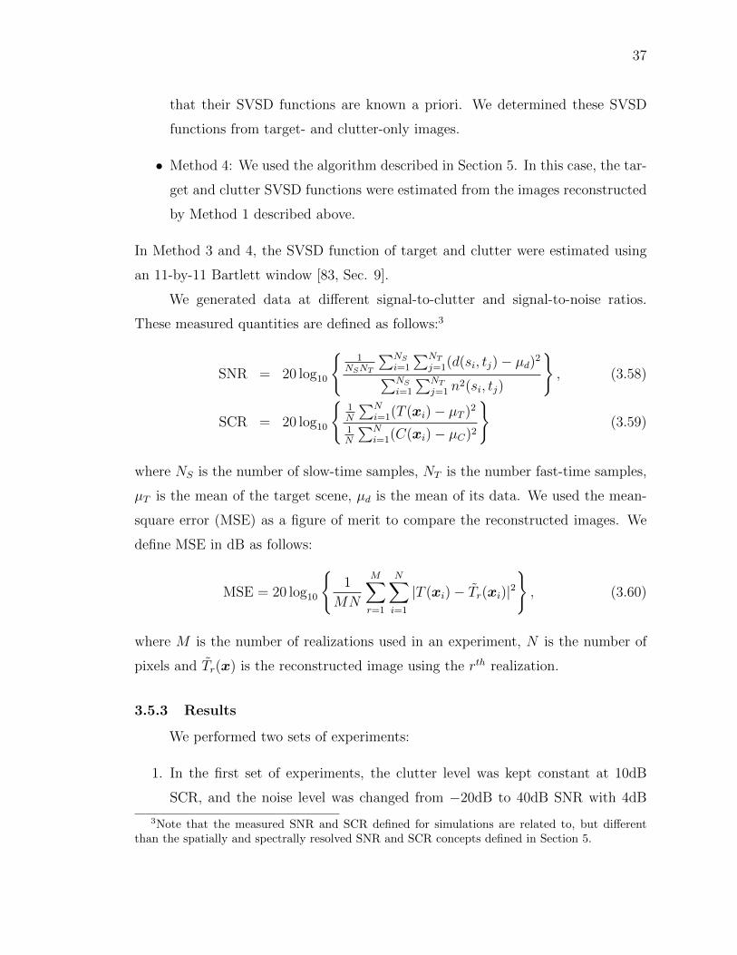
37
that their SVSD functions are known a priori. We determined these SVSD
functions from target- and clutter-only images.
• Method 4: We used the algorithm described in Section 5. In this case, the tar-
get and clutter SVSD functions were estimated from the images reconstructed
by Method 1 described above.
In Method 3 and 4, the SVSD function of target and clutter were estimated using
an 11-by-11 Bartlett window [83, Sec. 9].
We generated data at different signal-to-clutter and signal-to-noise ratios.
These measured quantities are defined as follows:3
SNR = 20 log10
1
NSNT
∑NSi=1
∑NTj=1(d(si, tj)− µd)2∑NS
i=1
∑NTj=1 n
2(si, tj)
, (3.58)
SCR = 20 log10
1N
∑Ni=1(T (xi)− µT )2
1N
∑Ni=1(C(xi)− µC)2
(3.59)
where NS is the number of slow-time samples, NT is the number fast-time samples,
µT is the mean of the target scene, µd is the mean of its data. We used the mean-
square error (MSE) as a figure of merit to compare the reconstructed images. We
define MSE in dB as follows:
MSE = 20 log10
1
MN
M∑r=1
N∑i=1
|T (xi)− Tr(xi)|2, (3.60)
where M is the number of realizations used in an experiment, N is the number of
pixels and Tr(x) is the reconstructed image using the rth realization.
3.5.3 Results
We performed two sets of experiments:
1. In the first set of experiments, the clutter level was kept constant at 10dB
SCR, and the noise level was changed from −20dB to 40dB SNR with 4dB
3Note that the measured SNR and SCR defined for simulations are related to, but differentthan the spatially and spectrally resolved SNR and SCR concepts defined in Section 5.

38
increments. Ten different realizations of noise were produced and added to
the clutter contaminated data simulated using (3.2).
2. In the second set of experiments, the noise level was kept constant at 10dB
SNR, and the clutter level was changed from −20dB to 40dB SCR with 4dB
increments. For each SCR level, ten different realizations of clutter were gen-
erated. The measurement data was simulated using (3.2).
We computed the MSE for each SNR and SCR level using the ten reconstructed
images, each one corresponding to a different noise or clutter realization. Figure 3.6
and Figure 3.10 show the MSE versus SNR and MSE verssus SCR performances of
the four methods described above. We see that for both sets of experiments Method
3 produces the lowest MSE values for all SNR and SCR levels. This is followed
by Method 4, Method 2 and Method 1. As SNR (or SCR) increases the difference
between the MSE values of Method 1 and Method 2 gets smaller as expected. We
also observed that as the SNR (or SCR) value increases, the difference between the
MSE values associated with Method 4 and Method 2 becomes larger. This can be
explained with better target SVSD estimation at higher SNR levels (or SCR) levels.
Figures 3.3 - 3.5 show the reconstructed images (averaged over ten realizations)
for SNR levels of −20, 8, 40dB and 10dB SCR. We see that at −20dB SNR, the
method described in [1] cannot recover the scene. At 10dB SNR, however, all four
methods can recover the scene, but Method 1 retains singularities induced by noise
and clutter and Method 3 produces visually the cleanest image.
Figure 3.7 - 3.9 show the reconstructed images for SCR levels of −20, 8, 40dB
and 10dB SNR. We see that all four methods recover a visually recognizable scene at
all SCR levels. However, at low SCR the clutter patches are visually more prominent
than the target in images produced by Method 1, 2 and 4. Only Method 3, which
uses SVSD function estimated from a clutter free scene, can suppress clutter and
recover target with good contrast. At high SCR levels, the target intensity dominates
and therefore all four methods can recover the target scene. Method 3 and 4 perform
better than Method 1 and 2 in suppressing the clutter strength.

39
10 20 30 40 50 60
10
20
30
40
50
60
0
0.1
0.2
0.3
0.4
0.5
0.6
0.7
0.8
0.9
1
(a)
20 40 60 80 100 120
20
40
60
80
100
120
140
160
180
0
5
10
15
20
25
30
(b)
Figure 3.1: (a) Target and (b) radar data, where horizontal and verticallines correspond to slow- and fast-time variables s and t respectively.
10 20 30 40 50 60
10
20
30
40
50
60
0
0.1
0.2
0.3
0.4
0.5
0.6
0.7
0.8
0.9
1
(a)
20 40 60 80 100 120
20
40
60
80
100
120
140
160
180 0
5
10
15
20
25
30
(b)
Figure 3.2: (a) Target embedded in clutter and (b) its radar data whenSCR is 10dB.
3.5.4 Numerical Simulations with Real Data
As a second set of simulations, we apply the Algorithm 1 to real data pro-
vided by Air Force Research Laboratories’ Wide Angle SAR experiment [2]. In this
experiment, radar data is collected by an X-band system over a parking lot that
includes 33 civilian vehicles. The average range to a target is 10km and the radar
data provided contains 14243 pulses with 47 frequency bins. Figures 3.11 (a)-(b)
show the SAR images reconstructed from wide-angle SAR data [2] by Method 1
and Method 4 for Chevrolet Impala (dataset PH fcara1 0216.mat). We observe

40
that there is strong clutter in the lower-left part of the image reconstructed by FBP.
However, this clutter is suppressed when we use the non-stationary reconstruction
algorithm.
3.6 Conclusion
In this chapter, we presented novel SAR inversion methods when the data is
noisy or clutter is present in the scene. First, we described a novel statistical model
for SAR target and clutter. We performed numerical simulations to demonstrate the
performance of the method both with synthetic and real data. These simulations also
included image reconstruction with three other methods to compare the performance
of the method. Numerical simulations show a reduction in the MSE of the images
as well as improved image quality compared to other SAR image reconstruction
methods.

41
10 20 30 40 50 60
10
20
30
40
50
60
0
0.1
0.2
0.3
0.4
0.5
0.6
0.7
0.8
0.9
1
(a)
10 20 30 40 50 60
10
20
30
40
50
60
0
0.1
0.2
0.3
0.4
0.5
0.6
0.7
0.8
0.9
1
(b)
10 20 30 40 50 60
10
20
30
40
50
60
0
0.1
0.2
0.3
0.4
0.5
0.6
0.7
0.8
0.9
1
(c)
10 20 30 40 50 60
10
20
30
40
50
60
0
0.1
0.2
0.3
0.4
0.5
0.6
0.7
0.8
0.9
1
(d)
Figure 3.3: Reconstructed images using (a) the method in [1], (b) withstationary target and clutter assumption, (c) non-stationary target andclutter assumption with known SVSD, (d) non-stationary target and clut-ter assumption with known SVSD when SNR is -20dB and SCR is 10dB.

42
10 20 30 40 50 60
10
20
30
40
50
60
0
0.1
0.2
0.3
0.4
0.5
0.6
0.7
0.8
0.9
1
(a)
10 20 30 40 50 60
10
20
30
40
50
60
0
0.1
0.2
0.3
0.4
0.5
0.6
0.7
0.8
0.9
1
(b)
10 20 30 40 50 60
10
20
30
40
50
60
0
0.1
0.2
0.3
0.4
0.5
0.6
0.7
0.8
0.9
1
(c)
10 20 30 40 50 60
10
20
30
40
50
60
0
0.1
0.2
0.3
0.4
0.5
0.6
0.7
0.8
0.9
1
(d)
Figure 3.4: Reconstructed images using (a) the method in [1], (b) withstationary target and clutter assumption, (c) non-stationary target andclutter assumption with known SVSD, (d) non-stationary target and clut-ter assumption with known SVSD when SNR is 8dB and SCR is 10dB.

43
10 20 30 40 50 60
10
20
30
40
50
60
0
0.1
0.2
0.3
0.4
0.5
0.6
0.7
0.8
0.9
1
(a)
10 20 30 40 50 60
10
20
30
40
50
60
0
0.1
0.2
0.3
0.4
0.5
0.6
0.7
0.8
0.9
1
(b)
10 20 30 40 50 60
10
20
30
40
50
60
0
0.1
0.2
0.3
0.4
0.5
0.6
0.7
0.8
0.9
1
(c)
10 20 30 40 50 60
10
20
30
40
50
60
0
0.1
0.2
0.3
0.4
0.5
0.6
0.7
0.8
0.9
1
(d)
Figure 3.5: Reconstructed images using (a) the method in [1], (b) withstationary target and clutter assumption, (c) non-stationary target andclutter assumption with known SVSD, (d) non-stationary target and clut-ter assumption with known SVSD when SNR is 40dB and SCR is 10dB.

44
−20 −10 0 10 20 30 40−70
−65
−60
−55
−50
−45
−40
−35
−30
−25
SNR (in dB)
MS
E (
in d
B)
FBPStationaryNon−stationary, known SVSDNon−stationary, unknown SVSD
Figure 3.6: MSE (vertical axis, in log scale) versus SNR (horizontal axis)averaged over ten reconstructed images for each SNR level using fourdifferent image reconstruction methods.

45
10 20 30 40 50 60
10
20
30
40
50
60
0
0.1
0.2
0.3
0.4
0.5
0.6
0.7
0.8
0.9
1
(a)
10 20 30 40 50 60
10
20
30
40
50
60
0
0.1
0.2
0.3
0.4
0.5
0.6
0.7
0.8
0.9
1
(b)
10 20 30 40 50 60
10
20
30
40
50
60
0
0.1
0.2
0.3
0.4
0.5
0.6
0.7
0.8
0.9
1
(c)
10 20 30 40 50 60
10
20
30
40
50
60
0
0.1
0.2
0.3
0.4
0.5
0.6
0.7
0.8
0.9
1
(d)
Figure 3.7: Reconstructed images using (a) the method in [1], (b) withstationary target and clutter assumption, (c) non-stationary target andclutter assumption with known SVSD, (d) non-stationary target and clut-ter assumption with known SVSD when SCR is -20dB and SNR is 10dB.

46
10 20 30 40 50 60
10
20
30
40
50
60
0
0.1
0.2
0.3
0.4
0.5
0.6
0.7
0.8
0.9
1
(a)
10 20 30 40 50 60
10
20
30
40
50
60
0
0.1
0.2
0.3
0.4
0.5
0.6
0.7
0.8
0.9
1
(b)
10 20 30 40 50 60
10
20
30
40
50
60
0
0.1
0.2
0.3
0.4
0.5
0.6
0.7
0.8
0.9
1
(c)
10 20 30 40 50 60
10
20
30
40
50
60
0
0.1
0.2
0.3
0.4
0.5
0.6
0.7
0.8
0.9
1
(d)
Figure 3.8: Reconstructed images using (a) the method in [1], (b) withstationary target and clutter assumption, (c) non-stationary target andclutter assumption with known SVSD, (d) non-stationary target and clut-ter assumption with known SVSD when SCR is 8dB and SNR is 10dB.

47
10 20 30 40 50 60
10
20
30
40
50
60
0
0.1
0.2
0.3
0.4
0.5
0.6
0.7
0.8
0.9
1
(a)
10 20 30 40 50 60
10
20
30
40
50
60
0
0.1
0.2
0.3
0.4
0.5
0.6
0.7
0.8
0.9
1
(b)
10 20 30 40 50 60
10
20
30
40
50
60
0
0.1
0.2
0.3
0.4
0.5
0.6
0.7
0.8
0.9
1
(c)
10 20 30 40 50 60
10
20
30
40
50
60
0
0.1
0.2
0.3
0.4
0.5
0.6
0.7
0.8
0.9
1
(d)
Figure 3.9: Reconstructed images using (a) the method in [1], (b) withstationary target and clutter assumption, (c) non-stationary target andclutter assumption with known SVSD, (d) non-stationary target and clut-ter assumption with known SVSD when SCR is 40dB and SNR is 10dB.

48
−20 −10 0 10 20 30 40−70
−65
−60
−55
−50
−45
−40
−35
−30
SCR (in dB)
MS
E (
in d
B)
FBPStationaryNon−stationary, known SVSDNon−stationary, unknown SVSD
Figure 3.10: MSE (vertical axis, in log scale) versus SCR (horizontalaxis) averaged over ten reconstructed images for each SCR level usingfour different image reconstruction methods.
(a) (b)
Figure 3.11: (a) Real SAR image reconstructed from wide-angle SARdata [2] by Method 1, (b) and Method 4.

CHAPTER 4
AN ANALYTIC SAR INVERSION METHOD BASED ON
BEST LINEAR UNBIASED ESTIMATION
In this chapter, we develop an analytic SAR inversion formula based on best lin-
ear unbiased estimation criterion. For a brief review of the best linear unbiased
estimation method, see Appendix F.
We assume that the clutter is a pseudo-stationary process and additive noise is
stationary in fast-time and uncorrelated in slow-time. We formulate the image for-
mation as a constrained optimization problem. We present an approximate solution
for the optimization problem using microlocal analysis, the methods of Lagrange
multipliers and variational derivatives. The resulting estimator is a composition of
two linear operators, one of which is a pseudo-differential operator and the other
one is an FIO in the form of a filtered-backprojection operator. The filters associ-
ated with these two operators are given in terms of the noise power spectral density
function, spatially-varying clutter spectral density function, as well as the Beylkin
determinant, antenna beam patterns, transmitted waveform and geometric spread-
ing factors. The inversion formula has the advantages of computational efficiency,
applicability to arbitrary imaging geometries and multiple SAR modalities.
4.1 Received Signal Model
4.1.1 Forward Model
Under the start-stop approximation, for many SAR modalities [1], [3], [16],
noise-free scattered field data, d, can be modeled as follows:
d(s, t) ≈ F [V ](s, t) :=
∫e−i2πω(t−R(s,x)/c)A(x, s, ω)V (x) dωdx, (4.1)
where s and t denote slow-time and fast-time, respectively, and V denotes the scene
reflectivity function. R denotes the range between the antenna(s) and the scatterer
49

50
located at x at slow-time s. For a bi-static configuration, R is given by
R(s,x) = |γT (s)− x|+ |γR(s)− x| (4.2)
where γT (s) and γR(s) denote the transmitter and the receiver trajectories, respec-
tively.
We assume that for some mA, the amplitude term A satisfies the symbol
estimate [1], [16]:
sup(s,x)∈K
| ∂αω∂βs ∂ρxA(x, s, ω) | ≤ BK,α,β,ρ (1 + |ω|)mA−|α| (4.3)
where K is any compact subset of R×R2, BK,α,β,ρ is a K,α, β,ρ dependent constant,
and ρ is a multi-index. Under the assumption in (4.3), F becomes a Fourier integral
operator [43]–[46]. For the rest of this chapter, we refer to F as the forward operator.
Let T (x), x ∈ ΩT ⊆ R2 denote the target scene. We assume that the target
is embedded in clutter and write
V (x) = T (x) + C(x). (4.4)
Taking into account the additive thermal noise we model the received signal
as
d(s, t) = F [V ](s, t) + n(s, t) = F [T + C](s, t) + n(s, t). (4.5)
4.1.2 Target, Clutter and Noise Models
Unlike the target models in Chapters 3 and 6, in this chapter, we model target
as a deterministic quantity.
We model clutter, C(x), x ∈ ΩC ⊆ R2, as a zero-mean, pseudo-stationary
process with the following spectral representation:
C(x) =
∫e−i2π(x−x′)·ζSC(x, ζ) dζdB(x′) (4.6)
where B(x′) is the Wiener process and SC(x, ζ) satisfies the following symbol esti-

51
mate
supx∈U| ∂αζ ∂βxSC(x, ζ) | ≤ BC
U,α,β(1 + |ζ|)mC−|α| (4.7)
where U is any compact subset of R2, BTU,α,β is a constant that depends on the
multi-indices α,β, and U , mC are real numbers.
The autocovariance function of C is given by
E[C(x)C(x)
]=
∫ei2π(x−x)·ζSC(x, ζ)SC(x, ζ) dζ. (4.8)
We assume that the additive measurement noise is a zero-mean, stationary
process in fast-time and statistically mutually uncorrelated in slow-time and write
Sn(s, ω) = σ(s)Sn(ω). (4.9)
The autocovariance function of the noise is given by
E[n(s, t)n(s′, t′)] = σ2(s)δ(s− s′)Rn(t, t′) (4.10)
where
Rn(t, t′) =
∫ei2πω(t−t′)|Sn(ω)|2 dω (4.11)
and |Sn(s, ω)|2 is the power spectral density function of the noise. To avoid peculiar
behavior, we assume Sn satisfies the following condition
E[|n(s, t)|2] = σ2(s)
∫ ∣∣∣Sn(ω)∣∣∣2 dω < +∞. (4.12)
Finally, without loss of generality, we assume that the clutter and noise are
mutually statistically uncorrelated.

52
4.2 Image Formation based on BLUE Criterion
4.2.1 Problem Statement
Let Kbl be a linear operator and
Tbl(z) = Kbl[d](z) (4.13)
be an image of the target. We wish to design Kbl so that the following conditions
are satisfied:
1. Kbl is a composition of two FIOs, i.e., Kbl = K2blK1
bl. Specifically, K1bl is the
following filtered-backprojection (FBP) operator:
T (x′) = K1bl[d](x′) :=
∫ei2πω(t−R(s,x′)/c)Q1
bl(x′, s, ω)d(s, t) dωdsdt (4.14)
where Q1bl satisfies a symbol estimate similar to the one stated in (4.3).
K2bl is a pseudo-differential operator with the following kernel:
Q2bl(z,x
′) =
∫ei2π(x′−z)·ζQ2
bl(z, ζ)dζ (4.15)
where Q2bl satisfies a symbol estimate similar to the one stated in (4.3). Note
that Q1bl is a filter applied prior to the backprojection and Q2
bl is a filter applied
after the backprojection operation.
2. Tbl(z) = Kbl[d](z) is an unbiased estimate of T (x), x ∈ ΩT ⊆ R2 up to the
leading-order term of Kbl.4
3. The total variance of the estimate∫E[|Tbl(z)− E[Tbl(z)]|2
]dz (4.16)
is minimum among all the linear estimates satisfying Condition 1 and 2 above.
4Here the “leading-order” is in the microlocal sense [43]–[46], meaning that the higher orderterms are smoother than the leading-order one. In other words, the bias of the estimate is onedegree smoother than E[Tbl].

53
We refer to Tbl(z) = Kbl[d](z) satisfying Conditions 1-3 as the best linear
unbiased estimate (BLUE) of T (z) and Kbl as the BLUE operator. Note that we
require the estimator to be not only linear, unbiased and minimum variance, but
also of a particular form as stated in Condition 1.
Clearly, determining the BLUE operator is equivalent to determining the filters
Q1bl and Q2
bl satisfying Conditions 1-3.
4.2.2 The Bias and Total Variance of BLUE
We begin by defining a bias image
B(z) = E[Tbl(z)]− IΩ[T ](z) (4.17)
where
IΩ[T ](z) :=
∫Ωz
χΩ(z, ξ)ei2π(x−z)·ξT (x) dξdx (4.18)
and χΩ(z, ξ) is a smoothed version of the characteristic function of Ω given by
Ω = ∪zΩz with
Ωz =ξ : ξ =
ω
c∇xR(s,x) |x=z, A(z, s, ω) 6= 0
. (4.19)
The image IΩ[T ] is the best image (in the least square sense) we can obtain given
the bandwidth of the transmitted waveform and the effective length of the synthetic
aperture. Ω can be viewed as the set of target Fourier coefficients that can be
obtained from our measurements.
Let
CTbl(z, z′) := E[(Tbl(z)− E[Tbl(z)])(Tbl(z′)− E[Tbl(z′)])
](4.20)

54
denote the autocorrelation function of Tbl(z). We next define
J Cbl (Q1
bl, Q2bl) =
∫E[|KblF [C](z)|2]dz, (4.21)
J nbl (Q
1bl, Q
2bl) =
∫E[|Kbl[n](z)|2]dz. (4.22)
Lemma 2: We assume that the image Tbl is formed by the BLUE operator as
outlined in Conditions 1-3, where the filters Q1bl and Q2
bl satisfy the symbol estimates
similar to the one stated in (4.7) and where the data d are given by (4.5). We
assume that the geometrical conditions on the flight trajectories and the antenna
beam patterns satisfy certain conditions such that artifacts are avoided [82].
(i) Then, the leading-order singularities of the bias image are
B(z) ≈∫
ei2π(x−z)·ξ(Q2bl(z, ξ)Q1
bl(z, ξ)A(x, ξ)η(x, z, ξ)− χΩ(z,ξ)
)dξdx.
(4.23)
(ii) The total variance of the BLUE image is given by∫CTbl(z, z)dz ≈ J C
bl (Q1bl, Q
2bl) + J C
bl (Q1bl, Q
2bl) (4.24)
where the leading-order singularities of each term in (4.24) are
J Cbl (Q1
bl, Q2bl) ≈
∫|Q2
bl(x, ξ)Q1bl(x, ξ)A(x, ξ)η(x,x, ξ)|2|SC(x, ξ)|2 dξdx
(4.25)
and
J nbl (Q
1bl, Q
2bl) ≈
∫|Q2
bl(x, ξ)Q1bl(x, ξ)|2η(x,x, ξ)|Sn(ξ)|2dxdξ. (4.26)
Proof:

55
(i) Let
T 1bl(z) := K1
blF [T ](z). (4.27)
We simplify K1blF as in [1]. Using (4.1) in (4.14) and carrying out the t
integration and one of the ω integrations results in
K1blF [T ](x′) :=
∫ei2π 2ω
c(R(s,x)−R(s,x′))Q1
bl(x′, s, ω)A(x, s, ω)T (x)dωdsdx
(4.28)
Next, we use the identity
h(x)− h(x′) = (x− x′) ·∫ 1
0
∇h(x′ + λ(x− x′))dλ. (4.29)
For h(x) = 2ωcR(s,x) we write
2ω
c(R(s,x)−R(s,x′)) =
ω
c(x− x′) ·Ξ(s,x,x′), (4.30)
where for x = x′ we can write
Ξ(s,x′,x′) = ∇h(x′) = L(x′, s) ·Dψ(x′), (4.31)
and Dψ(x′) is given by
Dψ(x′) =
1 0 ∇x′1ψ(x′)
0 1 ∇x′2ψ(x′)
(4.32)
and
L(x′, s) =γT (s)− x′
|γT (s)− x′|+γR(s)− x′
|γR(s)− x′|(4.33)

56
is the bi-static antenna look direction. We make the change of variables
(s, ω)→ ξ =2ω
cΞ(s,x,x′) (4.34)
where the geometrical assumptions made for the trajectory makes the change
of variables non-singular [82]. Then, (4.28) can be written as
K1blF [T ](x′) ≈
∫ei2π(x−x′)·ξQ1
bl(x′, ξ)A(x, ξ)η(x,x′, ξ)T (x)dxdξ (4.35)
where
η(x,x′, ξ) =
∣∣∣∣∂(s, ω)
∂ξ
∣∣∣∣ (4.36)
is the determinant of the Jacobian coming from the change of variables.
Combining (4.35) with K2bl we obtain
KblF [T ](z) =
∫Q2bl(z, ζ)ei2π[(x−x′)·ξ+(x′−z)·ζ]Q1
bl(x′, ξ)
× A(x, ξ)η(x,x′, ξ)T (x)dξdxdx′dζ. (4.37)
We next apply the method of the stationary phase in the variables x′ and ζ
simultaneously for the phase function:5
φ1(x,x′, z, ζ, ξ) = (x′ − z) · ζ + (x− x′) · ξ. (4.38)
The method of the stationary phase results in the critical points at
∇x′φ1 → ζ = ξ, (4.39)
∇ζφ1 → x′ = z. (4.40)
5 The determinant of the Hessian of φ1 is −1. See Appendix G.1 for the computation of theHessian of φ1.

57
The leading-order term of (4.37) is then
KblF [T ](z) ≈∫
ei2π(x−z)·ξQ2bl(z, ξ)Q1
bl(z, ξ)A(x, ξ)η(x, z, ξ)T (x)dξdx.
(4.41)
Combining (4.41) and (4.18), the leading-order singularities of the bias image
is given by
B(z) =E[Tbl(z)]− IΩ[T ](z) (4.42)
≈∫
ei2π(x−z)·ξ(Q2bl(z, ξ)Q1
bl(z, ξ)A(x, ξ)η(x, z, ξ)− χΩ(z, ξ))
× T (x)dξdx. (4.43)
(ii) The total variance of the BLUE image is given by:∫CTbl(z, z)dz =
∫E[|(Tbl(z)− E[Tbl(z)|2])
]dz, (4.44)
=
∫E[|KblF [T + C](z) +Kbl[n](z)− T (z)|2
]dz. (4.45)
Using the facts that Tbl is unbiased up to its leading-order singularities, the
noise and clutter are statistically uncorrelated, and the approximation in
(4.37), we get∫CTbl(z, z)dz ≈
∫ (E[|KblF [C](z)|2] + E[|Kbl[n](z)|2]
)dz. (4.46)
Using the approximation to Kbl given in (4.41), J Cbl can be expressed as
J Cbl (Q1
bl, Q2bl) =
∫E[(KblF [C](z))(KblF [C](z))
]dz,
≈∫
ei2π(x−z)·ξQ2bl(z, ξ)Q1
bl(z, ξ)A(x, ξ)η(x, z, ξ)
× e−i2π(x−z)·ξQ2bl(z, ξ)Q1
bl(z, ξ)A(x, ξ)η(x, z, ξ)
× E[C(x)C(x)]dxdξdxdξdz. (4.47)

58
The phase function of the integrand in (4.47) is given by
φ2(x, ξ, x, ξ, z) = (x− z) · ξ − (x− z) · ξ. (4.48)
to approximate z and ξ integrations, we apply the method of the stationary
phase in the variables z and ξ, simultaneously.6 We obtain the critical points
at
∇zφ2 → ξ = ξ, (4.49)
∇ξφ2 → z = x. (4.50)
Hence, the leading-order term of (4.47) is
J Cbl (Q1
bl, Q2bl) ≈
∫ei2π(x−x)·ξ|Q2
bl(x, ξ)Q1bl(x, ξ)|2A(x, ξ)η(x, x, ξ)
× A(x, ξ)η(x, x, ξ)E[C(x)C(x)]dxdξdx. (4.51)
Inserting (4.8) in (4.51), we obtain
J Cbl (Q1
bl, Q2bl) ≈
∫ei2π(x−x)·ξ|Q2
bl(x, ξ)Q1bl(x, ξ)|2A(x, ξ)η(x, x, ξ)
× A(x, ξ)η(x, x, ξ)e−i2π(x−x)·ζSC(x, ζ)SC(x, ζ) dζdxdξdx.
(4.52)
We apply the method of the stationary phase to the phase function one more
time in variables x and ζ, simultaneously:7
φ3(x, x, ξ, ζ) = (x− x) · ξ − (x− x) · ζ (4.53)
6The determinant of the Hessian of φ2 is −1. See Appendix G.2 for the computation of theHessian of φ2.
7The determinant of the Hessian of φ3 is −1. See Appendix G.3 for the computation of theHessian of φ3.

59
which results in the critical conditions
∇xφ3 → ζ = ξ, (4.54)
∇ζφ3 → x = x. (4.55)
Hence, the leading-order term of (4.52) is
J Cbl (Q1
bl, Q2bl) ≈
∫|Q2
bl(x, ξ)Q1bl(x, ξ)A(x, ξ)η(x,x, ξ)|2|SC(x, ξ)|2 dξdx.
(4.56)
Following steps similar to those in (4.47)-(4.52) and using (4.11), it can be
shown that the leading-order term of J nbl is
J nbl (Q
1bl, Q
2bl) ≈
∫|Q2
bl(x, ξ)Q1bl(x, ξ)|2η(x,x, ξ)|Sn(ξ)|2dxdξ. (4.57)
4.2.3 Derivation of the Imaging Filters
The leading-order singularities of the bias image is given by
B(z) ≈∫
ei2π(x−z)·ξ(Q2bl(z, ξ)Q1
bl(z, ξ)A(x, ξ)η(x, z, ξ)− χΩ(z, ξ))T (x)dξdx.
(4.58)
The leading-order contribution to (4.58) occurs when x = z. Let
B(Q1bl, Q
1bl) := Q2
bl(z, ξ)Q1bl(z, ξ)A(z, ξ)η(z, z, ξ)− χΩ(z, ξ). (4.59)
For the leading-order singularities of Tbl to be unbiased, the following must
hold
B(Q1bl, Q
2bl) = 0 (4.60)
for all z ∈ ΩT . Our objective is to design the filters Q1bl and Q2
bl so that the leading-

60
order singularities of the total variance∫CTbl(z, z)dz ≈
∫ (E[|KblF [C](z)|2] + E[|Kbl[n](z)|2]
)dz (4.61)
is minimized subject to the constraint in (4.60).
We use the method of Lagrange multipliers to address this constrained op-
timization problem. Let λ(z, ξ) be the Lagrange multiplier associated with the
constraint B(Q1bl, Q
2bl) = 0. Recall that∫CTbl(z, z)dz ≈ J C
bl (Q1bl, Q
2bl) + J n
bl (Q1bl, Q
2bl) (4.62)
where
J Cbl (Q1
bl, Q2bl) =
∫E[|KblF [C](z)|2]dz, (4.63)
J nbl (Q
1bl, Q
2bl) =
∫E[|Kbl[n](z)|2]dz. (4.64)
To incorporate the constraint (4.60) into the minimization, we define
J λbl (Q
1bl, Q
2bl, λ) :=
∫λ(z, ξ)B(Q1
bl, Q2bl)dzdξ. (4.65)
We next define the following objective functional:
Jbl(Q1bl, Q
2bl, λ) = J C
bl (Q1bl, Q
2bl) + J n
bl (Q1bl, Q
2bl)− J λ
bl (Q1bl, Q
2bl, λ). (4.66)
Theorem 2: Let the data d be given by (4.5) and Tbl be given by (4.13). If the
filters Q1bl and Q2
bl in (4.14) and (4.15) are chosen as
Q1bl(x
′, ξ) =A(x′, ξ)η(x′,x′, ξ)χΩ(x′, ξ)
|A(x′, ξ)η(x′,x′, ξ)|2|SC(x′, ξ)|2 + η(x′,x′, ξ)|Sn(ξ)|2(4.67)
and
Q2bl(z,x
′) =
∫ei2π(x′−z)·ξ |A(z, ξ)η(z, z, ξ)|2|SC(z, ξ)|2 + η(z, z, ξ)|Sn(ξ)|2
|A(z, ξ)η(z, z, ξ)|2dξ.
(4.68)

61
where χΩ(x′, ξ) is a smooth function that prevents division by 0 and η(x′,x′, ξ),
SC(z, ξ) and Sn(ξ) are as defined in (4.36), (4.6), (4.9), respectively. Then, the
followings hold:
(i) The leading-order singularities of E[Tbl(z)] is equal to the leading order singu-
larities of T (z).8
(ii) CTbl(z, z) is minimized at its leading-order singularities.
(iii) With these choice of filters, the variance of Tbl at its leading-order singularities
is given by
CTbl(z, z) ≈∫|A(z, ξ)η(z, z, ξ)|2|SC(z, ξ)|2 + η(z, z, ξ)|Sn(ξ)|2
|A(z, ξ)η(z, z, ξ)|2dξ. (4.69)
Proof: Our objective is to determine Q1bl, Q
2bl, λ that minimizes the following
objective functional:
Jbl(Q1bl, Q
2bl, λ) = J C
bl (Q1bl, Q
2bl) + J n
bl (Q1bl, Q
2bl)− J λ
bl (Q1bl, Q
2bl, λ). (4.70)
(i)-(ii) Having obtained approximations to each functional in (4.70), we study the
variational derivative of (4.70) with respect to Q2bl, Q
1bl and λ. We evaluate
the variational derivative with respect to Q2bl as follows:
d
dεJ Cbl (Q2
bl + εQε)
∣∣∣∣ε=0
+d
dεJ nbl (Q
2bl + εQε)
∣∣∣∣ε=0
− d
dεJ λbl (Q
2bl + εQε)
∣∣∣∣ε=0
= 0
(4.71)
which is given by
0 = 2 Re
∫Qε(x, ξ)
Q2bl(x, ξ)|Q1
bl(x, ξ)|2
× (|A(x, ξ)η(x,x, ξ)|2|SC(x, ξ)|2 + η(x,x, ξ)|Sn(ξ)|2)
dξdx
−∫λ(x, ξ)Qε(x, ξ)Q1
bl(x, ξ)A(x, ξ)η(x,x, ξ)dξdx. (4.72)
8The bias image B(z) is one degree smoother than the E[Tbl(z)].

62
We rewrite (4.72) as follows:
0 = 2 Re
∫Qε
(Q2bl|Q
1bl|2(|Aη|2|SC |2 + η|Sn|2)− 1
2λQ1
blAη
)dxdξ
+ Im
∫QελQ
1blAηdxdξ. (4.73)
(4.73) must hold for all Qε including real-valued Qε. Hence, we obtain the
following two relations on the filter Q1bl:
Q2bl|Q
1bl|2(|Aη|2|SC |2 + η|Sn|2)− 1
2λQ1
blAη = 0 (4.74)
and
Im λQ1blAη = 0. (4.75)
The variational derivative with respect to Q1bl provides an equation equivalent
to (4.73). Therefore, we only use the variational derivative with respect to Q2bl
and λ to determine the BLUE filters Q1bl and Q2
bl. Finally, we evaluate the
variational derivative of Jbl or J λbl with respect to λ and set it equal to 0 as
follows:
d
dεJ λbl (Q
1bl, Q
2bl, λ+ ελε)
∣∣∣∣ε=0
≈∫λε(x, ξ)
(Q2bl(x, ξ)Q1
bl(x, ξ)A(x, ξ)η(x,x, ξ)− χΩ(x, ξ))
dξdx = 0.
(4.76)
Since (4.76) must be true for all λε, we obtain
Q2bl(x, ξ)Q1
bl(x, ξ)A(x, ξ)η(x,x, ξ) = χΩ(x, ξ) (4.77)
where χΩ(x, ξ) is a smooth function that prevents division by 0. Using (4.77)

63
in (4.74), we obtain
λ(x, ξ) = 2|A(x, ξ)η(x,x, ξ)|2|SC(x, ξ)|2 + η(x,x, ξ)|Sn(ξ)|2
|A(x, ξ)η(x,x, ξ)|2. (4.78)
To satisfy the condition in (4.75), we choose the filter Q1bl
Q1bl(x
′, ξ) =A(x′, ξ)η(x′,x′, ξ)χΩ(x′, ξ)
|A(x′, ξ)η(x′,x′, ξ)|2|SC(x′, ξ)|2 + η(x′,x′, ξ)|Sn(ξ)|2, (4.79)
and from (4.77) we evaluate Q2bl
Q2bl(z,x
′) =
∫ei2π(x′−z)·ξ |A(z, ξ)η(z, z, ξ)|2|SC(z, ξ)|2 + η(z, z, ξ)|Sn(ξ)|2
|A(z, ξ)η(z, z, ξ)|2dξ.
(4.80)
(iii) Recall from (4.61) that the variance of the estimator is given by
CTbl(z, z) ≈E[|KblF [C](z)|2] + E[|Kbl[n](z)|2]. (4.81)
Inserting the approximations to E[|KblF [C](z)|2] and E[|Kbl[n](z)|2], we get
CTbl(z, z) ≈∫ (|A(z, ξ)η(z, z, ξ)|2|SC(z, ξ)|2 + η(z, z, ξ)|Sn(ξ)|2
)× |Q2
bl(z, ξ)Q1bl(z, ξ)|2dξ. (4.82)
Inserting the expression forQ1blQ
2bl in (4.77) into (4.82), we obtain the minimum
variance
CTbl(z, z) ≈∫|A(z, ξ)η(z, z, ξ)|2|SC(z, ξ)|2 + η(z, z, ξ)|Sn(ξ)|2
|A(z, ξ)η(z, z, ξ)|2dξ. (4.83)

64
4.3 Numerical Simulations
We consider a scene with an airplane-like object in the center as the target.
The object has various intensity levels to show that the algorithm reconstructs the
target scene with correct intensities at correct locations.
A scene of 100 m×100 m is discretized into 64×64 pixels. A bi-static antenna
system with π/18 separation between the transmitter and receiver, flies over the
scene on a circular trajectory γ(s) = [11 cos s, 11 sin s, 6.5] km uniformly sampled for
s ∈ [0, 2π] at 128 points. It is assumed that A(x, ω, s) = 1, which corresponds to an
isotropic antenna radiating a delta-like impulse and pre-compensation of geometric
spreading factors in the FBP data.
Gaussian noise is added to the projection data to simulate the additive thermal
noise. The clutter model described in Section 3.5 with the mask shown in Figure 3.2
is used here as well. The images are reconstructed via deterministic FBP, statistical
FBP with stationary target and clutter models; and BLUE criterion at various SNR
and SCR levels. For this set of simulations, the BLUE reconstruction method is
applied under the stationary clutter assumption, hence we drop the x dependence on
the spectral density function in filter (4.67). The target and clutter spectral densities
are provided a priori to the reconstruct images under stationarity assumption. The
reconstructed images are shown in Figures 4.1-4.10.
We performed ten sets of experiments. Figures 4.1-4.5 show the averages of
the ten reconstructed images using (a) deterministic FBP, (b) statistical FBP under
stationarity assumption, (c) BLUE after applying filter Q1bl, (d) BLUE after applying
filter Q2bl. We kept SCR constant at 10dB and increased SNR from 0dB to 30dB.
Similarly, Figures 4.6-4.10 show the average of the ten reconstructed images using
the same reconstruction methods at before. The SNR is kept constant at 10dB and
SCR is increased from 0dB to 32dB with 8 dB increments.
The plots in Figure 4.11(a) show the MSE in log scale versus SNR (horizontal
axis) at a 10dB SNR and at 5 different SNR levels. The plots in Figure 4.11(b) show
the MSE versus SCR (horizontal axis) at a constant SNR level of 10dB averaged over
ten reconstructed images. It can be observed from these plots that the performance
of the BLUE method is almost as good as the stationary reconstruction method

65
even though the stationary reconstruction method requires both target and clutter
spectral density functions whereas BLUE method only requires the spectral density
function of the clutter.
The performances of these methods are similar when the SNR is constant
and SCR is changed since the filter (4.67) used in the reconstruction with BLUE
includes the spectral density function of the clutter. As compared to the determin-
istic FBP reconstruction there is an average of 15% improvement in the MSE of
the reconstructed images when the BLUE method is used. At high SNR levels, the
deterministic FBP method works well. Therefore, the performances of the deter-
ministic FBP and the BLUE are similar at 32dB SNR as shown in Figure 4.11(a).
4.4 Conclusion
In this chapter, we developed a novel analytic inversion method based on the
best linear unbiased estimation criterion where target is embedded in clutter and
received signal data is corrupted by thermal noise. The BLUE-based method only
requires the first and second statistics of the unknown, spectral density of the clutter
which can be estimated from the data by using the method described in the previous
chapter. The filter successfully suppresses the effect of noise and clutter.

66
10 20 30 40 50 60
10
20
30
40
50
60
0
0.1
0.2
0.3
0.4
0.5
0.6
0.7
0.8
0.9
1
(a)
10 20 30 40 50 60
10
20
30
40
50
60
0
0.1
0.2
0.3
0.4
0.5
0.6
0.7
0.8
0.9
1
(b)
10 20 30 40 50 60
10
20
30
40
50
60
0
0.1
0.2
0.3
0.4
0.5
0.6
0.7
0.8
0.9
1
(c)
10 20 30 40 50 60
10
20
30
40
50
60
0
0.1
0.2
0.3
0.4
0.5
0.6
0.7
0.8
0.9
1
(d)
Figure 4.1: The reconstructed images averaged over 10 realizations using(a) the deterministic FBP, (b) MMSE FBP, (c) BLUE after applyingfilter Q1, (d) BLUE after applying filter Q2. The SNR is 10dB and SCRis 0 dB.

67
10 20 30 40 50 60
10
20
30
40
50
60
0
0.1
0.2
0.3
0.4
0.5
0.6
0.7
0.8
0.9
1
(a)
10 20 30 40 50 60
10
20
30
40
50
60
0
0.1
0.2
0.3
0.4
0.5
0.6
0.7
0.8
0.9
1
(b)
10 20 30 40 50 60
10
20
30
40
50
60
0
0.1
0.2
0.3
0.4
0.5
0.6
0.7
0.8
0.9
1
(c)
10 20 30 40 50 60
10
20
30
40
50
60
0
0.1
0.2
0.3
0.4
0.5
0.6
0.7
0.8
0.9
1
(d)
Figure 4.2: The reconstructed images averaged over 10 realizations using(a) the deterministic FBP, (b) MMSE FBP, (c) BLUE after applyingfilter Q1, (d) BLUE after applying filter Q2. The SNR is 10dB and SCRis 8 dB.

68
10 20 30 40 50 60
10
20
30
40
50
60
0
0.1
0.2
0.3
0.4
0.5
0.6
0.7
0.8
0.9
1
(a)
10 20 30 40 50 60
10
20
30
40
50
60
0
0.1
0.2
0.3
0.4
0.5
0.6
0.7
0.8
0.9
1
(b)
10 20 30 40 50 60
10
20
30
40
50
60
0
0.1
0.2
0.3
0.4
0.5
0.6
0.7
0.8
0.9
1
(c)
10 20 30 40 50 60
10
20
30
40
50
60
0
0.1
0.2
0.3
0.4
0.5
0.6
0.7
0.8
0.9
1
(d)
Figure 4.3: The reconstructed images averaged over 10 realizations using(a) the deterministic FBP, (b) MMSE FBP, (c) BLUE after applyingfilter Q1, (d) BLUE after applying filter Q2. The SNR is 10dB and SCRis 16 dB.

69
10 20 30 40 50 60
10
20
30
40
50
60
0
0.1
0.2
0.3
0.4
0.5
0.6
0.7
0.8
0.9
1
(a)
10 20 30 40 50 60
10
20
30
40
50
60
0
0.1
0.2
0.3
0.4
0.5
0.6
0.7
0.8
0.9
1
(b)
10 20 30 40 50 60
10
20
30
40
50
60
0
0.1
0.2
0.3
0.4
0.5
0.6
0.7
0.8
0.9
1
(c)
10 20 30 40 50 60
10
20
30
40
50
60
0
0.1
0.2
0.3
0.4
0.5
0.6
0.7
0.8
0.9
1
(d)
Figure 4.4: The reconstructed images averaged over 10 realizations using(a) the deterministic FBP, (b) MMSE FBP, (c) BLUE after applyingfilter Q1, (d) BLUE after applying filter Q2. The SNR is 10dB and SCRis 24 dB.

70
10 20 30 40 50 60
10
20
30
40
50
60
0
0.1
0.2
0.3
0.4
0.5
0.6
0.7
0.8
0.9
1
(a)
10 20 30 40 50 60
10
20
30
40
50
60
0
0.1
0.2
0.3
0.4
0.5
0.6
0.7
0.8
0.9
1
(b)
10 20 30 40 50 60
10
20
30
40
50
60
0
0.1
0.2
0.3
0.4
0.5
0.6
0.7
0.8
0.9
1
(c)
10 20 30 40 50 60
10
20
30
40
50
60
0
0.1
0.2
0.3
0.4
0.5
0.6
0.7
0.8
0.9
1
(d)
Figure 4.5: The reconstructed images averaged over 10 realizations using(a) the deterministic FBP, (b) MMSE FBP, (c) BLUE after applyingfilter Q1, (d) BLUE after applying filter Q2. The SNR is 10dB and SCRis 32 dB.

71
10 20 30 40 50 60
10
20
30
40
50
60
0
0.1
0.2
0.3
0.4
0.5
0.6
0.7
0.8
0.9
1
(a)
10 20 30 40 50 60
10
20
30
40
50
60
0
0.1
0.2
0.3
0.4
0.5
0.6
0.7
0.8
0.9
1
(b)
10 20 30 40 50 60
10
20
30
40
50
60
0
0.1
0.2
0.3
0.4
0.5
0.6
0.7
0.8
0.9
1
(c)
10 20 30 40 50 60
10
20
30
40
50
60
0
0.1
0.2
0.3
0.4
0.5
0.6
0.7
0.8
0.9
1
(d)
Figure 4.6: The reconstructed images averaged over 10 realizations using(a) the deterministic FBP, (b) MMSE FBP, (c) BLUE after applyingfilter Q1, (d) BLUE after applying filter Q2. The SCR is 10dB and SNRis 0 dB.

72
10 20 30 40 50 60
10
20
30
40
50
60
0
0.1
0.2
0.3
0.4
0.5
0.6
0.7
0.8
0.9
1
(a)
10 20 30 40 50 60
10
20
30
40
50
60
0
0.1
0.2
0.3
0.4
0.5
0.6
0.7
0.8
0.9
1
(b)
10 20 30 40 50 60
10
20
30
40
50
60
0
0.1
0.2
0.3
0.4
0.5
0.6
0.7
0.8
0.9
1
(c)
10 20 30 40 50 60
10
20
30
40
50
60
0
0.1
0.2
0.3
0.4
0.5
0.6
0.7
0.8
0.9
1
(d)
Figure 4.7: The reconstructed images averaged over 10 realizations using(a) the deterministic FBP, (b) MMSE FBP, (c) BLUE after applyingfilter Q1, (d) BLUE after applying filter Q2. The SCR is 10dB and SNRis 8 dB.

73
10 20 30 40 50 60
10
20
30
40
50
60
0
0.1
0.2
0.3
0.4
0.5
0.6
0.7
0.8
0.9
1
(a)
10 20 30 40 50 60
10
20
30
40
50
60
0
0.1
0.2
0.3
0.4
0.5
0.6
0.7
0.8
0.9
1
(b)
10 20 30 40 50 60
10
20
30
40
50
60
0
0.1
0.2
0.3
0.4
0.5
0.6
0.7
0.8
0.9
1
(c)
10 20 30 40 50 60
10
20
30
40
50
60
0
0.1
0.2
0.3
0.4
0.5
0.6
0.7
0.8
0.9
1
(d)
Figure 4.8: The reconstructed images averaged over 10 realizations using(a) the deterministic FBP, (b) MMSE FBP, (c) BLUE after applyingfilter Q1, (d) BLUE after applying filter Q2. The SCR is 10dB and SNRis 16 dB.

74
10 20 30 40 50 60
10
20
30
40
50
60
0
0.1
0.2
0.3
0.4
0.5
0.6
0.7
0.8
0.9
1
(a)
10 20 30 40 50 60
10
20
30
40
50
60
0
0.1
0.2
0.3
0.4
0.5
0.6
0.7
0.8
0.9
1
(b)
10 20 30 40 50 60
10
20
30
40
50
60
0
0.1
0.2
0.3
0.4
0.5
0.6
0.7
0.8
0.9
1
(c)
10 20 30 40 50 60
10
20
30
40
50
60
0
0.1
0.2
0.3
0.4
0.5
0.6
0.7
0.8
0.9
1
(d)
Figure 4.9: The reconstructed images averaged over 10 realizations using(a) the deterministic FBP, (b) MMSE FBP, (c) BLUE after applyingfilter Q1, (d) BLUE after applying filter Q2. The SCR is 10dB and SNRis 24 dB.

75
10 20 30 40 50 60
10
20
30
40
50
60
0
0.1
0.2
0.3
0.4
0.5
0.6
0.7
0.8
0.9
1
(a)
10 20 30 40 50 60
10
20
30
40
50
60
0
0.1
0.2
0.3
0.4
0.5
0.6
0.7
0.8
0.9
1
(b)
10 20 30 40 50 60
10
20
30
40
50
60
0
0.1
0.2
0.3
0.4
0.5
0.6
0.7
0.8
0.9
1
(c)
10 20 30 40 50 60
10
20
30
40
50
60
0
0.1
0.2
0.3
0.4
0.5
0.6
0.7
0.8
0.9
1
(d)
Figure 4.10: The reconstructed images averaged over 10 realizations using(a) the deterministic FBP, (b) MMSE FBP, (c) BLUE after applying filterQ1, (d) BLUE after applying filter Q2. The SCR is 10dB and SNR is 32dB.

76
0 5 10 15 20 25 30 35−48
−46
−44
−42
−40
−38
−36
−34
−32
SNR (in dB)
MS
E (
in d
B)
FBPStationaryBLUE with Q
1
BLUE with Q1 and Q
2
(a)
0 5 10 15 20 25 30 35−44
−43
−42
−41
−40
−39
−38
−37
−36
−35
SCR (in dB)
MS
E (
in d
B)
FBPStationaryBLUE with Q
1
BLUE with Q1 and Q
2
(b)
Figure 4.11: MSE (vertical axis, in dB) versus (a) SNR (horizontalaxis) with constant SCR level at 10dB and (b) SCR (horizontal axis)with constant SNR level at 10dB averaged over ten reconstructed imagesusing four different image reconstruction methods.

PART II
77

CHAPTER 5
FBP-TYPE DIRECT EDGE ENHANCEMENT OF
SYNTHETIC APERTURE RADAR IMAGES
In this chapter, we consider a synthetic aperture radar (SAR) system traversing an
arbitrary trajectory on a non-flat topography. We present, a novel edge detection
method that is applicable directly to SAR received signal. The method first filters
the received data, and then backprojects. We design the filter to detect the edges
of the scene in different directions at each pixel reconstructed. The method is com-
putationally efficient and may be implemented with the computational complexity
of the fast-backprojection algorithms. The method described in this chapter is used
in the next chapter to sharpen the reconstructed images. We provide numerical
experiments both with the synthetic data and the high-fidelity radar data provided
by Air Force Research Laboratories (AFRL) to demonstrate the performance of the
method.
5.1 Introduction
SAR images are subjected to automated pattern recognition algorithms that
require segmentation of the reconstructed images in many applications. In general,
segmentation is an important image processing task to recognize objects or edges in
a SAR image, such as houses, vehicles etc. Moreover, segmentation can be addressed
by different methods such as clustering and boundary detection-type algorithms [90].
In this chapter, we present a filtered-backprojection (FBP) type image segmen-
tation method that is applied to SAR received signal. The method detects edges
directly from the radar data and bypasses the image reconstruction step without any
need for image processing. First we model the SAR received signal as a Fourier in-
tegral operator (FIO). Next, we describe an FBP-type image reconstruction method
to recover and enhance the visible edges of the scene to be imaged. The FBP-type
Portions of this chapter previously appeared as: H. C. Yanik et al., “Computationally efficientFBP-type direct segmentation of synthetic aperture radar images,” in Proc. SPIE, Algorithms forSAR Imagery XVIII, vol. 8051, 2011, 80510C.
78

79
segmentation involves a backprojection step which is given by the L2-adjoint of the
phase of the underlying FIO and a filtering step. The filter is designed so that the
resulting point spread function (PSF) of the FBP operator is a differential operator
that reconstructs the derivative (or anti-derivative) of the image in desired directions
for each pixel reconstructed.
5.2 Forward Modeling and Image Formation
We assume that the earth’s surface is located at the position x = [x,ψ(x)],
where ψ : R2 → R, is a known smooth function, and scattering takes place in a
thin region near the surface. Following [1] and under the single scattering (Born)
approximation, we model the received signal d(s, t) as follows:
d(s, t) ≈ F [T ](s, t) =
∫e−i2πω(t−R(s,x)/c)A(x, ω, s)T (x) dω dx (5.1)
where s ∈ R denotes the slow-time variable parameterizing the trajectory. R(s,x)
is the total travel distance of the electromagnetic waves that takes different forms
depending on the imaging modality (see (2.17)-(2.19)), t denotes the fast-time, c
is the speed of light in vacuum, T (x) denotes the surface reflectivity, and A is a
complex amplitude function that depends on antenna beam pattern, the transmitted
waveform, geometrical spreading factors, etc. [91]
By following similar assumptions as in previous chapters, for some mA, A
satisfies the symbol estimate
sup(s,x)∈K
|∂αω∂βs ∂ρ1x1∂ρ2x2A(x, ω, s)| ≤ B (1 + ω2)(mA−|α|)/2 (5.2)
where K is any compact subset of R×R2, and the constant B depends on K,α, β, ρ1,
and ρ2. This assumption makes the forward operator F a Fourier Integral Operator
(FIO) [43]–[45].
The reconstruction of the target reflectivity, T (x) requires the inversion of the
forward operator, F . Since F is an FIO, we can form an approximate inverse of F

80
by another FIO, say K, such that
T (z) ≈ T (z) = KF [T ](z) (5.3)
Let L = KF . We refer to the kernel L of L as the point spread function (PSF) of
the system which relates the target scene T (x) to the reconstructed scene Ted(z).
For a perfect reconstruction, L must be a Dirac-delta function. Thus, we choose
K operator such that the kernel of L becomes as close to Dirac-delta function as
possible.
It was shown in [1] that an FBP-type operatorK can be designed to reconstruct
an image of the scene
T (z) = K[d](z) :=
∫ei2πω(t−R(s,z)/c)Q(z, ω, s)d(s, t) dω ds dt. (5.4)
Thus, the PSF of the imaging operator K is given by
L(z,x) =
∫ei2πωφ(x,z,s)Q(z, s, ω)A(x, s, ω) dω ds (5.5)
where the filter Qed is chosen such that L(z,x) = δ(z − x) and φ is given by
φ(x, z, s) = R(s,x)−R(s, z). In this chapter, we design a new filter Qed so that Kreconstructs the edge map of SAR images. The edge map image can be viewed as
an approximation to the magnitude of the gradient of the image, i.e. |∇T (z)|.
5.3 Segmentation via Edge Detection
Segmentation is an important image processing operation to extract and locate
objects (lines, curves, points etc.) from a given image. These objects are distinctive
features of the image and they are utilized to describe, characterize and give meaning
to an image.
A basic image segmentation process requires assigning a label to every pixel in
an image. Pixels with the same label have similar characteristics. There are many
ways to perform image segmentation such as level set methods, graph portioning
methods, clustering methods, region growing methods and edge detection [90]. Here,

81
we describe an edge detection method that can be used for image segmentation
tasks for SAR images by applying a differential filter directly to the SAR data at
the backprojection step.
Edges can be defined as points at which the transition in pixel intensity is
significantly stronger than that of the background at that point. It is known from
vector calculus that the gradient vector of a scalar field is a vector field and it points
in the direction of the greatest rate of change of the scalar field. Furthermore,
magnitude of the vector field corresponds to the greatest rate of change. Thus, edge
detection is closely related to the gradient of the image.
A simple method to perform edge detection is applying an operator such as
Prewitt, Sobel and then thresholding the image [90]. In [92] an edge detection
method is described that contains several steps: First, the image is smoothed with
a Gaussian to get rid of the noise and then its gradient is calculated. Depending
on the magnitude of the gradient and the angle of the gradient, pixels are labeled,
image is thresholded and finally the edge map is formed.
For segmentation of SAR images, the methods described above can be applied
after forming the SAR image. Here the goal is to incorporate image formation and
edge detection in a single step. The method involves derivation of an edge enhancing
(or smoothing) filter and the backprojection operator. The new method reconstructs
an approximation to the magnitude of the gradient of the scene, |∇T |. With this
new filter, we can view PSF of the system as an approximation to the derivative (or
anti-derivative) of the Dirac-delta function
Led(z,x) ≈∑i
αiδ(pi)(z − x) (5.6)
where αi > 0 and pi ∈ R. Here, pi stands for the pthi derivative and αi controls the
strength of the edges in the final image.

82
5.4 Direct Segmentation of the SAR Data
5.4.1 Derivation of an Edge Detection Filter
In this subsection, we derive a new filter Qed so that the PSF of the imaging
system behaves like the derivative of the Dirac-delta function. Thus, reconstructed
SAR image will be approximately the edge map of the scene. The filter that results
in an approximate Dirac-delta function PSF is given as
Q(z, ω, s) = χΩz(ξ(ω, s))A(z, ξ(ω, s))
|A(z, ξ(ω, s))|21
η(ξ(ω, s), z)(5.7)
where η(ξ(ω, s), z) is the Jacobian that comes from change of variables
(ω, s)→ ξ =ω
c∇z R(s, z). (5.8)
With this choice of filter, the PSF of the imaging system is given by
L(z,x) =
∫ei2π(x−z)·ξχΩz(ξ) dξ. (5.9)
Here χΩz is a function that prevents division by 0
Ωz = ξ(ω, s,z) |A(z, s, ω) 6= 0. (5.10)
Here we modify the PSF so that when the resulting filter is applied directly
to the SAR received data it reconstructs the edge map of the scene. Recall that the
relation between actual scene T (x) and the reconstructed scene Ted(z) is given by
Ted(z) = L[T ](z) =
∫Led(z,x)T (x)dx, (5.11)
=
∫Ωz
ei2π(x−z)·ξχΩz(ξ)T (x) dξ dx, (5.12)
=
∫Ωz
e−i2πz·ξχΩz(ξ)T (ξ) dξ (5.13)
where T (ξ) stands for the Fourier transform of T (x).
To enhance the edges of the SAR image, an approximate of |∇T (z)| needs to

83
be reconstructed. If the gradient operator is applied to both sides of (5.11)
∇zT (z) ≈∫
Ωz
∇ze−i2πz·ξχΩz(ξ)T (ξ) dξ, (5.14)
≈∫
Ωz
(−i2πξ)e−i2πz·ξχΩz(ξ)T (ξ) dξ. (5.15)
The limited aperture directional derivative of T in the direction of the unit
vector µ is defined as follows:
µ · ∇zT (z) ≈ (−i2π)
∫Ωz
e−i2πz·ξ µ · ξ χΩz(ξ)T (ξ) dξ. (5.16)
Next, an operator, ∆pµ is defined such that:
∆pµT (z) :=
∫Ωz
e−i2πz·ξ|µ · ξ|pχΩz(ξ)T (ξ) dξ, p ∈ R. (5.17)
The operator ∆pµ can be interpreted as the pth directional derivative for p > 0,
or pth integral for p < 0. Note that by using this operator, we can represent the
magnitude of the gradient of the scene as
|∇zT (z)|2 = ∆2e1T (z) + ∆2
e2T (z) (5.18)
where ei, i = 1, 2 is the ith column of the 2× 2 identity matrix.
With the modified PSF, filter Qed becomes
Qed(ξ) = αp|µp · ξ|pQ(ξ) + αq|µq · ξ|qQ(ξ) (5.19)
where p > 0 and q < 0, αp, αq ≥ 0 and µp, µq are two possibly orthogonal unit
directions. The directional derivative of the image is enhanced along µp while it is
smoothed in the direction of µq. Note that if p = q = 0, then Qed(ξ) = Q(ξ); and if
µq = µ⊥p , then the derivative of the image is enhanced in the direction of µp while
it is smoothed in the direction perpendicular to µp.

84
More generally,
Qed(ξ) =∑i
αi|µpi · ξ|piQ(ξ) (5.20)
where αi > 0 and pi ∈ R so that edges can be enhanced (or smoothed) in different
directions.
5.4.2 Point Spread Function of the Edge Enhanced Reconstruction
With new filter given in (5.20), the PSF of the edge enhancing (smoothing)
reconstruction operator becomes
Led(z,x) ≈∑i
αpi
∫e2πiξ·(z−x)|µi · ξ|pi dξ. (5.21)
Furthermore, with this choice of PSF, the location and orientation of the edges are
preserved.
- If m = arg maxi
pi, and pm > 0, the strength of the edges is increased (en-
hanced) by an order of pm in the direction of µm.
- If n = arg mini
pi and pn < 0, the strength of the edges is decreased (smoothed)
by an order of pn in the direction of µn.
Thus, with this choice of filter, we can control the directions along which the edges
will be enhanced (or suppressed).
5.5 Numerical Experiments
We perform two sets of simulations to demonstrate the performance of the
edge-enhanced reconstruction. First set is a synthetic data set simulated by using
MATLAB. In the second set of simulations, we use the Civilian Vehicles (CV) dome
data set provided by AFRL [42].
5.5.1 Synthetic Data Simulations
We consider two scenes for synthetic data simulations. In the first scene, we
have a 4.9km × 4.9km square target and a 4.9km × 9.8km rectangular target in a
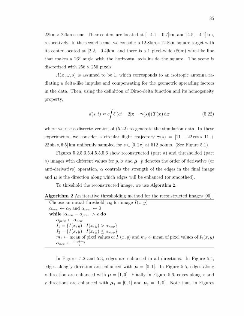
85
22km× 22km scene. Their centers are located at [−4.1,−0.7]km and [4.5,−4.1]km,
respectively. In the second scene, we consider a 12.8km×12.8km square target with
its center located at [2.2,−0.4]km, and there is a 1 pixel-wide (86m) wire-like line
that makes a 26 angle with the horizontal axis inside the square. The scene is
discretized with 256× 256 pixels.
A(x, ω, s) is assumed to be 1, which corresponds to an isotropic antenna ra-
diating a delta-like impulse and compensating for the geometric spreading factors
in the data. Then, using the definition of Dirac-delta function and its homogeneity
property,
d(s, t) ≈ c
∫δ (ct− 2|x− γ(s)|)T (x) dx (5.22)
where we use a discrete version of (5.22) to generate the simulation data. In these
experiments, we consider a circular flight trajectory γ(s) = [11 + 22 cos s, 11 +
22 sin s, 6.5] km uniformly sampled for s ∈ [0, 2π] at 512 points. (See Figure 5.1)
Figures 5.2,5.3,5.4,5.5,5.6 show reconstructed (part a) and thresholded (part
b) images with different values for p, α and µ. p denotes the order of derivative (or
anti-derivative) operation, α controls the strength of the edges in the final image
and µ is the direction along which edges will be enhanced (or smoothed).
To threshold the reconstructed image, we use Algorithm 2.
Algorithm 2 An iterative thresholding method for the reconstructed images [90].
Choose an initial threshold, α0 for image I(x, y)αnew ← α0 and αprev ← 0while |αnew − αprev| > ε do
αprev ← αnewI1 = I(x, y) : I(x, y) > αnewI2 = I(x, y) : I(x, y) ≤ αnewm1 ← mean of pixel values of I1(x, y) and m2 ←mean of pixel values of I2(x, y)αnew ← m1+m2
2
In Figures 5.2 and 5.3, edges are enhanced in all directions. In Figure 5.4,
edges along y-direction are enhanced with µ = [0, 1]. In Figure 5.5, edges along
x-direction are enhanced with µ = [1, 0]. Finally in Figure 5.6, edges along x and
y-directions are enhanced with µ1 = [0, 1] and µ2 = [1, 0]. Note that, in Figures

86
5.4, 5.5, 5.6 wire is not reconstructed since its direction is not along µ’s used in the
examples.
The numerical simulations show that the edges are enhanced (or smoothed)
in desired directions and the edges are reconstructed directly from the SAR data
successfully.
x (km)
y (k
m)
−10 −5 0 5 10
−10
−8
−6
−4
−2
0
2
4
6
8
10
0
0.1
0.2
0.3
0.4
0.5
0.6
0.7
0.8
0.9
1
(a)
x (km)
y (k
m)
−10 −5 0 5 10
−10
−8
−6
−4
−2
0
2
4
6
8
10
0
0.1
0.2
0.3
0.4
0.5
0.6
0.7
0.8
0.9
1
(b)
Figure 5.1: Imaging scenes used to generate the radar data.
5.5.2 Civilian Vehicles Dome Data Set
We use CV dome data set as a second set of simulations to demonstrate the
performance of the method [42]. In CV dome data set, SAR data is simulated for
various civilian vehicles by using high-fidelity electromagnetic wave simulating codes.
Cars are modeled by using realistic CAD models and electromagnetic properties of
different parts of the cars (glass, metallic, plastic etc.). The radar data provided
includes 5760 pulses with 512 frequency bins. The results are shown in Figures
5.7-5.10. We see that the edges are enhanced along desired directions.
5.6 Conclusion
In this chapter, we presented a novel edge detection method applicable directly
to SAR received signal. The method first filters the received data, and then back-
projects. The filter detects the edges of the scene in different directions at each pixel

87
Reconstructed Image : p = 1 α = 0.2
x (km)
y (k
m)
−10 −8 −6 −4 −2 0 2 4 6 8 10
−10
−8
−6
−4
−2
0
2
4
6
8
10
0
0.1
0.2
0.3
0.4
0.5
0.6
0.7
0.8
0.9
1
(a) Reconstructed image for the first scene.
Thresholding with intensity = 0.57
x (km)
y (k
m)
−10 −8 −6 −4 −2 0 2 4 6 8 10
−10
−8
−6
−4
−2
0
2
4
6
8
10
0
0.1
0.2
0.3
0.4
0.5
0.6
0.7
0.8
0.9
1
(b) Reconstructed image after thresholding forthe first scene.
Figure 5.2: Enhancement of edges in all directions for the first scene.
reconstructed. The method is computationally efficient and may be implemented
with the computational complexity of the fast-backprojection algorithms.

88
Reconstructed Image : p = 1 α = 0.8
x (km)
y (k
m)
−10 −8 −6 −4 −2 0 2 4 6 8 10
−10
−8
−6
−4
−2
0
2
4
6
8
10
0
0.1
0.2
0.3
0.4
0.5
0.6
0.7
0.8
0.9
1
(a) Reconstructed image for the secondscene.
Thresholding with intensity = 0.55
x (km)
y (k
m)
−10 −8 −6 −4 −2 0 2 4 6 8 10
−10
−8
−6
−4
−2
0
2
4
6
8
10
0
0.1
0.2
0.3
0.4
0.5
0.6
0.7
0.8
0.9
1
(b) Reconstructed image after thresholdingfor the second scene.
Figure 5.3: Enhancement of edges in all directions for the second scene.
Reconstructed Image : p = 2 α = 0.8
x (km)
y (k
m)
−10 −8 −6 −4 −2 0 2 4 6 8 10
−10
−8
−6
−4
−2
0
2
4
6
8
10
0
0.1
0.2
0.3
0.4
0.5
0.6
0.7
0.8
0.9
1
(a) Reconstructed image for the secondscene.
Thresholding with intensity = 0.68
x (km)
y (k
m)
−10 −8 −6 −4 −2 0 2 4 6 8 10
−10
−8
−6
−4
−2
0
2
4
6
8
10
0
0.1
0.2
0.3
0.4
0.5
0.6
0.7
0.8
0.9
1
(b) Reconstructed image after thresholdingfor the second scene.
Figure 5.4: Enhancement of edges in x-direction for scene 2 with µ = [1, 0].

89
Reconstructed Image : p = 1 α = 0.8
x (km)
y (k
m)
−10 −8 −6 −4 −2 0 2 4 6 8 10
−10
−8
−6
−4
−2
0
2
4
6
8
10
0
0.1
0.2
0.3
0.4
0.5
0.6
0.7
0.8
0.9
1
(a) Reconstructed image for the secondscene.
Thresholding with intensity = 0.7
x (km)
y (k
m)
−10 −8 −6 −4 −2 0 2 4 6 8 10
−10
−8
−6
−4
−2
0
2
4
6
8
10
0
0.1
0.2
0.3
0.4
0.5
0.6
0.7
0.8
0.9
1
(b) Reconstructed image after thresholdingfor the second scene.
Figure 5.5: Enhancement of edges in y-direction for scene 2 with µ = [0, 1].
Reconstructed Image : p = 1 α = 0.8
x (km)
y (k
m)
−10 −8 −6 −4 −2 0 2 4 6 8 10
−10
−8
−6
−4
−2
0
2
4
6
8
10
0
0.1
0.2
0.3
0.4
0.5
0.6
0.7
0.8
0.9
1
(a) Reconstructed image for the second scene.
Thresholding with intensity = 0.6
x (km)
y (k
m)
−10 −8 −6 −4 −2 0 2 4 6 8 10
−10
−8
−6
−4
−2
0
2
4
6
8
10
0
0.1
0.2
0.3
0.4
0.5
0.6
0.7
0.8
0.9
1
(b) Reconstructed image after thresholding forthe second scene.
Figure 5.6: Enhancement of edges in x and y-directions for scene 2 withµ1 = [1, 0] and µ2 = [0, 1].

90
(a) Reconstructed image for the Jeep data. (b) Reconstructed image after thresholding forthe Jeep data.
Figure 5.7: Original image reconstructed with FBP.
(a) Reconstructed image for the first scene. (b) Reconstructed image after thresholding forthe Jeep data.
Figure 5.8: Enhancement of edges in all directions.

91
(a) Reconstructed image for the first scene. (b) Reconstructed image after thresholding forthe Jeep data.
Figure 5.9: Enhancement of edges along x1 direction, i.e. µ = [1, 0].
(a) Reconstructed image for the Jeep data. (b) Reconstructed image after thresholding forthe Jeep data.
Figure 5.10: Enhancement of edges along x2 direction, i.e. µ = [0, 1].

CHAPTER 6
ITERATIVE ANALYTIC SAR INVERSION WITH
Lp-TYPE REGULARIZATION
In this chapter, we formulate the SAR image formation problem with non-quadratic
edge-preserving prior models and address the resulting optimization problems it-
eratively by sequences of FBP operators. These algorithms are computationally
efficient with the complexity equal to that of the fast-backprojection. Additionally,
they are applicable to the so-called interrupted SAR systems [93], [94] where data
samples are limited and measured data is corrupted by noise.
First, we develop an iterative reweighted-type SAR image formation algo-
rithm. SAR image reconstruction problem is modeled as an Lp-norm constrained
minimization problem. Then, we approximate this problem by a sequence of L2-
norm constrained quadratic minimization problems as inversions of the underlying
GRT. We approximate the solution of each optimization problem iteratively with
a sequence of analytic, FBP operators. At every iteration, we use the solution
obtained in the previous iteration to determine the filter of the next FBP operator.
Next, we develop an iterative shrinkage-type algorithm that is applicable to
limited data. The algorithm includes iterative applications of forward projection
and backprojection operators.
The methods that are developed in this chapter have the following advantages:
(1) They can be implemented efficiently using the fast-backprojection algorithms.
(2) They do not require a priori information. (3) They are applicable to a wide range
of image reconstruction problems including other SAR modalities, X-ray computed
tomography and acoustics where GRTs naturally arise. (4) They are particularly
suitable for SAR reconstruction with limited aperture.
We demonstrate the performance of the methods using both synthetic data
and the Civilian Vehicles (CV) dome data set provided by the Air Force Research
Laboratory (AFRL) [42] and compare its performance to those of the other state-
of-the-art sparse signal recovery techniques.
92

93
6.1 Introduction
SAR image reconstruction is a challenging problem. From a real world appli-
cation point of view, the challenge is threefold: (1) The amount of data collected for
a single acquisition may be very large to transmit and process in real time. As an
example, in Air Force Research Laboratories’ (AFRL) wide-angle SAR experiment,
2.718Gb/seconds data was collected over 647 seconds. This resulted in terabytes of
data [2]. Therefore, it is desirable to reduce the data needed for image reconstruc-
tion. (2) Measured data in many practical applications may be incomplete [35]–[38].
(3) Finally, there is a growing interest in SAR systems that are capable of operating
in multiple modes. These systems are referred to as the interrupted SAR systems
and have various operation modes such as imaging, target recognition and track-
ing [93]–[97]. Switching between different operation modes may result in missing or
incomplete data.
All these limitations require the development of high fidelity SAR image re-
construction with under-sampled or missing data. In addition to the undersampled
data, the noise is always present in the measurements. To address this, the sparse
signal recovery techniques offer a powerful approach and have been extensively used
in the SAR imaging community [98]–[102]. In [103], [104], it was shown that given
the knowledge about sparsity of a signal, i.e. the number of non-zero elements, the
signal may be reconstructed with fewer samples than the Nyquist theorem requires.
6.2 Related Work
Many solutions with performance guarantees are developed and presented in
recent years for sparse signal recovery. These methods can be broadly categorized
into four classes: (1) Lp-norm constrained optimization algorithms [30], [50]; (2)
greedy pursuits-type algorithms [88], [101], [105]–[112]; (3) iterative reweighted-
type algorithms (IRtA) [34], [113]–[115]; and (4) iterative shrinkage-type algorithms
(IStA) [116]–[128].
Within Lp-norm constrained optimization framework, Cetin et al. used Lp-
norm constraint for 0 < p ≤ 1 in [50] with a non-quadratic data fidelity term to
suppress noise and a total variation term to enhance features in the image. Kragh

94
et al. applied an iterative majorization-minimization scheme to a quadratic cost
function in [30].
A second class of algorithms for sparse signal recovery is the greedy-pursuits-
type algorithms. The basis pursuits (BP) [101], [111], [112], matching pursuits (MP)
[105] and orthogonal matching pursuits (OMP) [109] are widely used within this
class of algorithms. The BP algorithm decomposes a signal into a superposition of
dictionary elements by means of L1-norm minimization [101], [111], [112]. Mallat et
al. introduced the MP algorithm in [105]. Matching pursuits are used to decompose
signals into a linear expansion of waveforms that are selected from a redundant
dictionary of Gabor functions to give adaptive signal representations. Many greedy
algorithms are derived from the MP method. In [106], Burns et al. decomposed
radar signals using a dictionary of functions. In [33] an MP method was used with
a nonlinear iterative algorithm. In [32], another MP-based algorithm used a tree
search algorithm. In [109], Tropp used OMP to solve the sparse signal recovery
problem and unified the prior BP-based methods and extended them to OMP.
Another set of algorithms for the sparse signal recovery techniques is the iter-
ative reweighted-type algorithms. In [113], iterative reweighted least squares min-
imization procedures are used while forming the SAR image with a sequence of
L2-norm based minimizations to solve an L1-norm minimization problem. Bayesian
estimation techniques are also used within this framework [31], [53]. In [53], Vu et
al. proposed an approach similar to maximum a priori estimation with iterative
minimization procedures. In [115], Candes et al. solved a sequence of weighted
L1-norm minimization problems where the weights used for the next iteration are
calculated from the current solution with fewer measurements. In [114] algorithms
for optimal basis selection are derived by minimizing various diversity measures
such as Lp-norm, Gaussian and Shannon entropies. It was shown that the Gaussian
entropy minimization is equivalent to the L0-norm minimization problem. In [54],
the SAR image reconstruction problem was formulated as an Lp-norm constrained
quadratic inversion problem approximated with a sequence of L2-norm constrained
problems analytically.
The last set of algorithms belongs to the family of iterative shrinkage-type al-

95
gorithms, first introduced by Donoho et al. in [116]–[118]. Iterative shrinkage-type
algorithms can be considered as gradient-based algorithms for solving sparse signal
recovery problems via iterative multiplications with the underlying linear transfor-
mation matrices [126]. In radar imaging, this corresponds to iterative applications of
forward projection and backprojection operators. There are different derivations of
the iterative shrinkage-type of algorithms based on thresholding [126], expectation
maximization [121] and majorization-minimization [119], [120].
In this chapter, we develop novel iterative reweighted-type and shrinkage-type
algorithms to suppress noise that is applicable to limited data. For the rest of the
thesis, Lp-norm will correspond to the norms for 0 < p ≤ 1.
6.3 Sparse Signal Recovery Problem
The goal of the sparse signal recovery techniques is to solve an underdeter-
mined (or ill-conditioned) system of linear equations given by
FT + n = d (6.1)
where n is the measurement noise, F ∈ Rn×m, n < m is the linear transformation
matrix , T ∈ Rm is the “sparse” input signal to be recovered from the measurements
d ∈ Rn.
The objective of the sparse signal recovery techniques is to find T which solves
the equation given in (6.1) and has the minimum number of non-zero elements, i.e.
L0-norm. Therefore, the sparse recovery approach to solving (6.1) is given by
min |T|0 subject to |d− FT|22 ≤ ε (6.2)
where |n|22 < ε. This is an NP-hard problem [129].
As an alternative, under the conditions given in Appendix H, we can replace
L0-norm with Lp-norm and define
min |T|1 subject to |d− FT|22 ≤ ε (6.3)

96
for p = 1. (6.3) is a convex relaxation of (6.2) [109].
Another approach to address the problem stated in (6.3) consists of the follow-
ing [130]: (1) the minimization of an objective functional that includes a quadratic
error term to suppress noise, and (2) a sparsity inducing regularization term to
represent T. This approach results in the following optimization problem:
minT|d− FT|22 + λ1Tρ(T) (6.4)
where 1 ∈ Rn is a vector of ones; λ is the regularization parameter that determines
the trade-off between the sparsity and the residue d − FT; and ρ, Rm → R is
a sparsity inducing scalar-valued potential function that operates pointwise on its
argument.
6.4 Received Signal, Target, and Noise Models
As described in detail in the previous chapters, we can model the measurements
in many SAR systems as follows:
d(s, t) = F [T ](s, t) :=
∫eiΦ(ω,x,s,t)A(ω,x, s, t)T (x)dωdx (6.5)
where T (x) is the target to be recovered from the measurements d(s, t), A is the
amplitude function of the forward operator F , and
Φ(ω,x, s, t) = 2πω(t−R(s,x)/c) (6.6)
is the phase function. R(s,x) is a range function which takes different forms as
given in (2.17)-(2.19) depending on the SAR modality.
We assume that the measurements are corrupted by zero-mean Gaussian noise
n(s, t) and model the measured data as
d(s, t) = F [T ](s, t) + n(s, t). (6.7)

97
The autocovariance function of the noise is given by
E[n(s, t)n(s′, t′)] = σ2(s)δ(s− s′)Rn(t, t′) (6.8)
where
Rn(t, t′) =
∫ei2πω(t−t′)|Sn(ω)|2 dω. (6.9)
We refer to |Sn(ω)|2 as the power spectral density function of noise.
From a Bayesian estimation point of view, (6.4) can be considered as the max-
imum a posteriori (MAP) estimation of the unknown T with an appropriate prior
from the noisy measurements d [131]. Let pT(T |d = d), pd(d|T = T ), pT(T ), pd(d)
denote the a posteriori distribution of the target given the measurements, the dis-
tribution of the measurements given the target, the distribution of the target and
the distribution of the measurements, respectively. Using the Bayes’ Theorem, we
write
pT(T |d = d) =pd(d|T = T )pT(T )
pd(d)(6.10)
Let L(T |d) denote the log-likelihood of the a posteriori distribution of the target
scene given the measurements. Using (6.10), we can write
L(T |d = d) = L(d|T = T ) + log(pT(T ))− log(pd(d)). (6.11)
Using the MAP estimation, we can find an estimate for T as follows:
TMAP = maxT
L(T |d = d) (6.12)
= maxT
L(d = d|T ) + log(pT(T )) (6.13)
= maxT
L(d = d, T ), (6.14)
i.e. the MAP estimate maximizes the joint distribution as well [31]. When the prior
distribution is Gaussian then (6.4) corresponds to an MMSE estimate. However,
MMSE estimates result in over-blurred images if applied globally. We overcome this
shortcoming by applying MMSE criteria locally in Chapter 3. Here, we wish to

98
use sparsity promoting priors for pT to preserve edges of the reconstructed images.
The Markov random fields (MRF) offer a comprehensive framework to design such
priors [131], [132]. The probability distribution of an MRF can be expressed using
the Gibbs distribution as follows [131], [133]:
pT (T ) =1
Zexp
(−∑c∈C
ρc(Tc)
)(6.15)
where Z is a normalization constant, ρc is any function of a local group of points
c among all local groups of points C. Finally, under some conditions, Hammersley-
Clifford theorem states that a random field is an MRF if and only if its probability
distribution can be represented using the Gibbs distribution [134], [135].
There are many possible sparsity inducing potential functions for the choice
of ρ that are convex and non-convex. The ones that are investigated in this thesis
are listed in Table 6.1 [31], [136]–[143].
Table 6.1: Table showing the sparsity inducing potential functions, ρ(f)for an input function f investigated in the thesis.
Convex functions f2
1+f2 f 2 log(1 + f 2) |f |1+|f |
Non-convex functions |f | log cosh(f) min(|f |2, 2f − 1) |f |p |f |p1+fq−p
6.5 Analytic SAR Image Formation with Sparsity Promot-
ing Prior Models
6.5.1 Problem Definition
In Chapter 3, we describe a novel SAR inversion method based on locally
defined MMSE criterion. The method results in an FBP-type analytic reconstruction
technique in which the FBP filter requires second-order statistics of the target,
clutter and the noise. Furthermore, we estimate these parameters from the data as
described in Appendix E.

99
The MMSE criterion function inherently relies on the Gaussianity of the un-
derlying processes of the target, clutter and noise, hence the L2-norm. If applied
globally, the L2-norm minimization over-smooths the images resulting in loss of
features in reconstructed images. In this chapter, we develop an analytic inver-
sion method with the Lp-norm (p > 0) constraint. Furthermore, we approximate
the Lp-norm constrained inversion problem with a sequence of L2-norm constrained
inversion problems.
There are many sparse signal recovery techniques to solve the problem (6.4).
Using the target model described in the previous section and the prior exp(−ρ(T )),
we can address a solution to this problem by considering the following optimization
problem:
Jre(T ) = λ
∫ρ(T (z))dz +
1
2|d−F [T ]|22 (6.16)
where ρ is defined in the previous section and can be one of the functions listed in
Table 6.1. We will find solutions to solve (6.16) by using the techniques described
in [120], [123], [144]. It should be noted here that we can easily replace ρ(T (z))
with ρ(∇T (z)) to find a total-variations estimate for the target scene.
6.5.2 Approximate Solutions for the Optimization Function
6.5.2.1 Iterative Reweighted-type Analytic Reconstruction
For ρ(T ) = |T |pp,α, we write
T ∼ exp(−|T |pp,α) (6.17)
where
|T |pp,α =
∫|T (z)|p
α(z)dz < +∞, α(z) > 0. (6.18)
(6.17) can be considered as a MAP estimate of the target T , under a sparsity
inducing prior, i.e. Lp-norm. Similarly we can model a total variations estimate of

100
the target by using the following model:
∇T ∼ exp(−|∇T |pp,α). (6.19)
Using (6.17), the MAP estimation of T is equivalent to the optimization prob-
lem given by
P1 : minλ|T |pp,α + |d−F [T ]|22,Rn . (6.20)
In order to solve this optimization problem efficiently, we will convert P1 to a
sequence of quadratic problems P2 and solve each problem analytically. This will
result in an analytic and fast solution to Lp-norm constrained problem described
in (6.20). To do that, we will adapt the methodology described in [144] into our
problem formulation.
Let Tk, k = 0, 1, . . . be the solution of the P2 problem at the kth iteration.
Then, we define an operator Iqα,k−1 such that
Iqα,k−1T (z) =T (z)
α1/2(z)|Tk−1(z)|q. (6.21)
Instead of applying this operator on T , we apply it on an edge-enhanced version of
T to enhance features in the image:
P [T ](z) :=
∫Ωz
e−iξ·(z−x)(1 + |ξ|)T (x)dxdξ, (6.22)
P [T ](z) :=
∫Ωz
e−iξ·(z−x)Qe(z, ξ)d(s, t)dsdtdx (6.23)
where
|∇T (z)| ≈∫
Ωz
e−iξ·(z−x)|ξ|T (x)dxdξ (6.24)
as given in [145] and
Qe(z, ξ) = (1 + |ξ|)Q(z, ξ) (6.25)

101
acts as an unsharp masking filter.
By setting p = 2− 2q for (6.18)
Iqα,k−1T (z) =P [T ](z)
α1/2(z)|P [Tk−1](z)|1−p/2, (6.26)
|Iqα,k−1T (z)|22 =
∫ ∣∣∣∣P [T ](z)|P [Tk−1](z)|p/2
α1/2(z)P [Tk−1](z)
∣∣∣∣2 dz, (6.27)
|Iqα,k−1T (z)|22 =
∫ ∣∣∣∣ P [T ](z)
α1/2(z)|P [Tk−1](z)|
∣∣∣∣2 |P [Tk−1](z)|pdz. (6.28)
For |P [T (z)−P [Tk−1](z)| < ε where ε is a predetermined sufficiently small threshold,
we assume that |P[T ](z)|2|P[Tk−1](z)| ≈ 1. Therefore,
|Iqα,k−1T (z)|22 ≈∫|P [T ](z)|p
α(z)dz → |Iqα,k−1T (z)|22 ≈ |P [T ]|pp,α. (6.29)
and the modified optimization problem is given by
P2 : minλ|Iqα,k−1T (z)|22 + |g −F [T ]|22,Rn (6.30)
This way we convert the optimization problem given by P1 which includes an Lp-
norm to P2 which only includes an L2-norm. It should be noted here that T in
(6.30) can be effectively replaced with ρ(T ) and ρ(∇T ).
A pseudocode for SAR image reconstruction with limited data using IRtA is
given in Algorithm 3.
Algorithm 3 A pseudocode for IRtA.
1: Initialize f0 ≡ 1 on its support and k = 1 where ρ(P [T ](z)) is the edge-enhancedFBP image formed from the noisy data.
2: while |P [Tk]− P [Tk−1]|22 > ε do
3: Calculate Iqα,k−1T (z) = ρ(P[T ](z))|ρ(P[Tk−1](z))|q for q = 1/2.
4: Derive the edge-enhancing FBP filter Qk = minQk J(Qk) using (3.44) and[145].
5: Find P [Tk] = BQek[g].6: Update Iqα,k−1 → I
qα,k
7: k = k + 1
8: return Tk

102
6.5.2.2 Iterative Shrinkage-type Analytic Reconstruction
Iterative shrinkage-type algorithms (IStA) are another set of algorithms that
are used to solve the optimization problem given in (6.4) [116]–[128]. We can con-
sider IStA as gradient-based algorithms for solving (6.4) via iterative multiplications
with the matrix F and F† [126]. In radar imaging, this corresponds to repeated for-
ward and backprojections.
In the literature there are different derivations of IStA based on threshold-
ing [126], majorization-minimization [119], [120] and expectation maximization al-
gorithms [121]. In this section, we approach to solve the problem given in (6.4) by
using the proximal point and surrogate functions [120], and the fixed-point strat-
egy [123]. We define the following functional:
Js(T, T0) =c
2
(|T − T0|22 − |B†T − B†T0|22 − |B†(A− I)T |22
)(6.31)
to solve (6.4) where B is the backprojection operator (without any filtering), B† is
its adjoint, A is another operator whose kernel is the amplitude function A in (2.15)
and c > 0 is a constant chosen such that Js(T, T0) is strictly convex.
After adding Js to the objective function given in (6.16) and making some
simplifications, we form a new objective function:
Jsh(T ) = Jre(T ) + Js(T, T0) = 〈F †d− BB†T0 + cT0, f〉+ |T |22 + λ
∫ρ(T )dz + c1
(6.32)
where F is the forward operator given in (2.15) and F † is its adjoint.
Dividing (6.32) by c and adding |h0|2 where
h0 =1
c(F †d− BB†T0) + T0 (6.33)

103
we obtain
Jsh(T ) =1
2|T − h0|2 +
λ
c
∫ρ(T (z))dz + c2 (6.34)
=
∫ 1
2|T (z)− h0(z)|2 +
λ
cρ(T (z))
dz + c2. (6.35)
Similar to the derivation of the optimal filter (3.44), a Topt for which (6.34) is
minimized needs to be derived. To do that, the variation of Jsh is calculated with
respect to T by fixing some Tε and considering the variation, T + εTε for some small
ε:
d
dεJsh(T + εTε)
∣∣∣∣ε=0
= 0. (6.36)
Since the integrand in (6.34) is non-negative, Jsh is minimized whenever the inte-
grand is minimum. Therefore,
0 =d
dε
1
2|T + εTε − h0|2 +
λ
cρ(T + εfε)
∣∣∣∣ε=0
(6.37)
0 =d
dε
1
2|T − h0|2 +
1
2〈T − h0, εTε〉+
1
2|εTε|2 +
λ
cρ(T + εTε)
∣∣∣∣ε=0
(6.38)
0 =
1
2〈T − h0, Tε〉+ εTε +
λ
c〈ρ′(T + εTε), Tε〉
∣∣∣∣ε=0
(6.39)
0 =1
2(T − h0) +
λ
cρ′(T ) (6.40)
h0 =Topt +2λ
cρ′(Topt). (6.41)
where ρ′ stands for the gradient of the sparsity inducing potential function ρ. Possi-
ble choices for ρ are given in Table 6.1. A pseudocode for SAR image reconstruction
with IStA is given in Algorithm 4.

104
Algorithm 4 A pseudocode for IStA.
1: Initialize T0 ≡ 0, d = A†d on its support.2: while |P [Tk]− P [Tk−1]|22 > ε do3: Calculate the residual: rk = d− B†P [Tk]4: Backproject the residual and calculate hk: hk = Brk + P [Tk]5: Solve Tk+1 in hk = Tk+1 + 2λ
cρ′(P [Tk+1]).
6: Update the residual: rk+1 = d− B†P [Tk+1])7: k = k + 1
8: return Tk+1

105
6.6 Numerical Simulations
We consider two data sets to demonstrate the performance of the proposed
methods: A data set formed by using MATLAB and the Civilian Vehicle (CV)
Dome data set provided by AFRL [42]. For the first dataset, we perform two sets
of experiments:
1. Undersampled System: For a 22km×22km scene, we descritize the scene
into 128 × 128 pixels. We place a 5.16km×5.16km (30 pixels-by-30 pixels)
square at the scene center. A mono-static antenna traverses a circular tra-
jectory given by γ(s) = [11 cos s, 11 sin s, 6.5] km. The trajectory is uniformly
sampled for s ∈ [0, 2π] at 32 points. This is a much sparser sampling than
required. We sample the fast-time at 384 points. This corresponds to:
• 384× 32− by − 1 vector to represent the measurement data,
• 384× 32− by − 128× 128 matrix to represent the forward operator and
• 128× 128− by − 1 vector to represent the imaging scene.
Since 384× 32 is less than 128× 128, the inverse problem is underdetermined.
2. Regularly Sampled System: For a 22km×22km scene, we descritize the
scene into 64 × 64 pixels. We place a 7.9km×7.9km (23 pixels-by-23 pixels)
square at the scene center. A mono-static antenna traverses a circular tra-
jectory given by γ(s) = [11 cos s, 11 sin s, 6.5] km. The trajectory is uniformly
sampled for s ∈ [0, 2π] at 128 points. The fast-time is sampled with 543 points.
This corresponds to
• 543× 128− by − 1 vector to represent the measurement data,
• 543× 128− by − 64× 64 matrix to represent the forward operator and
• 64× 64− by − 1 vector to represent the imaging scene.
6.6.1 Numerical Simulations for IRtA with Synthetic Data
In these simulations, A(x, ω, s) is set to 1, which corresponds to the assumption
of an isotropic antenna radiating a Dirac-delta-like impulse and the compensation

106
of the geometric spreading in the measured data. We add Gaussian noise to the
projection data to simulate the thermal noise at an SNR level of 0dB. (See (3.54)
for a definition of SNR.) Then, we reconstruct the images with the limited data
using the Algorithm 3. We use the (3.44) with a known spectral density function for
the target. We use ten different potential functions given in Table 6.1 and evaluate
the performance of the algorithm for each potential function by considering the
following figures of merit:
1. Mean-square-error (MSE) between original target scene and the reconstructed
target image calculated by
MSE =1
MN
N∑i=1
M∑r=1
(T (xi)− Tr(xi)
)2
, (6.42)
where M is the number of realizations of the experiment, N is the number of
imaging grids Tr(x) is the reconstructed image in the rth realization.
2. The relative L2-norm difference, which we will refer to as the ∆-norm, between
the images that are reconstructed in consecutive iterations, calculated by
∆-norm =1
MNN∑i=1
M∑r=1
(Tr−1(xi)
)2
N∑i=1
M∑r=1
(Tr(xi)− Tr−1(xi)
)2
. (6.43)
3. Correlation of the range profiles of the reconstructed images with the range
profile of the true target scene (See Figure 6.3) calculated via Pearson’s cor-
relation coefficient [146]:
CORR =M∑r=1
cov(T rpr , Trp)
MσT rpr , σT rp(6.44)
where T rpr , T rp denote the range profiles of the reconstructed image at the rth
realization and the true target scene, respectively. “cov” denotes the covari-
ance and σ denotes the standard deviation.
Furthermore, ∆-norm is used to decide when the algorithm converges [50].

107
6.6.1.1 Numerical Simulations for the Under-Sampled Data
As a first set of experiments, we apply IRtA on the under-sampled data. Figure
6.1(a) shows the original target scene used for these simulations and Figure 6.1(b)
shows the FBP image when the SNR is 0dB. We perform these simulations ten times
for each potential function. It should be noted here that the algorithm converges
at different iterations for each potential function. Therefore, algorithm is run thirty
times for each objective function. Figure 6.2(a) shows the reconstructed image using
the deterministic FBP, which is the initialization to the algorithms. Figures 6.2(b)-
(f) show the reconstructed images using IRtA after the first, second, third, tenth
and the twentieth iterations, respectively. The numerical values for the convergence
of the algorithm for each potential function are reported in detail in Subsection 6.7.
20 40 60 80 100 120
20
40
60
80
100
120
0
0.1
0.2
0.3
0.4
0.5
0.6
0.7
0.8
0.9
1
(a)
20 40 60 80 100 120
20
40
60
80
100
120
0
0.1
0.2
0.3
0.4
0.5
0.6
0.7
0.8
0.9
1
(b)
Figure 6.1: (a) The original and (b) the reconstructed scene using thedeterministic FBP with a single realization. SNR is set to 0dB and theGaussian noise is added to the data to simulate the measurement noise.
When the SNR level is 0dB, i.e. when the noise power is comparable to the
signal power, the image reconstructed with FBP almost has no information about
the target. The target scene is vaguely visible and the background is noisy. However,
right after the first iteration (see Figure 6.2(b)), the target is visible even though
the initialization to the algorithm is the FBP image given in Figure 6.2(a) for all
possible potential functions. After several iterations, noise is suppressed around the
target and the features are more visible. Moreover, the noise is suppressed more in

108
20 40 60 80 100 120
20
40
60
80
100
120
0
0.1
0.2
0.3
0.4
0.5
0.6
0.7
0.8
0.9
1
(a)
20 40 60 80 100 120
20
40
60
80
100
120
0
0.1
0.2
0.3
0.4
0.5
0.6
0.7
0.8
0.9
1
(b)
20 40 60 80 100 120
20
40
60
80
100
120
0
0.1
0.2
0.3
0.4
0.5
0.6
0.7
0.8
0.9
1
(c)
20 40 60 80 100 120
20
40
60
80
100
120
0
0.1
0.2
0.3
0.4
0.5
0.6
0.7
0.8
0.9
1
(d)
20 40 60 80 100 120
20
40
60
80
100
120
0
0.1
0.2
0.3
0.4
0.5
0.6
0.7
0.8
0.9
1
(e)
20 40 60 80 100 120
20
40
60
80
100
120
0
0.1
0.2
0.3
0.4
0.5
0.6
0.7
0.8
0.9
1
(f)
Figure 6.2: The reconstructed images (a) using the deterministic FBP(initialization of the algorithm); and IRtA after (b) the first, (c) second,(d) third, (e) tenth, and (f) the twentieth iterations when the SNR is
0dB and ρ(f) = f2
1+f2 for the target in Figure 6.1.

109
0 20 40 60 80 100 120 1400
0.2
0.4
0.6
0.8
1(a)
0 20 40 60 80 100 120 1400
0.2
0.4
0.6
0.8
1(b)
Figure 6.3: The range profiles of the (a) reconstructed image at thetenth iteration, and (b) the true target scene in Figure 6.1(a).
the background.
Figure 6.4 shows the plots for the MSE, ∆-norm and correlation for the first
potential function ρ(f) = f2
f2+1. For the other objective functions, the patterns for
the plots are similar therefore they are not shown here. Figures 6.5 (a)-(c) show
the values of these metrics for all potential functions at every iteration as an image
grid. It is seen from the image given in Figure 6.5(b) that the ∆-norm, which is the
relative L2-norm difference between images that are reconstructed in consecutive
iterations, drops sharply after the first iteration and remains almost constant after
the second iteration. Similarly, we see in Figure 6.5(a) that the MSE between the
true and the reconstructed target images decreases sharply after the first iteration
and then remains constant. Finally, we show the correlation of the range profiles in
Figure 6.5 and observe that it increases right after the first iteration, then remains
almost constant for all of the potential functions.
Considering the results with different potential functions, potential function

110
0 5 10 15 20 25 300
0.02
0.04
0.06
MS
E
(a)
0 5 10 15 20 25 300
1
2
3
4
||f k−
f k−1|| 22 /||
f k−1|| 22
(b)
0 5 10 15 20 25 300.2
0.4
0.6
0.8
1
k−iteration number
Cor
rela
tion
(c)
Figure 6.4: The plots showing (a) the MSE between the original targetscene and the reconstructed target image for each iteration, (b) ∆-norm,
(c) correlation of the range profiles when ρ(f) = f2
1+f2 for IRtA and the
scene in Figure 6.1(a).
ρ(f) = min(f 2, 2f −1) results in the reconstructed images with the minimum MSE,
∆-norm and the maximum contrast while potential function fp
1+f2−p gives the results
with the maximum MSE, ∆-norm and the minimum contrast. Tables 6.2, 6.3, 6.4
show the values for MSE, ∆-norm, correlation respectively for the first five iterations
and each potential function. The rapid decrease in MSE, ∆-norm and the increase
in correlation is clearly seen in these tables.
6.6.1.2 Numerical Simulations for the Regularly Sampled Data
As a second set of experiments, we apply IRtA on regularly sampled data. We
perform these simulations ten times.
The algorithm converges at different iterations for each potential function.
Therefore, the algorithm is run thirty times for each potential function. Figure

111
Figure 6.5: Images showing (a) the MSE between original target sceneand the reconstructed target image for each iteration, (b) ∆-norm, (c)correlation of the range profiles for the target scene in Figure 6.1(a)
with all potential functions in the order of f2
1+f2 , f 2, log(1 + f 2), f1+f
, f ,
log cosh(T ), min(f 2, 2f − 1), f 1/2, f1/2
1+f2−1/2 for IRtA.

112
Table 6.2: The MSE between the true and the reconstructed target imagefor the first five iterations using IRtA for the target scene in Figure 6.1(a).The minimum values are shown in bold fonts.
Potential Iteration
Function 1 2 3 4 5f2
f2+15.331e-02 1.104e-02 9.486e-03 9.312e-03 9.122e-03
f 2 5.331e-02 9.996e-03 9.632e-03 8.892e-03 8.984e-03
log(f 2 + 1) 5.331e-02 1.048e-02 9.509e-03 9.091e-03 9.015e-03ff+1
5.331e-02 1.373e-02 1.136e-02 1.138e-02 1.127e-02
f 5.331e-02 1.281e-02 1.111e-02 1.096e-02 1.084e-02
log(cosh(f)) 5.331e-02 1.022e-02 9.420e-03 8.877e-03 8.967e-03
min(f 2, 2f − 1) 5.331e-02 4.495e-03 5.358e-03 4.184e-03 4.442e-03
fp 5.331e-02 1.366e-02 1.203e-02 1.178e-02 1.182e-02fp
1+f2−p 5.331e-02 1.332e-02 1.202e-02 1.214e-02 1.189e-02
∇f 5.331e-02 4.961e-03 6.886e-03 5.288e-03 5.715e-03
Table 6.3: The relative L2-norm difference between the images recon-structed at every iteration for the first five iterations using IRtA for thetarget scene in Figure 6.1(a). The minimum values are shown in boldfonts.
Potential Iteration
Function 1 2 3 4 5f2
f2+13.183 3.363e-02 7.702e-03 4.151e-03 2.550e-03
f 2 3.544 3.087e-02 1.044e-02 4.382e-03 2.281e-03
log(f 2 + 1) 3.360 2.812e-02 7.530e-03 3.659e-03 2.215e-03ff+1
2.461 3.777e-02 8.400e-03 5.392e-03 4.241e-03
f 2.659 3.159e-02 8.015e-03 4.189e-03 2.812e-03
log(cosh(f)) 3.451 2.743e-02 9.949e-03 5.036e-03 2.894e-03
min(f 2, 2f − 1) 1.454e+01 1.460e-01 4.344e-02 4.473e-03 9.142e-04
fp 2.454 2.919e-02 8.875e-03 5.232e-03 3.617e-03fp
1+f2−p 2.531 2.579e-02 8.626e-03 6.501e-03 4.966e-03
∇f 6.172 1.857e-02 1.243e-02 3.893e-03 3.680e-03

113
Table 6.4: The correlation of the true and the reconstructed target imagerange profiles for the first five iterations, using IRtA for the target scenein Figure 6.1(a). The maximum values are shown in bold fonts.
Potential Iteration
Function 1 2 3 4 5f2
f2+12.542e-01 6.295e-01 6.923e-01 6.824e-01 6.902e-01
f 2 2.542e-01 6.755e-01 6.975e-01 7.015e-01 7.007e-01
log(f 2 + 1) 2.542e-01 6.472e-01 6.955e-01 6.882e-01 6.947e-01ff+1
2.542e-01 5.542e-01 6.421e-01 6.251e-01 6.302e-01
f 2.542e-01 5.762e-01 6.505e-01 6.425e-01 6.471e-01
log(cosh(f)) 2.542e-01 6.644e-01 6.984e-01 6.944e-01 6.976e-01
min(f 2, 2f − 1) 2.542e-01 8.410e-01 8.045e-01 8.445e-01 8.316e-01
fp 2.542e-01 5.498e-01 6.350e-01 6.194e-01 6.202e-01fp
1+f2−p 2.542e-01 5.599e-01 6.307e-01 6.042e-01 6.086e-01
∇f 2.542e-01 8.237e-01 7.911e-01 8.331e-01 8.240e-01
10 20 30 40 50 60
10
20
30
40
50
60
0
0.1
0.2
0.3
0.4
0.5
0.6
0.7
0.8
0.9
1
(a)
10 20 30 40 50 60
10
20
30
40
50
60
0
0.1
0.2
0.3
0.4
0.5
0.6
0.7
0.8
0.9
1
(b)
Figure 6.6: (a) The original and (b) the reconstructed scene using thedeterministic FBP with a single realization. SNR is set to 0dB andGaussian noise is added to data to simulate the additive thermal noise.

114
10 20 30 40 50 60
10
20
30
40
50
60
0
0.1
0.2
0.3
0.4
0.5
0.6
0.7
0.8
0.9
1
(a)
10 20 30 40 50 60
10
20
30
40
50
60
0
0.1
0.2
0.3
0.4
0.5
0.6
0.7
0.8
0.9
1
(b)
10 20 30 40 50 60
10
20
30
40
50
60
0
0.1
0.2
0.3
0.4
0.5
0.6
0.7
0.8
0.9
1
(c)
10 20 30 40 50 60
10
20
30
40
50
60
0
0.1
0.2
0.3
0.4
0.5
0.6
0.7
0.8
0.9
1
(d)
10 20 30 40 50 60
10
20
30
40
50
60
0
0.1
0.2
0.3
0.4
0.5
0.6
0.7
0.8
0.9
1
(e)
10 20 30 40 50 60
10
20
30
40
50
60
0
0.1
0.2
0.3
0.4
0.5
0.6
0.7
0.8
0.9
1
(f)
Figure 6.7: The reconstructed images (a) using the deterministic FBP(initialization of the algorithm); and IRtA (b) after the first, (c) second,(d) third, (e) tenth, and (f) twentieth iterations when the SNR is 0dB
and ρ(f) = f2
1+f2 for the target in Figure 6.6.

115
0 10 20 30 40 50 60 70−0.2
0
0.2
0.4
0.6
0.8
0 10 20 30 40 50 60 700
0.2
0.4
0.6
0.8
1
Figure 6.8: The range profiles of the (a) reconstructed image at the tenthiteration, and (b) the true target scene in Figure 6.6(a).
6.7(a) shows the reconstructed image using the deterministic FBP, which is the ini-
tialization to the algorithms. Figures 6.7(b)-(f) show the reconstructed images using
IRtA after the first, second, third, tenth and the twentieth iterations, respectively
when the target scene is Figure 6.6(a) for the potential function ρ(f) = f2
f2+1.
When the SNR level is 0dB, again the image reconstructed with FBP almost
has no information about the target. The target scene is not visible and noisy.
After the first iteration (see Figure 6.7(b)), the target is visible even though the
initialization to the algorithm is the FBP image given in Figure 6.7(a). After several
iterations, noise is suppressed around the target and the features are more visible.
Moreover, the noise is suppressed more in the background.
In assessing the quality of the reconstructed images, we consider three figures
of merit: MSE, ∆-norm and the correlation of the range profiles with a rectangular
window defined earlier.
Figure 6.9 shows the plots for the MSE, ∆-norm and correlation for the first

116
0 5 10 15 20 25 300
0.02
0.04
0.06
MS
E
(a)
0 5 10 15 20 25 300
1
2
3
4
||f k−
f k−1|| 22 /||
f k−1|| 22
(b)
0 5 10 15 20 25 300.2
0.4
0.6
0.8
1
k−iteration number
Cor
rela
tion
(c)
Figure 6.9: The plots showing (a) the MSE between original target sceneand the reconstructed target image for each iteration, (b) ∆-norm, (c)
correlation of the range profiles when ρ(f) = f2
1+f2 for IRtA and the scene
in Figure 6.6(a).
potential function ρ(f) = f2
f2+1. For the other objective functions, the patterns for
the plots are similar therefore they are not shown here. Figures 6.10 (a)-(c) show the
values of these metrics for all potential functions at every iteration as an image grid.
We observe from Figure 6.10(b) that the value of the ∆-norm, drops sharply after
the first iteration and remains almost constant after the second iteration. Similarly,
we see in Figure 6.10(a) that the MSE between the original target scene and the
reconstructed image decreases sharply after the first iteration and remains almost
constant for higher iteration numbers. Finally, we show the correlation of the range
profiles in Figure 6.10. We observe that the correlation increases right after the first
iteration, then remains almost constant for higher number of iterations for all of the
potential functions.
Comparing the results for different potential functions, unlike the simulations

117
Figure 6.10: Images showing (a) the MSE between original target sceneand the reconstructed target image for each iteration, (b) ∆-norm, (c)correlation of the range profiles for the target scene in Figure 6.6(a)
with all potential functions in the order of f2
1+f2 , f 2, log(1 + f 2), f1+f
, f ,
log cosh(T ), min(f 2, 2f − 1), f 1/2, f1/2
1+f2−1/2 for IRtA.

118
performed in the previous subsection, we conclude that any one of the potential
functions does not result in better reconstructed images than the rest for all metrics.
Tables 6.5, 6.6, 6.7 show the values for MSE, ∆-norm, correlation, respectively for
the first five iterations and each potential function. min(f 2, 2f − 1) and fp
1+f2−p
perform slightly better considering the correlation values. The rapid decrease in the
MSE, ∆-norm and the increase in the correlation are clearly seen in these results.
Table 6.5: The MSE between the true and the reconstructed target imagefor the first five iterations using IRtA for the target scene in Figure 6.6(a).The minimum values are shown in bold fonts.
Potential Iteration
Function 1 2 3 4 5f2
f2+15.632e-02 3.021e-03 4.474e-03 2.909e-03 3.359e-03
f 2 5.632e-02 2.906e-03 4.656e-03 2.787e-03 3.429e-03
log(f 2 + 1) 5.632e-02 2.969e-03 4.572e-03 2.832e-03 3.366e-03ff+1
5.632e-02 3.460e-03 3.854e-03 3.244e-03 3.521e-03
f 5.632e-02 3.206e-03 4.196e-03 3.415e-03 3.536e-03
log(cosh(f)) 5.632e-02 2.955e-03 4.509e-03 2.739e-03 3.338e-03
min(f 2, 2f − 1) 5.632e-02 2.580e-03 3.988e-03 2.829e-03 3.117e-03
fp 5.632e-02 3.595e-03 4.138e-03 3.361e-03 3.557e-03fp
1+f2−p 5.632e-02 4.241e-03 3.797e-03 3.389e-03 3.402e-03
∇f 5.632e-02 9.468e-03 1.005e-02 9.062e-03 9.434e-03

119
Table 6.6: The relative L2-norm difference between the images recon-structed at every iteration for the first five iterations using IRtA for thetarget scene in Figure 6.6(a). The minimum values are shown in boldfonts.
Potential Iteration
Function 1 2 3 4 5f2
f2+12.913 4.035e-02 2.000e-02 1.180e-02 2.492e-03
f 2 2.917 4.396e-02 1.295e-02 4.340e-03 1.286e-03
log(f 2 + 1) 2.908 4.122e-02 1.353e-02 6.509e-03 1.551e-03ff+1
2.855 2.108e-02 4.640e-03 1.497e-03 5.400e-04
f 2.873 2.705e-02 1.300e-02 4.265e-03 1.476e-03
log(cosh(f)) 2.921 4.592e-02 1.323e-02 5.652e-03 1.414e-03
min(f 2, 2f − 1) 4.239 3.744e-02 9.151e-03 1.181e-03 3.339e-04
fp 2.819 2.648e-02 5.627e-03 9.382e-04 3.165e-04fp
1+f2−p 2.850 3.310e-02 8.373e-03 3.649e-03 3.136e-03
∇f 1.805 3.952e-02 1.536e-02 5.372e-03 3.037e-03
Table 6.7: The correlation of the true and the reconstructed target imagerange profiles for the first five iterations, using IRtA for the target scenein Figure 6.6(a). The maximum values are shown in bold fonts.
Potential Iteration
Function 1 2 3 4 5f2
f2+13.964e-01 8.021e-01 7.691e-01 7.976e-01 7.872e-01
f 2 3.964e-01 8.026e-01 7.600e-01 8.002e-01 7.793e-01
log(f 2 + 1) 3.964e-01 8.017e-01 7.640e-01 7.988e-01 7.850e-01ff+1
3.964e-01 8.014e-01 7.930e-01 7.982e-01 8.042e-01
f 3.964e-01 8.021e-01 7.803e-01 8.035e-01 7.904e-01
log(cosh(f)) 3.964e-01 8.024e-01 7.605e-01 8.012e-01 7.826e-01
min(f 2, 2f − 1) 3.964e-01 8.098e-01 7.907e-01 8.032e-01 7.989e-01
fp 3.964e-01 8.005e-01 7.846e-01 7.928e-01 7.921e-01fp
1+f2−p 3.964e-01 8.045e-01 7.935e-01 8.058e-01 8.064e-01
∇f 3.964e-01 7.325e-01 7.210e-01 7.372e-01 7.286e-01

120
6.6.2 Numerical Simulations for IStA with Synthetic Data
6.6.2.1 Numerical Simulations for the Under-Sampled Data
For this set of simulations, we use the target in 6.1(a). We apply the Algorithm
4 to suppress the noise and to reconstruct images using limited data. We use 10
different potential functions given in Subsection 6.5.1 with IStA.
As noted in the previous subsection, the algorithm converges at different it-
erations for each objective function and the algorithms is run thirty times for each
potential function. Figure 6.11(a) shows the reconstructed image using the deter-
ministic FBP, which is the initialization to the algorithms. Figures 6.11(b)-(f) show
the reconstructed images using IStA after the first, second, third, tenth and the
twentieth iterations, respectively for the potential function ρ(f) = f2
f2+1. When the
SNR level is 0dB the target is not visible in the image reconstructed with determin-
istic FBP. After the first iteration algorithm performs the following operation:
f1 ≈ T0 + B(d− B†T0)− 2λ
cρ′(T0) (6.45)
where f0 corresponds to the FBP image. The image is blurred since the algorithm
reconstructs images via backprojection without filtering. However, right after the
second iteration the shape of the target is revealed, but somewhat smooth. As more
iterations, are performed the level of smoothness decreases and the structure of the
target becomes more visible.
Figure 6.12 shows the MSE, ∆-norm and correlation plots for the potential
function ρ(f) = f2
f2+1. For the other objective functions, the patterns for the plots
are similar, therefore they are not shown here. Figures 6.13 (a)-(c) show the val-
ues of these metrics for all potential functions at every iteration on an image grid.
The plots in Figure 6.12(a) show that the relative L2-norm difference between the
images reconstructed in consecutive iterations drops sharply after the second itera-
tion. However, the MSE and ∆-norm fluctuate. Note that the algorithm attempts
to reduce the residual. However, when the residual is large, the algorithm attempts
to smooth the image aggressively in the next iteration. After that, the algorithm
attempts to compensate for the over-smoothing by using the original noisy radar

121
20 40 60 80 100 120
20
40
60
80
100
120
0
0.1
0.2
0.3
0.4
0.5
0.6
0.7
0.8
0.9
1
(a)
20 40 60 80 100 120
20
40
60
80
100
120
0
0.1
0.2
0.3
0.4
0.5
0.6
0.7
0.8
0.9
1
(b)
20 40 60 80 100 120
20
40
60
80
100
120
0
0.1
0.2
0.3
0.4
0.5
0.6
0.7
0.8
0.9
1
(c)
20 40 60 80 100 120
20
40
60
80
100
120
0
0.1
0.2
0.3
0.4
0.5
0.6
0.7
0.8
0.9
1
(d)
20 40 60 80 100 120
20
40
60
80
100
120
0
0.1
0.2
0.3
0.4
0.5
0.6
0.7
0.8
0.9
1
(e)
20 40 60 80 100 120
20
40
60
80
100
120
0
0.1
0.2
0.3
0.4
0.5
0.6
0.7
0.8
0.9
1
(f)
Figure 6.11: The reconstructed images (a) using the deterministic FBP(initialization of the algorithm); and IStA (b) after the first, (c) second,(d) third, (e) tenth, and (f) twentieth iterations when the SNR is 0dB
and ρ(f) = f2
1+f2 for the target in Figure 6.1.

122
0 5 10 15 20 25 300
0.02
0.04
0.06
0.08
MS
E
(a)
0 5 10 15 20 25 300
10
20
30
||f k−
f k−1|| 22 /||
f k−1|| 22
(b)
0 5 10 15 20 25 300
0.5
1
k−iteration number
Cor
rela
tion
(c)
Figure 6.12: The plots showing (a) the MSE between original target sceneand the reconstructed target image for each iteration, (b) ∆-norm, (c)
correlation of the range profiles when ρ(f) = f2
1+f2 for IStA and the scene
in Figure 6.1(a).
data. This increases the MSE as compared to that of the previous iteration. Hence,
MSE and ∆-norm values fluctuate from one iteration to the next.
The algorithm is run for thirty iterations in order to compare its performance
with that of the iterative reweighted-type reconstruction algorithm. The algorithm
converges around the fifth iteration almost for all the objective functions. Addi-
tional iterations result in degradation in the image quality as well as the loss in the
correlation.
Unlike IRtA, the type of the potential function used in the algorithm does not
affect performance as can be seen in Figures 6.13. Nevertheless, potential function
given by ρ(f) = min(f 2, 2f − 1), results in reconstructed images with the minimum
MSE and the maximum contrast. Tables 6.8, 6.9, 6.10 show the values of the MSE,
∆-norm and the correlation, respectively for the first five iterations and for each

123
Figure 6.13: Images showing (a) the MSE between original target sceneand the reconstructed target image for each iteration, (b) ∆-norm, (c)correlation of the range profiles for the target scene in Figure 6.1(a)
with all potential functions in the order of f2
1+f2 , f 2, log(1 + f 2), f1+f
, f ,
log cosh(T ), min(f 2, 2f − 1), f 1/2, f1/2
1+f2−1/2 for IStA.

124
potential function.
Table 6.8: The MSE between the true and the reconstructed target imagefor the first five iterations using IStA for the target scene in Figure 6.1(a).The minimum values are shown in bold fonts.
Potential Iteration
Function 1 2 3 4 5f2
f2+16.992e-02 9.129e-03 2.427e-02 1.638e-02 3.140e-03
f 2 6.992e-02 9.131e-03 2.431e-02 1.637e-02 3.134e-03
log(f 2 + 1) 6.992e-02 9.130e-03 2.429e-02 1.637e-02 3.137e-03ff+1
6.992e-02 9.123e-03 2.431e-02 1.632e-02 3.112e-03
f 6.992e-02 9.123e-03 2.442e-02 1.626e-02 3.086e-03
log(cosh(f)) 6.992e-02 9.130e-03 2.422e-02 1.641e-02 3.155e-03
min(f 2, 2f − 1) 6.992e-02 9.115e-03 2.469e-02 1.608e-02 3.011e-03
fp 6.992e-02 9.123e-03 2.442e-02 1.626e-02 3.086e-03fp
1+f2−p 6.992e-02 9.123e-03 2.431e-02 1.632e-02 3.112e-03
∇f 6.992e-02 9.126e-03 2.428e-02 1.635e-02 3.131e-03
6.6.2.2 Numerical Simulations for the Regularly Sampled Data
As a second set of experiments, we apply the IStA on regularly sampled data.
Algorithm is run thirty times for each potential function. Figure 6.14(a) shows
the reconstructed image using the deterministic FBP, which is the initialization
to the algorithms. Figures 6.14(b)-(f) show the reconstructed images using IStA
after the first, second, third, tenth and the twentieth iterations, respectively for the
potential function ρ(f) = f2
f2+1. After the first iteration, the image is blurred since
the algorithm reconstructs images via backprojection without filtering. However,
right after the second iteration the shape of the target is revealed but somewhat
smooth. More iterations reduce the over-smoothing and the high frequency content
of the target becomes more visible.
Figure 6.15 shows the plots for the MSE, ∆-norm and the correlation for the
potential function ρ(f) = f2
f2+1. For the other potential functions, the patterns for
the plots are similar, therefore they are not shown here. Figures 6.16 (a)-(c) show the

125
Table 6.9: The relative L2-norm difference between the images recon-structed at every iteration for the first five iterations using IStA for thetarget scene in Figure 6.1(a). The minimum values are shown in boldfonts.
Potential Iteration
Function 1 2 3 4 5f2
f2+12.944e+01 9.113 4.098 5.516e-01 6.000e-01
f 2 2.942e+01 9.145 4.088 5.526e-01 5.999e-01
log(f 2 + 1) 2.943e+01 9.127 4.094 5.520e-01 6.000e-01ff+1
2.938e+01 9.155 4.075 5.555e-01 6.031e-01
f 2.930e+01 9.247 4.041 5.598e-01 6.046e-01
log(cosh(f)) 2.947e+01 9.071 4.115 5.494e-01 5.988e-01
min(f 2, 2f − 1) 2.908e+01 9.490 3.947 5.732e-01 6.085e-01
fp 2.930e+01 9.247 4.041 5.598e-01 6.046e-01fp
1+f2−p 2.938e+01 9.155 4.075 5.555e-01 6.031e-01
∇f 2.942e+01 9.119 4.090 5.526e-01 6.005e-01
Table 6.10: The correlation of the true and the reconstructed target imagerange profiles for the first five iterations, using IStA for the target scenein Figure 6.1(a). The maximum values are shown in bold fonts.
Potential Iteration
Function 1 2 3 4 5f2
f2+11.760e-01 7.679e-01 9.099e-01 9.163e-01 9.258e-01
f 2 1.760e-01 7.679e-01 9.099e-01 9.164e-01 9.259e-01
log(f 2 + 1) 1.760e-01 7.679e-01 9.099e-01 9.163e-01 9.259e-01ff+1
1.760e-01 7.680e-01 9.099e-01 9.163e-01 9.258e-01
f 1.760e-01 7.679e-01 9.098e-01 9.163e-01 9.258e-01
log(cosh(f)) 1.760e-01 7.680e-01 9.099e-01 9.163e-01 9.258e-01
min(f 2, 2f − 1) 1.760e-01 7.678e-01 9.096e-01 9.163e-01 9.258e-01
fp 1.760e-01 7.679e-01 9.098e-01 9.163e-01 9.258e-01fp
1+f2−p 1.760e-01 7.680e-01 9.099e-01 9.163e-01 9.258e-01
∇f 1.760e-01 7.679e-01 9.101e-01 9.163e-01 9.258e-01

126
10 20 30 40 50 60
10
20
30
40
50
60
0
0.1
0.2
0.3
0.4
0.5
0.6
0.7
0.8
0.9
1
(a)
10 20 30 40 50 60
10
20
30
40
50
60
0
0.1
0.2
0.3
0.4
0.5
0.6
0.7
0.8
0.9
1
(b)
10 20 30 40 50 60
10
20
30
40
50
60
0
0.1
0.2
0.3
0.4
0.5
0.6
0.7
0.8
0.9
1
(c)
10 20 30 40 50 60
10
20
30
40
50
60
0
0.1
0.2
0.3
0.4
0.5
0.6
0.7
0.8
0.9
1
(d)
10 20 30 40 50 60
10
20
30
40
50
60
0
0.1
0.2
0.3
0.4
0.5
0.6
0.7
0.8
0.9
1
(e)
10 20 30 40 50 60
10
20
30
40
50
60
0
0.1
0.2
0.3
0.4
0.5
0.6
0.7
0.8
0.9
1
(f)
Figure 6.14: The reconstructed images (a) using the deterministic FBP(initialization of the algorithm); and IStA (b) after the first, (c) second,(d) third, (e) tenth, and (f) twentieth iterations when the SNR is 0dB
and ρ(f) = f2
1+f2 for the target in Figure 6.6.
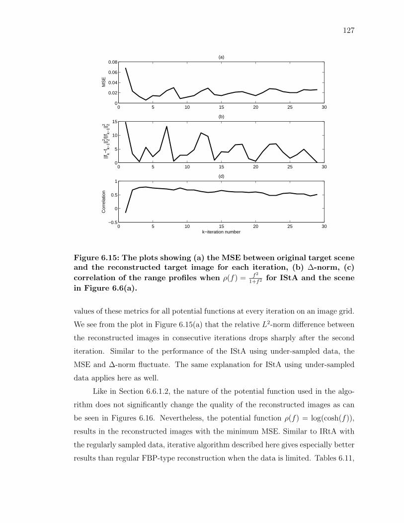
127
0 5 10 15 20 25 300
0.02
0.04
0.06
0.08
MS
E
(a)
0 5 10 15 20 25 300
5
10
15
||f k−
f k−1|| 22 /||
f k−1|| 22
(b)
0 5 10 15 20 25 30−0.5
0
0.5
1
k−iteration number
Cor
rela
tion
(d)
Figure 6.15: The plots showing (a) the MSE between original target sceneand the reconstructed target image for each iteration, (b) ∆-norm, (c)
correlation of the range profiles when ρ(f) = f2
1+f2 for IStA and the scene
in Figure 6.6(a).
values of these metrics for all potential functions at every iteration on an image grid.
We see from the plot in Figure 6.15(a) that the relative L2-norm difference between
the reconstructed images in consecutive iterations drops sharply after the second
iteration. Similar to the performance of the IStA using under-sampled data, the
MSE and ∆-norm fluctuate. The same explanation for IStA using under-sampled
data applies here as well.
Like in Section 6.6.1.2, the nature of the potential function used in the algo-
rithm does not significantly change the quality of the reconstructed images as can
be seen in Figures 6.16. Nevertheless, the potential function ρ(f) = log(cosh(f)),
results in the reconstructed images with the minimum MSE. Similar to IRtA with
the regularly sampled data, iterative algorithm described here gives especially better
results than regular FBP-type reconstruction when the data is limited. Tables 6.11,

128
Figure 6.16: Images showing (a) the MSE between original target sceneand the reconstructed target image for each iteration, (b) ∆-norm, (c)correlation of the range profiles for the target scene in Figure 6.6(a)
with all potential functions in the order of f2
1+f2 , f 2, log(1 + f 2), f1+f
, f ,
log cosh(T ), min(f 2, 2f − 1), f 1/2, f1/2
1+f2−1/2 for IStA.

129
6.12, 6.13 show the values for the MSE, ∆-norm and the correlation, respectively
for the first five iterations and each potential function.
Table 6.11: The MSE between the true and the reconstructed targetimage for the first five iterations using IStA for the target scene in Figure6.6(a). The minimum values are shown in bold fonts.
Potential Iteration
Function 1 2 3 4 5f2
f2+16.889e-02 2.350e-02 1.226e-02 5.636e-03 1.433e-02
f 2 6.890e-02 2.351e-02 1.225e-02 5.709e-03 1.442e-02
log(f 2 + 1) 6.889e-02 2.350e-02 1.226e-02 5.667e-03 1.437e-02ff+1
6.890e-02 2.350e-02 1.216e-02 5.733e-03 1.427e-02
f 6.891e-02 2.351e-02 1.209e-02 5.922e-03 1.439e-02
log(cosh(f)) 6.889e-02 2.350e-02 1.231e-02 5.562e-03 1.429e-02
min(f 2, 2f − 1) 6.894e-02 2.354e-02 1.184e-02 6.492e-03 1.457e-02
fp 6.891e-02 2.351e-02 1.209e-02 5.922e-03 1.439e-02fp
1+f2−p 6.890e-02 2.350e-02 1.216e-02 5.733e-03 1.427e-02
∇f 6.890e-02 2.349e-02 1.222e-02 5.660e-03 1.425e-02

130
Table 6.12: The relative L2-norm difference between the images recon-structed at every iteration for the first five iterations using IStA for thetarget scene in Figure 6.6(a). The minimum values are shown in boldfonts.
Potential Iteration
Function 1 2 3 4 5f2
f2+11.491e+01 3.304 4.656e-01 5.535 2.176
f 2 1.490e+01 3.305 4.704e-01 5.584 2.248
log(f 2 + 1) 1.491e+01 3.304 4.677e-01 5.556 2.207ff+1
1.490e+01 3.276 4.709e-01 5.525 2.136
f 1.488e+01 3.257 4.826e-01 5.598 2.213
log(cosh(f)) 1.492e+01 3.317 4.608e-01 5.510 2.154
min(f 2, 2f − 1) 1.482e+01 3.184 5.139e-01 5.706 2.277
fp 1.488e+01 3.257 4.826e-01 5.598 2.213fp
1+f2−p 1.490e+01 3.276 4.709e-01 5.525 2.136
∇f 1.490e+01 3.290 4.664e-01 5.500 2.131
Table 6.13: The correlation of the true and the reconstructed target imagerange profiles for the first five iterations, using IStA for the target scenein Figure 6.6(a). The maximum values are shown in bold fonts.
Potential Iteration
Function 1 2 3 4 5f2
f2+1-1.539e-01 6.847e-01 7.687e-01 7.927e-01 7.538e-01
f 2 -1.539e-01 6.846e-01 7.700e-01 7.950e-01 7.565e-01
log(f 2 + 1) -1.539e-01 6.847e-01 7.692e-01 7.937e-01 7.550e-01ff+1
-1.539e-01 6.848e-01 7.674e-01 7.906e-01 7.519e-01
f -1.538e-01 6.847e-01 7.686e-01 7.928e-01 7.552e-01
log(cosh(f)) -1.539e-01 6.847e-01 7.686e-01 7.924e-01 7.531e-01
min(f 2, 2f − 1) -1.537e-01 6.845e-01 7.696e-01 7.948e-01 7.588e-01
fp -1.538e-01 6.847e-01 7.686e-01 7.928e-01 7.552e-01fp
1+f2−p -1.539e-01 6.848e-01 7.674e-01 7.906e-01 7.519e-01
∇f -1.539e-01 6.847e-01 7.676e-01 7.911e-01 7.522e-01

131
6.6.3 Numerical Simulations for Lp-norm Regularization with CV Dome
Data Set
We perform a second set of simulations to demonstrate the performance of the
methods using the CV dome data set [42]. This data set was generated by AFRL.
The SAR data were simulated for various civilian vehicles by using high-fidelity
electromagnetic wave simulation codes. The cars were modeled by using realistic
CAD models and the electromagnetic properties of the different parts of the cars
(glass, metallic, plastic etc.). The radar data provided includes 5760 pulses with
512 frequency bins. Note that this dataset does not include measurement noise.
Therefore, Gaussian noise is added to the data at a 20dB SNR. To show that the
algorithms work well with limited data, we use only the 10% of the data. Therefore,
the size of the data is 576 × 512. The results are provided in Figures 6.18(a)-(d)
using IRtA, 6.20(a)-(d) and 6.21(a)-(b) using IStA.
50 100 150 200
50
100
150
200
250
300 0
0.1
0.2
0.3
0.4
0.5
0.6
0.7
0.8
0.9
1
(a)
2 4 6 8 10
2
4
6
8
10
12
14
16
18
20
0.05
0.1
0.15
0.2
0.25
0.3
0.35
(b)
Figure 6.17: (a) The reconstructed Jeep image via FBP using the entireCV dome data set and (b) the left-bottom corner of the car that is usedin correlation calculations.
Figure 6.17(a) shows the original target scene reconstructed using the deter-
ministic FBP and the full aperture data without any noise. Figure 6.18(a) shows

132
50 100 150 200
50
100
150
200
250
300 0
0.1
0.2
0.3
0.4
0.5
0.6
0.7
0.8
0.9
1
(a)
50 100 150 200
50
100
150
200
250
300 0
0.1
0.2
0.3
0.4
0.5
0.6
0.7
0.8
0.9
1
(b)
50 100 150 200
50
100
150
200
250
300 0
0.1
0.2
0.3
0.4
0.5
0.6
0.7
0.8
0.9
1
(c)
50 100 150 200
50
100
150
200
250
300 0
0.1
0.2
0.3
0.4
0.5
0.6
0.7
0.8
0.9
1
(d)
Figure 6.18: The reconstructed SAR images for the CV dome data setusing (a) the deterministic FBP; and IRtA after (b) the first, (c) second,and (d) the tenth iterations, respectively when the SNR is 20dB andρ(f) = ∇f .

133
1 2 3 4 5 6 7 8 94.55
4.6
4.65
4.7x 10
−3
MS
E
(a)
1 2 3 4 5 6 7 8 90
0.01
0.02
0.03
0.04
||f k−
f k−1|| 22 /||
f k−1|| 22
(b)
1 2 3 4 5 6 7 8 9 10
0.4
0.5
0.6
0.7
k−iteration number
Cor
rela
tion
(c)
Figure 6.19: (a) The MSE between the original target scene and thereconstructed target image for each iteration, (b) the ∆-norm, (c) thecorrelation of the reconstructed image patch shown in Figure 6.17(b)using IRtA and the CV dome data set when the SNR is 20dB and ρ(f) =∇f .
the reconstructed image using the deterministic FBP. Figures 6.18(b)-(d) shows the
reconstructed images after the first, second and the fifth iterations, respectively
at 20dB SNR using IRtA. The image reconstructed using the deterministic FBP
is noisy and contains limited aperture artifacts. These artifacts are the strongest
around the corners of the vehicle. However, right after the first iteration, the target
becomes visible. We can clearly see the artifact suppression around the corners of
the car.
The plots in Figures 6.19(a)-(c) show the MSE between the true and the re-
constructed target image, the relative L2-norm difference between the images recon-
structed in consecutive iterations, the correlation of the reconstructed image with
the patch shown in Figure 6.17(b) when ρ(f) = ∇f using IRtA and the CV dome
data set. It is seen that the ∆-norm drops sharply after the first iteration and

134
remains almost constant after the fourth iteration. Similarly, as in Figure 6.19(a),
the MSE between the original target scene and the reconstructed image sharply
decreases after the first iteration, but then fluctuates at every iteration. As can
be seen in Table 6.14, the algorithm converges after the third iteration (see Figure
6.23(a)) and additional iterations may result in increase in the MSE.
Table 6.14: The MSE, ∆-norm and the correlation values using IRtA andthe CV dome data set for 10 iterations. The tolerance for the IRtA isset to ∆-norm less than 1e− 3. The row in bold fonts shows the iterationstep at which the algorithm converges.
Iteration MSE ∆-norm Correlation
1 4.175e-03 3.734e-02 3.480e-01
2 4.687e-03 1.556e-03 6.823e-01
3 4.560e-03 1.533e-04 6.187e-01
4 4.593e-03 3.697e-05 6.393e-01
5 4.584e-03 2.410e-05 6.330e-01
6 4.585e-03 2.058e-05 6.326e-01
7 4.585e-03 1.910e-05 6.347e-01
8 4.586e-03 1.820e-05 6.324e-01
9 4.586e-03 1.899e-05 6.346e-01
It should be noted here that the data generation code for the CV dome data set
is not publicly available. Therefore, we assume that A(ω,x, s) = 1. This assumption
ignores the electromagnetic properties of the car which results in an initial increase
in the MSE as in Figure 6.22. Figures 6.20(a)-(d) and Figures 6.21(a)-(b) show the
reconstructed image with the deterministic FBP, the reconstructed images after the
first, second, tenth, twentieth and the thirtieth iterations, respectively at 20dB SNR
using IStA. Similar to the IRtA case, the image reconstructed using the deterministic
FBP is noisy especially due to limited aperture artifacts. These artifacts are the
strongest around the corners of the vehicle. After the first iteration of IStA, noise
and limited aperture artifacts are greatly suppressed. However, image is blurred due
to backprojection without filtering. As more iterations are performed, the target
becomes more visible and the artifact removal is more clearly seen around the corners

135
of the car.
Plots in Figures 6.22(a)-(c) show the MSE between the original target scene
and the reconstructed target image, ∆-norm, and the correlation of the recon-
structed image patch shown in Figure 6.17(b) when ρ(f) = ∇f for IStA using
CV radar domes dataset at every iteration. We see that ∆-norm drops sharply after
the first iteration and remains almost constant after the third iteration. As shown
in 6.19(a), MSE between the original target scene and the reconstructed image first
increase then drops sharply. As stated earlier, not using the real data generation
code for the CV Radar Domes may cause this initial increase in the MSE. How-
ever, after the second iteration where forward projection data is now calculated by
the same code, MSE drops consistently. As can be seen from Table 6.15, the algo-
rithm converges after the eighteenth iteration (see Figure 6.23(b)) and additional
applications of the algorithm results in a decrease in the correlation.

136
50 100 150 200
50
100
150
200
250
300 0
0.1
0.2
0.3
0.4
0.5
0.6
0.7
0.8
0.9
1
(a)
50 100 150 200
50
100
150
200
250
300 0
0.1
0.2
0.3
0.4
0.5
0.6
0.7
0.8
0.9
1
(b)
50 100 150 200
50
100
150
200
250
300 0
0.1
0.2
0.3
0.4
0.5
0.6
0.7
0.8
0.9
1
(c)
50 100 150 200
50
100
150
200
250
300 0
0.1
0.2
0.3
0.4
0.5
0.6
0.7
0.8
0.9
1
(d)
Figure 6.20: The reconstructed SAR images for the CV dome data setusing (a) the deterministic FBP; and IStA after (b) the first, (c) second,and (d) the tenth iterations, respectively when the SNR is 20dB andρ(f) = ∇f .

137
50 100 150 200
50
100
150
200
250
300 0
0.1
0.2
0.3
0.4
0.5
0.6
0.7
0.8
0.9
1
(a)
50 100 150 200
50
100
150
200
250
300 0
0.1
0.2
0.3
0.4
0.5
0.6
0.7
0.8
0.9
1
(b)
Figure 6.21: The reconstructed SAR images for the CV dome data setusing IStA after (a) the twentieth, and (b) the thirtieth iterations, re-spectively when the SNR is 20dB and ρ(f) = ∇f .

138
0 5 10 15 20 25 300
0.01
0.02
0.03
MS
E
(a)
0 5 10 15 20 25 300
10
20
30
40
||f k−
f k−1|| 22 /||
f k−1|| 22
(b)
0 5 10 15 20 25 300.55
0.6
0.65
0.7
0.75
k−iteration number
Cor
rela
tion
(c)
Figure 6.22: (a) The MSE between the original target scene and thereconstructed target image for each iteration, (b) the ∆-norm, (c) thecorrelation of the reconstructed image patch shown in Figure 6.17(b)using IStA and the CV dome data set when the SNR is 20dB and ρ(f) =∇f .

139
50 100 150 200
50
100
150
200
250
300 0
0.1
0.2
0.3
0.4
0.5
0.6
0.7
0.8
0.9
1
(a)
50 100 150 200
50
100
150
200
250
300 0
0.1
0.2
0.3
0.4
0.5
0.6
0.7
0.8
0.9
1
(b)
Figure 6.23: Images reconstructed using (a) IRtA and (b) IStA at the con-vergence step of the algorithms with CV dome data set. IRtA convergedat the third iteration and IStA converged at the eighteenth iteration withthe tolerance level of 1e-03 when the SNR is 20dB and ρ(f) = ∇f .

140
Table 6.15: The MSE, ∆-norm and the correlation values using IStA andthe CV dome data set for 20 iterations. The tolerance for the IStA isset to ∆-norm less than 1e− 3. The row in bold fonts shows the iterationstep at which the algorithm converges.
Iteration MSE ∆-norm Correlation
1 4.175e-03 4.233e+00 3.480e-01
2 1.141e-02 3.718e+01 5.887e-01
3 2.791e-02 1.471e-01 6.397e-01
4 1.592e-02 1.037e-01 6.460e-01
5 9.853e-03 7.726e-02 6.503e-01
6 6.452e-03 5.861e-02 6.542e-01
7 4.469e-03 4.128e-02 6.584e-01
8 3.349e-03 2.388e-02 6.629e-01
9 2.763e-03 1.093e-02 6.678e-01
10 2.464e-03 5.042e-03 6.728e-01
11 2.289e-03 3.039e-03 6.774e-01
12 2.166e-03 2.216e-03 6.815e-01
13 2.074e-03 1.765e-03 6.850e-01
14 2.003e-03 1.489e-03 6.879e-01
15 1.951e-03 1.306e-03 6.903e-01
16 1.915e-03 1.173e-03 6.921e-01
17 1.895e-03 1.072e-03 6.933e-01
18 1.888e-03 9.939e-04 6.939e-01
19 1.896e-03 9.357e-04 6.940e-01
20 1.919e-03 8.949e-04 6.934e-01

141
6.7 Comparison of IRtA and IStA with Other Sparse Re-
covery Techniques
In this subsection, we compare the performance of the novel algorithms pre-
sented in this thesis with those of other sparse recovery techniques and present nu-
merical results. We consider the following sparse signal recovery algorithms: basis
pursuits (BP) [112], iterative reweighted least squares (IRWLS) [147], iterative soft
thresholding (IST) [147], least angle regression (LARS) [148], least absolute shrink-
age and selection operator (LASSO) [149], polytope faces pursuit (PFP) [150], least
squares and stagewise orthogonal matching pursuits (StOMP) [151]. We also con-
sider two SAR reconstruction methods: backprojection and FBP [1]. We use the
algorithmic implementations provided by SparseLab package developed by Stanford
University [152] in these simulations. For IStA, the convergence is declared when
∆-norm drops below 1e-3. For all other methods, this threshold is set to 1e-4.
We consider a 22km×22km scene descritized into 64×64 pixels. As compared
to the numerical simulations in previous sections, the SNR level is set to 30dB since
most of the implementations in SparseLab package failed to converge at lower SNR
levels. There is a square of size 5.16km×5.16km (15 pixels-by-15 pixels) at the scene
center. A mono-static antenna flies over the scene on a circular trajectory given by
γ(s) = [11 cos s, 11 sin s, 6.5] km. The trajectory is uniformly sampled for s ∈ [0, 2π]
at 16 points which is much less than the typical number of aperture points. The
fast-time is sampled at 192 points. The computer used for these simulations had an
Intel Model X3460 8-core CPU clocked at 2.80GHz and 16 GB RAM. All algorithms
are implemented in MATLAB.
The reconstructed images for a single realization using different algorithms are
shown in Figures 6.24(a)-(f) and Figures 6.25(a)-(f).
As can be seen from the Figures 6.24(a)-(f) and Figures 6.25(a)-(f), IRtA
gives visually the best results followed by the IStA. MSE and the correlation values
also concur this with the lowest two MSE values and the highest two correlation
values. The fastest method is the backprojection. However, due to the absence of a
filter correcting for the intensities of the target, the reconstructed image is greatly
blurred (See Figure 6.25(c)). There is more structure in the reconstructed image

142
10 20 30 40 50 60
10
20
30
40
50
60
0
0.1
0.2
0.3
0.4
0.5
0.6
0.7
0.8
0.9
1
(a)
10 20 30 40 50 60
10
20
30
40
50
60
0
0.1
0.2
0.3
0.4
0.5
0.6
0.7
0.8
0.9
1
(b)
10 20 30 40 50 60
10
20
30
40
50
60
0
0.1
0.2
0.3
0.4
0.5
0.6
0.7
0.8
0.9
1
(c)
10 20 30 40 50 60
10
20
30
40
50
60
0
0.1
0.2
0.3
0.4
0.5
0.6
0.7
0.8
0.9
1
(d)
10 20 30 40 50 60
10
20
30
40
50
60
0
0.1
0.2
0.3
0.4
0.5
0.6
0.7
0.8
0.9
1
(e)
10 20 30 40 50 60
10
20
30
40
50
60
0
0.1
0.2
0.3
0.4
0.5
0.6
0.7
0.8
0.9
1
(f)
Figure 6.24: The reconstructed images using the methods (a) BP, (b)IRWLS, (c) IST, (d) LARS, (e) LASSO, and (f) PFP at 30dB SNR.

143
10 20 30 40 50 60
10
20
30
40
50
60
0
0.1
0.2
0.3
0.4
0.5
0.6
0.7
0.8
0.9
1
(a)
10 20 30 40 50 60
10
20
30
40
50
60
0
0.1
0.2
0.3
0.4
0.5
0.6
0.7
0.8
0.9
1
(b)
10 20 30 40 50 60
10
20
30
40
50
60
0
0.1
0.2
0.3
0.4
0.5
0.6
0.7
0.8
0.9
1
(c)
10 20 30 40 50 60
10
20
30
40
50
60
0
0.1
0.2
0.3
0.4
0.5
0.6
0.7
0.8
0.9
1
(d)
10 20 30 40 50 60
10
20
30
40
50
60
0
0.1
0.2
0.3
0.4
0.5
0.6
0.7
0.8
0.9
1
(e)
10 20 30 40 50 60
10
20
30
40
50
60
0
0.1
0.2
0.3
0.4
0.5
0.6
0.7
0.8
0.9
1
(f)
Figure 6.25: The reconstructed images with the methods (a) least squares,(b) stagewise OMP, (c) backprojection, (d) FBP, (e) IRtA, and (f) IStAat 30dB SNR.

144
when FBP is used as shown in Figure 6.25(c). The image is less blurry, nevertheless
it is noisy due to the high-pass nature of the FBP filter, i.e. η ∼ ξ ∼ ω term in
(2.24). Although, the image reconstructed using the deterministic FBP is visually
comparable to the images formed by IRtA and IStA, it should be noted that the
images reconstructed with the deterministic FBP becomes too noisy when SNR is
low. (See Figure 6.1(b) for an image formed by FBP when SNR is 0dB.) Out of eight
methods that are used from SparseLab package only BP, LARS, LASSO and PFP
produced images that have visible target scenes. However, their computation time
is 10 to 100 times greater than that of the IRtA. Only the least squares method,
which uses MATLAB’s fast implementation of singular value decomposition, has
comparable computation time and the image quality. Note that both IRtA and
IStA can be implemented with the computational complexity of fast-backprojection
algorithms which can further reduce the computation time.
As we can see in Figures 6.25(c)-(f), the artifacts in the reconstructed images
have arc-like morphology. These artifacts are direct result of the backprojection
based image formation. The backprojection operator is designed according to the
imaging geometry. Due to the limited aperture data and the full circular trajectory,
the reconstructed images have arc-like artifacts. In addition to the limited aperture
effects, there are also artifacts due to noise.
Finally, as we can see from the Table 6.17, the convergence rate of the algo-
rithm greatly depends on the potential function used for IRtA. However, the choice
of potential function does not effect the convergence for IStA. Although, IRtA con-
verges five times slower than IStA, it results in lower MSE and higher correlation.
6.7.1 Computational Complexity
Assuming that there are O(N) samples in the fast-time, slow-time variables
and in both directions (x1, x2) of the imaging domain, the computational complexity
of the IRtA is determined by the following three major steps:
1. Algorithm is initialized by forming an edge-enhanced image of the scene. Using
fast-backprojection algorithms, computational complexity of this step is given
by O(N2 logN) [40].

145
Table 6.16: The MSE, correlation of the range profiles, computation timeand the iteration steps at which the algorithms converge for varioussparse reconstruction techniques. For IRtA and IStA, average values overall possible potential functions are shown. The computer used for thesesimulations has an Intel Model X3460 8-core CPU clocked at 2.80GHzand 16 GB RAM. All algorithms are implemented in MATLAB.
Method MSE Correlation Time (sec) Convergence
BP [112] 1.519e-02 3.668e-01 7.909e+01 N/A
IRWLS [147] 1.188e-01 6.058e-02 2.282e+03 N/A
IST [147] 1.156e-01 2.474e-01 6.940e+02 N/A
LARS [148] 8.459e-02 1.408e-01 6.926e+01 1857
LASSO [149] 8.618e-02 3.344e-01 1.161e+03 10624
PFP [150] 1.543e-02 3.658e-01 1.775e+04 30720
Least Squares 1.077e-02 4.031e-01 3.518e+01 N/A
Stagewise OMP [151] 1.247e-01 1.243e-03 2.545e+01 N/A
Backprojection 1.578e-02 4.416e-01 2.408e-02 N/A
FBP 1.586e-02 4.040e-01 2.944e-01 N/A
Reweighted (Average) 4.957e-03 5.151e-01 1.631e+02 18.6
Shrinkage (Average) 2.571e-03 4.517e-01 3.195e+01 9.8
2. Then, 2D FFT of the image formed in the previous step is calculated. This
step has a computational complexity of O(N2 logN).
3. We use the filter given in (3.44) for solving each L2-norm constrained inversion
problem. The computational complexity of this step is given by O(N2 logN)
at every iteration, if fast backprojection algorithms are used [40].
Assuming that there are k iterations, computational complexity of this method is
given by O(kN2 logN). Since, k N the computational complexity of the overall
method is given by O(N2 logN).
The computational complexity of the IStA is determined by the following three
major steps:
1. Algorithm is initialized by forming an edge-enhanced image of the scene. Us-
ing the fast-backprojection algorithms, the computational complexity of this
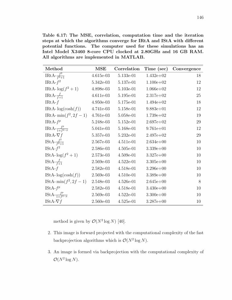
146
Table 6.17: The MSE, correlation, computation time and the iterationsteps at which the algorithms converge for IRtA and IStA with differentpotential functions. The computer used for these simulations has anIntel Model X3460 8-core CPU clocked at 2.80GHz and 16 GB RAM.All algorithms are implemented in MATLAB.
Method MSE Correlation Time (sec) Convergence
IRtA- f2
f2+14.615e-03 5.133e-01 1.432e+02 18
IRtA-f 2 5.342e-03 5.137e-01 1.100e+02 12
IRtA- log(f 2 + 1) 4.898e-03 5.103e-01 1.066e+02 12
IRtA- ff+1
4.611e-03 5.195e-01 2.317e+02 25
IRtA-f 4.950e-03 5.175e-01 1.494e+02 18
IRtA- log(cosh(f)) 4.741e-03 5.158e-01 9.883e+01 12
IRtA- min(f 2, 2f − 1) 4.761e-03 5.058e-01 1.739e+02 19
IRtA-fp 5.248e-03 5.152e-01 2.697e+02 29
IRtA- fp
1+f2−p 5.041e-03 5.168e-01 9.761e+01 12
IRtA-∇f 5.357e-03 5.232e-01 2.497e+02 29
IStA- f2
f2+12.567e-03 4.511e-01 2.634e+00 10
IStA-f 2 2.586e-03 4.505e-01 3.339e+00 10
IStA- log(f 2 + 1) 2.573e-03 4.509e-01 3.327e+00 10
IStA- ff+1
2.569e-03 4.522e-01 3.305e+00 10
IStA-f 2.582e-03 4.518e-01 3.296e+00 10
IStA- log(cosh(f)) 2.569e-03 4.510e-01 3.389e+00 10
IStA- min(f 2, 2f − 1) 2.548e-03 4.526e-01 2.645e+00 8
IStA-fp 2.582e-03 4.518e-01 3.430e+00 10
IStA- fp
1+f2−p 2.569e-03 4.522e-01 3.300e+00 10
IStA-∇f 2.560e-03 4.525e-01 3.287e+00 10
method is given by O(N2 logN) [40].
2. This image is forward projected with the computational complexity of the fast
backprojection algorithms which is O(N2 logN).
3. An image is formed via backprojection with the computational complexity of
O(N2 logN).

147
Assuming that there are k iterations, the computational complexity of IStA is given
by O(kN2 logN). Since k N the computational complexity of the overall method
is given by O(N2 logN).
In comparison, the edge-preserving algebraic reconstruction method described
in [50] has a computational complexity of O(N4). The linear programming and
the OMP based techniques described in [88] have the computational complexities of
O(N7/2), O(N3), respectively. Finally, the subspace pursuits technique presented in
[88] has the computational complexity between O(N2 logN) and O(N3) depending
on the sparsity of the measurements.
6.8 Conclusion
In this chapter, we describe novel, computationally efficient algorithms for
SAR image reconstruction suitable for the limited (or sparse) aperture SAR data
corrupted by noise. First, an iterative reweighted-type algorithm is described in
which Lp-norm constrained SAR image reconstruction problem is approximated with
L2-norm constrained inversion problems iteratively. At every iteration, the solution
obtained in the previous iteration is used to determine the filter of the new FBP
operator. To increase the sharpness of the reconstructed target scene, we use the
edge enhancement filter described in the previous chapter. Then, we introduce an
iterative shrinkage-type algorithm which includes repeated applications of forward
projection and backprojection operators. We demonstrate the performances of the
proposed methods with both synthetic data and the CV dome data set for different
scenerios. Finally, we compare the performances of the new methods with those of
other sparse signal recovery methods.

CHAPTER 7
CONCLUSION
Measurement noise is ubiquitous in SAR data and targets are often embedded in
clutter. There are analytical and numerical optimization-based techniques to ad-
dress these challenges. Analytic techniques are widely used because of their com-
putationally efficiency. However, they do not address noise and clutter explicitly.
There are also numerical optimization-based techniques. These methods use dis-
crete statistical or deterministic models. However, these methods are known to
be computationally intensive. In this thesis, we develop computationally efficient
analytical solutions for SAR image formation in the presence of noise and clutter.
First, we describe a statistical SAR inversion method to suppress noise and
clutter. We present, a novel class of non-stationary stochastic processes to rep-
resent radar targets and clutter. We refer to this class of non-stationary pro-
cesses as pseudo-stationary. They can be considered as locally stationary processes
driven by the Wiener process. We develop analytic filtered-backprojection- and
backprojection-filtering-type methods based on the minimum mean square error
criterion for SAR image reconstruction when the target and clutter scenes belong to
this class of non-stationary processes. The optimal filter that suppresses noise and
clutter depends on the space-varying spectral densities of the target and clutter. We
describe a method to estimate these quantities directly from the SAR data during
the image reconstruction process.
We investigate the performance of this method theoretically. We apply these
methods to both synthetic data and the real SAR data. Next, we develop an analytic
inversion formula based on a best linear unbiased estimation criterion when the
clutter is a pseudo-stationary process. We assume that the target is deterministic
and demonstrate the performance of the method with numerical simulations.
We investigate non-quadratic prior models to represent target scenes in the
second part of the thesis. Specifically, we consider edge preserving prior models
that is also applicable to SAR imaging with limited data or sparse aperture. We
148

149
formulate the image reconstruction as non-quadratic optimization problems and
describe two methods for SAR inversion. First, we present an iterative reweighted-
type algorithm. The optimization problem is approximated with a sequence of L2-
norm constrained problems and solved iteratively with a sequence of FBP operators.
At every iteration, we use the solution obtained in the previous step to determine
the filter of the FBP operator. The second method is a shrinkage-type method.
The algorithm is gradient-based and consists of iterative applications of forward
projection and backprojection operators.
We also present a novel edge enhancement method that is applicable directly
to the SAR received signal. The method enhances the edges in desired directions
in the reconstructed image. This novel filter simultaneously reconstructs SAR im-
ages and enhances edges of the objects in the reconstructed image. We use this
method to sharpen the reconstructed images for IRtA and IStA. We demonstrate
the performances of the edge enhancement and the sparse recovery methods both
with the synthetic data and the CV dome data set. We also compare the compu-
tational complexities and the computation times of these algorithms with those of
other state-of-the-art sparse signal recovery techniques.
Noise/clutter suppression techniques are essential for SAR imaging. Moreover,
it is also desirable to reconstruct SAR images with limited data and sparse aperture.
One of the biggest challenges for real-time SAR imaging is the immense computation
power required to form images and the necessity of real-time operation in many
applications. Therefore, it becomes a necessity to develop computationally efficient,
fast-backprojection algorithms and to use parallel programming techniques.
While we develop IRtA and IStA with noise as the only disturbance term, we
can easily extend these methods to include clutter. Additionally, the optimal filter
designed for the non-stationary target and clutter, and edge enhancement methods
can be modified further for object classification purposes in automatic target recog-
nition applications. Another topic to look into for the methods developed in this
thesis may be developing algorithms that do not require additional data to estimate
clutter space-varying spectral density functions.
Finally, all the methods described in this thesis can be easily applied to other

150
imaging modalities such as X-Ray computed tomography, sonar and geophysical
imaging in which forward operator is modeled as FIOs.

BIBLIOGRAPHY
[1] C. E. Yarman et al., “Bistatic synthetic aperture radar imaging for arbitrary
flight trajectories,” IEEE Trans. Image Process., vol. 17, no. 1, pp. 84–93,
Jan. 2008.
[2] K. E. Dungan et al., “Wide angle SAR data for target discrimination
research,” in Proc. SPIE, Algorithms for SAR Imagery XIX, vol. 8394, May
2012, p. 83940M.
[3] C. J. Nolan and M. Cheney, “Synthetic aperture inversion for arbitrary flight
paths and nonflat topography,” IEEE Trans. Image Process., vol. 12, no. 9,
pp. 1035–1043, Sept. 2003.
[4] V. Krishnan et al., “Multistatic synthetic aperture radar image formation,”
IEEE Trans. Image Process., vol. 19, no. 5, pp. 1290–1306, May 2010.
[5] S. Hensley et al., “The UAVSAR instrument: Description and first results,”
in Proc. IEEE Radar Conf., 2008, pp. 1–6.
[6] T. Yue-sheng et al., “A multi-mode UAV SAR real-time signal processor
system,” in Proc. IEEE 2nd Asian-Pacific SAR Conf., 2009, pp. 947–950.
[7] H. Essen et al., “SUMATRA, a W-band SAR for UAV application,” in Proc.
IEEE Int. Radar Conf., 2009, pp. 1–4.
[8] W. Wang et al., “Waveform-diversity-based millimeter-wave UAV SAR
remote sensing,” IEEE Trans. Geosci. Remote Sens., vol. 47, no. 3, pp.
691–700, Mar. 2009.
[9] M. Edwards et al., “MicroASAR: A small, robust LFM-CW SAR for
operation on UAVs and small aircraft,” in Proc. IEEE Int. Geosci. Remote
Sens. Symp., vol. 5, 2008, pp. V–514.
151

152
[10] J. Muoz et al., “INTA’s developments for UAS and small platforms:
QUASAR,” in Proc. IEEE Int. Geosci. Remote Sens. Symp., vol. 4, 2009,
pp. IV–999.
[11] E. Peterson et al., “A feasibility assessment for low-cost InSAR
formation-flying microsatellites,” IEEE Trans. Geosci. Remote Sens., vol. 47,
no. 8, pp. 2847–2858, Aug. 2009.
[12] J. Coker and A. Tewfik, “Performance synthesis of UAV trajectories in
multistatic SAR,” IEEE Trans. Aerosp. Electron. Syst., vol. 47, no. 2, pp.
848–863, Apr. 2011.
[13] P. Zhan et al., “Adaptive mobile sensor positioning for multi-static target
tracking,” IEEE Trans. Aerosp. Electron. Syst., vol. 46, no. 1, pp. 120–132,
Feb. 2010.
[14] J. Coker and A. Tewfik, “Compressed sensing and multistatic SAR,” in Proc.
IEEE Int. Conf. Acoust., Speech, Signal Process., 2009, pp. 1097–1100.
[15] J. Coker, “Signal processing algorithms for simplified-hardware multistatic
synthetic aperture radar,” Ph.D. dissertation, Dept. of Electr. & Comput.
Eng., Univ. Minnesota, Minneapolis, MN, 2008.
[16] C. E. Yarman and B. Yazici, “Synthetic aperture hitchhiker imaging,” IEEE
Trans. Image Process., vol. 17, no. 11, pp. 2156–2173, Nov. 2008.
[17] I. Cumming and J. Bennett, “Digital processing of SEASAT SAR data,” in
Proc. IEEE Int. Conf. Acoust., Speech, Signal Process., vol. 4, 1979, pp.
710–718.
[18] J. C. Curlander and R. N. McDonough, Synthetic Aperture Radar, New
York, NY: John Wiley & Sons, 1991.
[19] R. Raney et al., “Precision SAR processing using chirp scaling,” IEEE
Trans. Geosci. Remote Sens., vol. 32, no. 4, pp. 786–799, July 1994.

153
[20] C. Cafforio et al., “SAR data focusing using seismic migration techniques,”
IEEE Trans. Aerosp. Electron. Syst., vol. 27, no. 2, pp. 194–207, Mar. 1991.
[21] R. Bamler, “A comparison of range-Doppler and wavenumber domain SAR
focusing algorithms,” IEEE Trans. Geosci. Remote Sens., vol. 30, no. 4, pp.
706–713, July 1992.
[22] R. Stolt, “Migration by Fourier transform,” Geophysics, vol. 43, no. 1, pp.
23–48, Feb. 1978.
[23] J. L. Walker, “Range-Doppler imaging of rotating objects,” IEEE Trans.
Aerosp. Electron. Syst., vol. AES–16, no. 1, pp. 23–52, Jan. 1980.
[24] A. W. Doerry. (2012, May). Basics of Polar-Format Algorithm for processing
synthetic aperture radar images. Sandia Nat. Laboratories, Albuquerque,
NM and Livermore, CA. [Online]. Available:
http://prod.sandia.gov/techlib/access-control.cgi/2012/123369.pdf
(Retrieved on July 20, 2014).
[25] B. Yazici et al., “Synthetic-aperture inversion in the presence of noise and
clutter,” Inverse Problems, vol. 22, no. 5, p. 1705, Oct. 2006.
[26] R. Fa et al., “Knowledge-aided STAP algorithm using convex combination of
inverse covariance matrices for heterogenous clutter,” in Proc. IEEE Int.
Conf. Acoust., Speech, Signal Process., 2010, pp. 2742–2745.
[27] J. Roman et al., “Parametric adaptive matched filter for airborne radar
applications,” IEEE Trans. Aerosp. Electron. Syst., vol. 36, no. 2, pp.
677–692, Apr. 2000.
[28] K. Sohn et al., “Parametric GLRT for multichannel adaptive signal
detection,” IEEE Trans. Signal Process., vol. 55, no. 11, pp. 5351–5360, Nov.
2007.
[29] P. Wang et al., “A new parametric GLRT for multichannel adaptive signal
detection,” IEEE Trans. Signal Process., vol. 58, no. 1, pp. 317–325, Jan.
2010.

154
[30] T. Kragh and A. Kharbouch, “Monotonic iterative algorithms for SAR image
restoration,” in Proc. IEEE Int. Conf. Image Process., 2006, pp. 645–648.
[31] C. Bouman and K. Sauer, “A generalized Gaussian image model for
edge-preserving MAP estimation,” IEEE Trans. Image Process., vol. 2, no. 3,
pp. 296–310, Jul. 1993.
[32] R. Bose et al., “Sequence CLEAN: A modified deconvolution technique for
microwave images of contiguous targets,” IEEE Trans. Aerosp. Electron.
Syst., vol. 38, no. 1, pp. 89–97, Jan. 2002.
[33] M. McClure and L. Carin, “Matching pursuits with a wave-based dictionary,”
IEEE Trans. Signal Process., vol. 45, no. 12, pp. 2912–2927, Dec. 1997.
[34] A. Brito et al., “Sar image superresolution via 2-D adaptive extrapolation,”
Multidimensional Syst. and Signal Process., vol. 14, no. 1–3, pp. 83–104, Jan.
2003.
[35] M. Pinheiro and M. Rodriguez-Cassola, “Reconstruction methods of missing
SAR data: analysis in the frame of TanDEM-X synchronization link,” in
Proc. 9th European Conf. SAR, 2012, pp. 742–745.
[36] W. Rao et al., “ISAR imaging of maneuvering targets with missing data via
matching pursuit,” in Proc. IEEE Radar Conf., 2011, pp. 124–128.
[37] Y. Wang et al., “Nonparametric spectral analysis with missing data via the
EM algorithm,” Digit. Signal Process., vol. 15, no. 2, pp. 191–206, Mar. 2005.
[38] Y. Wang et al., “Spectral Analysis of Signals: The Missing Data Case,”
Synthesis Lectures on Signal Process. Series, vol. 1, no. 1, pp. 1–102, Jan.
2006.
[39] S. Nilsson, “Application of fast backprojection techniques for some inverse
problems of integral geometry,” Ph.D. dissertation, Dept. of Mathematics,
Linkoping University, Linkoping, Sweden, 1997.

155
[40] L. M. Ulander et al., “Synthetic-aperture radar processing using fast
factorized back-projection,” IEEE Trans. Aerosp. Electron. Syst., vol. 39,
no. 3, pp. 760–776, July 2003.
[41] M. Priestley, Spectral Analysis and Time Series, London, United Kingdom:
Academic press, 1981.
[42] K. E. Dungan et al., “Civilian vehicle radar data domes,” in Proc. SPIE,
Algorithms for SAR Imagery XVII, vol. 7699, 2010, p. 76990P.
[43] J. Duistermaat, Fourier Integral Operators, vol. 130, New York, NY:
Birkhauser, 1996.
[44] J. Treves, Introduction to Pseudodifferential and Fourier Integral Operators,
vol. 2, New York, NY: Springer, 1980.
[45] A. Grigis and J. Sjostrand, Microlocal Analysis for Differential Operators:
An Introduction, vol. 196, ser. London Mathematical Soc. Lecture Note
Series, New York, NY: Cambridge University Press, 1994.
[46] B. Yazıcı and V. Krishnan. (2010, Mar. 15). Microlocal Analysis in Imaging.
[Online]. Available: http:
//www.ecse.rpi.edu/∼yazici/ICASSPTutorial/microlocal ICASSP10.html
(Retrieved on July 10, 2014).
[47] G. Beylkin, “Imaging of discontinuities in the inverse scattering problem by
inversion of a causal generalized Radon transform,” J. Math. Phys., vol. 26,
no. 1, pp. 99–108, Jan. 1985.
[48] Y. Abramovich et al., “Two-dimensional multivariate parametric models for
radar applications-part II: Maximum-entropy extensions for hermitian-block
matrices,” IEEE Trans. Signal Process., vol. 56, no. 11, pp. 5527–5539, Nov.
2008.
[49] J. Bergin et al., “Improved clutter mitigation performance using
knowledge-aided space-time adaptive processing,” IEEE Trans. Aerosp.
Electron. Syst., vol. 42, no. 3, pp. 997 –1009, July 2006.

156
[50] M. Cetin and W. C. Karl, “Feature-enhanced synthetic aperture radar image
formation based on nonquadratic regularization,” IEEE Trans. Image
Process., vol. 10, no. 4, pp. 623–631, Apr. 2001.
[51] W. Melvin and J. Guerci, “Knowledge-aided signal processing: a new
paradigm for radar and other advanced sensors,” IEEE Trans. Aerosp.
Electron. Syst., vol. 42, no. 3, pp. 983–996, July 2006.
[52] P. Stoica et al., “On using a priori knowledge in space-time adaptive
processing,” IEEE Trans. Signal Process., vol. 56, no. 6, pp. 2598–2602, June
2008.
[53] D. Vu et al., “Nonparametric missing sample spectral analysis and its
applications to interrupted SAR,” IEEE J. Sel. Topics in Signal Process.,
vol. 6, no. 1, pp. 1–14, Feb. 2012.
[54] B. Yazici et al., “Synthetic aperture inversion with sparsity constraints,” in
Proc. IEEE Int. Conf. Electromagn. in Advanced Appl., 2011, pp. 1404–1407.
[55] S. R. DeGraaf, “SAR imaging via modern 2-D spectral estimation methods,”
IEEE Trans. Image Process., vol. 7, no. 5, pp. 729–761, May 1998.
[56] J. Li and P. Stoica, “An adaptive filtering approach to spectral estimation
and SAR imaging,” IEEE Trans. Signal Process., vol. 44, no. 6, pp.
1469–1484, June 1996.
[57] Z. Bi et al., “Super resolution SAR imaging via parametric spectral
estimation methods,” IEEE Trans. Aerosp. Electron. Syst., vol. 35, no. 1, pp.
267–281, Jan. 1999.
[58] E. G. Larsson and J. Li, “Spectral analysis of periodically gapped data,”
IEEE Trans. Aerosp. Electron. Syst., vol. 39, no. 3, pp. 1089–1097, July 2003.
[59] R. Wu et al., “SAR image formation via semiparametric spectral
estimation,” IEEE Trans. Aerosp. Electron. Syst., vol. 35, no. 4, pp.
1318–1333, Oct. 1999.

157
[60] F. Lombardini and A. Reigber, “Adaptive spectral estimation for
multibaseline SAR tomography with airborne L-band data,” in Proc. IEEE
Int. Geosci. Remote Sens. Symp., vol. 3, 2003, pp. III–2014.
[61] S. Xiao and D. C. Munson Jr., “Spotlight-mode SAR imaging of a
three-dimensional scene using spectral estimation techniques,” in Proc. IEEE
Int. Geosci. Remote Sens. Symp., vol. 2, 1998, pp. 642–644.
[62] X. X. Zhu and R. Bamler, “Super-resolution power and robustness of
compressive sensing for spectral estimation with application to spaceborne
tomographic SAR,” IEEE Trans. Geosci. Remote Sens., vol. 50, no. 1, pp.
247–258, Jan. 2012.
[63] Z. Liu et al., “Efficient implementation of Capon and APES for spectral
estimation,” IEEE Trans. Aerosp. Electron. Syst., vol. 34, no. 4, pp.
1314–1319, Oct. 1998.
[64] M. Xue et al., “IAA spectral estimation: fast implementation using the
Gohberg–Semencul factorization,” IEEE Trans. Signal Process., vol. 59,
no. 7, pp. 3251–3261, July 2011.
[65] L. Borcea et al., “Adaptive interferometric imaging in clutter and optimal
illumination,” Inverse Problems, vol. 22, no. 4, p. 1405, Aug. 2006.
[66] J. Garnier and K. Sølna, “Coherent interferometric imaging for synthetic
aperture radar in the presence of noise,” Inverse Problems, vol. 24, no. 5, p.
055001, Oct. 2008.
[67] J. Swoboda et al., “Bistatic synthetic aperture radar imaging for arbitrary
trajectories in the presence of noise and clutter,” in Proc. SPIE, Airborne
Intell., Surveillance, Reconnaissance Syst. and Appl. VI, vol. 7307, 2009, p.
73070D.
[68] K. Voccola et al., “On the relationship between the generalized likelihood
ratio test and backprojection for synthetic aperture radar imaging,” in Proc.
SPIE, Automat. Target Recognition XIX, vol. 7335, 2009, p. 73350I.

158
[69] V. Krishnan and B. Yazici, “Synthetic aperture radar imaging exploiting
multiple scattering,” Inverse Problems, vol. 27, no. 5, p. 055004, May 2011.
[70] K. Voccola et al., “Polarimetric synthetic-aperture inversion for extended
targets in clutter,” Inverse Problems, vol. 29, no. 5, p. 054003, May 2013.
[71] M. Cetin et al., “Sparsity-driven synthetic aperture radar imaging:
Reconstruction, autofocusing, moving targets, and compressed sensing,”
IEEE Signal Process. Mag., vol. 31, no. 4, pp. 27–40, July 2014.
[72] P. Stoica and R. L. Moses, Introduction to Spectral Analysis, vol. 1, Upper
Saddle River, NJ: Prentice Hall, 1997.
[73] R. O. Schmidt, “Multiple emitter location and signal parameter estimation,”
IEEE Trans. Antennas Propag., vol. AP–34, no. 3, pp. 276–280, Mar. 1986.
[74] R. Roy and T. Kailath, “ESPRIT-estimation of signal parameters via
rotational invariance techniques,” IEEE Trans. Acoust., Speech, Signal
Process., vol. 37, no. 7, pp. 984–995, July 1989.
[75] J. Capon, “Maximum-Likelihood Spectral Estimation,” in Nonlinear Methods
of Spectral Analysis, New York, NY: Springer-Verlag, 1983, pp. 155–179.
[76] J. Li and P. Stoica, “Efficient mixed-spectrum estimation with applications
to target feature extraction,” IEEE Trans. Signal Process., vol. 44, no. 2, pp.
281–295, Feb. 1996.
[77] J. Ward, “Space-time adaptive processing for airborne radar,” in Inst. Elect.
Eng. Colloq. STAP, 1998, p. 2.
[78] A. Farina and P. Lombardo, “Space-time techniques for SAR,” in Appl.
Space-Time Adaptive Process., London, United Kingdom: Inst. Elect. Eng.,
2004, pp. 73–122.
[79] D. Cerutti-Maori et al., “Experimental verification of SAR-GMTI
improvement through antenna switching,” IEEE Trans. Geosci. Remote
Sens., vol. 48, no. 4, pp. 2066–2075, Apr. 2010.

159
[80] W. L. Melvin, “A STAP overview,” IEEE Trans. Aerosp. Electron. Syst.,
vol. 19, no. 1, pp. 19–35, Jan. 2004.
[81] E. Wigner, “On the quantum correction for thermodynamic equilibrium,”
Physical Rev., vol. 40, no. 5, p. 749, June 1932.
[82] V. Krishnan and E. Quinto, “Microlocal aspects of common offset synthetic
aperture radar imaging,” Inverse Problems and Imag., vol. 5, no. 3, pp.
659–674, Aug. 2011.
[83] M. Priestley, “Evolutionary spectra and non-stationary processes,” J. Roy.
Statistical Soc. Series B (Methodological), vol. 27, no. 2, pp. 204–237, 1965.
[84] E. Candes et al., “Fast computation of Fourier integral operators,” SIAM J.
Sci. Comput., vol. 29, no. 6, pp. 2464–2493, Oct. 2007.
[85] E. J. Kelly, “An adaptive detection algorithm,” IEEE Trans. Aerosp.
Electron. Syst., vol. AES–2, no. 2, pp. 115–127, Mar. 1986.
[86] T. Yardibi et al., “Source localization and sensing: A nonparametric iterative
adaptive approach based on weighted least squares,” IEEE Trans. Aerosp.
Electron. Syst., vol. 46, no. 1, pp. 425–443, Jan. 2010.
[87] X. Tan et al., “Sparse learning via iterative minimization with application to
MIMO radar imaging,” IEEE Trans. Signal Process., vol. 59, no. 3, pp.
1088–1101, Mar. 2011.
[88] W. Dai and O. Milenkovic, “Subspace pursuit for compressive sensing signal
reconstruction,” IEEE Trans. Inf. Theory, vol. 55, no. 5, pp. 2230–2249, May
2009.
[89] D. Shnidman, “Generalized radar clutter model,” IEEE Trans. Aerosp.
Electron. Syst., vol. 35, no. 3, pp. 857–865, July 1999.
[90] R. Gonzalez and R. Woods, Digital Image Processing, 3rd ed. Upper Saddle
River, NJ: Prentice-Hall, Inc., 2008.

160
[91] C. J. Nolan and M. Cheney, “Synthetic aperture inversion,” Inverse
Problems, vol. 18, no. 1, p. 221, Feb. 2002.
[92] J. Canny, “A computational approach to edge detection,” IEEE Trans.
Pattern Anal. Mach. Intell., vol. PAMI–8, no. 6, pp. 679–698, Nov. 1986.
[93] J. Bruder and R. Schneible, “Interrupted SAR waveforms for high interrupt
ratios,” in Proc. IET Int. Conf. Radar Syst., 2007, pp. 1–5.
[94] J. Salzman et al., “Interrupted synthetic aperture radar (SAR),” IEEE
Trans. Aerosp. Electron. Syst. Mag., vol. 17, no. 5, pp. 33–39, May 2002.
[95] M. Ferrara et al., “Resolution optimization with irregularly sampled Fourier
data,” Inverse Problems, vol. 29, no. 5, p. 054007, May 2013.
[96] J. N. Ash, “Joint imaging and change detection for robust exploitation in
interrupted SAR environments,” in Proc. SPIE, Algorithms for SAR
Imagery XX, vol. 8746, 2013, p. 87460J.
[97] I. Stojanovic et al., “Reconstruction of interrupted SAR imagery for
persistent surveillance change detection,” in Proc. SPIE, Algorithms for SAR
Imagery XIX, vol. 8394, 2012, p. 839408.
[98] L. C. Potter et al., “Sparsity and compressed sensing in radar imaging,”
Proc. IEEE, vol. 98, no. 6, pp. 1006–1020, June 2010.
[99] J. H. Ender, “On compressive sensing applied to radar,” Signal Process.,
vol. 90, no. 5, pp. 1402–1414, May 2010.
[100] M. A. Herman and T. Strohmer, “High-resolution radar via compressed
sensing,” IEEE Trans. Signal Process., vol. 57, no. 6, pp. 2275–2284, June
2009.
[101] R. Baraniuk and P. Steeghs, “Compressive radar imaging,” in Proc. IEEE
Radar Conf., 2007, pp. 128–133.
[102] M. Herman and T. Strohmer, “Compressed sensing radar,” in Proc. IEEE
Radar Conf., 2008, pp. 1–6.

161
[103] E. J. Candes et al., “Stable signal recovery from incomplete and inaccurate
measurements,” Commun. Pure and Appl. Mathematics, vol. 59, no. 8, pp.
1207–1223, Aug. 2006.
[104] D. L. Donoho, “Compressed sensing,” IEEE Trans. Inf. Theory, vol. 52,
no. 4, pp. 1289–1306, Apr. 2006.
[105] S. Mallat and Z. Zhang, “Matching pursuits with time-frequency
dictionaries,” IEEE Trans. Signal Process., vol. 41, no. 12, pp. 3397–3415,
Dec. 1993.
[106] J. Burns et al., “Adaptive decomposition in electromagnetics,” in Proc.
IEEE Antennas and Propag. Soc. Int. Symp., vol. 3, 1997, pp. 1984–1987.
[107] P. S. Huggins and S. W. Zucker, “Greedy basis pursuit,” IEEE Trans. Signal
Process., vol. 55, no. 7, pp. 3760–3772, July 2007.
[108] D. Needell and J. A. Tropp, “CoSaMP: Iterative signal recovery from
incomplete and inaccurate samples,” Appl. and Comput. Harmonic Anal.,
vol. 26, no. 3, pp. 301–321, May 2009.
[109] J. A. Tropp, “Greed is good: Algorithmic results for sparse approximation,”
IEEE Trans. Inf. Theory, vol. 50, no. 10, pp. 2231–2242, Oct. 2004.
[110] J. A. Tropp et al., “Algorithms for simultaneous sparse approximation. Part
I: Greedy pursuit,” Signal Process., vol. 86, no. 3, pp. 572–588, Mar. 2006.
[111] S. S. Chen et al., “Atomic decomposition by basis pursuit,” SIAM J. Sci.
Comput., vol. 20, no. 1, pp. 33–61, Aug. 1998.
[112] S. Chen and D. Donoho, “Basis pursuit,” in Rec. 28th Asilomar Signals,
Syst. and Computers Conf., vol. 1, 1994, pp. 41–44.
[113] I. Daubechies et al., “Iteratively reweighted least squares minimization for
sparse recovery,” Commun. Pure and Appl. Mathematics, vol. 63, no. 1, pp.
1–38, Jan. 2009.

162
[114] B. D. Rao and K. Kreutz-Delgado, “An affine scaling methodology for best
basis selection,” IEEE Trans. Signal Process., vol. 47, no. 1, pp. 187–200,
Jan. 1999.
[115] E. J. Candes et al., “Enhancing sparsity by reweighted l-1 minimization,” J.
Fourier Anal. and Appl., vol. 14, no. 5-6, pp. 877–905, Dec. 2008.
[116] D. L. Donoho and J. M. Johnstone, “Ideal spatial adaptation by wavelet
shrinkage,” Biometrika, vol. 81, no. 3, pp. 425–455, Sept. 1994.
[117] D. L. Donoho et al., “Wavelet shrinkage: asymptopia?” J. Roy. Statistical
Soc. Series B (Methodological), vol. 57, no. 2, pp. 301–369, 1995.
[118] D. L. Donoho and I. M. Johnstone, “Minimax estimation via wavelet
shrinkage,” The Ann. Statist., vol. 26, no. 3, pp. 879–921, June 1998.
[119] M. A. Figueiredo et al., “Majorization–minimization algorithms for
wavelet-based image restoration,” IEEE Trans. Image Process., vol. 16,
no. 12, pp. 2980–2991, Dec. 2007.
[120] I. Daubechies et al., “An iterative thresholding algorithm for linear inverse
problems with a sparsity constraint,” Commun. Pure and Appl.
Mathematics, vol. 57, no. 11, pp. 1413–1457, Nov. 2004.
[121] M. A. Figueiredo and R. D. Nowak, “An EM algorithm for wavelet-based
image restoration,” IEEE Trans. Image Process., vol. 12, no. 8, pp. 906–916,
Aug. 2003.
[122] M. A. Figueiredo and R. D. Nowak, “A bound optimization approach to
wavelet-based image deconvolution,” in Proc. IEEE Int. Conf. Image
Process., vol. 2, 2005, pp. II–782.
[123] T. Blumensath and M. E. Davies, “Iterative thresholding for sparse
approximations,” J. Fourier Anal. and Appl., vol. 14, no. 5-6, pp. 629–654,
Dec. 2008.

163
[124] H. Guo et al., “Speckle reduction via wavelet shrinkage with application to
synthetic-aperture-radar-based automatic target detection/reduction
(ATD/R),” in Proc. SPIE, Wavelet Appl. in Signal and Image Process. II,
vol. 2303, 1994, pp. 333–344.
[125] A. Achim et al., “SAR image denoising via Bayesian wavelet shrinkage based
on heavy-tailed modeling,” IEEE Trans. Geosci. Remote Sens., vol. 41,
no. 8, pp. 1773–1784, Aug. 2003.
[126] A. Beck and M. Teboulle, “A fast iterative shrinkage-thresholding algorithm
for linear inverse problems,” SIAM J. Imag. Sciences, vol. 2, no. 1, pp.
183–202, Mar. 2009.
[127] A. Pizurica et al., “Despeckling SAR images using wavelets and a new class
of adaptive shrinkage estimators,” in Proc. IEEE Int. Conf. Image Process.,
vol. 2, 2001, pp. 233–236.
[128] D. Wei et al., “Simultaneous speckle reduction and data compression using
best wavelet packet bases with application to synthetic aperture radar
(SAR) based ATD/R,” in Proc. SPIE, Wavelet Appl. II, vol. 2941, 1995, pp.
1131–1141.
[129] G. Davis et al., “Adaptive greedy approximations,” Constructive
Approximation, vol. 13, no. 1, pp. 57–98, 1997.
[130] M. Elad, Sparse and Redundant Representations: From Theory to
Applications in Signal and Image Processing, New York, NY:
Springer-Verlag, 2010.
[131] C. Bouman and K. Sauer, “A generalized Gaussian image model for
edge-preserving MAP estimation,” IEEE Trans. Image Process., vol. 2, no. 3,
pp. 296–310, July 1993.
[132] C. A. Bouman et al., (1995, Oct. 23-26). Markov Random Fields and
Stochastic Image Models. [Online]. Available: http://www.cis.temple.edu/

164
∼latecki/Courses/RobotFall08/Papers/MRFBauman.pdf (Retrieved on
October 23, 2014).
[133] R. Chellappa and A. Jain, Markov Random Fields: Theory and Application,
vol. 1, Boston, MA: Academic Press, 1993.
[134] J. Besag, “Spatial interaction and the statistical analysis of lattice systems,”
J. Roy. Statistical Soc. Series B (Methodological), vol. 36, no. 2, pp. 192–236,
1974.
[135] R. Kindermann et al., Markov Random Fields and Their Applications, vol. 1,
Providence, RI: Amer. Math. Soc., 1980.
[136] A. Blake, “Comparison of the efficiency of deterministic and stochastic
algorithms for visual reconstruction,” IEEE Trans. Pattern Anal. Mach.
Intell., vol. 11, no. 1, pp. 2–12, Jan. 1989.
[137] J. Besag, “Towards Bayesian image analysis,” J. Appl. Stat., vol. 20, no. 5-6,
pp. 107–119, 1993.
[138] R. Stevenson and E. Delp, “Fitting curves with discontinuities,” in Proc. 1st
Int. Workshop on Robust Comput. Vision, 1990, pp. 127–136.
[139] P. J. Green, “Bayesian reconstructions from emission tomography data using
a modified EM algorithm,” IEEE Trans. Med. Imag., vol. 9, no. 1, pp. 84–93,
Mar. 1990.
[140] S. Ganan and D. McClure, “Bayesian image analysis: an application to single
photon emission tomography,” in Proc. Statistical Comput. Section, 1985,
pp. 12–18.
[141] J.-B. Thibault et al., “A three-dimensional statistical approach to improved
image quality for multislice helical CT,” Med. Physics, vol. 34, no. 11, pp.
4526–4544, Nov. 2007.

165
[142] D. Geman and G. Reynolds, “Constrained restoration and the recovery of
discontinuities,” IEEE Trans. Pattern Anal. Mach. Intell., vol. 14, no. 3, pp.
367–383, Mar. 1992.
[143] T. Hebert and R. Leahy, “A generalized EM algorithm for 3-d bayesian
reconstruction from Poisson data using Gibbs priors,” IEEE Trans. Med.
Imag., vol. 8, no. 2, pp. 194–202, June 1989.
[144] I. F. Gorodnitsky and B. D. Rao, “Sparse signal reconstruction from limited
data using FOCUSS: A re-weighted minimum norm algorithm,” IEEE Trans.
Signal Process., vol. 45, no. 3, pp. 600–616, Mar. 1997.
[145] H. C. Yanik et al., “Computationally efficient FBP-type direct segmentation
of synthetic aperture radar images,” in Proc. SPIE, Algorithms for SAR
Imagery XVIII, vol. 8051, 2011, p. 80510C.
[146] K. Pearson, “Mathematical contributions to the theory of evolution.–on a
form of spurious correlation which may arise when indices are used in the
measurement of organs,” Proc. Roy. Soc. London, vol. 60, no. 359–367, pp.
489–498, Jan. 1896.
[147] T. Hastie et al., The Elements of Statistical Learning, vol. 2, no. 1, New
York, NY: Springer, 2009.
[148] B. Efron et al., “Least angle regression,” The Ann. Statist., vol. 32, no. 2,
pp. 407–499, Apr. 2004.
[149] R. Tibshirani, “Regression shrinkage and selection via the LASSO,” J. Roy.
Statistical Soc. Series B (Methodological), vol. 58, no. 1, pp. 267–288, 1996.
[150] M. D. Plumbley, “On polar polytopes and the recovery of sparse
representations,” IEEE Trans. Inf. Theory, vol. 53, no. 9, pp. 3188–3195,
Sept. 2007.
[151] D. L. Donoho et al., “Sparse solution of underdetermined systems of linear
equations by stagewise orthogonal matching pursuit,” IEEE Trans. Inf.
Theory, vol. 58, no. 2, pp. 1094–1121, Feb. 2012.

166
[152] Stanford University. (2007, May 26). SparseLAB. [Online]. Available:
http://sparselab.stanford.edu/ (Retrieved on July 20, 2014).
[153] Y. S. Abu-Mostafa et al., Learning from Data, AMLBook.com, 2012.
[154] S. M. Kay, Fundamentals of Statistical Processing, vol. 1, Upper Saddle
River, NJ: Prentice Hall, 1993.
[155] D. L. Donoho and M. Elad, “Optimally sparse representation in general
(nonorthogonal) dictionaries via L1 minimization,” Proc. Nat. Academy
Sciences, vol. 100, no. 5, pp. 2197–2202, Mar. 2003.
[156] E. J. Candes et al., “Robust uncertainty principles: Exact signal
reconstruction from highly incomplete frequency information,” IEEE Trans.
Inf. Theory, vol. 52, no. 2, pp. 489–509, Feb. 2006.
[157] E. J. Candes and T. Tao, “Decoding by linear programming,” IEEE Trans.
Inf. Theory, vol. 51, no. 12, pp. 4203–4215, Dec. 2005.

APPENDIX A
METHOD OF THE STATIONARY PHASE
Let u be a smooth function of compact support in Rn and let φ be a real-valued
function with only non-degenerate critical points. A point x0 ∈ Rn is called a
non-degenerate critical point if ∇φ(x0) = 0 where
∇φ(x0) =
∇x1φ
∇x2φ
. (A.1)
and the Hessian matrix of φ has non-zero determinant. The stationary phase theo-
rem states that as λ→∞∫eiλφ(x)u(x)dnx =
(2π
λ
)n/2 ∑x0:∇φ(x0)=0
u(x0)eiλφ(x0)ei(π/4)sgn(Hxφ(x0))√
| detHxφ(x0)|
+O(λ−n/2−1) (A.2)
where Hx(φ(x0)) denotes the Hessian of φ given by:
Hx(φ(x0)) =
∇x21φ ∇x1,x2φ
∇x2,x1φ ∇x22φ
. (A.3)
167

APPENDIX B
PROOF OF THE LEMMA 1
(i) We write
J Tns(Q) =
∫E[|(KnsF − IΩ)[T ](z)|2] dz. (B.1)
By using (3.33),
J Tns(Qns) =
∫ei2π[(x−z)·ξ−(x′−z)·ξ′][Qns(z, ξ)A(x, ξ)η(x, z, ξ)− χΩ(z, ξ)]
× [Qns(z, ξ′)A(x′, ξ′)η(x′, z, ξ′)− χΩ(z, ξ′)]
×RT (x,x′)dξdxdx′dξ′dz,
(B.2)
where χΩ(z, ξ) is a function that prevents division by 0. We apply the method
of the stationary phase in the variables z, ξ′ for the phase
φ4(x, z, ξ,x′, ξ′) = (x− z) · ξ − (x′ − z) · ξ′ (B.3)
We check the Hessian:
Hz,ξ′(φ4) =
∇z2φ4 ∇z,ξ′φ4
∇ξ′,zφ4 ∇ξ′2φ4
=
. (B.4)
det(Hz,ξ′(φ4)) = −1 where =
0 0
0 0
and =
0 1
1 0
. Therefore, we get
the critical points
∇zφ4 → ξ′ = ξ, (B.5)
∇ξ′φ4 → z = x′. (B.6)
168

169
The leading-order term of B.2 can be written as
J Tns(Qns) ≈
∫ei2π(x−x′)·ξ[Qns(x
′, ξ)A(x, ξ)η(x,x′, ξ)− χΩ(x′, ξ)]RT (x,x′)
× [Qns(x′, ξ′)A(x′, ξ′)η(x′,x′, ξ′)− χΩ(x′, ξ′)] dξdxdx′.
(B.7)
Writing
RT (x,x′) =
∫ei2π(x−x′)·ζST (x, ζ)ST (x′, ζ) dζ (B.8)
we obtain
J Tns(Qns) ≈
∫ei2π[(x−x′)·ξ+(x−x′)·ζ][Qns(x
′, ξ)A(x, ξ)η(x,x′, ξ)− χΩ(x′, ξ)]
× [Qns(x′, ξ′)A(x′, ξ′)η(x′,x′, ξ′)− χΩ(x′, ξ′)]
× ST (x, ζ)ST (x′, ζ)dxdx′dξdζ.
(B.9)
We apply the method of the stationary phase one more time in the variables
x′, ζ for the phase
φ5(x, ξ,x′, ζ) = (x− x′) · ξ + (x− x′) · ζ (B.10)
We check the Hessian:
Hx′,ζ(φ5) =
∇x′2φ5 ∇x′,ζφ5
∇ζ,x′φ5 ∇ζ2φ5
=
. (B.11)
detHz,ξ′(φ5) = −1, therefore we get the critical points at
∇x′φ5 → ζ = ξ, (B.12)
∇ζφ5 → x′ = x. (B.13)

170
The leading order term of (B.9) is then
J Tns(Qns) ≈
∫ ∣∣Qns(x, ξ)A(x, ξ)η(x,x, ξ)− χΩ(x, ξ)∣∣2|ST (x, ξ)|2dξdx.
(B.14)
To obtain an approximation to J Cns(Qns), we follow the same steps (B.1)-(B.14)
and get
J Cns(Qns) ≈
∫ ∣∣Qns(x, ξ)A(x, ξ)η(x,x, ξ)∣∣2|SC(x, ξ)|2dξdx. (B.15)
For J nns(Qns), we first write
J nns(Qns) :=
∫E[Kns[n](z)Kns[n](z′)] dz
=
∫ei2πω(t−R(s,z)/c)Qns(z, s, ω)σ2(s)Rn(t, t′)
× e−i2πω′(t′−R(s,z′)/c)Qns(z′, s, ω)dωdω′dtdsdt′dzdz′ (B.16)
Inserting (3.17) into (B.16) and carrying out the integrations over t, t′, ω′,
gives
J nns(Qns) =
∫ei2πω(R(s,z′)−R(s,z))/cQns(z, s, ω)Qns(z′, s, ω)
× |Sn(s, ω)|2dωdsdzdz′. (B.17)
In (B.17), we apply the same change of variables as in (3.28). This transforms
(B.17) to
J nns(Qns) ≈
∫ei2π(z′−z)·ξQns(z, ξ)Qns(x′, ξ)η(z, z, ξ)|Sn(ξ)|2dξdzdz′.
(B.18)
By following a similar argument in [25], if the noise power spectral density
decays slowly for large ξ, then Jn(Q) has singularities at x′ = x and we

171
obtain
J nns(Qns) ≈
∫|Qns(z, ξ)||Sn(ξ)|2η(z, z, ξ)dξdz. (B.19)
(ii) Using the approximation obtained in (3.39) for KbpF and following the steps in
(B.1)-(B.14), the leading-order singularities of J Tbp(Qbp), J C
bp (Qbp) and J nbp(Qbp)
are given by (B.14), (B.15) and (B.19) with Qns replaced by Qbp where Qbp is
defined by (3.43)
Qbp(z,x′) =
∫ei2π(x′−z)·ξ′Qbp(z, ξ
′)dξ′. (B.20)

APPENDIX C
PROOF OF THE THEOREM 1
(i) We have
Jns(Q′) = J Tns(Q
′) + J Cns(Q
′) + J nns(Q
′). (C.1)
Let us fix a function Qε and for some small ε consider a variation of the form
Q′ = Qns+ εQε. This is substituted into (3.24) - (3.26) and differentiated with
respect to ε and then ε is set to 0. This results in
0 =d
dεJ Tns(Qns + εQε)
∣∣∣∣ε=0
+d
dεJ Cns(Qns + εQε)
∣∣∣∣ε=0
+d
dεJ nns(Qns + εQε)
∣∣∣∣ε=0
.
(C.2)
From (3.40), the first term on the right side of (C.2) is
d
dεJ Tns(Qns + εQε)
∣∣∣∣ε=0
≈∫QεAη|ST |2(QnsAη − χ) dξdx
+
∫(QnsAη − χ)|ST |2QεAη dξdx (C.3)
which can be written as
d
dεJ Tns(Qns + εQε)
∣∣∣∣ε=0
≈ 2Re
∫QεAη|ST |2(QnsAη − χ) dξdx. (C.4)
Similarly,
d
dεJ Cns(Qns + εQε)
∣∣∣∣ε=0
≈ 2Re
∫QεAη|SC |2QnsAη dξdx (C.5)
and
d
dεJ nns(Qns + εQε)
∣∣∣∣ε=0
≈ 2Re
∫|Sn|2QεQnsη dξdz. (C.6)
172

173
Recall that
Jns(Qns) = J Tns(Qns) + J C
ns(Qns) + J nns(Qns). (C.7)
Thus, using (C.4), (C.5) and (C.6),
d
dεJ (Qns + εQε)
∣∣∣∣ε=0
≈2Re
∫Qε
(∫Aη(QnsAη(|ST |2 + |SC |2)− |ST |2χ
)+
× |Sn|2Qnsη
)dξdx.
(C.8)
In order for the right hand side of (C.8) to be 0 for all Qε,the second integrand
inside the parenthesis needs to be zero.∫Aη(QnsAη(|ST |2 + |SC |2)− |ST |2χ
)+ |Sn|2Qnsη dξdx = 0 (C.9)
which reduces to
Aη(QnsAη − χΩ)|ST |2 + AηQnsAη|SC |2 +Qnsη|Sn|2 = 0. (C.10)
From (C.10) the filter Qns can be explicitly written as follows:
Qns(z, ξ) = Q1ns(z, ξ)Q2
ns(z, ξ) (C.11)
where
Q1ns(z, ξ) =
A(z, ξ)χΩ
|A(z, ξ)|2η(z, z, ξ), (C.12)
Q2ns(z, ξ) =
|ST (z, ξ)|2
|ST (z, ξ)|2 + |SC(z, ξ)|2 + |Sn(ξ)|2|A(z,ξ)|2η(z,z,ξ)
(C.13)
where Q1ns is the same filter derived in [1]. Ωz is the data collection manifold
given by (3.34) |ST (z, ξ)|2 and |SC(z, ξ)|2 are the SVSD functions defined in
(3.11) and (3.13). |Sn(ξ)|2 is the noise power spectral density function defined
in (3.17).

174
(ii) Using the approximation obtained in (3.39) for KbpF and following the steps
in (C.1)-(C.10), the leading-order singularities of the filter Qbp that minimizes
the (leading-order) MSE Jbp(Qbp) is given by
Qbp(z,x′) =
∫ei2π(z−x′)·ζQns(z, ζ)dζ. (C.14)
(iii) We calculate the MSE between the true and the reconstructed target scenes
with filter given in (3.44) as follows
J (Qns) =JT (Qns) + JC(Qns) + Jn(Qns) (C.15)
≈∫ ∣∣Qns(x, ξ)A(x, ξ)η(x,x, ξ)− χΩ(x, ξ)
∣∣2|ST (x, ξ)|2dξdx
+
∫ ∣∣Qns(x, ξ)A(x, ξ)η(x,x, ξ)|2|SC(x, ξ)|2dξdx
+
∫|Qns(z, ξ)|2|Sn(ξ)|2η(z, z, ξ)dξdz. (C.16)
Inserting Qns = Q1nsQ
2ns into (C.16), we write
Jns(Qns) ≈∫ ∣∣Q2
ns(x, ξ)− χΩ(x, ξ)∣∣2|ST (x, ξ)|2dξdx
+
∫ ∣∣Q2ns(x, ξ)|2|SC(x, ξ)|2dξdx
+
∫|Q2
ns(z, ξ)|2 |Sn(ξ)|2
|A(x, ξ)|2η(z, z, ξ)dξdz. (C.17)
We expand the first term in (C.17) and write
Jns(Qns) ≈∫ |Q2
ns(x, ξ)|2(|ST (x, ξ)|2 + |SC(x, ξ)|2 +
|Sn(ξ)|2
|A(x, ξ)|2η(z, z, ξ)
)+(|χΩ(x, ξ)
∣∣2 − 2Q2ns(x, ξ)χΩ(x, ξ)
)|ST (x, ξ)|2
dξdx.
(C.18)
Inserting (C.13) into (C.18), we obtain
J (Qns) = J (Q1nsQ
2ns) =
∫α(x, ξ)|ST (x, ξ)|2
|ST (x, ξ)|2 + α(x, ξ)χΩ(x, ξ)dξdx (C.19)

175
where
α(x, ξ) = |SC(x, ξ)|2 +|Sn(ξ)|2
|A(x, ξ)|2η(x,x, ξ). (C.20)
We can obtain the MSE for BPF method by replacing Qns with Qbp which
results in the same MSE up to the leading-order.
We investigate the statistics of the reconstructed images in detail in Appendix D.

APPENDIX D
STATISTICS OF THE RECONSTRUCTED IMAGES
In this section, we investigate the deviation of the reconstructed target scene from
the true scene and calculate a compensation term. In Appendix C it was shown
that
J (Qns) = J (Q1nsQ
2ns) =
∫α(x, ξ)|ST (x, ξ)|2
|ST (x, ξ)|2 + α(x, ξ)χΩ(x, ξ)dξdx, (D.1)
and inserting only Q1ns into J (Qns)
J 1ns(Q
1ns) =
∫α(x, ξ)χΩ(x, ξ)dξdx. (D.2)
are the MSE between true and the reconstructed target scenes with (C.12) and
(C.13), respectively where
α(x, ξ) = |SC(x, ξ)|2 +|Sn(ξ)|2
|A(x, ξ)|2η(x,x, ξ). (D.3)
We assume that the Fourier transform of the windowing function Φ is 1. It should
be noted here that Tns(z) is an MMSE for T (x) and (C.19) is the variance of this
estimator.
Equations (C.19) and (D.2) show that an increase in clutter or noise level
results in a greater error for filter Q1ns compared to Qns.
It is important to note that these error terms are valid with the assumption
that the full knowledge of the target and clutter SVSD functions are available. How-
ever, as it is mentioned in earlier chapters, we form an image of the target/clutter
scenes to estimate the target and the clutter SVSD functions. Therefore, the vari-
ance of the MMSE for the non-stationary reconstruction method described in Chap-
176

177
ter 3 is:
Jns(Q1ns, Q
2ns) =
∫E[|Tns(z)− T (z)|2
]dz (D.4)
=
∫E[|KnsF [T1 + C1](z) +Kns[n](z)− T (z)|2
]dz (D.5)
=
∫E[|KnsF [T1](z)− T (z)|2 + |KnsF [C1](z)|2 + |Kns[n](z)|2
− 2ReKF(KF)†[T1C1] − 2ReKnsFK†ns[T1n]
− 2ReKnsFK†ns[C1n]]dz
(D.6)
where T1(z) = K1F [T +C] +K1[n] and C1(z) = K1F [C] +K1[n] and K1 is the FBP
operator with filter Q1ns. Now we write∫
E[|KnsF [T1](z)− T (z)|2
]dz =
∫E[KnsFT1T1F †K†ns
− 2ReKnsF [T1T ]+ T T]dz. (D.7)
For the first term of (D.7) we write:∫E[KnsFT1T1F †K†ns
]dz =
∫|QnsQ1|Aη|2|2(|ST |2 + |SC |2 + |Sn|2/|A|2η)dξdz
(D.8)
For the second term of (D.7) we have,∫E[ReKnsF [T1T ]
]dz
=
∫E[ReKnsFK1F [T T ] +KnsFK1F [CT ] +KnsFK1[nT ]
]dξdz (D.9)
=
∫ReQnsQ1|Aη|2|ST |2dξdz (D.10)
since the target is uncorrelated with noise and clutter. For the fourth term of (D.4)

178
we write∫E[ReKnsF(KnsF)†[T1C1]
]dz =
∫|QnsQ1|2|Aη|4(|SC |2 + |Sn|2/|A|2η)dξdz,
(D.11)
for the fifth term of (D.4)∫E[ReKnsFK†ns[T1n]
]dz =
∫Re|Qns|2Q1η|Aη|2|Sn|2dξdz (D.12)
and for the sixth term of (D.4) we have∫E[ReKnsFK†ns[C1n]
]dz =
∫Re|Qns|2Q1η|Aη|2|Sn|2dξdz. (D.13)
Similarly, we write∫E[|KnsF [C1](z)|2
]dz =
∫E[|KnsFK1F [C] +KnsFK1[n]|2
]dz (D.14)
=
∫|QnsQ1|2|Aη|4(|SC |2 + |Sn|2/|A|2η)dξdz (D.15)
and finally we write∫E[|Kns[n](z)|2
]dz ≈
∫|Qns|2|Sn|2ηdξdz. (D.16)
Thus, Jns is given by
Jns(Q1ns, Q
2ns) ≈
∫|QnsQ1|Aη|2|2(|ST |2 + |SC |2 + |Sn|2/|A|2η)dξdz
− 2
∫ReQnsQ1|Aη|2|ST |2dξdz +
∫|ST |2dξdz
+
∫|QnsQ1|Aη|2|2(|SC |2 + |Sn|2/η)dξdz +
∫|Q|2|Sn|2ηdξdz
− 2
∫Re|QnsQ1|Aη|2|2(|SC |2 + |Sn|2/|A|2η)dξdz
− 4
∫Re|Qns|2Q1η|Aη|2|Sn|2dξdz. (D.17)

179
Therefore, we have
Jns(Qns) ≈∫ |ST (x, ξ)|2(|α(x, ξ)|2 − 3 |ST (x,ξ)Sn(ξ)|2
|A(x,ξ)|2η(x,x,ξ))
(|ST (x, ξ)|2 + α(x, ξ))2dξdx (D.18)
where Tns(z) is the image of the target scene reconstructed by (C.13) by using the
SVSD functions formed by (C.12).
Integrand inside (D.18) can be considered as the SVSD function of the error
term due to not using the true target and clutter SVSD functions, i.e.
Tns(z) = T (z) + εns(z) → |STns(ξ)|2 = |ST (ξ)|2 + |Sεns(ξ)|2. (D.19)
The error given in (C.19) can be reduced by compensating for the estimated target
SVSD function with |Sεns(ξ)|2. Thus, the best possible image that can be recon-
structed after compensating for the error has the variance∫α(x, ξ)|ST (x, ξ)|4
|ST (x, ξ)|4 + α(x,ξ)(|ST (x,ξ)|2+α(x,ξ))2
|ST (x,ξ)|2+2α(x,ξ)+3|Sn(ξ)|2
|A(x,ξ)|2η(x,x,ξ)
χΩ(x, ξ)dξdx (D.20)
where α is given by (D.3), χΩ is a smooth function that prevents division by 0,
|Sn|2 is the noise spectral density function, and |ST |2, |SC |2, are SVSD functions for
target and clutter, respectively.

APPENDIX E
ESTIMATION OF THE SVSD FUNCTIONS
In this section, we briefly describe a method introduced in [41], [83] for the spec-
tral density function estimation of non-stationary processes. The method can be
viewed as a straightforward extension of the spectral density function estimation for
stationary processes.
Theorem 3: Let Φ(x) be a square integrable, compactly supported windowing
function satisfying the conditions in [83, eq. (7.5), eq. (7.6)] and f(x) denote a real-
ization of a zero-mean pseudo-stationary process with the SVSD function |Sf (x, ξ)|2.
Let βf and βφ denote the maximum intervals over which f and Φ can be considered
as stationary, respectively [83, eq. (7.3)]. We define:
Uξ0(x) =
∫ΩΦ
Φ(u)f(x− u)e−iξ0·(x−u)du (E.1)
where
βφ βf ΩΦ (E.2)
and u ∈ R2, ΩΦ is the support of the windowing function and ξ0 is any constant
frequency. We assume that for each pixel x0, the neighborhood of f(x0), x0 ∈ ΩΦ
is stationary, i.e. f(x) is locally stationary for each x. Then, U(x) represents the
Fourier transform of every locally stationary neighborhood of f(x). Following [41]
we write ∫RUξ0
(x,x+ τ)ei2πζ·τdτ ≈ |Φ(ζ)|2|Sf (x, ζ)|2, (E.3)
i.e. Fourier transform of RUξ0(x,x + τ) = E
[Uξ0
(x)Uξ0(x+ τ)
]is an estimator
for the space-varying spectral density function of f(x) where Φ(ξ) is the Fourier
transform of Φ(x) normalized to 1.
Proof: To prove (E.3), we adapt the estimation method for semi-stationary pro-
180

181
cesses presented in [41] into our model. Let f(x) denote a zero-mean pseudo-
stationary process. f(x) can be expressed in the mean square sense as
f(x) =
∫ei2π(x−x′)·ξSf (x, ξ) dξdB(x′). (E.4)
Using (3.8), (3.48) can be written as
Uξ0(x) =
∫Φ(u)e−i2π(x−x′−u)·ξ0ei2π(x−x′−u)·ξSf (x− u, ξ)e−i2πx′·ξ0dudξdB(x′).
(E.5)
Next, Ψx,λ(θ) is defined such that
Ψx,λ(θ) =
∫Φ(u)
Sf (x− u, λ)
Sf (x, λ)e−i2πθ·udu. (E.6)
We rearrange the terms in (E.5)
Uξ0(x) =
∫Φ(u)
Sf (x− u, ξ)
Sf (x, ξ)e−i2π(ξ−ξ0)·uei2π(ξ−ξ0)·u
× Sf (x, ξ)ei2π(x−x′−u)·(ξ−ξ0)e−i2πx′·ξ0dudξdB(x′). (E.7)
We make the change of variables ξ = ξ + ξ0 and use the definition (E.6)
Uξ0(x) =
∫Ψx,ξ+ξ0
(ξ)Sf (x, ξ + ξ0)ei2π(x−x′)·ξe−i2πx′·ξ0dξdB(x′). (E.8)
Next, we calculate RUξ0(x,x′) = E[Uξ0
(x)Uξ0(x′)] as follows:
RUξ0(x,x′) =E[Uξ0
(x)Uξ0(x′)]
=
∫Ψx,ξ+ξ0
(ξ)Sf (x, ξ + ξ0)ei2π(x−x′′)·ξe−i2πx′′·ξ0Ψx′,ξ′+ξ0(ξ)
× Sf (x′, ξ′ + ξ0)e−i2π(x′−x′′′)·ξ′ei2πx′′′·ξ0E[dB(x′′)dB(x′′′)]dξdξ′.
(E.9)

182
Using E[dB(x′)dB(x′′)] = δ(x′′ − x′′′)dx′′′dx′′, (E.9) can be written as
RUξ0(x,x′) =
∫Ψx,ξ+ξ0
(ξ)Sf (x, ξ + ξ0)ei2π(x−x′′)·ξe−i2πx′′·ξ0Ψx′,ξ′+ξ0(ξ)
× Sf (x′, ξ′ + ξ0)e−i2π(x′−x′′′)·ξ′ei2πx′′′·ξ0δ(x′′ − x′′′)dx′′dx′′′dξdξ′
(E.10)
=
∫Ψx,ξ+ξ0
(ξ)Sf (x, ξ + ξ0)ei2π(x·ξ−x′·ξ′)Ψx′,ξ′+ξ0(ξ)Sf (x′, ξ
′ + ξ0)
× ei2π(ξ−ξ′)·x′′dx′′dξdξ′
(E.11)
∫ei2π(ξ−ξ′)·x′′dx′′dξ′ = δ(ξ − ξ′)dξ′, thus
RUξ0(x,x′) =
∫Ψx,ξ+ξ0
(ξ)Ψx′,ξ+ξ0(ξ)Sf (x, ξ + ξ0)Sf (x′, ξ + ξ0)ei2π(x−x′)·ξdξ
(E.12)
Now we let x′ = x+ τ and calculate the Fourier transform∫RUξ0
(x,x+ τ)ei2πζ·τdτ =
∫Ψx,ξ+ξ0
(ξ)Ψx+τ,ξ+ξ0(ξ)ei2πτ ·(ζ−ξ)
× Sf (x, ξ + ξ0)Sf (x+ τ, ξ + ξ0)dξdτ. (E.13)
By using Ψx,ξ+ξ0(ξ)Ψx+τ,ξ+ξ0
(ξ) ≈ |Φ(ξ)|2 and following a similar argument in [25],
we assume that Sf (x, ξ + ξ0) decays slowly for large ξ. Then, the integration in
(E.13) has singularities at ξ = ζ and we write∫RUξ0
(x,x+ τ)ei2πζ·τdτ ≈ |Φ(ζ)|2|Sf (x, ζ + ξ0)|2, (E.14)
i.e. Fourier transform of RUξ0(x,x) is an (approximately) unbiased estimator for
space-varying spectral density function of the target for frequencies around ξ0 for
each pixel x.

APPENDIX F
A SHORT REVIEW ON BLUE
Let x = [x[0], x[1], . . . , x[N − 1]] denote a dataset corresponding to measurements
of the original signal s = [s[0], s[1], . . . , s[N − 1]] given by
x[n] = θs[n] + w[n] (F.1)
where w is the disturbance term.
Let p(x; θ) denote the probability distribution function (PDF) of this random
variable depending on an unknown variable θ. Finally, let θ denote an estimator for
the parameter θ.
Bias and variance of an estimator generally gives a good idea whether an
estimator is a good one or not. The bias and the variance of the estimator θ are
defined as follows:
BIAS(θ) :=E[θ]− θ, (F.2)
VAR(θ) :=E[‖θ − E[θ]‖2
2
]. (F.3)
The mean-square-error (MSE) is a widely-used figure of merit to determine the
performance of an estimator and it is defined as
MSE(θ) := E[‖θ − θ‖2
2
]. (F.4)
MSE can be expanded as
MSE(θ) =E[‖θ − θ‖2
2
](F.5)
=‖BIAS(θ)‖22 + VAR(θ) (F.6)
which shows the well-known trade-off between the bias and the variance of an esti-
mator. (F.6) shows that having a zero-bias, zero-variance estimator is not possible
183

184
almost always. Therefore, one needs to design the estimator by considering the
fact that if the estimator has zero-bias it will have large variance and vice verse.
From a machine learning point of view, (F.6) can be interpreted as the fact that a
training dataset can be underfit (low variance, large bias) or overfit (low bias, large
variance) [153].
Having low-bias results in more generalizable estimators. Moreover, often
times only the bias depends on the unknown parameters. Therefore, it is usually
more desirable to design estimators that has zero bias and the minimum variance.
This is also equivalent to finding an unbiased estimator that minimizes the MSE
among all other estimators.
An estimator θ is said to be a minimum variance unbiased estimator (MVUE)
if [154]
• E[θ] = θ, ∀θ ∈ Θ,
• If E[˜θ] = θ, ∀θ ∈ Θ, then VAR(θ) ≤ VAR(
˜θ), ∀θ ∈ Θ.
where Θ is the set that includes all the estimators θ. As specified in the definition
of MVUE, one needs to look through all possible estimators to find the minimum
variance estimator. Therefore, it may not be possible to find the MVUE as PDF or
the model may not be known completely. As a solution to this problem, a suboptimal
estimator may be restricted to be a linear one. Then the linear estimator, that has
the minimum variance is called the best linear unbiased estimator (BLUE).
As stated earlier there are three conditions for an estimator to be BLUE. For
measurements x:
1. Estimator needs to be linear:
θ =N−1∑n=0
anx[n]. (F.7)
provided that∑N−1
n=0 an = 1

185
2. Bias needs to be 0:
E[θ] =N−1∑n=0
anE[x[n]] = θ. (F.8)
3. Estimator must be a solution to the problem
minθ
VAR(θ) = minθ
E
(N−1∑n=0
anx[n]− E
[N−1∑n=0
anx[n]
])2 . (F.9)
Using a = [a0, a1, . . . , aN−1]T , (F.9) can be written as
VAR(θ) =E[(aTx− aTE[x])2] (F.10)
=E[aT (x− aTE[x])(x− aTE[x])Ta] (F.11)
=aTCa (F.12)
where C = E[(x − aTE[x])(x − aTE[x])T ]. Therefore, the problem given in (F.9)
becomes identical to finding a that minimizes aTCa. To minimize variance of the
estimator aTCa subject to the constraint aT s we use Lagrange multipliers
J(a, λ) = aTCa− λ(aT s− 1). (F.13)
We calculate the derivative with respect to a and set it equal to zero:
∂
∂aJ(a, λ) = 0 = 2Ca∗ + λs→ a∗ = λ
C−1s
2(F.14)
where a∗ is a vector containing the optimal weights for the estimator. Using the
constraint equation
aT s = 1→ λsTC−1
2s = 1 (F.15)

186
and λ is given by
λ =2
sTC−1s. (F.16)
Therefore, the BLUE is given by [154]
θ =sTC−1x
sTC−1s(F.17)
with the minimum variance
VAR(θ) =1
sTC−1s(F.18)
and the bias
E[θ] =sTC−1E[x]
sTC−1s=
sTC−1s
sTC−1s= θ. (F.19)
Let θ = q2q1x, then we have
q1 = sTC−1 (F.20)
q2 =1
sTC−1s=λ
2. (F.21)
With vector parameters, if the data model is given by
x = Hθ + w (F.22)
then the BLUE is
θ =(HTC−1H
)−1HTC−1x (F.23)
with the minimum variance
Cθ =(HTC−1H
)−1(F.24)
where C is the covariance matrix of the noise. This is also known as the Gauss-

187
Markov Theorem [154] and if w is Gaussian then BLUE is MVUE.
Similar to the scalar case, if we let θ = Q2Q1x
Q1 = HTC−1 (F.25)
Q2 =(HTC−1H
)−1. (F.26)
If MVUE is linear then BLUE given in (F.17) is indeed the MVUE and it only
requires the first and second order statistics of the given data.

APPENDIX G
CALCULATION OF THE HESSIANS FOR CHAPTER 4
G.1 Hessian Matrix for (4.38)
Hessian for the phase function
φ1(x,x′, z, ζ, ξ) = (x′ − z) · ζ + (x− x′) · ξ (G.1)
is evaluated as follows
Hx′,ζ(φ1) =
∇2x′2φ1 ∇2
x′,ζφ1
∇2ζ,x′φ1 ∇2
ζ2φ1
=
(G.2)
det(Hx′,ζ(φ1)) = −1 where =
0 0
0 0
and =
0 1
1 0
.
G.2 Hessian Matrix for (4.48)
Hessian for the phase function
φ2(x, ξ, x, ξ, z) = (x− z) · ξ − (x− z) · ξ (G.3)
is evaluated as follows
Hz,ξ(φ2) =
∇2z2φ2 ∇2
z,ξφ2
∇2ξ,zφ2 ∇2
ξ2φ2
=
(G.4)
and det(Hz,ξ(φ2)) = −1.
188

189
G.3 Hessian Matrix for (4.53)
Hessian for the phase function
φ3(x, x, ξ, ζ) = (x− x) · ξ − (x− x) · ζ (G.5)
is evaluated as follows
Hx,ζ(φ3) =
∇2x2φ3 ∇2
x,ζφ3
∇2ζ,xφ3 ∇2
ζ2φ3
=
(G.6)
and det(Hx,ζ(φ3)) = −1.

APPENDIX H
CONDITIONS FOR THE SPARSE SIGNAL RECOVERY
Under some conditions, we can replace L0-norm with Lp-norm and define
min |T|1 subject to |d− FT|22 ≤ ε (H.1)
where p is set to 1. (6.3) is a convex relaxation of (6.2) [109]. In order to guarantee
the sparsest solution with S nonzero entries, F must satisfy the following conditions:
1. The mutual coherence of F defined by µ(F) = maxi 6=j |hHi hj| should satisfy
|T|0 ≤1
2(1 + µ−1(F)) (H.2)
where the superscript H denotes the Hermitian and hi is the ith column of
F [155].
2. The restricted isometric constant (RIC) of F, [156], [157] denoted by δS ∈(0, 1), must satisfy for every submatrix FS composed from any S columns of
F
(1− δs)|T|22 ≤ |FST|22 ≤ (1 + δS)|T|22 (H.3)
where the RIC and the mutual coherence are related by [155]–[157]
δS ≤ (S − 1)µ(F). (H.4)
190